An improved Probabilistic Seismic Hazard Assessment of Tripura, India

Abstract

The State of Tripura lies in northeast India which is considered to be one of the most seismically active regions of the world. In the present study, a realistic Probabilistic Seismic Hazard Assessment (PSHA) of Tripura State based on improved seismogenic sources considering layered polygonal sources corresponding to hypo-central depth range of $0-25$ km, $25-70$ km and $70-180$ km, respectively and data driven selection of suitable Ground Motion Prediction Equations (GMPEs) in a logic tree framework is presented. Analyses have been carried out by formulating a layered seismogenic source zonation together with smooth-gridded seismicity. Using the limited accelerogram records available, most suitable GMPEs have been selected after performing a thorough quantitative assessment and thus the uncertainty in selecting appropriate GMPEs in PSHA has been addressed by combining them with proper weight factor. The computations of seismic hazard are carried out in a higher resolution of grid interval of 0.05$\degree$ $\times$ 0.05$\degree$. The probabilistic seismic hazard distribution in terms of Peak Ground Acceleration (PGA) and $5\%$ damped Pseudo Spectral Acceleration (PSA) at different time periods for $10\%$ and $2\%$ probability of exceedance in $50$ years at engineering bedrock level have been presented. The final results show significant improvements over the previous studies, which is reflecetd in the local variation of the hazard maps. The design response spectra at engineering bedrock level can be computed for any location in the study region from the hazard distributions. The results will be useful for earthquake resistant design and construction of structures in this region.

1 Introduction

Hazards associated with earthquakes are commonly referred to as seismic hazards and ground shaking is considered to be the most important of all seismic hazards because all the other hazards are consequences of ground shaking (Kramer, 2013). Ground shaking causes extensive damage to properties and lives in a seismic prone terrain possessing favourable seismo-tectonics and local geological site conditions. It thus necessitates to estimate seismic hazard of the terrain under consideration in a realistic way, which could provide the necessary design inputs for earthquake resistant design of structures.

Northeast India is one of the most highly seismic active regions which record more than seven earthquakes of magnitudes 5 and above per year on an average (Sitharam and Sil, 2014). The State of Tripura is one of the eight northeastern states of India and from the seismological point of view, Tripura is considered to be of interest due to the existence of the important geotectonic unit Tripura Fold Belt to the west of Indo-Burmese ranges. Compressive movements between the Indian plate and the Eurasian plate during Oligocene to recent times produced the Tripura Fold Belt (Gupta, 2006). Besides that, Tripura is surrounded by Eastern Himalaya and the Shillong Plateau-Mikir Hills in the north, the Naga-Disang Thrust system in the northeast, the Tertiary fold-thrust belt of the Indo-Burma Arc in the east and the Bengal Basin in the southwest.

In the region surrounded by Tripura, 18 events of magnitude $M_{w}>7.0$ have taken place since 1664 (shown in Figure 1) and the impacts of these earthquakes have attracted the attention of scientists and engineers towards seismic safety evaluation of the region. The latest seismic zoning map of India released by Bureau of Indian Standards (BIS) assigns four levels of seismicity in terms of zone factor (BIS, 1893-2016), which is twice the zero period acceleration (ZPA) of the design spectrum. The present study area falls in seismic zone $V$ with the highest zone factor $0.36$ as per BIS (1893-2016). However, the crucial limitation of the seismic zonation code of India (BIS, 1893-2016) is that it is not based on comprehensive seismic hazard analysis and hence it lacks the probabilistic features (Khattri, 2006). However, the probabilistic approach in the computation of seismic hazard analysis is considered to be more appropriate and realistic for its scientifically sound background Kramer (2013). PSHA approach has the property that with a specified confidence level, the ground motion will not be exceeded at any of the time periods due to any of the earthquakes expected during a given time interval, thus taking the randomness of the earthquake occurrences in space, time and magnitude into account. The computational formulation of probabilistic seismic hazard assessment (PSHA) was developed by Cornell (1968); McGuire (1976).

Basu and Nigam (1977) and Khattri et al. (1984) adopted a probabilistic approach to prepare seismic zonation maps in terms of peak ground acceleration (PGA) for a specific return period. Bhatia et al. (1999) performed a probabilistic seismic hazard assessment (PSHA) of India under the Global Seismic Hazard Assessment Program (GSHAP). Many researchers have also carried out the seismic hazard studies of northeastern states of India in the past (Sharma and Malik, 2006; Nath, 2006; Thingbaijam et al., 2008; Raghukanth et al., 2008; Sitharam and Sil, 2014; Das et al., 2016). The present study attempts to improve upon the existing studies to some extent by considering layered polygonal sources corresponding to different hypo-central depths together with smooth-gridded seismicity and data driven selection of ground motion prediction equations (GMPEs). Similar type of methodology has been adopted previously by Nath and Thingbaijam (2012); Maiti et al. (2017). However, the computation of seismic hazard in the present study is carried out in a higher resolution of finer grid interval of $0.05\degree\times 0.05\degree$ and the suitability of different GMPEs against recorded strong motion data of different focal depths are judged by the histograms of normalized residuals and the likelihood values, introduced by Scherbaum et al. (2004).

National Earthquake Hazard Reduction Program (NEHRP) gave a site classification scheme based on the average shear wave velocity for upper 30 m soil column ($V_{S30}$). The standard engineering bedrock or the firm-rock site conditions are considered to be more realistic for the regional hazard computations (Nath and Thingbaijam, 2012) and the standard engineering bedrock corresponds to $V_{S30}$ $\sim$ $760$ m/s (defined as the boundary site class BC). In the present study, the spatial distribution of probabilistic seismic hazard in terms of Peak Ground Acceleration (PGA) and $5\%$ damped Pseudo Spectral Acceleration (PSA) at different time periods for $10\%$ and $2\%$ probability of exceedance in $50$ years (corresponding to return periods $475$ and $2475$ years, respectively) at engineering bedrock have been obtained. The final hazard maps thus produced are able to capture the spatial variations in seismic hazard of Tripura. We expect that the results will be useful to structural engineers for earthquake resistant design of structures and helpful to government for taking decisions regarding disaster mitigation.

2 Region of Study and Seismo-tectonic Framework

The present study is focused on the seismic hazard assessment of Tripura, one of the eight northeastern states in India. The region of study is extended by $300$ km in radius from the geographical boundary of the state of Tripura, $i.e$, a buffer of $300$ km is considered from the geographical boundary of Tripura. Therefore, the region of study ranges from $20\degree$ N - $28\degree$ N in latitude and $88\degree$ E - $96\degree$ E in longitude. The region of study with the important geo-tectonic units is shown in Figure 1. The hill shaded terrain representation SRTM data, used in Figure 1, has been taken from Consortium for Spatial Information (Jarvis et al., 2008).

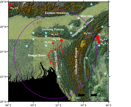
Figure 1: Region of the present study with the important geotectonic units. The solid line in red colour shows the geographical boundary (approximate) of Tripura and the solid line in purple colour shows a buffer of $300$ km. The events in asterix symbol indicate the earthquakes of magnitude $M_{W}>7.0$. The events in filled circle are the strong-motion earthquakes considered for selection of suitable GMPEs.

Northeast India is one of the most seismically active regions of the world (Kayal, 1991). The seismotectonics of northeast India is summarized as south-directed over-thrusting from the north due to collision tectonics at the Himalayan Arc, and northwest directed over-thrusting from the southeast due to subduction tectonics at the Burmese Arc (Mukhopadhyay and Dasgupta, 1988). The study area covers Sheet numbers 13, 14, 16, 24, 25 and 26 of the Seismotectonic Atlas of India and Its Environs (SEISAT) published by Geological Survey India (GSI) (Dasgupta et al., 2000). It is represented by six major tectonic domains namely, the Himalayan mobile belt (Eastern Himalaya) and the Shillong Plateau-Mikir Hills in the north, the Naga-Disang Thrust system in the northeast, the Tertiary fold-thrust belt of the Indo-Burma Arc in the east, the outer molasse basin of Tripura-Chittagong in the south and the Bengal Basin in the southeast. The tectonic features (faults, thrusts, major lineaments etc.) obtained from the SEISAT (Dasgupta et al., 2000), across the study region is depicted in Figure 2.

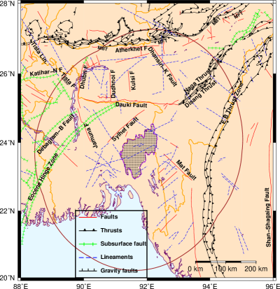
Figure 2: Tectonic map of the study region. The international boundaries, coastlines and water bodies are produced from the Generic Mapping Tools (GMT) database.

The Himalayan mobile belt is represented by four tectonic units in the form of the crystalline complexes (F)F; the folded cover sequences (F)FC; the cover sequences (F)C of Buxa, Miri and Gondwana Groups; and the frontal belt (F) represented by Siwalik Group. These are separated by widespread thrust faults namely, Main Central Thrust (MCT), Main Boundary Thrust (MBT) and Main Frontal Thrust (MFT) and their subsidiary thrusts (Dasgupta et al., 2000). It is a pile of EW oriented thrust faults made of crystalline rocks of the great Himalaya. These thrust faults have overrided the Indian Plate due to the northward underthrusting of Indian Plate beneath southern Tibet (Gansser, 1964). There is N-S convergence within the eastern Himalaya which is accommodated through thrust faulting on shallow north dipping fault plane within the eastern Himalayan wedge (Kumar et al., 2015). The MCT separates two geologically distinct zones — the Lesser Himalaya to the south and the Higher Himalayan Crystallines to the north. The main discontinuity between the sub-Himalayan and lesser Himalaya zones is the MBT, presently marked by intense seismicity and disastrous earthquakes (Angelier and Baruah, 2009).

The Shillong Plateau consist mostly of Archaean Gneissic complex with Proterozoic intracratonic quartzite and phyllite of Shillong group intruded by acid and basic igneous rocks. During the Jurassic-Cretaceous period, the plateau rifted along the southern margin by the E-W steep north dipping Dauki Fault and earthquakes occur to depths of 30-50 km beneath the Shillong plateau (Bilham and England, 2001). Shillong Plateau is characterized by a number of faults, shears and lineaments, which exhibit considerable seismicity. The great 1897 Shillong earthquake ($M_{W}$ 8.0) occurred in the Shillong Plateau which is noted as the largest magnitude earthquake observed in the study area. The north dipping Dauki Fault zone was considered responsible for the same (Oldham, 1899). The N-S striking Dudhnoi and Kulsi faults, the NE striking Barapani and Kalyani shear zones, and several NE-SW and N-S striking lineaments are the other major faults which contribute to the high seismic activity in the Shillong Plateau. In the N-E of Shillong Plateau lies Mikkir hill which is detached from Shillong plateau by seismically active NW-SE striking Kopili-North Dhansiri fault. The Shillong Plateau and Mikir Hills are identified as detached parts of the Indian Plate in the eastern Himalayan syntaxis (Gansser, 1964). In the north, Shillong plateau is limited by Brahmaputra basin, which is characterized by several sets of neotectonic faults of which the NE-SW trending and E-W trending sets are the most conspicuous (Dasgupta et al., 2000).

The Naga-Disang thrust system forms a complex pattern with a narrow belt of imbricate thrust slices, known as the Belt of Schuppen. It is delineated from southeast of Brahmaputra foredeep by Naga thrust on the west and Haflong-Disang thrusts on the east. A number of NNW and NW trending lineaments cut across this over-thrust belt and traverse further south into the Paleogene inner fold belt (Dasgupta et al., 2000). The frontal thrust, although called the Naga thrust, is composed of many different thrusts. The uppermost thrust, known as Disang thrust, overrides all the lower thrusts in the north Cachar Hills. The Disang thrust passes westwards into Dauki fault.

The Indo-Burmese Arc is a very important tectonic feature, and the important structural elements in this part of the region are the high angle reverse faults parallel to the regional north-south folds in the eastern part of the outer arc ridge within the Eastern Boundary Thrust Zone (EBTZ) and the north westerly trending transverse Mat fault (Dasgupta et al., 2000). The Burmese Arc seismicity is an outcome of eastward under thrusting of the Indian Lithosphere below the Burma plate. Santo (1969) illustrates that an inclined seismic zone, defining the Benioff zone, is present throughout Burma. The dip of the Benioff zone was found to $45\degree$ and the depth of penetration about 180km. Seismotectonic studies of the Indo-Burma region have been attempted by several investigators. An eastward dipping zone of seismicity, consistent with the Benioff zone in a typical subduction zone, has been inferred by (Guzman-Speziale and Ni, 1996) who studied the focal mechanisms, focal depth distributions and geometry of Wadati-Benioff zone in this region and suggested that there are no interplate earthquake in this region.

The Tripura-Chittagong fold system is a typical fold-and-thrust belt with west-verging thrusts as a result of the eastward subduction of the Indian Plate (Angelier and Baruah, 2009). It constitutes a different tectonic domain of the Upper Tertiary Surma Basin belonging to the periphery of the Indo-Burma orogen. It comprises of Tripura-Mizoram Hills, The Cittagong hill tracts and Coastal Burma, represents a large Neogene basin formed west of Paleogene Arakan-Yoma Fold Belt and is broadly confined within the Naga Thrust and Dauki Fault to the north and Sylhet Fault and to the west and northwest. The Tripura-Chittagong fold system is composed of narrow, long and doubly plunging folds. The N-S trending folds indicate eastward drag along Dauki Fault in the north. The seismicity in this zone is sparse and the events are mostly shallow focused (Dasgupta et al., 2000).

The Bengal Basin is bordered on its west by the Precambrian basement complex of crystalline metamorphis of the Indian Sheid and to the east by the Tripura- Chittagong Fold Belt. The Bengal Basin comprises of enormous volume of sediments flown down by the Ganga-Brahmaputra drainage system building the world’s largest submarine fan, the Bengal fan. The Bengal fan conceals the northern extension of the Ninety Eastern Ridge and the bathymetric trench, related to subduction of Indian plate (Dasgupta et al., 2000).

Figure 3 shows the seismicity map where the epicenters of the main shocks corresponding to different ranges of hypo-central depths are superimposed on the tectonic map to correlate the past seismicity with the identified tectonic features.

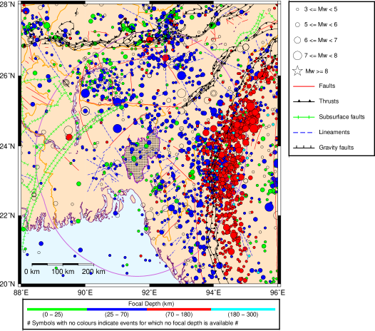
Figure 3: Seismo-tectonic map of the study region depicting the epicenters of the main shocks on the tectonic features.

3 Methodology and Computational Framework

3.1 Preparation of Earthquake Catalogue

The region of the present study ranges from latitude $20\degree$ N - $28\degree$ N and longitude $88\degree$ E - $96\degree$ E. The first step of seismic hazard assessment is to prepare an earthquake catalogue. Earthquake database which contains details of each earthquake event such as time of occurrence in terms of year, month, day, hour and minute; location of occurrence in terms of local magnitude $M_{L}$, surface wave magnitude $M_{S}$, body wave magnitude $m_{b}$ and moment magnitude $M_{W}$ is known as earthquake catalogue. The earthquake catalogue for the present analysis has been prepared from the reviewed International Seismological Centre (ISC) bulletin, UK (http://www.isc.ac.uk/iscbulletin/search/bulletin/), National Earthquake Information Centre (NEIC), (https://earthquake.usgs.gov/earthquakes/search/), USGS and Global Centroid Moment Tensor (GCMT) project supported by the National Science Foundation (https://www.globalcmt.org/CMTsearch.html) for instrumental period and for pre-instrumental and early instrumental period, the database has been taken from various published sources (Jaiswal and Sinha, 2004; Ambraseys, 2000; Oldham, 1869), supplemented with data from India Meteorological Department (IMD), New Delhi. The catalogue compiled for the present study contains a total of $4491$ events starting from 825 A.D. The compiled catalogue contains magnitude in different scales ($M_{L}$, $M_{S}$, $m_{b}$ and $M_{W}$). Conversion of different magnitude scales into one type of magnitude ($M_{W}$) using suitable conversion relations is required to be done for seismic hazard analysis because most of the GMPEs are developed in terms of $M_{W}$ to avoid saturation effects. The process of conversion is termed as homogenization. The homogenization has been carried out using global empirical relations (Filiz and Kartal, 2012; Scordilis, 2006; Sipkin, 2003). The preference or the priority of the type of magnitude taken for homogenization is $M_{W}$ $\rightarrow$ $M_{S}$ $\rightarrow$ $m_{b}$ $\rightarrow$ $M_{L}$. Various conversion relations used in the present study is given in Table 1.

Table 1: Conversion relations used in the present study

Type of
Magnitude	Magnitude range(s)	Conversion relation(s)	Reference(s)
	$3.0$ $\leq$ $M_{S}$ $<$ $6.2$	$M_{W}=0.67M_{S}+2.07$	Scordilis (2006)
$M_{S}$	$6.2$ $\leq$ $M_{S}$ $\leq$ $8.2$	$M_{W}=0.99M_{S}+0.08$	Scordilis (2006)
	$M_{S}$ $>$ $8.2$	$M_{W}=0.8126M_{S}+1.1723$	(Filiz and Kartal, 2012)
	$3.5$ $\leq$ $m_{b}$ $\leq$ 5.5	$M_{W}=0.85m_{b}+1.03$	Scordilis (2006)
$m_{b}$	$5.5$ $<$ $m_{b}$ $\leq$ $7.3$	$M_{W}=1.46m_{b}-2.42$	Sipkin (2003)
	$m_{b}$ $>$ $7.3$	$M_{W}=1.0319m_{b}+0.0223$	(Filiz and Kartal, 2012)
	$M_{L}$ $\leq$ $6.0$	$M_{W}=M_{L}$	Heaton et al. (1986)
$M_{L}$	$M_{L}$ $>$ $6.0$	$M_{W}=0.08095M_{L}+1.30003$	(Filiz and Kartal, 2012)

The seismic events in the catalogue contain main shocks and triggered events (foreshocks and aftershocks). Main shocks are statistically independent and follow Poissonian distribution. Triggered events are dependent on main shocks and tend to cluster in space and time. Seismic hazard analysis is generally based on the assumptions of Poissonian distribution of earthquakes. Therefore it is necessary to identify and remove the foreshocks and the aftershocks from the catalogue. The process to eliminate the dependent events from the earthquake catalogue is known as declustering. The Gardner and Knopoff (1974) window method for identification of dependent events is widely used in practical seismic hazard analysis and the same is adopted here. This approach states that aftershocks are dependent (a non-Poissonian process) on the size of the main shocks and the dependent events need to be removed in accordance with defined distance and time windows. The time window $T(M)$ in days and distance window $L(M)$ in km after Gardner and Knopoff (1974) are as follows:

$$L(M)=10^{0.3238M+0.983}$$

$$T(M)=\begin{cases}10^{0.032M+2.7389}&\text{if $M$ $\geq$ $6.5$}\\ 10^{0.032M+2.7389}&\text{if $M$ $<$ $6.5$}\end{cases}$$ (1)

For any earthquake of magnitude $M$ in the catalogue, the subsequent shocks are identified as aftershock if they occur within the time window $T(M)$ and the distance window $L(M)$. It is more practical to put an upper limit on the magnitude of aftershocks, say at least one unit magnitude below the magnitude of the main shock (Bath, 1965). The method can also be applied to identify the foreshocks, if the time of occurrence is before the time of the shock under consideration and it has not been identified as aftershock of an earlier main shock. No upper limit is required to be put on the magnitude of the foreshock, except that it should be lower than that of the main shock. The declustered earthquake catalogue contains a total of $2694$ main shocks in $M_{W}$ unit, $i.e$, declustering eliminates about $40$$\%$ of the events in the catalogue.

3.2 Delineation of Seismogenic Source Zones

Identification of seismogenic sources is one of the most important steps in seismic hazard assessment. Due to plate boundary activity in northern Himalaya, intraplate activity in Shillong Plateau and subduction process in Indo-Burmese range, the seismotectonic setup observed in the study region is very complex as described in Section 1. Source delineation is primarily based on tectonic trends and seismicity of the region.. However, there are not any consistent criteria for defining seismogenic source zone (SSZ) so far. We found the methodology given by (Nath and Thingbaijam, 2012; Maiti et al., 2017) to be appropriate and has been adopted. They suggested layered polygonal SSZs corresponding to different ranges of hypo-central depths. It has been observed by various researchers that seismicity patterns and source dynamics have significant variation with depths (Allen et al., 2004; Christova, 1992; Taspanos, 2000). Therefore the consideration of single set of seismicity parameters over the entire depth ranges may result in inaccurate estimation of seismic hazards. Based on the hypo-central depth distribution of seismicity in the study region, three hypo-central depth ranges (in km) corresponding to $0-25$ (Layer 1), $25-70$ (Layer 2) and $70-180$ (Layer 3) respectively are considered and SSZs are delineated on the basis of seismicity patterns, fault networks and similarity in the style of focal mechanisms for all the three Layers as depicted in Figure 4. The epicenters of the main shocks from the declustered catalogue and the focal mechanisms for earthquakes of magnitude $\geq 5.0$ $M_{W}$, extracted from the GCMT database, for respective layers are also shown in the Figure 4. The three dimensional (3D) depth-section of the main shocks is plotted in the bottom right panel of Figure 4. Layer $3$ mostly corresponds to subduction process. The SSZs are described briefly in the following.

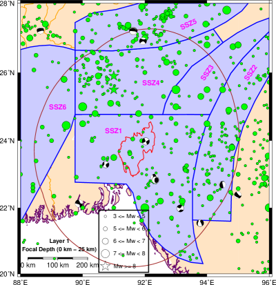
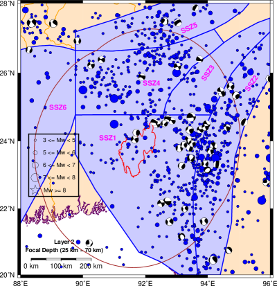
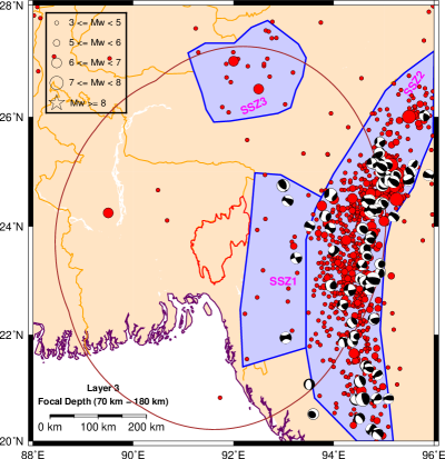
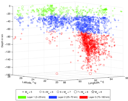
Figure 4: Seismogenic source zones in the study area for all the three Layers along with the 3D depth-section of the main shocks.

A SSZ is considered as an area of diffused seismicity with distinctly different seismogenic potential in terms of the maximum magnitude as well as the occurrence rate of earthquakes in different magnitude ranges. Considering the highly complex spatial distribution and correlation of seismic activity with the tectonic features in the study area, six broad SSZs have been identified for each hypo-central Layer $1$ and $2$ and three SSZs for hypo-central Layer $3$ as shown in Figure 4.

SSZs for Hypo-central Layers 1 and 2

The geometrical coverage of SSZs for Layer $1$ and $2$ are similar. The SSZ$1$ is occupied by frontal Indo-Burma fold belt in the east having lower level of seismicity. The northern part of Bengal Basin is covered in the west. The central part, occupied by N-S trending Tripura-Cachar Fold Belt, constitutes a domain of the upper territory Surma Basin belonging to the periphery of the Indo-Burma orogen. The state boundary of Tripura lies in this zone. The SSZ$2$ encompasses intense seismicity related to the Territory fold thrust belt of the Indo-Burma Arc caused by the subduction of the Indian plate below the Burmese plate. The SSZ$3$ lies southeast of Brahmaputra Basin. The foredeep exposes a narrow belt of imbricate thrust slices, the Shuppen Belt. This belt is delineated on the west by Naga Thrust and on the east by Haflong-Disang Thrust. The SSZ$4$ is seismically active which encompasses mainly Shilling Plateau and part of the Brahmaputra valley in the northeast. The northern margin of the Sillong Plateau subsided step wise to form the basement for the deposition of upper territory sediments and huge pile of alluvium in the Brahmaputra foredeep extending up to Himalayan frontal belt. To the south and east the plateau terminates along Haflong-Disang Thrust. The SSZ$5$ forms the easternmost segment of Himalaya, consists of major thrusts like Main Central Thrust (MCT), Main Boundary Thrust (MBT), and Main Frontal Thrust (MFT), along with several secondary thrusts and transverse tectonic features. The SSZ$6$ consists of the Indo Gangetic plains including Himalayan foredeep and shows somewhat subdued seismic activity.

SSZs for Hypo-central Layer $3$

The SSZ$1$ encompasses low magnitude deep events in the frontal Indo-Burma fold belt. The SSZ$2$ includes intense seismicity related to the Tertiary fold - thrust belt of the Indi-Burma Arc caused by the subduction of the Indian plate below the Burmese plate and the events have deeper focal depths. The SSZ$3$ includes low magnitude deep events from northern part of Shillong Plateau and Eastermost segment of Himalaya consists of MCT, MBT and MFT.

3.3 Catalogue Completeness

It is recognized that earthquake data in the catalogue are generally incomplete for smaller magnitude earthquakes in the early time due to inadequate instrumentation. However, due to short return periods of smaller magnitude, their occurrence rates can be evaluated even from recent data, say, approximately for last $25$ years. However, to have a reliable estimate for the occurrence rates of larger magnitude earthquakes with long return period, the data for a much longer period need to be considered. Failure to correct for data incompleteness may result in underestimation of the mean rates of occurrence of earthquake. The correction can be done by identifying the time period of complete data for a pre-defined magnitude ranges. Reliable mean rates of occurrence of earthquake for the said magnitude ranges can then be computed from the complete data. Stepp (1972) proposed a statistical method to calculate the period of completeness and this method has been followed in the present analysis to determine the period of completeness. Stepp suggested that if the earthquakes in a catalogue are reported completely, they will follow a Poissonian distribution with constant occurrence rates. If $R(M)$ is the average number of events per year for a specific magnitude range centered about $M$ for a time interval of $T$ years, the standard deviation $S_{R}$ of of $R(M)$ is given by

$$S_{R}=\sqrt{R(M)/T}$$ (2)

The stationarity of $R(M)$ guarantees that $S(R)$ behaves as $1/\sqrt{T}$. From the plot of $S(R)$ versus $1/\sqrt{T}$, known as ’completeness plot’, the period of completeness is determined by a marked deviation of of the $S(R)$ values from the linearity of the $1/\sqrt{T}$ slope. The period of completeness becomes successively longer with higher magnitude range. Typical completeness plots for SSZs $1$ and $5$ in Layer $1$, SSZ $1$ in Layer $2$ and SSZ $2$ in Layer $3$ are shown in Figure 5.

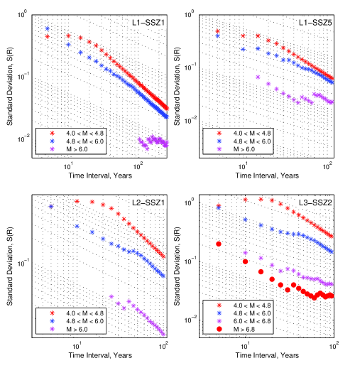
Figure 5: Typical completeness plots for SSZs $1$ and $5$ in Layer $1$, SSZ $1$ in Layer $2$ and SSZ $2$ in Layer $3$.

3.4 Maximum Earthquake Prognosis

The maximum earthquake ($M_{\tt max}$) is the largest seismic event characteristic of the terrain under seismotectonic and stratigraphic conditions. There are a number of methods for determining $M_{\tt max}$ values (Wells and Coppersmith, 1994; Kijko, 2004; Kijko and Graham, 1998) and a certain degree of subjectivity is always associated with each method (Bollinger et al., 1992). For example, Wells and Coppersmith (1994) method needs the fault rupture length of the future earthquakes to be specified and this cannot be determined with any confidence due to lack of scientific basis. In the present study, a maximum likelihood method for maximum earthquake estimation, known as Kijko-Sellevoll-Bayesian (KSB) method, has been adopted for its wide acceptability and sound mathematical background behind it. From the knowledge of the Gutenberg-Richter (GR) probability distribution function (PDF), it is possible to construct the Bayesian version of the Kijko-Sellevoll (KS) estimator of $M_{\tt max}$ (Kijko and Singh, 2011) and the KSB estimator of $M_{\tt max}$ can be calculated by iterative process. Maximum earthquake prognosis has been performed for all the SSZs of all the three layers.

3.5 Estimation of Seismicity Parameters

The evaluation of seismicity parameters is considered to be the most important for hazard estimation. Earthquake occurrences across the the globe are accepted to follow an exponential distribution, given by Gutenberg and Richter (1944) as

$$\log N(M)=a-bM$$ (3)

where $N(M)$ is the mean annual rate of exceedance for magnitude $M$, $i.e$, cumulative number of events with magnitude equal to or greater than $M$. The value of $10^{a}$ is the mean yearly number of earthquakes of magnitude equal to or greater than zero and $b$ (or the $b$ value) describes the relative likelihood of large and small earthquakes. The $a$ and $b$ values are generally obtained by regression analysis of data available for a SSZ of interest. The standard Gutenberg-Richter (GR) relation covers an infinite range of magnitude ranging from $-\infty$ to $+\infty$. For engineering purposes, the effects of very small earthquakes are of little interest and it is common to disregard those that are not capable of causing significant damage (Kramer, 2013). It is therefore necessary to put a lower bound, $i.e$, to consider a lower threshold ($M_{\tt min}$) on the magnitude. At the other end of the magnitude scale, the standard GR law predicts nonzero mean rates of exceedance for magnitude up to infinity. However, there is always an upper bound magnitude or a maximum magnitude ($M_{\tt max}$) associated with all the SSZs. With the imposition of a lower bound and an upper bound magnitude, the GR law is modified to a truncated exponential distribution in the magnitude range $M_{\tt min}$ to $M_{\tt min}$ and is given by (Cornell and Vanmarcke, 1969)

$$N(M)=N(M_{\tt min})\frac{e^{-\beta(M-M_{\tt min})}-e^{-\beta(M_{\tt max}-M_{\tt min})}}{1-e^{-\beta(M_{\tt max}-M_{\tt min})}},~{}M_{\tt min}<M<M_{\tt max}$$ (4)

where $\beta=b\ln 10$. Although the choice of $M_{\tt min}$ is not crucial in Eqn. 4, a suitable $M_{\tt min}$ is necessary for computation of hazard (Bommer and Crowley, 2017). $M_{\tt min}$ is taken as $4.0$ in the present study. The GR relationship for a SSZ is fitted using the maximum likelihood method of Weichert (1980) by first identifying the periods of completeness for different magnitude ranges. As the number of events in SSZ $6$ of Layer $2$ is very less, SSZ $5$ and $6$ of Layer $2$ are merged together to get a good fit by the bounded recurrence law. The bounded recurrence law of Eqn. 4 cannot represent the magnitude-frequency dependence of SSZ $4$ of both Layer $1$ and Layer $2$ well. Therefore a more complex recurrence law, known as characteristic earthquake recurrence law developed by Youngs and Coppersmith (1985) is applied for those two SSZs. The characteristic earthquake model predicts higher rates of exceedance at magnitudes near the characteristic earthquake magnitude and lower rates at lower magnitudes. The seismicity parameters estimated by the applicable recurrence relationship for all the polygonal SSZs in different Layers are listed in Table 2 and the magnitude-frequency distribution plots in each of the SSZs in different Layers are shown in Figure 6.

Table 2: Estimated seismicity parameters for all the polygonal SSZs

	SSZ(s)	$b$-value(s)	$a$-value(s)	$M_{\tt max}$	$M_{\tt max}^{\tt obs}$
	1	1.00 $\pm$ 0.07	4.42	7.96 $\pm$ 0.50	7.53
	2	0.92 $\pm$ 0.08	4.02	6.88 $\pm$ 0.30	6.71
Layer 1	3	0.60 $\pm$ 0.12	2.18	7.90 $\pm$ 0.56	7.40
	4	0.80 $\pm$ 0.07	3.40	8.38 $\pm$ 0.46	8.00
	5	0.82 $\pm$ 0.08	3.71	8.06 $\pm$ 0.44	6.72
	6	0.72 $\pm$ 0.18	2.09	8.72 $\pm$ 0.84	7.92
	1	1.04 $\pm$ 0.06	4.97	7.88 $\pm$ 0.54	7.40
	2	0.92 $\pm$ 0.06	4.46	7.46 $\pm$ 0.35	7.21
Layer 2	3	0.76 $\pm$ 0.13	3.04	6.49 $\pm$ 0.37	6.22
	4	0.92 $\pm$ 0.07	4.28	7.40 $\pm$ 0.39	7.10
	5+6	0.86 $\pm$ 0.01	3.85	5.92 $\pm$ 0.27	5.82
	1	0.60 $\pm$ 0.13	2.19	7.17 $\pm$ 0.71	6.51
Layer 3	2	0.97 $\pm$ 0.03	5.24	7.35 $\pm$ 0.29	7.20
	3	0.56 $\pm$ 0.28	1.72	5.32 $\pm$ 0.39	5.02

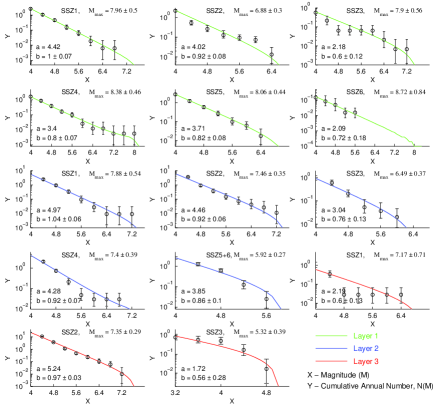
Figure 6: Magnitude-frequency distribution plots for main shocks in each of the polygonal SSZs in all the three Layers.

3.6 Smooth-gridded Seismicity

The seismogenic source is formulated with two schemes, namely smooth-gridded seismicity and uniform-seismicity areal zones (or uniformly smoothed). The former entails spatially varying annual activity rates while $b$-value and $M_{\tt max}$ remain fixed within the source zones. This assumes $b$-value and activity rate to be uncorrelated and a non-uniform distribution of earthquake probability within a zone (Nath and Thingbaijam, 2012). On the other hand, the uniform areal seismicity postulates each point within the zone to have equal probability of earthquake occurrences.

The contribution of background events for hazard perspective is calculated using smooth-gridded seismicity model. It allows modeling of discrete earthquake distributions into spatially continuous probability distributions. The technique given by Frankel (1995) is employed for this purpose in the present study. The technique has been previously employed by several researchers (Frankel et al., 2002; Stirling et al., 2002; Lapajne et al., 2003; Jaiswal and Sinha, 2007; Maiti et al., 2017; Nath and Thingbaijam, 2012). In the present analysis, the study region is gridded at a regular interval of $0.05\degree$$\times$$0.05\degree$. The smoothened function is given as follows:

$$N_{i}(m_{r})=\frac{\sum\limits_{j}n_{j}(m_{r})e^{-(d_{ij}/c})^{2}}{\sum\limits_{j}e^{-(d_{ij}/c})^{2}}$$ (5)

where $n_{j}(m_{r})$ is the number of events with magnitude $\geq m_{r}$, $d_{ij}$ is the distance between $i^{th}$ and $j^{th}$ cells and $c$ denotes the correlation distance which characterizes uncertainty in the epicentral location and is assumed to be $50$ km in the present analysis. The sum is calculated in cells $j$ within a distance of $3c$ of cell $i$. The annual activity rate $\lambda_{m_{r}}$ is computed as $N_{i}(m_{r})/T$ where $T$ is the (sub)catalogue period for threshold magnitude $4.0$ $M_{W}$. The subcatalogue for the threshold magnitude $4.0$ $M_{W}$ covers the period $1988-2020$. The smooth-gridded seismicity for threshold magnitude $4.0$ $M_{W}$ for all the Layers are depicted in Figure 7. From the smooth-gridded seismicity analysis, the areas of probable asperities can be identified (Maiti et al., 2017).

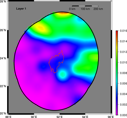
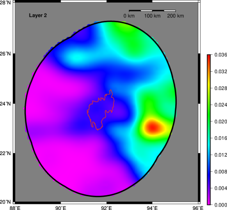
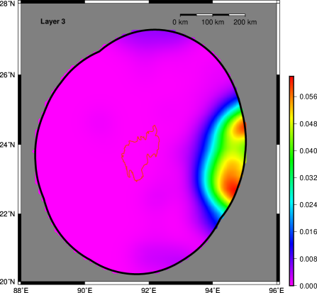
Figure 7: Smooth-gridded seismicity analysis for threshold magnitude $4.0$ $M_{W}$ for all the three Layers.

3.7 Selection of GMPEs

Appropriate selection and ranking of GMPEs against recorded strong motion data are critical for a successful logic tree implementation in the PSHA for incorporating the epistemic uncertainties. A quantitative evaluation of the performance of the selected GMPEs against the observation (the recorded strong motion data) is required for this purpose. To quantify the level of agreement between the observations and the predictions, a number of statistical measures of the goodness-of-fit of an equation to a set of data are calculated in the present analysis following the approach proposed by Scherbaum et al. (2004). This quantitative suitability is often referred to as “efficacy test” of a GMPE for a particular region. These goodness-of-fit measures include mean, median and standard deviation of the normalized residual as well as the median values of the likelihood parameter after Scherbaum et al. (2004). The normalized residual is given by

$$Z=\frac{\log(\text{GM})_{\tt obs}-\log(\text{GM})_{\tt predicted}}{\sigma_{\tt T}}$$ (6)

where $(\text{GM})_{\tt obs}$ and $(\text{GM})_{\tt predicted}$ are the observed and the predicted ground motions and $\sigma_{\tt T}$ is the total standard deviation of the GMPE used. So normalized residual ($Z$) represents the distance of the data from the logarithmic mean measured in units of $\sigma_{\tt T}$. The likelihood parameter is calculated as

$$LH(|Z|)=Erf(\frac{|Z|}{\sqrt{2}},\infty)=\frac{2}{\sqrt{2\pi}}\int_{|Z|}^{\infty}exp\left(\frac{-Z^{2}}{2}\right)dZ$$ (7)

where $Erf$ is the error function. For samples drawn from a normal distribution with unit standard deviation, the values of $LH$ are evenly distributed between $0$ and $1$ and the median value is about $0.5$ (Scherbaum et al., 2004). Ideally, the normalized residual should be normally distributed with zero mean and unit standard distribution. Hence, central tendency measures (Mean $Z$ and Median $Z$) close to zero indicate that the equation is unbiased and the standard deviation of the residual (Std $Z$) close to $1$ indicates that the standard deviation of the GMPE adequately captures that of the recorded data. A median value of the likelihood parameter (Med. $LH$) indicates that the GMPE matches the data in terms of both mean and standard deviation (Arango et al., 2012).

Based on the values of Mean $Z$, Median $Z$, Std $Z$ and Med. $LH$, Scherbaum et al. (2004) defined four categories of ranking of GMPEs. The values of the parameters for deciding the rank of a GMPE are given in Table 3.

Table 3: Values of different parameters for deciding the rank of a GMPE

Mean $Z$	Median $Z$	Std $Z$	Med. $LH$	Rank
$<$ 0.25	$<$ 0.25	$<$ 1.125	$>$ 0.4	A (high capability)
$<$ 0.50	$<$ 0.50	$<$ 1.250	$>$ 0.3	B (medium capability)
$<$ 0.75	$<$ 0.75	$<$ 1.500	$>$ 0.2	C (low capability)
		All other combinations
		of parameters		D (unacceptable capability)

The efficacy test was performed for a number of GMPEs corresponding to recorded earthquake in each Layer. Owing to limited available strong-motion data, $85$ three-component strong-motion accelerograms (A total of $190$ horizontal accelerograms) from $8$ earthquakes of different hypo-central depths have been considered for this purpose. Out of these $190$ accelerograms, $44$ accelerograms belong to Layer $1$, $72$ accelerograms belong to Layer $2$ and $74$ accelerograms belong to Layer $3$. The strong-motion data, used for performing the efficacy test of GMPEs, have been downloaded from Center for Engineering Strong Motion Data (https://www.strongmotioncenter.org). The details of the earthquakes considered are summarized in Table 4.

Table 4: Details of the earthquakes considered for performing the efficacy test

Name of	Date	Lat ($\degree N$)	Lon ($\degree E$)	$M$	$H$	No. of
earthquake	(dd/mm/yy)				(km)	records
$\underline{Layer1}$
1. Sikkim	18/09/2011	27.723	88.064	6.8 $M_{W}$	10	5
2. Indo-Bangladesh	06/02/1988	24.688	91.570	5.8 $M_{S}$	15	17
$\underline{Layer2}$
3. Indo - Bangladesh	08/05/1997	24.894	92.250	6.0 $M_{W}$	34	11
4. Indo - Bangladesh	10/09/1986	23.385	92.077	4.5 $M_{S}$	43	12
5. Indo - Burma	18/05/1987	25.271	94.202	5.9 $M_{S}$	49	13
$\underline{Layer3}$
6. Indo - Burma	06/08/1988	25.149	95.127	7.2 $M_{S}$	90	17
7. Indo - Burma	06/05/1995	24.987	95.127	6.4 $M_{W}$	117	09
8. Indo - Burma	09/01/1990	24.713	95.240	6.1 $M_{W}$	119	11

Based on the suitability test, discussed above, regional and global GMPEs have been selected for the estimation of seismic hazard of the region. The selected GMPEs with the references and codes in the brackets are given in Table 5

The comparisons of the histograms of the normalized residual values (as obtained from Eqn. 6) and the corresponding approximation by the normal distribution (continuous curve) along with the standard normal distribution (dashed curve) for three most suitable GMPEs for each Layer are plotted in the left sides of each sub-figure of Figure 8.

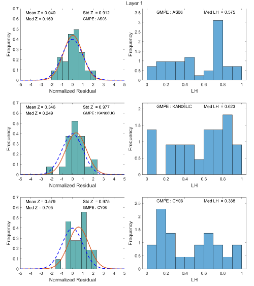
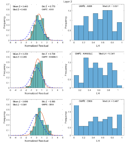
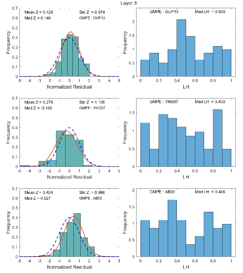
Figure 8: Left side of each sub figure: Comparison of the distributions of normalized residuals and the best-fit normal distributions (continuous curve) with the standard normal distribution (dashed curves) for the selected GMPEs with the mean, median and standard deviation of the normalized residual indicated for all the three Layers. Right side of each sub figure: Corresponding histograms of the likelihood values with the median of LH indicated for all the three Layers.

The mean, median and standard deviation of the normalized residual ($Z$) are also indicated for each case. The corresponding right sides of each sub-figure of Figure 8 plot the histograms of the $LH$ values (as obtained from Eqn. 7), with the corresponding median values indicated for each case. Based on the quantitative assessment, the ranking of the selected GMPEs has been decided. After that the weight factor to each GMPE for each Layer has been decided. The higher the ranking of a GMPE, the more is the weight factor. Therefore, from the set of GMPEs selected for each Layer, the highest ranking GMPE has been assigned more weight and the lowest ranking GMPE has been assigned less weight for the implementation of logic tree approach. The ranking of the selected GMPEs and the corresponding weight factor for each layer are summarized in Table 5. For computations of seismic hazard from the deep-focused earthquakes in Layer $3$, the GMPEs used in Layer $2$ have been employed with the same weight factors as that of Layer $2$.

Table 5: Selected GMPEs used in the study along with their ranking and weight factor

	Name GMPEs with reference(s)	Rank	Weight factor
	Abrahamson and Silva (2008) (AS08)	A	0.5
Layer 1	Kanno et al. (2006) (KAN06UC)	B	0.3
	Chiou and Youngs (2008) (CY08)	C	0.2
	Abrahamson and Silva (2008) (AS08)	B	0.4
Layer 2	Kanno et al. (2006) (KAN06LC)	B	0.4
	Campbell and Bozorgnia (2008) (CB08)	C	0.2
	Gupta (2010) (GUP10)	A	0.5
Layer 3	Youngs et al. (1997) (YNG97)	B	0.3
(subduction)	Atkinson and Boore (2003) (AB03)	C	0.2

3.8 Computation of Hazard

The seismic hazard at a particular site is usually quantified in terms of level of ground motion. Seismic hazard can be obtained for individual SSZ and then combined to express the aggrerate hazard at a particular site. The methodology for PSHA incorporates how often annual rate of ground motion exceeds a specific value for different return periods of the hazard at a particular site of interest. The probability of exceeding a particular value of $y^{*}$ of a ground motion parameter $Y$ is calculated for one possible earthquake (of a particular magnitude) at one possible source locations (source-to-site distance) and then multiplied by the probability that the earthquake of that particular magnitude would occur at that particular location. The process is then repeated for all possible magnitudes and locations with the probabilities of each summed.

For a given earthquake occurrence, the probability that a ground motion parameter $Y$ will exceed a particular value $y^{*}$ can be computed using the total probability theorem (Kramer, 2013)

$$P\left[Y>y^{*}\right]=P\left[Y>y^{*}|\bf{X}\right]P\left[\bf{X}\right]=\int P\left[Y>y^{*}|\bf{X}\right]f_{x}\left(\bf{X}\right)dx$$ (8)

where $\bf{X}$ is a vector of random variables that influences $Y$. For the purpose of computing seismic hazard, the quantities in $\bf{X}$ are limited to magnitude ($M$) and distance ($R$). Assuming that $M$ and $R$ are independent, the probability of exceedance can be written as

$$P\left[Y>y^{*}\right]=\iint P\left[Y>y^{*}|m,r\right]f_{M}(m)f_{R}(r)~{}dm~{}dr$$ (9)

where $P\left[Y>y^{*}|m,r\right]$ is obtained from the predictive relationship and $f_{M}(m)$ and $f_{R}(r)$ are the probability density functions (pdf) for $M$ and $R$ respectively.

If the site of interest is in a region of $N_{s}$ SSZs, each of which has an average rate of threshold magnitude exceedance ( or annual activity rate) $\lambda_{i}$, the total average exceedance rate for the region is given by

$$\nu_{y^{*}}=\sum_{i}^{N_{s}}\lambda_{i}\iint P\left[Y>y^{*}|m,r\right]f_{Mi}(m)\,f_{Ri}(r)\,dm\,dr$$ (10)

The integral 10 cannot be evaluated analytically for virtually all realistic PSHAs. Numerical integration is therefore required. The approach, generally employed, is to discretize the possible ranges of magnitude and distance into $N_{M}$ and $N_{R}$ segments, respectively. The average exceedance rate can then be estimated by

$$\nu_{y^{*}}=\sum_{i=1}^{N_{s}}\sum_{j=1}^{N_{M}}\sum_{k=1}^{N_{R}}\lambda_{i}P\left[Y>y^{*}|m_{j},r_{k}\right]f_{Mi}(m_{j})\,f_{Ri}(r_{k})\,\Delta m\,\Delta r$$ (11)

This is equivalent to assuming that each SSZ is capable of generating $N_{M}$ different earthquakes of magnitude $m_{j}$ at $N_{R}$ different source-to-site distances $r_{k}$. Eqn. 11 is then equivalent to

$$\nu_{y^{*}}=\sum_{i=1}^{N_{s}}\sum_{j=1}^{N_{M}}\sum_{k=1}^{N_{R}}\lambda_{i}P\left[Y>y^{*}|m_{j},r_{k}\right]P\left[M=m_{j}\right]P\left[R=r_{k}\right]$$ (12)

The reciprocal of $\nu_{y^{*}}$ gives the return period for the ground motion parameters $y^{*}$. The probability of exceedance of $y^{*}$ in finite time intervals (say, for an exposure period $T$) can be estimated from the Poisson model

$$P\left[Y_{T}>y^{*}\right]=1-e^{-\lambda_{y^{*}}T}$$ (13)

The foregoing computational technique for PSHA is implemented for all the grid points (sites) at engineering bedrock level ($V_{S30}\sim 760\,m/s$) for $2\%$ and $10\%$ probabilities of exceedance in an exposure period of $50$ years. This corresponds to return periods of $475$ years and $2475$ years respectively.

The different distance parameters like rupture distance ($R_{rup}$), horizontal distance to top edge of the rupture ($R_{x}$) etc, required for implementing the GMPEs, have been determined by using the framework presented by (Kaklamanos et al., 2011) for estimating unknown input parameters.

A logic tree framework approach has been adopted for the computation of hazard at each site to incorporate multiple models in source considerations and GMPEs. Figure 9 depicts a logic tree formulation at a site. In the present study, since the seismogenic source framework has been formulated with two schemes, namely, smooth-gridded seismicity and uniform-seismicity areal zones, both has been collectively assigned weight factor equal to $0.5$. The hazard distributions are computed for the SSZs at each depth-section separately and thereafter added.

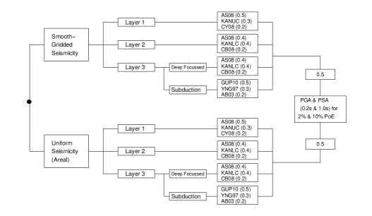
Figure 9: The logic tree framework employed in the present study

4 Result and Discussion

The hazard distributions are estimated for the seismogenic source zones at three Layers corresponding to hypo-central depth ranges of 0 - 25 km, 25 - 70 km and 70 - 180 km separately and added thereafter. The seismogenic source zones include conventional area sources of spatially uniform seismicity (uniform seismicity areal zones) as well as spatially non-uniform seismicity (smooth- gridded seismicity). The results obtained from both the uniform and the non-uniform seismicity are integrated with equal weight factor 0.5 to establish the overall hazard distribution in Tripura State at engineering bedrock level. The peak ground acceleration (PGA) and 5$\%$ damped pseudo spectral acceleration (PSA) at 0.2 s and 1.0 s for all the sites (grid points) for 10$\%$ and 2$\%$ probabilities of exceedance (PoE) in an exposure period of 50 years (corresponding to return periods of 475 years and 2475 years) have been computed at engineering bedrock level conforming to $V_{S30}=760$ m/s. The return period of 2475 years represent the maximum considered earthquake (MCE) condition while the return period of 475 years represents the design basis earthquake (DBE) condition (ASCE, 2010; ICC, 2009). PSA at 0.2 s and 1.0 s are selected because those are frequently used as corner spectral periods to construct a smooth design spectrum for structural designi (Maiti et al., 2017).

The seismic hazard maps in terms of the spatial distribution of PGA and PSA at 0.2 s and 1.0 s, respectively for both DBE and MCE conditions at engineering bedrock is presented in Figure 10. The left side plots in Fig. 10 shows the hazard maps for a return period of 475 years while the right-side plots shows the same for a return period of 2475 years. For design purpose, 10$\%$ PoE in 50 years are considered to be more appropriate and ideally used.

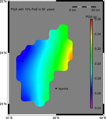
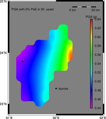
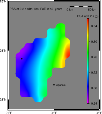
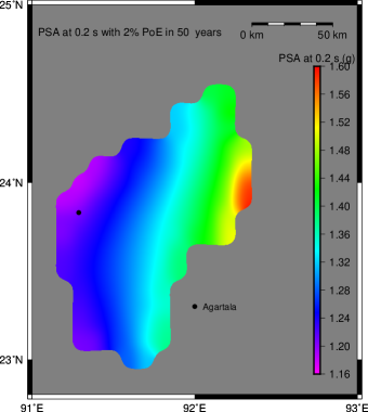
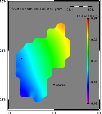
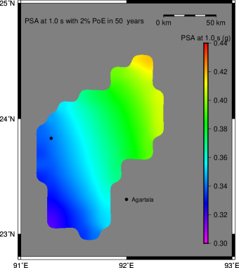
Figure 10: Seismic hazard distribution map of Tripura in terms of PGA and PSA at 0.2 s and 1.0 s for 10$\%$ PoE in 50 years (left) and 2$\%$ PoE in 50 years (right) at firm rock site conditions.

The PGA distribution for 10$\%$ PoE in 50 years at firm rock site shows variation from 0.2602 g to 0.3461 g for Tripura. The State capital Agartala has a hazard level to the tune of 0.264 g. The PSA at 0.2 s exhibits a spatial variation between 0.6546 g to 0.8531 g while for 1.0 s, it ranges from 0.1745 g to 0.2298 g. The present seismic hazard analysis represents significant improvements over the deterministic zonation of BIS (1893-2016) and captures the local variation in seismic hazard well whereas BIS (1893-2016) suggested to consider an uniform hazard value. The treatment to seismicity data in different hypo-central depth ranges together with improved seismogenic source zonations and logic tree approach has produced seismic hazard level different from those reported in earlier studies by other researchers (Bhatia et al., 1999; BIS, 1893-2016; Sharma and Malik, 2006; Iyengar et al., 2011; Nath and Thingbaijam, 2012; Das et al., 2016). A comparison of the computed PGA values for 10$\%$ PoE in 50 years with other studies at the State capital Agartala has been shown in Table 6

Table 6: Comparison of computed PGA with other studies for 10$\%$ PoE in 50 years at Agartala city

Name of the studies	DBE level PGA
Bhatia et al. (1999)	0.45
BIS (1893-2016)	0.18
Sharma and Malik (2006)	0.30
Iyengar et al. (2011)	0.18
Nath and Thingbaijam (2012)	0.50
Das et al. (2016)	0.217
Present Study	0.264

The variation in PGA distribution for 2$\%$ PoE in 50 years ranges from 0.4508 g to 0.6234 g while PSA at 0.2 s and 1.0 s shows a variation of 1.1780 g to 1.5785 g and 0.3196 g to 0.4184 g, respectively. In the present study, north, east, northeastern and southeastern parts of Tripura have been found to show high hazard compared to other parts of the State. The hazard maps obtained from the study is also able to exhibit a significant local variation in seismic hazard.

5 Conclusion

The aim of the present study was to obtain the probabilistic seismic hazard map of Tripura in engineering bed rock level in terms of PGA and 5$\%$ damped PSA at 0.2 s and 1.0 s for return periods of 475 years and 2475 years. An updated and comprehensive earthquake catalogue has been employed to prepare the hazard maps. The catalogue is then first homogenized into an unified moment magnitude and then declustered to remove the aftershocks and foreshocks. In our opinion, the final results presented in the study show significant improvements over the earlier studies. This can be attributed to several factors - (a) A layered seismogenic source framework and smooth-gridded seismicity models conforming to the variation of seismo-tectonic attributes with hypo-central depth have been considered, (b) multiple GMPEs, selected after performing a thorough quantitative assessment with the recorded strong motion data, have been employed, thus accounting for the epistemic uncertainties, (c) the computations of hazard have been carried out in a finer resolution of grid intervals and (d) the earthquake database has been updated up to the year 2020. The seismic hazard maps prepared at the engineering bedrock level exhibit a significant spatial variation which is consistent with the trends of the major tectonic features and the past seismicity as well. The minimum and maximum PGA for 10$\%$ PoE in 50 years (corresponding to return period of 475 years) are found to be 0.2602 g and 0.3461 g, respectively. The same for 2$\%$ PoE in 50 years (corresponding to return period of 2475 years) are reported as 0.4508 g and 0.6234 g, respectively. As the seismic hazard analysis is considered to be an integral part of the earthquake-induced disaster mitigation practices, we hope that the present study is important towards updating the regional building code provisions for earthquake-resistant design and construction of structures in this high seismicity region.

Declaration of Conflicts of Interest and Funding

The authors have no conflicts of interest to declare that are relevant to the content of this article. No funding was received for conducting this study.