The a posteriori error estimates and an adaptive algorithm of the FEM for transmission eigenvalues for anisotropic media

Abstract

The transmission eigenvalue problem arising from the inverse scattering theory is of great importance in the theory of qualitative methods and in the practical applications. In this paper, we study the transmission eigenvalue problem for anisotropic inhomogeneous media in $\Omega\subset\mathbb{R}^{d}\,(d=2,3)$. Using the $\mathbb{T}$-coercivity and the spectral approximation theory, we derive an a posteriori estimator of residual type and prove its effectiveness and reliability for eigenfunctions. In addition, we also prove the reliability of the estimator for transmission eigenvalues. The numerical experiments indicate our method is efficient and can reach the optimal order $DoF^{-2m/d}$ by using piecewise polynomials of degree $m$ for real eigenvalues.

Key words. transmission eigenvalues, $\mathbb{T}$-coercivity, a posteriori error estimates, adaptive algorithm.

1 Introduction

The transmission eigenvalue problem arising from the inverse scattering theory for inhomogeneous media is of great importance in the proof of the unique determination of an inhomogeneous media, and transmission eigenvalues can be reconstructed from the scattering data and used to obtain physical properties of the unknown target [1, 2, 3]. So, the computation for transmission eigenvalues becomes an attractive issue in academic circle since the first paper by Colton, Monk and Sun [4].
In this paper, we consider the following transmission eigenvalue problem: Find $\mathrm{k}\in\mathbb{C},(w,v)\in H^{1}(\Omega)\times H^{1}(\Omega)$ such that

$$\left\{\begin{array}[]{ll}\nabla\cdot(A\nabla w)+\mathrm{k}^{2}nw=0{}{}&\mathrm{in}\,~{}\Omega,\\ \triangle v+\mathrm{k}^{2}v=0{}{}&\mathrm{in}\,~{}\Omega,\\ w-v=0{}{}{}{}{}{}{}{}{}{}{}{}{}&\mathrm{on}\,~{}\partial\Omega,\\ \frac{\partial w}{\partial\nu_{A}}-\frac{\partial v}{\partial\nu}=0{}{}{}{}{}{}{}{}{}{}{}{}{}&\mathrm{on}\,~{}\partial\Omega,\end{array}\right.$$ (1.1)

where $\Omega\subset\mathbb{R}^{d}\,(d=2,3)$ is a bounded domain with Lipschitz boundary $\partial\Omega$, $A(x)$ is a real-valued symmetric matrix function and $n(x)$ is the index of refraction, $\nu$ is the unit outward normal to the boundary $\partial\Omega$ and $\frac{\partial w}{\partial\nu_{A}}=\nu\cdot(A\nabla w)$.
As for the problem (1.1), most existing numerical researches only cover the isotropic media, i.e., $A(x)=I$ (see [5, 6] and the references therein, and see articles [7, 8, 9, 10, 11, 12, 13, 14, 15, 16, 17, 18, 19, 20] and so on). In the case of anisotropic inhomogeneous media ($A(x)\not=I$), due to the complexity of the problem being neither elliptic nor self-adjoint, few numerical treatments have been addressed. Ji et al. [21] first propose a mixed finite element method and a multilevel method but without convergence proof, Xie et al. [22] proved the convergence of the mixed finite element method and gave a multilevel correction method using $\mathbb{T}$-coercivity, and Gong et al. [23] formulated the problem as a eigenvalue problem of a holomorphic Fredholm operator function and proposed a finite element discretization.
When studying the transmission equation/eigenvalue problems, the $\mathbb{T}$-coercivity is important and useful (see [24, 25, 26, 27, 28, 22]) which is equivalent to the $\inf$-$\sup$ condition (see [29]). In this paper, using the $\mathbb{T}$-coercivity we study the a posteriori error estimates of residual type of mixed finite element method and an adaptive method for the problem (1.1) when $A(x)\not=I$, and our work has the following features:
(1) Under the adaptive computation mode, it generally needs to solve the primal and the adjoint problems at the same time when solving non-selfadjoint eigenvalue problems (see, e.g., [30, 31]). Based on the mixed formulation which was proposed in [25], we show that $\lambda$ is the eigenvalue of the primal eigenvalue problem with the corresponding generalized eigenfunction $\mathbf{U}^{j}$ of order $j\geq 1$ if and only if $\lambda$ is the eigenvalue of the adjoint eigenvalue problem and $\mathbf{U}^{j}$ is a generalized eigenfunction of order $j\geq 1$ corresponding to $\lambda$ (see Theorem 2.1). Due to this fact, in our adaptive method it has no need to analyze and solve the adjoint eigenvalue problem but the primal problem only.
(2)  Xie and Wu [22] first presented an a priori error estimate of the mixed finite element method in terms of the gap of the generalized eigenfunction space. Based on [22], this paper further studies the a priori error estimate. Note that if $(w,v)$ is the solution of the source problem corresponding to the problem (1.1) then $(w,v)\in H^{1+r}(\Omega)\times H^{1+r}(\Omega)$ (see [32]). However, to the best of our knowledge, the following regularity estimate is not available in general:

$$\|w\|_{H^{1+r}}+\|v\|_{H^{1+r}}\leq C_{\Omega}(\|f\|_{L^{2}(\Omega)}+\|g\|_{L^{2}(\Omega)}),$$ (1.2)

where $(f,g)\in L^{2}(\Omega)\times L^{2}(\Omega)$ is the right-hand side of the source problem and $C_{\Omega}$ is the a prior constant. Hence, we use the approximation property of the finite element space and the fact that the point-wise convergence on a compact set implies the uniform convergence to prove that the discrete solution operator converges to the solution operator according to the operator norm. Then we employ the $\mathbb{T}$-coercivity and the spectral approximation theory to prove that the approximate eigenpairs converge to the exact eigenpairs, and prove the error estimate of eigenfunctions in $L^{2}(\Omega)\times L^{2}(\Omega)$ norm is a small quantity of higher order compared with the error estimate in $H^{1}(\Omega)\times H^{1}(\Omega)$ norm.
(3) In practical finite element computations, it is desirable to carry out the computations in adaptive fashion (see, e.g., [33, 34, 35, 36, 37, 38] and the references cited therein). [28] gave an a posteriori error estimate for the boundary value problem associated with the eigenvalue problem (1.1). Here we propose an a posteriori estimator of residual type for (1.1). Using the $\mathbb{T}$-coercivity we prove the a posteriori error formulas (see Lemma 3.1), and give the global upper bound and the local lower bound for the error of eigenfunctions. In particular, we also prove the reliability of the estimator for transmission eigenvalues. Numerical experiments indicate that our method is efficient and can reach the optimal order $DoF^{-2m/d}$ by using piecewise polynomials of degree $m$ for real eigenvalues.
In this paper, regarding the basic theory of finite element methods, we refer to [39, 40, 41, 42, 43].
Throughout this article, for the sake of simplicity, we write $a\lesssim b$ when $a\leq Cb$ and $a\gtrsim b$ when $a\geq Cb$ for some positive constant $C$ independent of the finite element mesh.

2 Finite element approximation and its a priori error estimates

In this section, we introduce the finite element approximation and its a priori error estimates for (1.1). We assume that there exists a real number $\gamma>1$ such that

$$\xi\cdot A\xi>\gamma|\xi|^{2}\quad\forall\xi\in\mathbb{R}^{d},n(x)>\gamma,\text{~{}a.\,e.}~{}\mathrm{in}\,~{}\Omega.$$ (2.1)

Let $H^{s}(D)$ be the Sobolev space on the domain $D\subseteq\Omega$ with the associated norm $\|\cdot\|_{s,D}$. We omit the subscript $D$ if $D=\Omega$ from the norm notation.

The eigenvalue problem (1.1) can be transformed into the following version: Find $\lambda=\mathrm{k}^{2}+1\in\mathbb{C},(u,w)\in H^{1}(\Omega)\times H^{1}(\Omega)$ such that

$$\left\{\begin{array}[]{ll}-\nabla\cdot(A\nabla w)+n(x)w=\lambda n(x)w{}{}&\mathrm{in}\,\Omega,\\ -\triangle v+v=\lambda v{}{}&\mathrm{in}\,\Omega,\\ w-v=0{}{}{}{}{}{}{}{}{}{}{}{}{}&\mathrm{on}\,\partial\Omega,\\ \frac{\partial w}{\partial\nu_{A}}-\frac{\partial v}{\partial\nu}=0{}{}{}{}{}{}{}{}{}{}{}{}{}&\mathrm{on}\,\partial\Omega.\end{array}\right.$$ (2.2)

Define the function spaces $\mathbb{V}$ and $\mathbb{W}$ as follows:

$$\mathbb{V}=\bigg{\{}\Psi=(\varphi,\psi)\in H^{1}(\Omega)\times H^{1}(\Omega)\,|\,\varphi-\psi\in H_{0}^{1}(\Omega)\bigg{\}},$$ (2.3)

$$\mathbb{W}=L^{2}(\Omega)\times L^{2}(\Omega)$$ (2.4)

and the associated norm is given by

$$\|\Psi\|_{\mathbb{V}}=\bigg{(}\|\varphi\|_{1}^{2}+\|\psi\|_{1}^{2}\bigg{)}^{1/2}\mathrm{and}\,~{}\|\Psi\|_{\mathbb{W}}=\bigg{(}\|\varphi\|_{0}^{2}+\|\psi\|_{0}^{2}\bigg{)}^{1/2},$$

respectively, where $\mathbf{\Psi}=(\varphi,\psi)$.
Then $\mathbb{V}\subset\mathbb{W}$ with a compact imbedding.
For $\mathbf{U}=(w,v),\Psi=(\varphi,\psi)\in\mathbb{V},$ we define two sesquilinear forms

$$a(\mathbf{U},\Psi)=(A\nabla w,\nabla\varphi)_{0}+(n(x)w,\varphi)_{0}-(\nabla v,\nabla\psi)_{0}-(v,\psi)_{0},$$ (2.5)

$$b(\mathbf{U},\Psi)=(n(x)w,\varphi)_{0}-(v,\psi)_{0},$$ (2.6)

where $(w,\varphi)_{0}=\int_{\Omega}w\overline{\varphi}\,\mathrm{d}x$.
It is clear that

$$|a(\mathbf{U},\Psi)|\lesssim\|\mathbf{U}\|_{\mathbb{V}}\|\Psi\|_{\mathbb{V}}\quad\forall\mathbf{U},\Psi\in\mathbb{V},$$ (2.7)

$$|b(\mathbf{U},\Psi)|\lesssim\|\mathbf{U}\|_{\mathbb{W}}\|\Psi\|_{\mathbb{W}}\quad\forall\mathbf{U},\Psi\in\mathbb{W}.$$ (2.8)

Thanks to [25, 22], the variational form associated with (2.2) is given by: Find $\lambda\in\mathbb{C}$ and $\mathbf{U}\in\mathbb{V}$, $\mathbf{U}\neq 0$, such that

$$a(\mathbf{U},\Psi)=\lambda b(\mathbf{U},\Psi)\quad\forall\Psi\in\mathbb{V}.$$ (2.9)

Then the corresponding adjoint eigenvalue problem is: Find $\lambda^{*}\in\mathbb{C}$ and $\mathbf{U}^{*}\in\mathbb{V}$, $\mathbf{U}^{*}\neq 0$, such that

$$a(\Psi,\mathbf{U}^{*})=\bar{\lambda}^{*}b(\Psi,\mathbf{U}^{*})\quad\forall\Psi\in\mathbb{V}.$$ (2.10)

Let $\lambda$ be the eigenvalue of (2.9). From page 683 and page 693 in [39] we know that $\mathbf{U}^{j}$ is a generalized eigenfunction of order $j>1$ corresponding to $\lambda$ if and only if

$$a(\mathbf{U}^{j},\Psi)=\lambda b(\mathbf{U}^{j},\Psi)+\lambda a(\mathbf{U}^{j-1},\Psi)\quad\forall\Psi\in\mathbb{V},$$

where $\mathbf{U}^{j-1}$ is a generalized eigenfunction of order $j-1$ corresponding to $\lambda$. And the eigenfunction is a generalized eigenfunction of order $1$.

Theorem 2.1.

The number $\lambda$ is the eigenvalue of (2.9) and $\mathbf{U}^{j}$ is a generalized eigenfunction of order $j\geq 1$ corresponding to $\lambda$ if and only if $\lambda$ is the eigenvalue of (2.10) and $\mathbf{U}^{j}$ is a generalized eigenfunction of order $j\geq 1$ corresponding to $\lambda$.

Proof.

The proof is completed by induction. Let $\lambda$ be the eigenvalue of (2.9) and $\mathbf{U}$ be a generalized eigenfunction of order $1$ corresponding to $\lambda$. Since $a(\cdot,\cdot)$ and $b(\cdot,\cdot)$ are both self-adjoint, we get

$$a(\Psi,\mathbf{U})=\overline{a(\mathbf{U},\Psi)}=\overline{\lambda b(\mathbf{U},\Psi)}=\overline{\lambda}b(\Psi,\mathbf{U})\quad\forall\Psi\in\mathbb{V}.$$

This shows $\lambda$ is the eigenvalue of (2.10) and $\mathbf{U}$ is a generalized eigenfunction of order $1$ corresponding to $\lambda$.
Suppose that the conclusion 2.1 holds for $j-1$. Let $\mathbf{U}^{j}$ be a generalized eigenfunction of (2.9) of order $j$ corresponding $\lambda$, then

$$a(\mathbf{U}^{j},\Psi)=\lambda b(\mathbf{U}^{j},\Psi)+a(\mathbf{U}^{j-1},\Psi)\quad\forall\Psi\in\mathbb{V}.$$

Again from the fact that $a(\cdot,\cdot)$ and $b(\cdot,\cdot)$ are self-adjoint, we deduce

$$a(\Psi,\mathbf{U}^{j})=\overline{a(\mathbf{U}^{j},\Psi)}=\overline{\lambda b(\mathbf{U}^{j},\Psi)+a(\mathbf{U}^{j-1},\Psi)}$$

$$~{}~{}~{}=\overline{\lambda}b(\Psi,\mathbf{U}^{j})+a(\Psi,\mathbf{U}^{j-1})\quad\forall\Psi\in\mathbb{V}.$$

This indicates $\lambda$ is the eigenvalue of (2.10) and $\mathbf{U}^{j}$ is a generalized eigenfunction of order $j$ corresponding to $\lambda$.
Conversely, we can prove the other part of the theorem is valid. ∎

Remark 2.1.

When $\lambda$ is a complex eigenvalue and $\mathbf{U}$ is an eigenfunction corresponding to $\lambda$, we have

$$\lambda b(\mathbf{U},\mathbf{U})=a(\mathbf{U},\mathbf{U}).$$

Note that $b(\mathbf{U},\mathbf{U})$ and $a(\mathbf{U},\mathbf{U})$ are both real numbers, then there must hold $b(\mathbf{U},\mathbf{U})=0$ and $a(\mathbf{U},\mathbf{U})=0$.

In order to analyze the eigenvalue problem (2.9), we introduce the $\mathbb{T}$-coercivity for the sesquilinear form $a(\cdot,\cdot)$. We use $\mathbb{T}$ to denote an isomorphic operator from $\mathbb{V}$ to $\mathbb{V}$ which is defined as follows:

$$\mathbb{T}\Psi=(\varphi,2\varphi-\psi)\quad\forall\Psi=(\varphi,\psi)\in\mathbb{V}.$$ (2.11)

Thanks to [25, 22], we know that $a(\cdot,\cdot)$ is $\mathbb{T}$-coercive:

$$|a(\Psi,\mathbb{T}\Psi)|\gtrsim\|\Psi\|_{\mathbb{V}}^{2}\quad\forall\Psi=(\varphi,\psi)\in\mathbb{V}.$$ (2.12)

In fact,

$$|a(\Psi,\mathbb{T}\Psi)|=|(A\nabla\varphi,\nabla\varphi)_{0}+(n(x)\varphi,\varphi)_{0}-(\nabla\mathbf{\psi},\nabla(2\varphi-\psi))_{0}-(\mathbf{\psi},2\varphi-\psi)_{0}|$$

$$~{}~{}~{}\geq\gamma\|\varphi\|_{1}^{2}+\|\psi\|_{1}^{2}-2|(\nabla\psi,\nabla\varphi)_{0}|-2|(\psi,\varphi)_{0}|$$

$$~{}~{}~{}\geq(\gamma-\delta^{-1})\|\varphi\|_{1}^{2}+(1-\delta)\|\psi\|_{1}^{2},$$

thus we can choose $\delta\in(1/\gamma,1)$ such that (2.12) holds.
Theorem 1 in [29] and Theorem 1 in [22] show that the $\mathbb{T}$-coercivity of the form $a(\cdot,\cdot)$ is equivalent to the inf-sup condition of the form $a(\cdot,\cdot)$, namely, there hold

$$\inf_{0\neq\Phi\in\mathbb{V}}\sup_{0\neq\Psi\in\mathbb{V}}\frac{|a(\Phi,\Psi)|}{\|\Phi\|_{\mathbb{V}}\|\Psi\|_{\mathbb{V}}}\geq\mu_{a},$$ (2.13)

$$\inf_{0\neq\Phi\in\mathbb{V}}\sup_{0\neq\Psi\in\mathbb{V}}\frac{|a(\Psi,\Phi)|}{\|\Psi\|_{\mathbb{V}}\|\Phi\|_{\mathbb{V}}}\geq\mu_{a},$$ (2.14)

for some positive constant $\mu_{a}$.
Thanks to Section 8 in [39] and Chapter 5 in [44] we know that there are the solution operators $\mathbb{K}:\mathbb{W}\to\mathbb{V}$ and $\mathbb{K}_{*}:\mathbb{W}\to\mathbb{V}$ satisfying

$$a(\mathbb{K}\mathbf{F},\Psi)=b(\mathbf{F},\Psi)\quad\forall\Psi\in\mathbb{V},$$ (2.15)

$$a(\Psi,\mathbb{K}_{*}\mathbf{F})=b(\Psi,\mathbf{F})\quad\forall\Psi\in\mathbb{V},$$ (2.16)

and it is valid that

$$\|\mathbb{K}\mathbf{F}\|_{\mathbb{V}}\lesssim\|\mathbf{F}\|_{\mathbb{W}}\quad\forall\mathbf{F}\in\mathbb{W},$$ (2.17)

$$\|\mathbb{K}_{*}\mathbf{F}\|_{\mathbb{V}}\lesssim\|\mathbf{F}\|_{\mathbb{W}}\quad\forall\mathbf{F}\in\mathbb{W}.$$ (2.18)

Thus, since $\mathbb{V}\subset\mathbb{W}$ with a compact imbedding, $\mathbb{K}:\mathbb{W}\to\mathbb{W}$ is compact and $\mathbb{K}:\mathbb{V}\to\mathbb{V}$ is compact.
From [39], we know that (2.9) and (2.10) have the equivalent operator form

$$\lambda\mathbb{K}\mathbf{U}=\mathbf{U}~{}~{}\mathrm{and}~{}~{}\lambda^{*}\mathbb{K}_{*}\mathbf{U}=\mathbf{U},$$ (2.19)

respectively.
Let $\{\mathcal{T}_{h}\}$ be a family of regular triangulation of $\Omega$ with the mesh diameter $h$, let $S^{h}\subset H^{1}(\Omega)$ be the conforming Lagrange finite element space on $\mathcal{T}_{h}$ which consists of piecewise polynomials of degree $m$. Denote

$$\mathbb{V}_{h}=\{(w_{h},v_{h})\in S^{h}\times S^{h}\,|\,w_{h}=v_{h}~{}\text{on}~{}\partial\Omega\}.$$

Then $\mathbb{V}_{h}\subset\mathbb{V}$.
Thus we also have the following discrete inf-sup conditions:

$$\|\Phi_{h}\|_{\mathbb{V}}\lesssim\sup_{\Psi_{h}\in\mathbb{V}_{h}}\frac{|a(\Phi_{h},\Psi_{h})|}{\|\Psi_{h}\|_{\mathbb{V}}}\quad\mathrm{and}\quad\|\Phi_{h}\|_{\mathbb{V}}\lesssim\sup_{\Psi_{h}\in\mathbb{V}_{h}}\frac{|a(\Psi_{h},\Phi_{h})|}{\|\Psi_{h}\|_{\mathbb{V}}}.$$ (2.20)

The finite element approximation of (2.9) is given by: Find $\lambda_{h}\in\mathbb{C}$ and $\mathbf{U}_{h}\in\mathbb{V}_{h}$, $\mathbf{U}_{h}\neq 0$, such that

$$a(\mathbf{U}_{h},\Psi)=\lambda_{h}b(\mathbf{U}_{h},\Psi)\quad\forall\Psi\in\mathbb{V}_{h}.$$ (2.21)

The finite element approximation of (2.10) is given by: Find $\lambda_{h}^{*}\in\mathbb{C}$ and $\mathbf{U}_{h}^{*}\in\mathbb{V}_{h}$, $\mathbf{U}_{h}^{*}\neq 0$, such that

$$a(\Psi,\mathbf{U}_{h}^{*})=\lambda_{h}^{*}b(\Psi,\mathbf{U}_{h}^{*})\quad\forall\Psi\in\mathbb{V}_{h}.$$ (2.22)

It is clear that Theorem 2.1 also holds for (2.21) and (2.22).
Since (2.20) holds, there are the solution operators $\mathbb{K}_{h}:\mathbb{W}\to\mathbb{V}_{h}$ and $\mathbb{K}_{h*}:\mathbb{W}\to\mathbb{V}_{h}$ satisfying

$$a(\mathbb{K}_{h}\mathbf{F},\Psi)=b(\mathbf{F},\Psi)\quad\forall\Psi\in\mathbb{V}_{h},$$ (2.23)

$$a(\Psi,\mathbb{K}_{h*}\mathbf{F})=b(\Psi,\mathbf{F})\quad\forall\Psi\in\mathbb{V}_{h},$$ (2.24)

and it is valid that

$$\|\mathbb{K}_{h}\mathbf{F}\|_{\mathbb{V}}\lesssim\|\mathbf{F}\|_{\mathbb{W}}\quad\forall\mathbf{F}\in\mathbb{W},$$ (2.25)

$$\|\mathbb{K}_{h*}\mathbf{F}\|_{\mathbb{V}}\lesssim\|\mathbf{F}\|_{\mathbb{W}}\quad\forall\mathbf{F}\in\mathbb{W}.$$ (2.26)

From [39], we know that (2.21) and (2.22) have the equivalent operator form

$$\lambda_{h}\mathbb{K}_{h}\mathbf{U}_{h}=\mathbf{U}_{h}~{}~{}\mathrm{and}~{}~{}\lambda_{h}^{*}\mathbb{K}_{h}^{*}\mathbf{U}_{h}=\mathbf{U}_{h},$$ (2.27)

respectively.
Let $P_{h}:\mathbb{V}\to\mathbb{V}_{h}$ and $P_{h}^{*}:\mathbb{V}\to\mathbb{V}_{h}$ be the projection operators defined by

$$a(\Phi-P_{h}\Phi,\Psi_{h}) =0\quad\forall\,\Psi_{h}\in\mathbb{V}_{h},$$ (2.28)

$$a(\Psi_{h},\Phi-P_{h}^{*}\Phi) =0\quad\forall\,\Psi_{h}\in\mathbb{V}_{h}.$$ (2.29)

Then $\mathbb{K}_{h}=P_{h}\mathbb{K}$ and $\mathbb{K}_{h*}=P_{h}^{*}\mathbb{K}^{*}$.

Lemma 2.1.

Assume that (2.1) is valid, then

$$\|\mathbb{K}_{h}-\mathbb{K}\|_{\mathbb{V}}\to 0~{}as~{}h\to~{}0~{}~{}and~{}~{}\|\mathbb{K}_{h*}-\mathbb{K}_{*}\|_{\mathbb{V}}\to 0~{}as~{}h\to~{}0.$$

Proof.

From $\mathbb{T}$-coercivity of $a(\cdot,\cdot)$ we deduce that

$$\|\Psi-P_{h}\Psi\|_{\mathbb{V}}^{2}\lesssim a(\Psi-P_{h}\Psi,\mathbb{T}(\Psi-P_{h}\Psi))$$

$$~{}~{}~{}=Ca(\Psi-P_{h}\Psi,\mathbb{T}(\Psi-\Phi_{h}))$$

$$~{}~{}~{}\lesssim\|\Psi-P_{h}\Psi\|_{\mathbb{V}}\|\Psi-\Phi_{h}\|_{\mathbb{V}}\quad\forall\Phi_{h}\in\mathbb{V}_{h},$$

thus, from the interpolation estimate we obtain

$$\|\Psi-P_{h}\Psi\|_{\mathbb{V}}\lesssim\inf\limits_{\Phi_{h}\in\mathbb{V}_{h}}\|\Psi-\Phi_{h}\|_{\mathbb{V}}\to 0~{}~{}(h\to 0)\quad\forall\Psi\in\mathbb{V}.$$ (2.30)

Since $\mathbb{K}$ is compact, $\mathbb{K}_{h}=P_{h}\mathbb{K}$ converges to $\mathbb{K}$ in norm $||\cdot||_{\mathbb{V}}$ as $h\to 0$. Similarly, we have $\mathbb{K}_{h*}=P_{h}^{*}\mathbb{K}_{*}$ converges to $\mathbb{K}_{*}$ in norm $||\cdot||_{\mathbb{V}}$ as $h\to 0$. ∎

Suppose that $\lambda$ and $\lambda_{h}$ are the $k$th eigenvalue of (2.9) and (2.21), respectively. Let $q$ and $\alpha$ be the algebraic multiplicity and the ascent of $\lambda$, respectively, $\lambda=\lambda_{k}=\lambda_{k+1}=\cdots=\lambda_{k+q-1}$. Let $M(\lambda)$ be the generalized eigenfunction space of (2.9) corresponding to $\lambda$ and $M_{h}(\lambda)$ be the direct sum of the generalized eigenfunctions corresponding to all eigenvalues of (2.21) that converge to $\lambda$. And let $M^{*}(\lambda)$ be the generalized eigenfunction space of (2.10) corresponding to $\lambda^{*}$. Let $\hat{M}(\lambda)=\{\Psi|\Psi\in M(\lambda),\|\Psi\|_{\mathbb{V}}=1\}$ and $\hat{M}^{*}(\lambda)=\{\Psi|\Psi\in M^{*}(\lambda),\|\Psi\|_{\mathbb{V}}=1\}$. From Theorem 2.1 we know $\lambda^{*}=\lambda$, $M^{*}(\lambda)=M(\lambda)$ and $\hat{M}^{*}(\lambda)=\hat{M}(\lambda)$.
Denote

$$\delta_{h}(\lambda)=\sup_{\mathbf{U}\in\hat{M}(\lambda)}\inf_{\Psi_{h}\in\mathbb{V}_{h}}\|\mathbf{U}-\Psi_{h}\|_{\mathbb{V}},\,\delta_{h}^{*}(\lambda)=\sup_{\mathbf{U}\in\hat{M}^{*}(\lambda)}\inf_{\Psi_{h}\in\mathbb{V}_{h}}\|\mathbf{U}-\Psi_{h}\|_{\mathbb{V}}.$$

Then $\delta_{h}(\lambda)=\delta_{h}^{*}(\lambda)$.
For two closed subspaces $A$ and $B$ of $\mathbb{V}$, we denote

$$\hat{\Theta}(A,B)=\sup_{\Phi\in A,\|\Phi\|_{\mathbb{V}}=1}\inf_{\Psi\in B}\|\Phi-\Psi\|_{\mathbb{V}},\,$$

and define the gap between $A$ and $B$ in norm $\|\cdot\|_{\mathbb{V}}$ as

$$\Theta(A,B)=\max\{\hat{\Theta}(A,B),\hat{\Theta}(B,A)\}.$$ (2.31)

Similarly, we can define the gap $\Theta_{\mathbb{W}}(A,B)$ between two closed subspaces $A$ and $B$ of $\mathbb{W}$ in the sense of norm $\|\cdot\|_{\mathbb{W}}$.
Since (2.7), (2.8), (2.13) and (2.14) hold and $\mathbb{V}\subset\mathbb{W}$ with a compact imbedding, thanks to Theorems 8.1-8.4 in [39] we obtain the following result.

Theorem 2.2.

Assume that $\lambda$ is the $k$th eigenvalue of (2.9), $\hat{\lambda}_{h}=\frac{1}{q}\sum\limits_{j=k}^{k+q-1}\lambda_{j,h}$ denotes the arithmetic mean of $q$ discrete eigenvalues of (2.21) that converge to $\lambda$, and $h$ is small enough. Then

$$\Theta(M(\lambda),M_{h}(\lambda))\lesssim\delta_{h}(\lambda),$$ (2.32)

$$|\lambda-\hat{\lambda}_{h}|\lesssim\delta_{h}(\lambda)^{2},$$ (2.33)

$$|\lambda-\lambda_{j,h}|\lesssim\delta_{h}(\lambda)^{\frac{2}{\alpha}},~{}~{}~{}j=k,k+1,\cdots,k+q-1.$$ (2.34)

Assume $\mathbf{U}_{h}\in\mathrm{ker}(\mu_{h}-\mathbb{K}_{h})^{\rho}$ with $\|\mathbf{U}_{h}\|_{\mathbb{V}}=1$ for some positive integer $\rho\leq\alpha$. Then for any integer $l$ with $\rho\leq l\leq\alpha$, there exists a generalized eigenfunction $\mathbf{U}$ of (2.21) such that $(\mu-\mathbb{K})^{l}\mathbf{U}=0$ and

$$\|\mathbf{U}_{h}-\mathbf{U}\|_{\mathbb{V}}\lesssim\delta_{h}(\lambda)^{(l-\rho+1)/\alpha}.~{}~{}~{}~{}~{}~{}~{}~{}~{}~{}~{}~{}~{}~{}~{}~{}~{}~{}~{}~{}~{}~{}~{}~{}~{}~{}$$ (2.35)

The above Theorem 2.2 was first proved by Xie and Wu for the transmission eigenvalue problem (1.1) (see Theorem 2 in [22]).

Theorem 2.3.

Under the conditions of Theorem 2.2, there hold

$$\Theta_{\mathbb{W}}(M(\lambda),M_{h}(\lambda))\lesssim\|\mathbb{K}_{*}-P_{h}^{*}\mathbb{K}_{*}\|_{\mathbb{V}}^{\frac{1}{2}}\delta_{h}(\lambda),$$ (2.36)

$$\|\mathbf{U}_{h}-\mathbf{U}\|_{\mathbb{W}}\lesssim(\|\mathbb{K}_{*}-P_{h}^{*}\mathbb{K}_{*}\|_{\mathbb{V}}^{\frac{1}{2}}\delta_{h}(\lambda))^{(l-\rho+1)/\alpha};$$ (2.37)

further let $\alpha=1$, then

$$\|\mathbf{U}_{h}-\mathbf{U}\|_{\mathbb{W}}\lesssim\|\mathbb{K}_{*}-P_{h}^{*}\mathbb{K}_{*}\|_{\mathbb{V}}^{\frac{1}{2}}\|\mathbf{U}_{h}-\mathbf{U}\|_{\mathbb{V}}.$$ (2.38)

Proof.

From (2.6), (2.1) and Young’s inequality, we deduce

$$|b(\Psi,\mathbb{T}\Psi)|=|(n(x)\varphi,\varphi)_{0}-(\mathbf{\varphi},2\psi-\varphi)_{0}|$$

$$~{}~{}~{}\geq\gamma\|\varphi\|_{0}^{2}+\|\psi\|_{0}^{2}-2|(\psi,\varphi)_{0}|$$

$$~{}~{}~{}\geq(\gamma-\delta^{-1})\|\varphi\|_{0}^{2}+(1-\delta)\|\psi\|_{0}^{2}.$$

Then we can choose $\delta\in(1/\gamma,1)$ and $C_{b}=\min\{(\gamma-\delta^{-1}),(1-\delta)\}>0$ such that

$$|b(\Psi,\mathbb{T}\Psi)|\geq C_{b}\|\Psi\|_{\mathbb{W}}^{2}\quad\forall\Psi\in\mathbb{W},$$ (2.39)

which means $b(\cdot,\cdot)$ is $\mathbb{T}$-coercive on $\mathbb{W}$.
For any $\mathbf{F}\in\mathbb{W}$, from (2.39), (2.16) and (2.29) we deduce

$$C_{b}\|\mathbb{K}\mathbf{F}-P_{h}\mathbb{K}\mathbf{F}\|_{\mathbb{W}}^{2}\leq|b(\mathbb{K}\mathbf{F}-P_{h}\mathbb{K}\mathbf{f},\mathbb{T}(\mathbb{K}\mathbf{F}-P_{h}\mathbb{K}\mathbf{F}))|$$

$$~{}~{}~{}=|a(\mathbb{K}\mathbf{F}-P_{h}\mathbb{K}\mathbf{F},\mathbb{K}_{*}\mathbb{T}(\mathbb{K}\mathbf{F}-P_{h}\mathbb{K}\mathbf{F}))|$$

$$~{}~{}~{}=|a(\mathbb{K}\mathbf{F}-P_{h}\mathbb{K}\mathbf{F},\mathbb{K}_{*}\mathbb{T}(\mathbb{K}\mathbf{F}-P_{h}\mathbb{K}\mathbf{F})-P_{h}^{*}\mathbb{K}_{*}\mathbb{T}(\mathbb{K}\mathbf{F}-P_{h}\mathbb{K}\mathbf{F}))|$$

$$~{}~{}~{}\lesssim\|\mathbb{K}_{*}-P_{h}^{*}\mathbb{K}_{*}\|_{\mathbb{V}}\|\mathbb{K}\mathbf{F}-P_{h}\mathbb{K}\mathbf{F}\|_{\mathbb{V}}^{2},$$

then,

$$\|\mathbb{K}\mathbf{F}-P_{h}\mathbb{K}\mathbf{F}\|_{\mathbb{W}}\lesssim\|\mathbb{K}_{*}-P_{h}^{*}\mathbb{K}_{*}\|_{\mathbb{V}}^{\frac{1}{2}}\|\mathbb{K}\mathbf{F}-P_{h}\mathbb{K}\mathbf{F}\|_{\mathbb{V}}.$$ (2.40)

From (2.40), (2.17) and (2.25) we deduce

$$\|\mathbb{K}-P_{h}\mathbb{K}\|_{\mathbb{W}}=\sup\limits_{\mathbf{F}\in\mathbb{W},\|\mathbf{F}\|_{\mathbb{W}}=1}\|\mathbb{K}\mathbf{F}-P_{h}\mathbb{K}\mathbf{F}\|_{\mathbb{W}}$$

$$~{}~{}~{}\lesssim\|\mathbb{K}_{*}-P_{h}^{*}\mathbb{K}_{*}\|_{\mathbb{V}}^{\frac{1}{2}}\sup\limits_{\mathbf{F}\in\mathbb{W},\|\mathbf{F}\|_{\mathbb{W}}=1}\|\mathbb{K}\mathbf{F}-P_{h}\mathbb{K}\mathbf{F}\|_{\mathbb{V}}$$

$$~{}~{}~{}\lesssim\|\mathbb{K}_{*}-P_{h}^{*}\mathbb{K}_{*}\|_{\mathbb{V}}^{\frac{1}{2}}\to 0~{}~{}as~{}~{}h\to 0.$$ (2.41)

Thus from Theorem 7.1 in [39], (2.17), (2.40) and (2.30) we derive (2.36) as follows:

$${\Theta}_{\mathbb{W}}(M(\lambda),M_{h}(\lambda))\lesssim\|(\mathbb{K}-P_{h}\mathbb{K})|_{M(\lambda)}\|_{\mathbb{W}}$$

$$~{}~{}~{}=\sup\limits_{\Psi\in M(\lambda)}\frac{\|(\mathbb{K}-P_{h}\mathbb{K})\Psi\|_{\mathbb{W}}}{\|\Psi\|_{\mathbb{\mathbb{W}}}}\lesssim\sup\limits_{\Psi\in M(\lambda)}\frac{\|(\mathbb{K}-P_{h}\mathbb{K})\Psi\|_{\mathbb{W}}}{\|\mathbb{K}\Psi\|_{\mathbb{\mathbb{V}}}}$$

$$~{}~{}~{}\lesssim\|\mathbb{K}_{*}-P_{h}^{*}\mathbb{K}_{*}\|_{\mathbb{V}}^{\frac{1}{2}}\sup\limits_{\Psi\in M(\lambda)}\frac{\|(\mathbb{I}-P_{h})\mathbb{K}\Psi\|_{\mathbb{V}}}{\|\mathbb{K}\Psi\|_{\mathbb{\mathbb{V}}}}$$

$$~{}~{}~{}\lesssim\|\mathbb{K}_{*}-P_{h}^{*}\mathbb{K}_{*}\|_{\mathbb{V}}^{\frac{1}{2}}\delta_{h}(\lambda),$$

where $\mathbb{I}$ is an identity operator.
From Theorem 7.4 in [39] and (2.40) we obtain (2.37).
When $\alpha=1$, by the spectral approximation theory we have

$$\|\mathbb{U}_{h}-\mathbb{U}\|_{\mathbb{W}}\lesssim\|(\mathbb{K}-P_{h}\mathbb{K})\mathbb{U}\|_{\mathbb{W}}.$$

Thus, from (2.40) and (2.30) we get (2.38). The proof is completed. ∎

Remark 2.2.

We define another function spaces as follows.

$$\tilde{\mathbb{V}}=\bigg{\{}\Psi=(\psi,\varphi)\in\mathbb{V}:\,\int_{\Omega}(n\psi-\varphi)dx=0\bigg{\}},$$

$$\tilde{\mathbb{V}}_{h}=\left\{(\psi_{h},\varphi_{h})\in\mathbb{V}_{h}:\int_{\Omega}(n\psi_{h}-\varphi_{h})dx=0\right\}.$$

From [25], let $\lambda=\mathrm{k}^{2}$, then the variational formulation of (1.1) is as follows: Find $\lambda\in\mathbb{C}$ and $U\in\tilde{\mathbb{V}}$, $U\neq 0$, such that

$$\tilde{a}(U,\Psi)=\lambda b(U,\Psi)\quad\forall\Psi\in\tilde{\mathbb{V}},$$ (2.42)

where $\tilde{a}(U,\Psi)=(A\nabla u,\nabla\psi)-(\nabla v,\nabla\varphi).$ It is clear that the eigenpair of (2.42) is the same with the one of its dual problem.

The finite element approximation of (2.42) is to find $\lambda_{h}=\mathrm{k}^{2}_{h}\in\mathbb{C}$, $U_{h}\in\tilde{\mathbb{V}}_{h}$, $U_{h}\neq 0$, such that

$$\tilde{a}(U_{h},\Psi_{h})=\lambda_{h}b(U_{h},\Psi_{h})\quad\forall\Psi_{h}\in\tilde{\mathbb{V}}_{h}.$$ (2.43)

Referring to [45], we can prove that $(\lambda,\mathbf{U})$ is the eigenpair of (1.1) and $\lambda\not=0$ if and only if $(\lambda,\mathbf{U})$ is the eigenpair of (2.42) and that $(\lambda_{h},U_{h})\in\mathbb{C}\times\mathbb{V}_{h}$, $\lambda_{h}\neq 0$, satisfying

$$\tilde{a}(U_{h},\Psi_{h})=\lambda_{h}b(U_{h},\Psi_{h})\quad\forall\Psi_{h}\in\mathbb{V}_{h},$$ (2.44)

if and only if $(\lambda_{h},\mathbf{U}_{h})$ is the eigenpair of (2.43). Moreover, if $\int_{\Omega}(n-1)dx\not=0$, then Theorem 2.2 holds. Further, assume that $n>n_{\mathrm{min}}>1$ or $n<n_{\max}<1$, then Theorem 2.3 holds.

3 A posteriori error estimation

3.1 The a posteriori error estimators and their reliability for eigenpair

Let $\mathcal{E}_{h}$ denote the set of all faces (or edges when $d=2$) in the mesh. We decompose $\mathcal{E}_{h}$ into disjoint sets $\mathcal{E}_{h}^{i}$ and $\mathcal{E}_{h}^{b}$ which consists of inner faces and those on the boundary, respectively. Let $\kappa$ denote the element and $e$ the face of element in the mesh. For $e\in\mathcal{E}_{h}^{i}$ which is the common side of elements ${\kappa}^{+}$ and ${\kappa}^{-}$ with unit outward normal $\nu^{+}$ and $\nu^{-}$, respectively, we fix $\nu=\nu^{-}$ on the boundary $\mathcal{E}_{h}^{b}$. Let $\mathbf{U}_{h}=(w_{h},v_{h})$ be the solution of (2.21), define the jumps $[\![A\nabla w_{h}]\!]$ and $[\![\nabla v_{h}]\!]$ across $e\in\mathcal{E}_{h}^{i}$ as follows:

$$[\![A\nabla w_{h}]\!] =A\nabla w_{h}|{\kappa}^{+}\cdot\nu^{+}+A\nabla w_{h}|{\kappa}^{-}\cdot\nu^{-},$$

$$[\![\nabla v_{h}]\!] =\nabla v_{h}|{\kappa}^{+}\cdot\nu^{+}+\nabla v_{h}|{\kappa}^{-}\cdot\nu^{-}.$$

For any ${\kappa}\in\mathcal{T}_{h}$, we define the local error estimator $\eta_{\kappa}$ as

$$\eta_{\kappa}(\mathbf{U}_{h})=\bigg{(}h^{2}_{\kappa}R_{\kappa}(\mathbf{U}_{h})+\frac{1}{2}\sum_{e\subset(\partial{\kappa}\cap\mathcal{E}_{h}^{i})}h_{e}J_{e}^{i}(\mathbf{U}_{h})+\sum_{e\subset(\partial{\kappa}\cap\mathcal{E}_{h}^{b})}h_{e}J_{e}^{b}(\mathbf{U}_{h})\bigg{)}^{1/2},$$ (3.1)

where

$$\,R_{\kappa}(\mathbf{U}_{h})=\|\nabla\cdot(A\nabla w_{h})+(\lambda-1)n(x)w_{h}\|_{0,{\kappa}}^{2}+\|\Delta v_{h}+(\lambda-1)v_{h}\|_{0,{\kappa}}^{2},$$

$$\,J_{e}^{i}(\mathbf{U}_{h})=\|[\![A\nabla w_{h}]\!]\|^{2}_{0,e}+\|[\![\nabla v_{h}]\!]\|^{2}_{0,e}\quad\mathrm{for}\,e\in\mathcal{E}_{h}^{i},$$

$$\,J_{e}^{b}(\mathbf{U}_{h})=\|(A\nabla w_{h}-\nabla v_{h})\cdot\nu\|^{2}_{0,e}\quad\mathrm{for}\,e\in\mathcal{E}_{h}^{b}.$$

The global error estimator is then given by

$$\eta(\mathbf{U}_{h})=\bigg{(}\sum_{{\kappa}\in\mathcal{T}_{h}}\eta_{\kappa}(\mathbf{U}_{h})^{2}\bigg{)}^{1/2}.$$ (3.2)

Let $\Pi_{h}:\,H^{1}(\Omega)\to S^{h}$ be the Scott-Zhang interpolation operator, then, from [46] we know that there hold the local interpolation estimates: for any $\psi\in H^{1}(\Omega)$,

$$\,\|\psi-\Pi_{h}\psi\|_{0,{\kappa}}\lesssim h_{{\kappa}}\|\nabla\psi\|_{0,\tilde{\omega}_{\kappa}}\quad\forall{\kappa}\in\mathcal{T}_{h},$$ (3.3)

$$\,\|\psi-\Pi_{h}\psi\|_{0,e}\lesssim h_{e}^{1/2}\|\nabla\psi\|_{0,\tilde{\omega}_{e}}\quad\forall e\in\mathcal{E}_{h}.$$ (3.4)

where $\tilde{\omega}_{\kappa}$ and $\tilde{\omega}_{e}$ denote the set of all elements that share at least a vertex with ${\kappa}$ and $e$, respectively.
We extend Theorem 1.5.2 in [37] to the following a posteriori error formulas.

Lemma 3.1.

Let $(\lambda,\mathbf{U})$ be the eigenpair of (2.9) and $(\lambda_{h},\mathbf{U}_{h})$ be the eigenpair of (2.21). Then

$$\|\mathbf{U}-\mathbf{U}_{h}\|_{\mathbb{V}}\lesssim\sup_{0\neq\Psi\in\mathbb{V}}\frac{|b(\lambda_{h}\mathbf{U}_{h},\Psi)-a(\mathbf{U}_{h},\Psi)|}{\|\Psi\|_{\mathbb{V}}}+\|\lambda\mathbf{U}-\lambda_{h}\mathbf{U}_{h}\|_{\mathbb{W}},$$ (3.5)

$$\|\mathbf{U}-\mathbf{U}_{h}\|_{\mathbb{V}}\gtrsim\sup_{0\neq\Psi\in\mathbb{V}}\frac{|b(\lambda_{h}\mathbf{U}_{h},\Psi)-a(\mathbf{U}_{h},\Psi)|}{\|\Psi\|_{\mathbb{V}}}-\|\lambda\mathbf{U}-\lambda_{h}\mathbf{U}_{h}\|_{\mathbb{W}}.$$ (3.6)

Proof.

Using the inf-sup condition (2.13), we derive

$$\mu_{a}\|\mathbf{U}-\mathbf{U}_{h}\|_{\mathbb{V}}\leq\sup_{0\neq\Psi\in\mathbb{V}}\frac{|a(\mathbf{U}-\mathbf{U}_{h},\Psi)|}{\|\Psi\|_{\mathbb{V}}}.$$ (3.7)

From (2.9) and (2.8), we deduce

$$|a(\mathbf{U}-\mathbf{U}_{h},\Psi)|=|b(\lambda\mathbf{U},\Psi)-a(\mathbf{U}_{h},\Psi)|$$

$$~{}~{}~{}=|b(\lambda_{h}\mathbf{U}_{h},\Psi)+b(\lambda\mathbf{U}-\lambda_{h}\mathbf{U}_{h},\Psi)-a(\mathbf{U}_{h},\Psi)|$$

$$~{}~{}~{}\leq|b(\lambda_{h}\mathbf{U}_{h},\Psi)-a(\mathbf{U}_{h},\Psi)|+C\|\lambda\mathbf{U}-\lambda_{h}\mathbf{U}_{h}\|_{\mathbb{W}}\|\Psi\|_{\mathbb{W}}.$$ (3.8)

Substituting (3.1) into (3.7), we obtain (3.5).
On the other hand,

$$|b(\lambda_{h}\mathbf{U}_{h},\Psi)-a(\mathbf{U}_{h},\Psi)|=|b(\lambda_{h}\mathbf{U}_{h}-\lambda\mathbf{U},\Psi)+a(\mathbf{U}-\mathbf{U}_{h},\Psi)|$$

$$~{}~{}~{}\lesssim\|\lambda_{h}\mathbf{U}_{h}-\lambda\mathbf{U}\|_{\mathbb{W}}\|\Psi\|_{\mathbb{W}}+\|\mathbf{U}-\mathbf{U}_{h}\|_{\mathbb{V}}\|\Psi\|_{\mathbb{V}}.$$

From the above estimate we immediately get (3.6). ∎

Theorem 3.1.

Let $(\lambda,\mathbf{U})$ and $(\lambda_{h},\mathbf{U}_{h})$ be the eigenpairs of (2.9) and (2.21), respectively. Then

$$\|\mathbf{U}-\mathbf{U}_{h}\|_{\mathbb{V}}\lesssim\eta(\mathbf{U}_{h})+\|\lambda\mathbf{U}-\lambda_{h}\mathbf{U}_{h}\|_{\mathbb{W}}.$$ (3.9)

Proof.

An integration by parts elementwise yields for any $\Psi\in\mathbb{V}$,

$$\lambda_{h}b(\mathbf{U}_{h},\Psi)-a(\mathbf{U}_{h},\Psi)$$ (3.10)

$$= (\lambda_{h}n(x)w_{h},\varphi)_{0}-(\lambda_{h}v_{h},\psi)_{0}-(A\nabla w_{h},\nabla\varphi)_{0}-(n(x)w_{h},\varphi)_{0}+(\nabla v_{h},\nabla\psi)_{0}+(v_{h},\psi)_{0}$$

$$= \sum_{{\kappa}\in\mathcal{T}_{h}}\int_{{\kappa}}(\nabla\cdot(A\nabla w_{h})+(\lambda_{h}-1)n(x)w_{h})\bar{\varphi}-(\Delta v_{h}+(\lambda_{h}-1)v_{h})\bar{\psi}\,\mathrm{d}x$$

$$-\sum_{{\kappa}\in\mathcal{T}_{h}}\int_{\partial{\kappa}}(A\nabla w_{h}\cdot\nu)\bar{\varphi}-(\nabla v_{h}\cdot\nu)\bar{\psi}\,\mathrm{d}s$$

$$= \sum_{{\kappa}\in\mathcal{T}_{h}}\int_{{\kappa}}(\nabla\cdot(A\nabla w_{h})+(\lambda_{h}-1)n(x)w_{h})\bar{\varphi}-(\Delta v_{h}+(\lambda_{h}-1)v_{h})\bar{\psi}\,\mathrm{d}x$$

$$-\frac{1}{2}\sum_{\kappa\in\mathcal{T}_{h}}\sum_{e\subset(\partial{\kappa}\cap\mathcal{E}_{h}^{i})}\int_{e}([\![A\nabla w_{h}]\!])\bar{\varphi}-([\![\nabla v_{h}]\!])\bar{\psi}\,\mathrm{d}s$$

$$-\sum_{\kappa\in\mathcal{T}_{h}}\sum_{e\subset(\partial{\kappa}\cap\mathcal{E}_{h}^{b})}\int_{e}((A\nabla w_{h}-\nabla v_{h})\cdot\nu)\bar{\varphi}\,\mathrm{d}s.$$

Note $\Pi_{h}\Psi=(\Pi_{h}\varphi,\Pi_{h}\psi)$ and $\Psi-\Pi_{h}\Psi\in\mathbb{V}$, from (2.21) and (3.10) we deduce

$$\lambda_{h}b(\mathbf{U}_{h},\Psi)-a(\mathbf{U}_{h},\Psi)=\lambda_{h}b(\mathbf{U}_{h},\Psi-\Pi_{h}\Psi)-a(\mathbf{U}_{h},\Psi-\Pi_{h}\Psi)$$

$$~{}~{}~{}=\sum_{{\kappa}\in\mathcal{T}_{h}}\int_{{\kappa}}(\nabla\cdot(A\nabla w_{h})+(\lambda_{h}-1)n(x)w_{h})(\overline{\varphi-\Pi_{h}\varphi})$$

$$~{}~{}~{}-(\Delta v_{h}+(\lambda_{h}-1)v_{h})(\overline{\psi-\Pi_{h}\psi})\,\mathrm{d}x$$

$$~{}~{}~{}-\frac{1}{2}\sum_{\kappa\in\mathcal{T}_{h}}\sum_{e\subset(\partial{\kappa}\cap\mathcal{E}_{h}^{i})}\int_{e}([\![A\nabla w_{h}]\!])(\overline{\varphi-\Pi_{h}\varphi})-([\![\nabla v_{h}]\!])(\overline{\psi-\Pi_{h}\psi})\,\mathrm{d}s$$

$$~{}~{}~{}-\sum_{\kappa\in\mathcal{T}_{h}}\sum_{e\subset(\partial{\kappa}\cap\mathcal{E}_{h}^{b})}\int_{e}((A\nabla w_{h}-\nabla v_{h})\cdot\nu)(\overline{\varphi-\Pi_{h}\varphi})\,\mathrm{d}s.$$ (3.11)

Using the Cauchy-Schwarz inequality and (3.1) yields

$$|\lambda_{h}b(\mathbf{U}_{h},\Psi)-a(\mathbf{U}_{h},\Psi)|$$ (3.12)

$$\lesssim \sum_{{\kappa}\in\mathcal{T}_{h}}\bigg{(}\|(\lambda_{h}-1)n(x)w_{h}+\nabla\cdot(A\nabla w_{h})\|_{0,{\kappa}}\|\overline{\varphi-\Pi_{h}\varphi}\|_{0,{\kappa}}$$

$$+\frac{1}{2}\sum_{e\subset(\partial{\kappa}\cap\mathcal{E}_{h}^{i})}\|[\![A\nabla w_{h}]\!]\|_{0,e}\|\overline{\varphi-\Pi_{h}\varphi}\|_{0,e}+\sum_{e\subset(\partial{\kappa}\cap\mathcal{E}_{h}^{b})}\|(A\nabla w_{h}-\nabla v_{h})\cdot\nu\|_{0,e}\|\overline{\varphi-\Pi_{h}\varphi}\|_{0,e}\bigg{)}$$

$$+\sum_{{\kappa}\in\mathcal{T}_{h}}\bigg{(}\|(\lambda_{h}-1)v_{h}+\Delta v_{h}\|_{0,{\kappa}}\|\overline{\psi-\Pi_{h}\psi}\|_{0,{\kappa}}+\frac{1}{2}\sum_{e\subset(\partial{\kappa}\cap\mathcal{E}_{h}^{i})}\|[\![\nabla v_{h}]\!]\|_{0,e}\|\overline{\psi-\Pi_{h}\psi}\|_{0,e}\bigg{)}.$$

From the interpolation estimates (3.3) and (3.4) and inverse estimates, we deduce

$$|\lambda_{h}b(\mathbf{U}_{h},\Psi)-a(\mathbf{U}_{h},\Psi)|$$

$$\lesssim \sum_{{\kappa}\in\mathcal{T}_{h}}\bigg{(}h_{{\kappa}}^{2}\|(\lambda_{h}-1)n(x)w_{h}+\nabla\cdot(A\nabla w_{h})\|_{0,{\kappa}}^{2}$$

$$+\frac{1}{2}\sum_{e\subset(\partial{\kappa}\cap\mathcal{E}_{h}^{i})}h_{e}\|[\![A\nabla w_{h}]\!]\|_{0,e}^{2}+\sum_{e\subset(\partial{\kappa}\cap\mathcal{E}_{h}^{b})}h_{e}\|(A\nabla w_{h}-\nabla v_{h})\cdot\nu\|^{2}_{0,e}\bigg{)}^{1/2}\|\nabla\varphi\|_{0,\omega_{\kappa}}$$

$$+\sum_{{\kappa}\in\mathcal{T}_{h}}\bigg{(}h_{{\kappa}}^{2}\|(\lambda_{h}-1)v_{h}+\Delta v_{h}\|_{0,{\kappa}}^{2}+\frac{1}{2}\sum_{e\subset(\partial{\kappa}\cap\mathcal{E}_{h}^{i})}h_{e}\|[\![\nabla v_{h}]\!]\|_{0,e}^{2}\bigg{)}^{1/2}\|\nabla\psi\|_{0,\omega_{\kappa}}$$

$$\lesssim\eta(\mathbf{U}_{h})\|\Psi\|_{\mathbb{V}}.$$

Substituting the above inequality into (3.5), we obtain (3.9). This completes the proof. ∎

Remark 3.1.

A simple calculation shows that

$$\|\lambda\mathbf{U}-\lambda_{h}\mathbf{U}_{h}\|_{\mathbb{W}}\lesssim|\lambda-\lambda_{h}|+\|\mathbf{U}-\mathbf{U}_{h}\|_{\mathbb{W}}.$$

From Theorems 2.2 and 2.3 we know that $|\lambda-\lambda_{h}|$ and $\|\mathbf{U}-\mathbf{U}_{h}\|_{\mathbb{W}}$ are both small quantities of higher order compared with $\|\mathbf{U}-\mathbf{U}_{h}\|_{\mathbb{V}}$, then $\|\lambda\mathbf{U}-\lambda_{h}\mathbf{U}_{h}\|_{\mathbb{W}}$ is a small quantity of higher order compared with $\|\mathbf{U}-\mathbf{U}_{h}\|_{\mathbb{V}}$. Hence, Theorem 3.1 shows that when $h$ is small enough, the error estimator $\eta(\mathbf{U}_{h})$ is reliable for eigenfunction $\mathbf{U}_{h}$ up to the higher order term $\|\lambda\mathbf{U}-\lambda_{h}\mathbf{U}_{h}\|_{\mathbb{W}}$.

Referring to [47], we give the following a posteriori error estimate for transmission eigenvalues.

Theorem 3.2.

Let $\lambda$ and $\lambda_{h}$ be the $k$th eigenvalue of (2.9) and (2.21), respectively. Assume that $\alpha=1$, the set of eigenfunctions $\{\mathbf{U}_{j,h}\}_{j=k}^{k+q-1}$ is an orthonormal basis of $M_{h}(\lambda)$ satisfying $\|\mathbf{U}_{j,h}\|_{\mathbb{V}}=1$, and $h$ is small enough, then

$$|\lambda_{h}-\lambda|\lesssim\sum\limits_{j=k}^{k+q-1}\eta_{h}(\mathbf{U}_{j,h})^{2}.$$ (3.13)

Proof.

Let $E$ be the spectral projection associated with $\mathbb{K}$ and $\lambda$ (see Section 6 in [39]). Then $\mathbf{U}_{j,h}-E\mathbf{U}_{j,h}$ satisfies Theorem 2.2, and $\{E\mathbf{U}_{j,h}\}_{j=k}^{k+q-1}$ is a basis of $M(\lambda)$. Thus

$$\delta_{h}(\lambda)=\sup\limits_{\mathbf{U}\in\hat{M}(\lambda)}\inf_{\Psi_{h}\in\mathbb{V}_{h}}\|\mathbf{U}-\Psi_{h}\|_{\mathbb{V}}$$

$$~{}~{}~{}\lesssim\sum\limits_{j=k}^{k+q-1}\inf_{\Psi_{h}\in\mathbb{V}_{h}}\|\frac{E\mathbf{U}_{j,h}}{\|E\mathbf{U}_{j,h}\|_{\mathbb{V}}}-\Psi_{h}\|_{\mathbb{V}}\lesssim\sum\limits_{j=k}^{k+q-1}\inf_{\Psi_{h}\in\mathbb{V}_{h}}\|\frac{E\mathbf{U}_{j,h}}{\|E\mathbf{U}_{j,h}\|_{\mathbb{V}}}-\frac{\Psi_{h}}{\|\Psi_{h}\|_{\mathbb{V}}}\|_{\mathbb{V}}$$

$$~{}~{}~{}\lesssim\sum\limits_{j=k}^{k+q-1}\inf_{\Psi_{h}\in\mathbb{V}_{h}}\|E\mathbf{U}_{j,h}-\Psi_{h}\|_{\mathbb{V}}\lesssim\sum\limits_{j=k}^{k+q-1}\|E\mathbf{U}_{j,h}-\mathbf{U}_{j,h}\|_{\mathbb{V}}$$

$$~{}~{}~{}\lesssim\sum\limits_{j=k}^{k+q-1}\eta_{h}(\mathbf{U}_{j,h}).$$ (3.14)

Substituting (3.1) into (2.34), we get (3.13) immediately. ∎

3.2 The local lower bound of the error for eigenfunction

In this subsection, we will use the bubble function techniques developed by Verfürth to prove that the local error estimator $\eta_{\kappa}$ provides a local lower bound for the error on a neighborhood of $\kappa$.
For $\kappa\in\mathcal{T}_{h}$, let $\mathfrak{b}_{\kappa}\in H^{1}(\kappa)$ satisfying $\mathfrak{b}_{\kappa}|_{\Omega\backslash\kappa}=0$ be the element bubble function, and for $e\in\mathcal{E}_{h}$, let $\mathfrak{b}_{e}\in H^{1}(\omega_{e})$ satisfying $\mathfrak{b}_{e}|_{\Omega\backslash\omega_{e}}=0$ be the face bubble function, where $\omega_{e}$ is the union of all elements that share $e$. Then the following lemma holds (see [38, 48]).

Lemma 3.2.

For any $\kappa\in\mathcal{T}_{h}$ and for any $\phi\in P_{m}(\kappa)$, there hold

$$\|\phi\|_{0,\kappa}^{2}\lesssim\int_{\kappa}(\mathfrak{b}_{\kappa}\phi)\bar{\phi}\,\mathrm{d}x,$$ (3.15)

$$\|\mathfrak{b}_{\kappa}\phi\|_{0,\kappa}\lesssim\|\phi\|_{0,\kappa}.$$ (3.16)

For any $e\in\mathcal{E}_{h}$ and for any $\phi\in P_{m}|_{e}$, there holds

$$\|\phi\|_{0,e}\lesssim\|\mathfrak{b}_{e}^{1/2}\phi\|_{0,e},$$ (3.17)

and for each $\mathfrak{b}_{e}\phi|_{e}$, there exists an extension $\psi_{e}$ on $\omega_{e}$ satisfying $\psi_{e}|_{e}=\mathfrak{b}_{e}\phi$, $\psi_{e}|_{\partial\omega_{e}\backslash\partial\Omega}=0$ and

$$\|\psi_{e}\|_{0,\omega_{e}}\lesssim h_{e}^{1/2}\|\phi\|_{0,e}.$$ (3.18)

In what follows, for the sake of simplicity, we shall restrict ourselves to the case that $A(x)$ is a matrix function whose elements are polynomials and $n(x)$ is a polynomial. The general case requires only technical modifications.

Theorem 3.3.

Let $(\lambda,\mathbf{U})$ be the eigenpair of (2.9) and let $(\lambda_{h},\mathbf{U}_{h})$ be the eigenpair of (2.21). Then

$$\eta_{\kappa}(\mathbf{U}_{h})\lesssim\bigg{(}\|\mathbf{U}-\mathbf{U}_{h}\|_{1,\omega_{\kappa}}+h.o.t.\bigg{)}$$ (3.19)

with the high order terms

$$h.o.t.= \sum_{\kappa\in\omega_{\kappa}}h_{\kappa}\bigg{(}\|n(x)((\lambda_{h}-1)w_{h}-(\lambda-1)w)\|_{0,\kappa}+\|(\lambda_{h}-1)v_{h}-(\lambda-1)v\|^{2}_{0,\kappa}\bigg{)},$$

where $\omega_{\kappa}$ denotes the union of all elements sharing at least one common face with $\kappa$.

Proof.

We now estimate each term of the right hand side of (3.1).
(i)  For $\kappa\in\mathcal{T}_{h}$, choose $\phi_{\kappa}=\mathfrak{b}_{\kappa}(\nabla\cdot(A\nabla w_{h})+(\lambda_{h}-1)n(x)w_{h})|_{\kappa}$. Since $\mathrm{supp}(\phi_{\kappa})\subset\kappa$, from the first equation in (2.2) and Green’s formula we deduce

$$\int_{{\kappa}}(\nabla\cdot(A\nabla w_{h})+(\lambda_{h}-1)n(x)w_{h})\bar{\phi}_{\kappa}\,\mathrm{d}x$$

$$= \int_{{\kappa}}n(x)((\lambda_{h}-1)w_{h}-(\lambda-1)w)\bar{\phi}_{\kappa}\,\mathrm{d}x+\int_{{\kappa}}(A\nabla w)\cdot\nabla\bar{\phi}_{\kappa}\,\mathrm{d}x+\int_{{\kappa}}(\nabla\cdot(A\nabla w_{h})\bar{\phi}_{\kappa}\,\mathrm{d}x$$

$$\lesssim \left(\|n(x)((\lambda_{h}-1)w_{h}-(\lambda-1)w)\|_{0,\kappa}+h_{\kappa}^{-1}\|A\nabla(w-w_{h})\|_{0,\kappa}\right)\|\bar{\phi}_{\kappa}\|_{0,\kappa}.$$

Using (3.15) and (3.16) in Lemma 3.2, we deduce

$$~{}~{}~{}h_{\kappa}\|\nabla\cdot(A\nabla w_{h})+(\lambda_{h}-1)n(x)w_{h}\|_{0,\kappa}$$

$$\lesssim h_{\kappa}\|n(x)((\lambda_{h}-1)w_{h}-(\lambda-1)w)\|_{0,\kappa}+\|A\nabla(w-w_{h})\|_{0,\kappa}.$$ (3.20)

Similarly, we can deduce

$$h_{\kappa}\|\Delta v_{h}+(\lambda_{h}-1)v_{h}\|_{0,\kappa}\lesssim h_{\kappa}\|(\lambda_{h}-1)v_{h}-(\lambda-1)v\|_{0,\kappa}+\|\nabla(v-v_{h})\|_{0,\kappa}.$$ (3.21)

(ii)  For $e\in\mathcal{E}_{h}^{i}$, let $\psi_{e}\in H_{0}^{1}(\omega_{e})$ be an extension of $\mathfrak{b}_{e}([\![A\nabla w_{h}]\!])|_{e}$ satisfying (3.17) and (3.18). Then

$$\int_{{e}}([\![A\nabla w_{h}]\!])\bar{\psi}_{e}\,\mathrm{d}s=\int_{{e}}([\![A\nabla(w_{h}-w)]\!])\bar{\psi}_{e}\,\mathrm{d}s$$

$$= \int_{\omega_{e}}A\nabla(w_{h}-w)\cdot\overline{\nabla\psi_{e}}\,\mathrm{d}x+\int_{\omega_{e}}\nabla\cdot(A\nabla(w_{h}-w))\bar{\psi}_{e}\,\mathrm{d}x$$

$$= \int_{\omega_{e}}A\nabla(w_{h}-w)\cdot\overline{\nabla\psi_{e}}\,\mathrm{d}x+\int_{\omega_{e}}n(x)(\lambda-1)w\bar{\psi}_{e}\,\mathrm{d}x+\int_{\omega_{e}}\nabla\cdot(A\nabla w_{h})\bar{\psi}_{e}\,\mathrm{d}x$$

$$\lesssim \left(h_{e}^{-1}\|A\nabla(w_{h}-w)\|_{0,\omega_{e}}+\|n(x)(\lambda-1)w+\nabla\cdot(A\nabla w_{h})\|_{0,\omega_{e}}\right)\|\bar{\psi}_{e}\|_{0,\omega_{e}}.$$

Using (3.17) and (3.18), we have

$$\|[\![A\nabla w_{h}]\!]\|_{0,e}^{2}$$

$$\lesssim \left(h_{e}^{-1/2}\|A\nabla(w_{h}-w)\|_{0,\omega_{e}}+h_{e}^{1/2}\|n(x)(\lambda-1)w+\nabla\cdot(A\nabla w_{h})\|_{0,\omega_{e}}\right)\|[\![A\nabla w_{h}]\!]\|_{0,e}.$$

Thus,

$$h_{e}^{1/2}\|[\![A\nabla w_{h}]\!]\|_{0,e}\lesssim\|A\nabla(w_{h}-w)\|_{0,\omega_{e}}+h_{e}\|n(x)(\lambda_{h}-1)w_{h}+\nabla\cdot(A\nabla w_{h})\|_{0,\omega_{e}}$$

$$~{}~{}~{}~{}~{}~{}+h_{e}\|n(x)(\lambda-1)w-n(x)(\lambda_{h}-1)w_{h}\|_{0,\omega_{e}}.$$

Combining the above estimate and (3.2) we obtain

$$h_{e}^{1/2}\|[\![A\nabla w_{h}]\!]\|_{0,e}\lesssim\|A\nabla(w_{h}-w)\|_{0,\omega_{e}}+h_{e}\|n(x)(\lambda-1)w-n(x)(\lambda_{h}-1)w_{h}\|_{0,\omega_{e}}.$$

Similarly, we can deduce

$$h_{e}^{1/2}\|[\![\nabla v_{h}]\!]\|_{0,e}\lesssim\|\nabla(v_{h}-v)\|_{0,\omega_{e}}+h_{e}\|(\lambda-1)v-(\lambda_{h}-1)v_{h}\|_{0,\omega_{e}}.$$

(iii)  For $e\in\mathcal{E}_{h}^{b}$, let $\psi_{e}$ with $\mathrm{supp}(\psi_{e})\subset\omega_{e}$ be an extension of $\mathfrak{b}_{e}(A\nabla w_{h}-\nabla v_{h})|_{e}$ satisfying (3.17) and (3.18). Then

$$\int_{{e}}((A\nabla w_{h}-\nabla v_{h})\cdot\nu)\bar{\psi}_{e}\,\mathrm{d}s=\int_{{e}}((A\nabla(w_{h}-w)-\nabla(v_{h}-v))\cdot\nu)\bar{\psi}_{e}\,\mathrm{d}s$$

$$= \int_{\omega_{e}}A\nabla(w_{h}-w)\cdot\overline{\nabla\psi_{e}}\,\mathrm{d}x+\int_{\omega_{e}}\nabla\cdot(A\nabla(w_{h}-w))\bar{\psi}_{e}\,\mathrm{d}x$$

$$~{}~{}~{}+\int_{\omega_{e}}\nabla(v_{h}-v)\cdot\overline{\nabla\psi_{e}}\,\mathrm{d}x+\int_{\omega_{e}}\nabla\cdot(\nabla(v_{h}-v))\bar{\psi}_{e}\,\mathrm{d}x$$

$$= \int_{\omega_{e}}A\nabla(w_{h}-w)\cdot\overline{\nabla\psi_{e}}\,\mathrm{d}x+\int_{\omega_{e}}n(x)(\lambda-1)w\bar{\psi}_{e}\,\mathrm{d}x+\int_{\omega_{e}}\nabla\cdot(A\nabla w_{h})\bar{\psi}_{e}\,\mathrm{d}x$$

$$~{}~{}~{}+\int_{\omega_{e}}\nabla(v_{h}-v)\cdot\overline{\nabla\psi_{e}}\,\mathrm{d}x+\int_{\omega_{e}}(\lambda-1)v\bar{\psi}_{e}\,\mathrm{d}x+\int_{\omega_{e}}\nabla\cdot(\nabla v_{h})\bar{\psi}_{e}\,\mathrm{d}x$$

$$\lesssim \left(h_{e}^{-1}\|A\nabla(w_{h}-w)\|_{0,\omega_{e}}+\|n(x)(\lambda-1)w+\nabla\cdot(A\nabla w_{h})\|_{0,\omega_{e}}\right)\|\bar{\psi}_{e}\|_{0,\omega_{e}}$$

$$~{}~{}~{}+\left(h_{e}^{-1}\|\nabla(v_{h}-v)\|_{0,\omega_{e}}+\|(\lambda-1)v+\nabla\cdot(\nabla v_{h})\|_{0,\omega_{e}}\right)\|\bar{\psi}_{e}\|_{0,\omega_{e}}.$$

Using (3.17) and (3.18), we obtain

$$~{}~{}~{}\|(A\nabla w_{h}-\nabla v_{h})\cdot\nu\|_{0,e}^{2}$$

$$\lesssim(h_{e}^{-1/2}\|A\nabla(w_{h}-w)\|_{0,\omega_{e}}+h_{e}^{1/2}\|n(x)(\lambda-1)w+\nabla\cdot(A\nabla w_{h})\|_{0,\omega_{e}})\|(A\nabla w_{h}-\nabla v_{h})\cdot\nu\|_{0,e},$$

$$~{}~{}~{}+(h_{e}^{-1/2}\|\nabla(v_{h}-v)\|_{0,\omega_{e}}+h_{e}^{1/2}\|(\lambda-1)v+\nabla\cdot(\nabla v_{h})\|_{0,\omega_{e}})\|(A\nabla w_{h}-\nabla v_{h})\cdot\nu\|_{0,e}.$$

Thus, by (3.2) and (3.21) we deduce

$$h_{e}^{1/2}\|(A\nabla w_{h}-\nabla v_{h})\cdot\nu\|_{0,e}\lesssim\|A\nabla(w_{h}-w)\|_{0,\omega_{e}}+\|\nabla(v_{h}-v)\|_{0,\omega_{e}}$$ (3.24)

$$~{}~{}~{}+h_{e}\|n(x)(\lambda-1)w-n(x)(\lambda_{h}-1)w_{h})\|_{0,\omega_{e}}$$

$$~{}~{}~{}+h_{e}\|(\lambda-1)v-(\lambda_{h}-1)v_{h})\|_{0,\omega_{e}}).$$

The proof is completed by substituting (3.2)-(3.24) into (3.1). ∎

4 Numerical experiments

Using the a posteriori error estimators in this paper and consulting the existing standard algorithms (see, e.g., [49]), we present the following algorithm.
Algorithm 1
Choose the parameter $\theta\in(0,1)$.
Step 1. Set $l=0$ and pick any initial mesh $\mathcal{T}_{h_{l}}$ with the mesh size $h_{l}$.
Step 2. Solve (2.21) on $\mathcal{T}_{h_{l}}$ for discrete solution $\{(\lambda_{j,h_{l}},\mathbf{U}_{j,h_{l}})\}_{k}^{k+q-1}$ with $\|\mathbf{U}_{j,h_{l}}\|_{\mathbb{V}}$ $=1$.
Step 3. Compute the local estimators $\eta_{\kappa}(\mathbf{U}_{j,h_{l}})~{}(j=k,\cdots,k+q-1)$.
Step 4. Construct $\hat{\mathcal{T}}_{h_{l}}\subset\mathcal{T}_{h_{l}}$ by Marking strategy E.
Step 5. Refine $\mathcal{T}_{h_{l}}$ to get a new mesh $\mathcal{T}_{h_{l+1}}$ by procedure Refine.
Step 6. $l\Leftarrow l+1$ and goto Step 2.

Marking Strategy E
Given parameter $\theta\in(0,1)$.
Step 1. Construct a minimal subset $\widehat{\mathcal{T}}_{h_{l}}$ of $\mathcal{T}_{h_{l}}$ by selecting some elements in $\mathcal{T}_{h_{l}}$ such that

$$\sum\limits_{\kappa\in\widehat{\mathcal{T}}_{h_{l}}}\sum\limits_{j=k}^{k+q-1}\eta^{2}_{\kappa}(\mathbf{U}_{j,h_{l}})\geq\theta\sum\limits_{\kappa\in\mathcal{T}_{h_{l}}}\sum\limits_{j=k}^{k+q-1}\eta^{2}_{\kappa}(\mathbf{U}_{j,h_{l}}).$$

Step 2. Mark all the elements in $\widehat{\mathcal{T}}_{h_{l}}$.
The above marking strategy was introduced by D$\ddot{o}$rfler [50]. Our algorithm is easily realized under the common packages of the FEM, e.g., [51, 52], etc.
Next we will provide some numerical examples to verify the theoretical convergence rates of our adaptive algorithm.
Our program is partly completed under the Python package of scikit-fem [52] (version 5.2.0), then the discrete algebraic eigenvalue problems are solved by the command ’eigs’ of MATLAB 2021b on a Lenovo xiaoxin Pro13.3 laptop with 16G memory.
For discretizations, we use the standard Lagrange finite elements. Let $DoF$ denote the number of degrees of freedom. Let $S_{h}\subset H^{1}(\Omega)$ be the finite element space of degree $m$ on $\Omega$, and let $S_{h}^{0}=S_{h}\cap H_{0}^{1}(\Omega)$ and $S_{h}^{B}$ denote the subspace of functions in $S_{h}$ with vanishing $DoF$ on $\partial\Omega$ and the subspace of functions in $S_{h}$ with vanishing $DoF$ in $\Omega$, respectively.
Let $N_{h}=\dim{(S_{h})},N_{h}^{0}=\dim{(S_{h}^{0})}$ and $N_{h}^{B}=\dim{(S_{h}^{B})}$. Let $\{\xi_{i}\}_{i=1}^{N_{h}}$ be a basis of $S_{h}$. We set $\xi_{i}^{0}=\xi_{i}~{}(i=1,\cdots,N_{h}^{0})$ and let $\{\xi_{i}^{0}\}_{i=1}^{N_{h}^{0}}$ be a basis of $S^{0}_{h}$, and set $\xi_{j}^{B}=\xi_{i}~{}(i=N_{h}^{0}+1,\cdots,N_{h},j=1,\cdots,N_{h}^{B})$ and let $\{\xi_{i}^{B}\}_{i=1}^{N_{h}^{B}}$ be a basis of $S^{B}_{h}$, then for any $(w_{h},v_{h})\in\mathbb{V}_{h}$,

$$w_{h}=\sum_{i=1}^{N_{h}^{0}}w_{i}\xi_{i}+\sum_{i=1}^{N_{h}^{B}}w_{N_{h}^{0}+i}\xi_{i},\quad v_{h}=\sum_{i=1}^{N_{h}^{0}}v_{i}\xi_{i}+\sum_{i=1}^{N_{h}^{B}}w_{N_{h}^{0}+i}\xi_{i}.$$

Denote $\boldsymbol{w}^{0}=(w_{1},\cdots,w_{N_{h}^{0}})$, $\boldsymbol{w}^{B}=(w_{1},\cdots,w_{N_{h}^{B}})$ and $\boldsymbol{v}^{0}=(v_{1},\cdots,v_{N_{h}^{0}})$.
We specify the following matrices in the discrete case.

Matrix	Dimension	Definition
$S_{A}$	$N_{h}\times N_{h}$	$s_{li}=\int_{\Omega}(A\nabla\xi_{i})\cdot\nabla\xi_{l}\,\mathrm{d}x$
$S$	$N_{h}\times N_{h}$	$s_{li}=\int_{\Omega}\nabla\xi_{i}\cdot\nabla\xi_{l}\,\mathrm{d}x$
$M_{n}$	$N_{h}\times N_{h}$	$m_{li}=\int_{\Omega}n(x)\xi_{i}\xi_{l}\,\mathrm{d}x$
$M$	$N_{h}\times N_{h}$	$m_{li}=\int_{\Omega}\xi_{i}\xi_{l}\,\mathrm{d}x$

Then the discrete variational form (2.21) can be written as a generalized matrix eigenvalue problem:

$$(\mathcal{S}+\mathcal{M})\boldsymbol{x}=\lambda_{h}\mathcal{M}\boldsymbol{x}$$ (4.1)

where $\boldsymbol{x}=(\boldsymbol{w}^{0},\boldsymbol{v}^{0},\boldsymbol{w}^{B})^{T}$ and the matrices $\mathcal{S}$ and $\mathcal{M}$ are given by

$$\mathcal{S}=\left(\begin{array}[]{ccc}{S}_{A}^{N_{h}^{0}\times N_{h}^{0}}&\quad\boldsymbol{0}&{S}_{A}^{N_{h}^{0}\times N_{h}^{B}}\\ \boldsymbol{0}&\quad-{S}^{N_{h}^{0}\times N_{h}^{0}}&-{S}^{N_{h}^{0}\times N_{h}^{B}}\\ {S}_{A}^{N_{h}^{B}\times N_{h}^{0}}&\quad-{S}^{N_{h}^{B}\times N_{h}^{0}}&{S}_{A}^{N_{h}^{B}\times N_{h}^{B}}-{S}^{N_{h}^{B}\times N_{h}^{B}}\\ \end{array}\right)$$

and

$$\mathcal{M}=\left(\begin{array}[]{ccc}{M}_{n}^{N_{h}^{0}\times N_{h}^{0}}&\quad\boldsymbol{0}&{M}_{n}^{N_{h}^{0}\times N_{h}^{B}}\\ \boldsymbol{0}&\quad-{M}^{N_{h}^{0}\times N_{h}^{0}}&-{M}^{N_{h}^{0}\times N_{h}^{B}}\\ {M}_{n}^{N_{h}^{B}\times N_{h}^{0}}&\quad-{M}^{N_{h}^{B}\times N_{h}^{0}}&{M}_{n}^{N_{h}^{B}\times N_{h}^{B}}-{M}^{N_{h}^{B}\times N_{h}^{B}}\\ \end{array}\right).$$

In our computation, the test domains are set to be the unit square $\Omega=(0,1)^{2}$ and the L-shaped domain $\Omega=(-1,1)^{2}\backslash[0,1)\times(-1,0]$ for the two-dimensional cases and the Fichera domain $(-1,1)^{3}\backslash[0,1)^{3}$ for the three-dimensional case. The coefficient matrix $A(x)$ and the index of refraction $n(x)$ are chosen as follows:

$$\mathrm{Case~{}1:~{}}A(x)=\frac{1}{8}\left(\begin{array}[]{cc}4+x_{1}^{2}&x_{1}x_{2}\\ x_{1}x_{2}&4+x_{2}^{2}\\ \end{array}\right),\quad n(x)=\frac{1}{4}+\frac{1}{8}(x_{1}+x_{2});$$

$$\mathrm{Case~{}2:~{}}A(x)=\left(\begin{array}[]{cc}2+x_{1}^{2}&x_{1}x_{2}\\ x_{1}x_{2}&2+x_{2}^{2}\\ \end{array}\right),\quad n(x)=2+|x_{1}+x_{2}|;$$

$$\mathrm{Case~{}3:~{}}A(x)=\left(\begin{array}[]{ccc}2&0&0\\ 0&3&0\\ 0&0&4\\ \end{array}\right),\quad n(x)=3.$$

We use the sparse solver $eigs$ to solve the generalized matrix eigenvalue problem (4.1) for eigenvalues. We denote $\mathrm{k}_{j}=\sqrt{\lambda_{j}-1}$, $\lambda_{j,h_{l}}$ the $j$th eigenvalue derived from the $l$th iteration using Algorithm 1 and $\mathrm{k}_{j,h_{l}}=\sqrt{\lambda_{j,h_{l}}-1}$, and denote $DoF_{j,l}$ the $DoF$ for the $j$th eigenvalue after $l$ iterations in our tables and figures. For comparison, we also denote $\lambda_{j}^{h}$ the $j$th eigenvalue computed on the uniform mesh and $\mathrm{k}_{j}^{h}=\sqrt{\lambda_{j}^{h}-1}$. We take the marking parameter $\theta=0.5$ for the two-dimensional cases and $\theta=0.25$ for the three-dimensional case, respectively.
For the two-dimensional computation cases, we use Algorithm 1 using the $P_{4}$ element to compute the problem on triangle meshes, and the numerical results are shown in Tables 1-2. Comparing the results in Tables 1-2 with those in Tables 4-5 of [22], we can see that with our adaptive method by using high order elements the same accurate approximations are obtained by fewer $DoF$.
Since the exact eigenvalues of the problem on all test domains are unknown, in order to investigate the convergence behavior, on the square we use the $P_{4}$ element to compute both real and complex eigenvalues and get $\mathrm{k}_{1}\approx 2.6785666416746796$ with $DoF=23346$ after $21$ adaptive iterations and $\mathrm{k}_{5}\approx 5.8251046826673-0.8502179043080\mathrm{i}$ with $DoF=31666$ after $19$ adaptive iterations as the reference values for Case 1. On the L-shaped domain, we take $\mathrm{k}_{1}\approx 0.8739706737685$ with $DoF=44978$ after $31$ adaptive iterations and $\mathrm{k}_{6}\approx 3.0448394512079-0.0824124793275\mathrm{i}$ with $DoF=78818$ after $24$ adaptive iterations as the reference values for Case 2.
Starting with the initial mesh given in Fig. 1, some adaptive refined meshes are shown in Figs. 2-5 and the curves of the absolute error of numerical eigenvalues are depicted in Figs. 6-7 using Lagrange elements of degree $m~{}(m=1,2,3,4)$ on triangle meshes. From Figs. 2-5 we can see that the singularities or less regularities of the eigenfunctions are mainly around the corners. From Figs. 6-7 it can be seen that the error curves of the real eigenvalues $\mathrm{k}_{1,h_{l}}$ are basically parallel to a line with slope $-m$ using Lagrange elements of degree $m~{}(m=1,2,3,4)$, which indicate the adaptive algorithm can reach the optimal convergence order $O({DoF}^{-2m/d})$. We also observe from Figs. 6-7 that the accuracy of the numerical eigenvalues on adaptive meshes is better than that on uniform and quasi-uniform meshes.
For the three-dimensional case, we use Algorithm 1 with the $P_{2}$ element to compute the first real eigenvalue of the problem on tetrahedral meshes, and the numerical results are listed in Table 3. To depict the error curves, we use the $P_{2}$ element with $DoF=187504$ to get $\mathrm{k}_{1}\approx 1.06768887$ as a reference value for Case 3 after $26$ adaptive iterations. It is easy to observe from Fig. 9 that the approximations of eigenvalue reach the optimal convergence order.

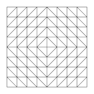
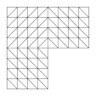
Figure 1: Initial mesh for adaptive method. The unit square (left) with $h=\sqrt{2}/8$ and the L-shaped domain(right) with $h=\sqrt{2}/4$.

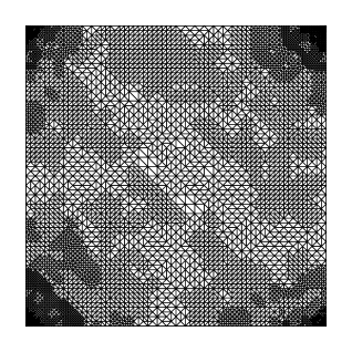
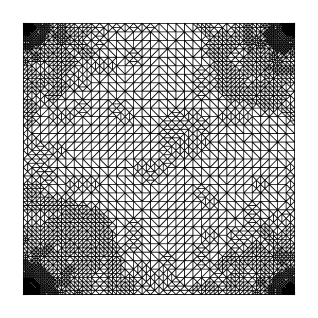
Figure 2: Adaptive meshes for the first eigenvalue on the unit square for Case 1 obtained by the $P_{3}$ element (left) and the $P_{4}$ element (right), respectively.

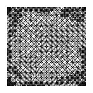
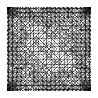
Figure 3: Adaptive meshes for the fifth eigenvalue on the unit square for Case 1 obtained by the $P_{3}$ element (left) and the $P_{4}$ element (right), respectively.

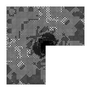
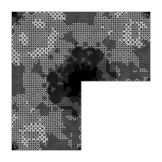
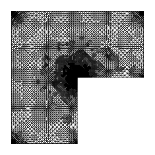
Figure 4: Adaptive meshes for the first eigenvalue on the L-shaped domain for Case 2 obtained by the $P_{1}$ element (top left), the $P_{2}$ element (top right), the $P_{3}$ element (bottom left) and the $P_{4}$ element (bottom right) respectively.

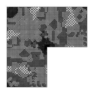
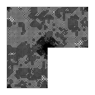
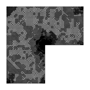
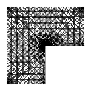
Figure 5: Adaptive meshes for the sixth eigenvalue on the L-shaped domain for Case 2 obtained by the $P_{1}$ element (top left), the $P_{2}$ element (top right), the $P_{3}$ element (bottom left) and the $P_{4}$ element (bottom right) respectively.

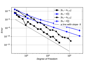
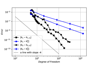
Figure 6: Error curves for the first and fifth eigenvalues on the unit square for Case 1 obtained by the $P_{3}$ element (left) and the $P_{4}$ element (right), respectively.

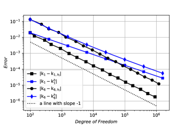
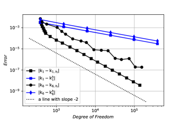
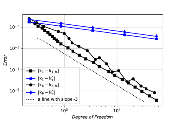
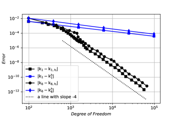
Figure 7: Error curves for the first and sixth eigenvalues on the L-shaped domain for Case 2 obtained by the $P_{1}$ element (top left), the $P_{2}$ element (top right), the $P_{3}$ element (bottom left) and the $P_{4}$ element (bottom right) respectively.

Table 1: The approximate eigenvalues on the unit square for Case 1 obtained by the $P_{4}$ element with the initial uniform mesh $(h_{0}=\sqrt{2}/4)$.

$j$	$l$	${DoF}_{j,l}$	$\mathrm{k}_{j,h_{l}}$	$j$	$l$	${DoF}_{j,l}$	$\mathrm{k}_{j,h_{l}}$
1	0	514	2.678560407762189	5,6	0	514	5.8250906361254$\pm$0.8501997542054$\mathrm{i}$
1	5	834	2.6785663637974375	5,6	5	834	5.8251047037874$\pm$0.8502156894591$\mathrm{i}$
1	10	1218	2.6785666048173606	5,6	10	3106	5.8251046903523$\pm$0.8502179171864$\mathrm{i}$
1	15	4434	2.678566641438936	5,6	13	7314	5.8251046825744$\pm$0.8502179048201$\mathrm{i}$
1	16	5874	2.6785666415793807	5,6	14	9266	5.8251046828306$\pm$0.8502179047199$\mathrm{i}$
1	17	7618	2.678566641653595	5,6	15	12802	5.8251046826660$\pm$0.8502179044386$\mathrm{i}$
1	18	10114	2.678566641668692	5,6	16	15698	5.8251046826741$\pm$0.8502179042839$\mathrm{i}$
1	19	13106	2.6785666416729192	5,6	17	21058	5.8251046826744$\pm$0.8502179042968$\mathrm{i}$
1	20	17778	2.6785666416740033	5,6	18	26882	5.8251046826680$\pm$0.8502179043068$\mathrm{i}$
1	21	23346	2.6785666416746796	5,6	19	31666	5.8251046826673$\pm$0.8502179043080$\mathrm{i}$

Table 2: The approximate eigenvalues on the L-shaped domain for Case 2 obtained by the $P_{4}$ element with the initial uniform mesh $(h_{0}=\sqrt{2}/2)$.

$j$	$l$	${DoF}_{j,l}$	$\mathrm{k}_{j,h_{l}}$	$j$	$l$	${DoF}_{j,l}$	$\mathrm{k}_{j,h_{l}}$
1	0	386	0.8755661700754	6,7	0	386	3.0490526389229$\pm$0.0822453289680 $\mathrm{i}$
1	5	882	0.8741362387888	6,7	5	1314	3.0467668650725$\pm$0.0815300508826 $\mathrm{i}$
1	10	1346	0.8739876304907	6,7	10	3138	3.0448876037668$\pm$0.0824072414907$\mathrm{i}$
1	15	1842	0.8739736924251	6,7	15	11074	3.0448402133483$\pm$0.0824124057516 $\mathrm{i}$
1	20	3586	0.8739708340761	6,7	19	27554	3.0448395440036$\pm$0.0824124707211$\mathrm{i}$
1	25	10818	0.8739706756303	6,7	20	34946	3.0448395438721$\pm$0.0824124707252$\mathrm{i}$
1	28	22242	0.8739706738797	6,7	21	42210	3.0448394615373$\pm$0.0824124783664$\mathrm{i}$
1	29	29410	0.8739706738016	6,7	22	52770	3.0448394615119$\pm$0.0824124783794$\mathrm{i}$
1	30	35762	0.8739706737785	6,7	23	66114	3.0448394614984$\pm$0.0824124783762$\mathrm{i}$
1	31	44978	0.8739706737685	6,7	24	78818	3.0448394512079$\pm$0.0824124793275$\mathrm{i}$

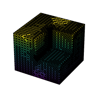
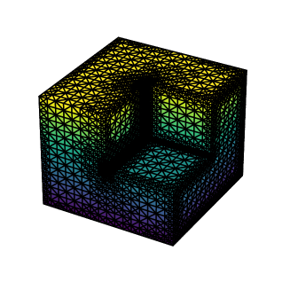
Figure 8: The surfaces of adaptive meshes for the first eigenvalue on the Fichera domain for Case 3 obtained by the $P_{1}$ element (left) and the $P_{2}$ element (right), respectively

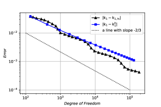
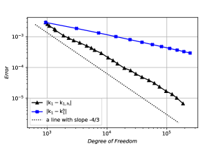
Figure 9: Error curves for the first eigenvalue on the Fichera domain for Case 3 obtained by the $P_{1}$ element (left) and the $P_{2}$ element (right), respectively.

Table 3: The first approximate eigenvalues on the Fichera domain for Case 3 obtained by the $P_{2}$ element with the initial uniform mesh $(h_{0}=\sqrt{3}/2)$.

$l$	${DoF}_{1,l}$	$\mathrm{k}_{1,h_{l}}$	$l$	${DoF}_{1,l}$	$\mathrm{k}_{1,h_{l}}$	$l$	${DoF}_{1,l}$	$\mathrm{k}_{1,h_{l}}$
0	944	1.07062332	9	4580	1.06818946	18	30464	1.06774425
1	1008	1.07028496	10	5484	1.06811391	19	38662	1.06773074
2	1086	1.06995107	11	6218	1.06805111	20	50392	1.06772048
3	1328	1.06946592	12	8026	1.06797512	21	62252	1.06771302
4	1380	1.06930904	13	10446	1.06789139	22	75812	1.06770574
5	1874	1.06877474	14	12652	1.06785206	23	97534	1.06769919
6	2290	1.06859255	15	14980	1.06781498	24	123350	1.06769565
7	2772	1.06844332	16	19566	1.06777787	25	147234	1.06769242
8	3510	1.06832147	17	24912	1.06776204	26	187504	1.06768887

References

• [1] F. Cakoni, M. Cayoren, D. Colton, Transmission eigenvalues and the nondestructive testing of dielectrics, Inverse Problems 24(2008) 065016.
• [2] F. Cakoni, H. Haddar, Transmission eigenvalues in inverse scattering theory, Inverse problems and applications: inside out. II, 529-580. Math. Sci. Res. Inst. Publ., 60, Cambridge Univ. Press, Cambridge, 2013.
• [3] D. Colton, R. Kress, Inverse Acoustic and Electromagnetic Scattering Theory, second ed., in: Applied Mathematical Sciences, vol. 93, Springer, New York, 1998.
• [4] D. Colton, P. Monk, J. Sun, Analytical and computational methods for transmission eigenvalues, Inverse Problems 26 (2010) 045011.
• [5] F. Cakoni, D. Colton, H. Haddar, Inverse Scattering Theory and Transmission Eigenvalues, Philadelphia: SIAM, 2016.
• [6] J. Sun, A. Zhou, Finite Element Methods for Eigenvalue Problems, CRC Press, Taylor Francis Group, Boca Raton, London, New York, 2016.
• [7] J. An, Legendre-Galerkin spectral approximation and estimation of the index of refraction for transmission eigenvalues, Appl. Numer. Math. 108 (2016) 171-184.
• [8] F. Zeng, J. Sun, L. Xu, A spectral projection method for transmission eigenvalues, Sci. China Math. 59 (2016) 1613-1622.
• [9] Y. Yang, H. Bi, H. Li, J. Han, Mixed methods for the Helmholtz transmission eigenvalues, SIAM J. Sci. Comput. 38 (2016) A1383-A1403.
• [10] H. Geng, X. Ji, J. Sun, and L. Xu, $C^{0}$IP methods for the transmission eigenvalue problem, J. Sci. Comput. 68(2016) 326-338.
• [11] H. Chen, H. Guo, Z. Zhang, and Q. Zou, A $C^{0}$ linear finite element method for two fourth-order eigenvalue problems, IMA J. Numer. Anal. 37(2017) 2120-2138.
• [12] T. Li, T.M. Huang, W.W. Lin, and J.N. Wang, An efficient numerical algorithm for computing densely distributed positive interior transmission eigenvalues, Inverse Problems 33(3) (2017) 035009.
• [13] J. Han, Y. Yang, An $H^{m}$-conforming spectral element method on multi-dimensional domain and its application to transmission eigenvalues, Sci. China Math. 60(8)(2017) 1529-1542.
• [14] A. Kleefeld and D. Colton, Interior transmission eigenvalues for anisotropic media. Integral methods in science and engineering. Vol. 1. Theoretical techniques, 139-147, Birkh$\ddot{a}$user/Springer, Cham, 2017.
• [15] A. Kleefeld and L. Pieronek, Computing interior transmission eigenvalues for homogeneous and anisotropic media, Inverse Problems 34(10)(2018) 105007.
• [16] A. Kleefeld and L. Pieronek, The method of fundamental solutions for computing acoustic interior transmission eigenvalues, Inverse Problems 34(3)(2018) 035007.
• [17] J. Cama$\tilde{n}o$, R. Rodr$\acute{i}$guez, and P. Venegas, Convergence of a lowest-order finite element method for the transmission eigenvalue problem, Calcolo 55(3)(2018) Article 33.
• [18] D. Mora and I. Vel$\acute{a}$s quez, A virtual element method for the transmission eigenvalue problem, Math. Models Methods Appl. Sci. 28(14)(2018) 2803-2831.
• [19] H. Li, Y. Yang, An adaptive $C^{0}$IPG method for the Helmholtz transmission eigenvalue problem, Sci. China Math. 61(8)(2018) 1519-1542
• [20] Y. Yang, Y. Zhang, H. Bi, A type of adaptive $C^{0}$ non-conforming finite element method for the Helmholtz transmission eigenvalue problme, Comput. Methods Appl. Mech. Engrg. 360(2020) 112697
• [21] X. Ji, J. Sun, A multi-level method for transmission eigenvalues of anisotropic media, J. Comput. Phys. 255(2013) 422-435.
• [22] H. Xie, X. Wu, A multilevel correction method for interior transimission eigenvalue problem, J. Sci. Comput. 72(2017) 586-604.
• [23] B. Gong, J. Sun, T. Turner and C. Zheng, Finite element approximation of transmission eigenvalues for anisotropic media, preprint (2020), arXiv:2001.05340v1.
• [24] A.S. Bonnet-Ben Dhia, P.J. Ciarlet, C.M. Zw$\ddot{o}$lf, Time harmonic wave diffraction problems in materials with sign-shifting coefficients, J. Comput. Appl. Math. 234(2010) 1912-1919.
• [25] A.S. Bonnet-Ben Dhia, L. Chesnel, H. Haddar, On the use of T-coercivity to study the interior transmission eigenvalue problem, C. R. Acad. Sci. Paris Ser. I 349(2011) 647-651.
• [26] A.S. Bonnet-Ben Dhia, L. Chesnel, P.J. Ciarlet, T-coercivity for scalar interface problems between dielectrics and metamaterials, ESAIM: M2AN 46(2012) 1363-1387.
• [27] L. Chesnel, P.J. Ciarlet, T-coercivity and continuous Galerkin methods: application to transmission problems with sign changing coefficients, Numer. Math. 124(2013) 1-29.
• [28] X. Wu, W. Chen, Error estimates of the finite element method for interior transmission problems, J. Sci. Comput. 57(2)(2013) 331-348.
• [29] P.J. Ciarlet, $T$-coercivity: application to the discretization of Helmholtz-like problems, Comput. Math. Appl. 64(2012) 22-34.
• [30] J. Gedicke, C. Carstensen, A posteriori error estimators for convection-diffusion eigenvalue problems, Comput. Methods Appl. Mech. Engrg. 268(2014) 160-177.
• [31] R. Gasser, J. Gedicke, S. Sauter, Benchmark computation of eigenvalues with large defect for non-self-adjoint elliptic differential operators, SIAM J. Sci. Comput. 41(6) A3938-A3953.
• [32] P. Grisvard, Elliptic Problems in Nonsmooth Domains, Boston: Pitman, 1985.
• [33] M. Ainsworth, J.T. Oden, A posteriori error estimates in the finite element analysis, New York: Wiley-Inter science, 2011.
• [34] I. Babu$\check{s}$ka, W.C. Rheinboldt, Error estimates for adaptive finite element computations, SIAM J. Numer. Anal. 15(1978) 736-754.
• [35] S.C. Brenner, $C^{0}$ interior penalty methods, In Frontiers in Numerical Analysis-Durham 2010, Lecture Notes in Computational Science and Engineering 2012, 85: 79-147, Springer-Verlag.
• [36] P. Morin, R. H. Nochetto, K. Siebert, Convergence of adaptive finite element methods, SIAM Rev. 44(2002) 631-658.
• [37] Z. Shi, M. Wang, Finite Element Methods, Science Press, Beijing, 2013.
• [38] R. Verf$\ddot{u}$rth, A review of a posteriori error estimates and adaptive mesh-refinement techniques, Wiley-Teubner, New York, 1996.
• [39] I. Babu$\check{s}$ka, J.E. Osborn, Eigenvalue problems, in: P.G. Ciarlet, J.L. Lions (Eds.), Finite Element Methods (Part 1) Handbook of Numerical Analysis, Vol. 2, Elsevier Science Publishers, North-Holand, 1991, pp. 640-787.
• [40] D. Boffi, Finite element approximation of eigenvalue problems, Acta Numer. (2010) 1-120.
• [41] S.C. Brenner, L.R. Scott, The Mathematical Theory of Finite Element Methods, second ed., Springer-Verlag, New york, 2002.
• [42] P.G. Ciarlet, Basic error estimates for elliptic proplems, in: P.G. Ciarlet, J.L. Lions (Eds.), Finite Element Methods (Part1) Handbook of Numerical Analysis, Vol. 2, Elsevier Science Publishers, North-Holand, 1991, pp. 17-351.
• [43] J.T. Oden, J.N. Reddy, An Introduction to the Mathematical Theory of Finite Elements, Courier Dover Publications, New York, 2012.
• [44] I. Babu$\check{s}$ka, A. Aziz, Survey lectures on the mathematical foundations of the finite element method, in: A.K. Aziz, ed., The Mathematical Foundations of the Finite Element Method with Application to Partial Differential Equations, Academic Press, New York, 5-359
• [45] Y. Yang, S. Wang, H. Bi, The finite element method for the elastic transmission eigenvalue problme with different elastic tensors, J. Sci. Comput. (2022) 93:65
• [46] L. R. Scott, S. Zhang, Finite element interpolation of non-smooth functions satisfying boundary conditions, Math. Comp. 54(1990) 483-493.
• [47] X. Dai, L. He, A. Zhou, Convergence and quasi-optimal complexity of adaptive finite element computations for multiple eigenvalues, IMA J. Numer. Anal. 35(2014) 1934-1977.
• [48] R. Verf$\ddot{u}$rth, A posteriori error estimators for convection-diffusion equations, Numer. Math. 80(1998) 641-663.
• [49] X. Dai, J. Xu., A. Zhou, Convergence and optimal complexity of adaptive finite element eigenvalue computations, Numer. Math. 110(2008) 313-355.
• [50] W. D$\ddot{o}$rfler, A convergent adaptive algorithm for Poisson’s equation, SIAM J. Numer. Anal. 33(1996) 1106-1124.
• [51] L. Chen, An integrated finite element method package in MATLAB, Technical Report, University of California at Irvine, California, 2009.
• [52] T. Gustafsson, G.D. McBain, scikit-fem: A Python package for finite element assembly, J. Open Source Softw. 5(52)(2020) 2369.