Boosted top tagging and its interpretation using Shapley values

Abstract

Top tagging has emerged to be a fast-evolving subject due to the top quark’s significant role in probing physics beyond the standard model. For the reconstruction of top jets, machine learning models have shown a significant improvement in the tagging and classification performance compared to the previous methods. In this work, we build top taggers using $N$-Subjettiness ratios and several observables of the Energy Correlation functions as input features to train the eXtreme Gradient BOOSTed decision tree (XGBOOST). It is observed that the performance of the taggers depends on how well the top jets are matched to their truth-level partons. Furthermore, we use SHapley Additive exPlanation (SHAP) framework to calculate the feature importance of the trained models. It helps us to estimate how much each feature of the data contributed to the model’s prediction and what regions are of more importance for each input variable. Finally, we combine all the tagger variables to form a hybrid tagger and interpret the results using the Shapley values.

1 Introduction

The Standard Model (SM) top quark is an important probe of new physics. Models of beyond the SM physics (BSM) trying to alleviate the hierarchy problem tHooft:1979rat , like the supersymmetric extensions of the SM Gildener:1976ih ; Susskind:1978ms or the little Higgs models Arkani-Hamed:2001nha ; Arkani-Hamed:2002ikv , include top partners which naturally decay to top quarks. To dig out any new physics from top quarks, we require ways to correctly identify and fully reconstruct them at collider experiments, like the Large Hadron Collider (LHC) experiments. While its leptonic and semi-leptonic decay modes are less challenging to identify in the busy environment of LHC detectors, they lose the scope for full reconstruction owing to the invisible neutrinos in the final state. The hadronic decay mode of top quarks can be fully reconstructed. However, the high jet multiplicity in the final state makes combinatorics challenging. This problem is resolved when we are in the regime of boosted top quarks, where they have very high momenta, which makes their decay products collimated. In the collider detectors, this is then reconstructed as a single object $-$ a fat jet consisting of all the decay products of the top quark.

Traditionally, people applied the algorithms of finding jet substructure to tag top quark jets from a background of jets associated with light quarks or gluons. From taggers based on explicitly reconstructing the subjets inside the fat jet, like John Hopkins Kaplan:2008ie and HepTopTagger  Plehn:2009rk ; Plehn:2010st ; Plehn:2011sj , to using variables that naturally capture the correct pronged structure of a top jet, like $N$-subjettiness Thaler:2010tr , and energy correlation functions Larkoski:2013eya ; Moult:2016cvt , to employing machine learning (ML) techniques like image recognition on jet images with a convolutional neural network (CNN), and networks based on low-level information of a jet across the full detector or high-level variables constructed out of them, top taggers have evolved a lot over the years. There’s a plethora of research works going on in this direction to improve the tagging efficiencies of top quarks Almeida:2015jua ; Kasieczka:2017nvn ; Butter:2017cot ; Macaluso:2018tck ; Moore:2018lsr ; Kasieczka:2019dbj ; Roy:2019jae ; Diefenbacher:2019ezd ; Chakraborty:2020yfc ; Bhattacharya:2020aid ; Lim:2020igi ; Dreyer:2020brq ; Aguilar-Saavedra:2021rjk ; Andrews:2021ejw ; Dreyer:2022yom ; Ahmed:2022hct ; Munoz:2022gjq in experiments to better our chances of observing hints of new physics. Both the ATLAS and CMS experimental collaborations have also included many such sophisticated taggers in their searches which has improved their limits ATLAS:2020lks ; ATL-PHYS-PUB-2020-017 ; ATL-PHYS-PUB-2022-039 ; CMS:2012bti ; CMS:2017ucf ; CMS:2021beq . Since ML algorithms can sometimes be black boxes, it is essential to understand the physics behind what it has learnt and how it can distinguish top jets from others. Several studies, therefore, make attempts to explore the interpretability of these algorithms and their results Grojean:2020ech ; Bradshaw:2022qev ; Khot:2022aky ; Das:2022cjl .

Although being very well-explored, there are still some subtleties that can affect the performance of top tagging algorithms. Most of the ML-based studies on top tagging work with a subset of jets where the decay products of the top quark at the parton level fall within a certain distance from the axis of the fat jet. This ensures that the reconstructed jet contains the full decay of the top quark and is called the “matching” condition Kasieczka:2017nvn ; Macaluso:2018tck ; Kasieczka:2019dbj . The choice of this distance from the jet axis used for matching is somewhat ad hoc, and more importantly, this criterion cannot be used in experiments. This leads us to question the impact of this matching condition on the performance of the various taggers. Moreover, tagging efficiencies depend on the momentum of the initial top quark Kaplan:2008ie , which is again difficult to control in experiments where we only have the momentum of the reconstructed fat jet. A large angle final-state radiation (FSR) or the presence of neutrinos and muons from the decay of $B$ mesons might reduce the energy of the final jet with respect to the initially produced top quark. It is interesting to explore how the migration along different energy bins of the jet reconstructed at the detector compared to the parton-level top quark affects the performance of the various top taggers.

We begin our present study addressing these questions by training XGBOOST DBLP:journals/corr/ChenG16 networks, which is an ML algorithm using the gradient boosting framework. We use various sets of $N$-subjettiness variables and energy correlation functions as inputs to the XGBOOST networks to find out which set of variables among them have better performance as top taggers. Usually, these variables are used to develop cut-based taggers. However, there can be important correlations between them, differentiating the top jets from QCD jets. This motivates their use as inputs to a decision-tree based ML tagger for better identification of such correlations. Furthermore, we train our XGBOOST tagger using the full combination of the $N$-subjettiness variables and Energy Correlation Functions and study the impact of reducing these input variables for the training on the performance of the tagger. Finally, we present an interpretation of our results from the XGBOOST training, making use of the SHAP (SHapley Additive exPlanations) DBLP:journals/corr/LundbergL17 ; DBLP:journals/corr/abs-1802-03888 ; DBLP:journals/corr/abs-1905-04610 ; Shapley+2016+307+318 framework, which is based on Shapley values, defined in the later part of this work. SHAP has been widely used to interpret machine learning output in collider studies Cornell:2021gut ; Alvestad:2021sje ; Grojean:2020ech ; CMS:2021qzz ; Grojean:2022mef ; Adhikary:2022jfp .

The rest of the paper is organized as follows - in Section 2, we discuss the simulation, matching criterion, and the energy bin of the data set of top jets used in this work. In Section 3, we first present a brief review of the $N$-subjettiness variables and the energy correlation functions used for top tagging and then present results of our XGBOOST tagger for each of these sets. In Section 4, we introduce the SHAP framework of interpreting results from the XGBOOST-based taggers, construct a hybrid tagger using variables across the different sets of standard top tagging variables, and interpret the results from this hybrid tagger. We finally conclude in Section 5.

2 Data set of top jets

In this section, we discuss the data set of jets associated with top quarks used by us in the present work. We first briefly outline our simulation details and then describe the matching of the parton-level information to the final reconstructed top jet. This includes ensuring whether the top jet consists of the full hadronic activity of the three partons coming from its decay and whether the energy of the top jet lies in the same bin as the initially generated top quark.

2.1 Simulation details

We generate single top jets using the following process

$$pp\rightarrow tW,\ ~{}~{}t\to bW.$$

The $W$-boson coming from the top quark decay is allowed to decay hadronically only, while the other $W$-boson decays leptonically (we choose a muonic mode only). Gluon-initiated jets are also analyzed to estimate the mistagging rates. We simulate the QCD-jets using the following process

$$pp\rightarrow Zg$$

with $Z$ decaying invisibly.

We put a generation level cut on $p_{T,t}$ (signal) or $p_{T,g}$ (background) of 450 GeV. The hard collision events are generated using MadGraph (MG5_aMC_v2_8_2) Alwall:2011uj ; Alwall:2014hca , and then passed to PYTHIA 8 Sjostrand:2007gs for hadronization and parton shower. Jets are generated with initial-state radiation (ISR), final-state radiation (FSR), and multiple parton interaction (MPI) effects. Delphes-3.5.0 deFavereau:2013fsa is used to simulate detector effects where we use the default ATLAS card. We use the cteq6l1 PDF set from LHAPDF6 Buckley:2014ana along with the ATLAS UE Tune AU2-CTEQ6L1 for the event generation. The simulated events are reconstructed to jets using Cambridge-Aachen (C/A) jet clustering algorithm Dokshitzer:1997in and a fixed jet radius parameter R = 1.0. We change the segmentation of the Hadronic Calorimeter (HCAL) to $\sim 0.1\times 0.1$ in $\eta-\phi$ plane with $|\eta|$ extended up to 3.0. Jets are clustered using the calorimeter tower elements. We consider the leading jet with $p_{T}=[500,600)$ GeV, and $|\eta|<2.5$, and store its constituents to construct different observables, which are then used as inputs to the various top taggers, as discussed in the next section.

2.2 Matching of the partons with the top jet

The top ($t$) quark decays to a $b$ quark and a $W$ boson, and the $W$ further decays to two light quarks, which we shall refer to from now on as $u$ and $d$. Thus, the final state contains three quarks. In the left (right) panel of Figure 1, we plot the 2-D distribution of the fraction of the top’s $p_{T}$ carried away by a b (u) quark and the distance of the b (u) quark from t in $\eta-\phi$ plane. The distance between two objects in the $\eta-\phi$ plane is given by $\Delta R=\sqrt{(\Delta\eta_{ij})^{2}+(\Delta\phi_{ij})^{2}}$. We see that the softer the parton is, the farther it is from t. Since u and d decay from a W, they are softer than b and have a wider spread in $p_{T}$ as can be seen in Figure 1.

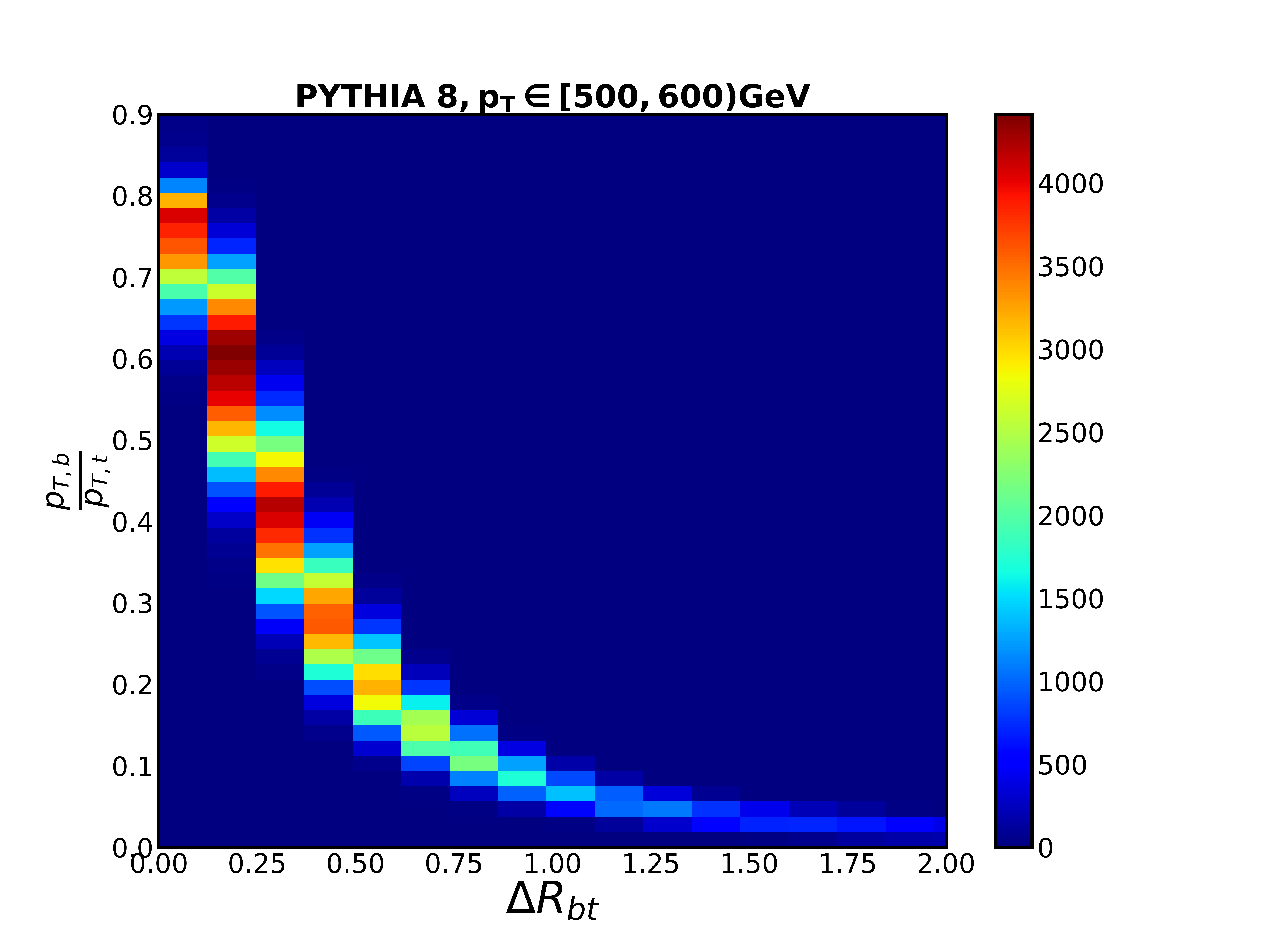
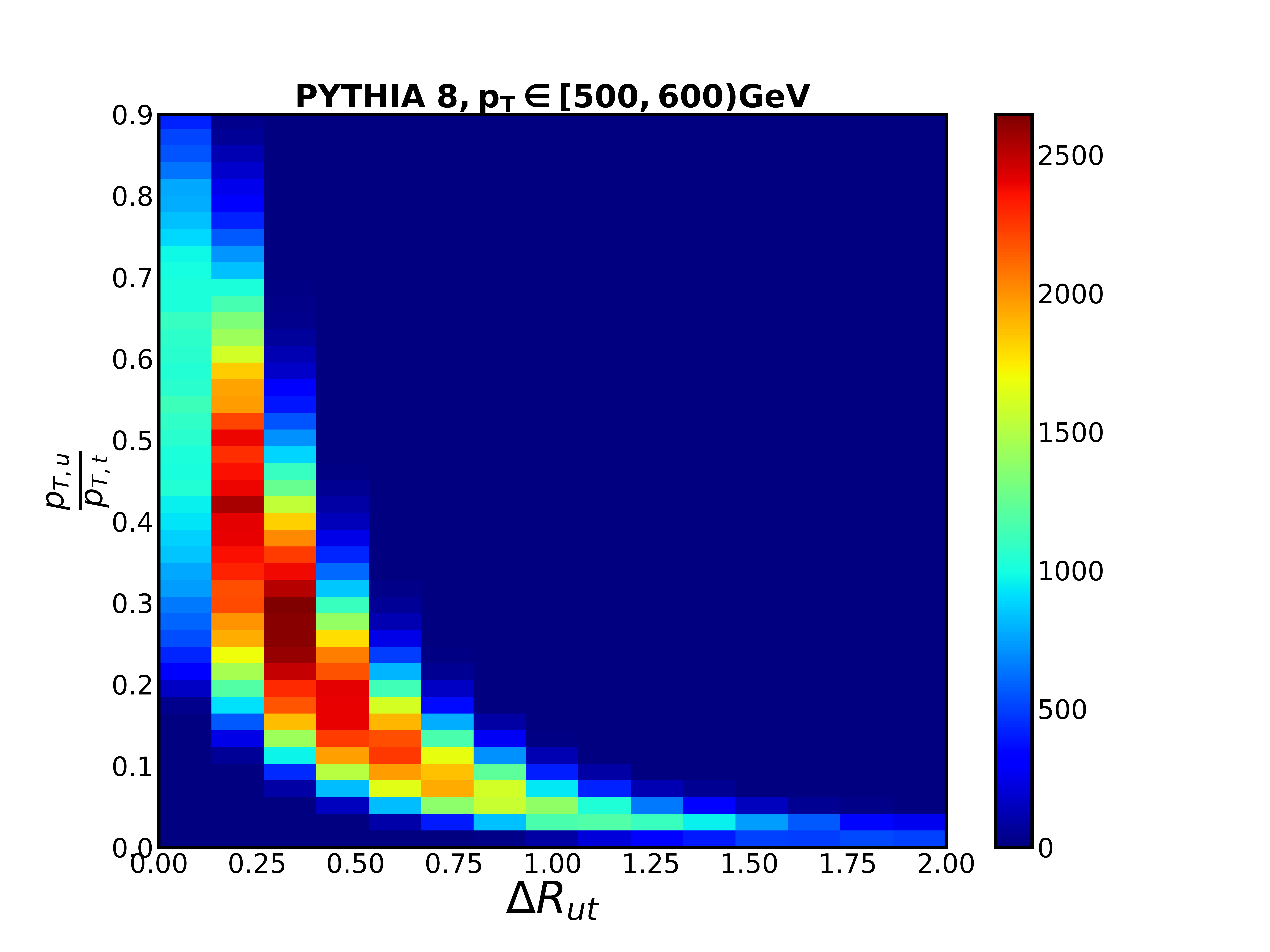
Figure 1: Left: 2-D histogram of $p_{T}$ fraction carried by a b parton and the $\Delta R$ between b and t at the truth level. Right: 2-D histogram of $p_{T}$ fraction carried by a u parton and the $\Delta R$ between u and t at the truth level, where u represents one of the decay products of W. The colour bar shows the density of a bin.

It is a common practice to process top jets before using them to train any machine learning (ML) classifier by selecting only those top jets which contain the initial partons b,u and d matched within a radius $\Delta R_{m}$ from the jet axis. The matching radius $\Delta R_{m}$ is typically the same as the jet radius. We select three matching radii for our analysis, $\Delta R_{m}$ = 0.6, 0.8, 1.0. We also consider top jets without being subjected to any matching procedure, which we shall refer to as unmatched criteria from now on. Table 1 shows the fraction of top jets belonging to each category and the fraction of top jets where one quark lies outside $\Delta R_{m}$. All jets have $p_{T}\in[500,600)$ GeV. The last row corresponds to the unmatched samples.

$p_{T}^{J}\in[500,600)$ GeV
Matching radius $\Delta R_{m}$	Fraction of top jets fulfilling matching criteria	Fraction of top jets where one quark lies outside $\Delta R_{m}$
0.6	0.3	0.6
0.8	0.6	0.4
1.0	0.7	0.3
unmatched	1.0	NA

Table 1: Fraction of top jets that pass the matching criteria with four different matching criteria $\Delta R_{m}$ = 0.6, 0.8, 1.0 and unmatched and the fraction of top jets where one parton fails the matching criteria.

Before going into the taggers themselves, we consider the jet mass variable $m_{jet}$ for the different categories of top jets. Figure 2 shows the normalized $m_{jet}$ distribution for four cases of $\Delta R_{m}$ and gluon jets. As our matching criteria tightens, we see that the jet mass variable reconstructs the top quark mass more accurately. For unmatched jets, i.e., when no matching criteria is applied, the $m_{jet}$ distribution becomes flatter, and a peak forms at W mass, populated by events where one of the quarks lies outside the jet cone radius.

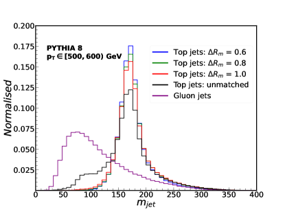
Figure 2: Normalised $m_{jet}$ distribution of top jets with $\Delta R_{m}$ = 0.6, 0.8, 1.0, unmatched top jets, and gluon jets.

As mentioned, we generate truth-level events by applying a cut on $p_{T}$ > 450 GeV because we primarily study jets with $p_{T}\in[500,600)$ GeV for our analysis. There remains the possibility of a top quark having an initial $p_{T}$ > 600 GeV, which then loses energy and migrates to the $p_{T}\in[500,600)$ bin. To see this effect into play, we generate signal events with a generation level cut of $p_{T,t}$ > 600 GeV and then select those jets which lie in the $p_{T}\in[500,600)$ bin. Figure 3 shows the correlation between $p_{T}$ of the top quark and of the final top jet for the two $p_{T}$ cuts at the generation level. From the left panel, we see that while most events carry their initial energy from parton to jets, there are also events that undergo bin migration. The right panel shows that such events that migrate from higher to lower $p_{T}$ mainly populate the upper half of the $p_{T}\in[500,600)$ GeV bin, as expected.

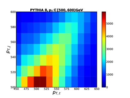
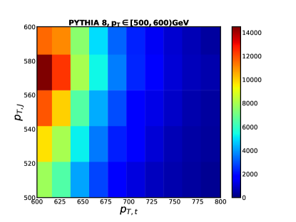
Figure 3: 2-D histogram of truth level top quark $p_{T}$ and selection level top jet $p_{T}$ when generation $p_{T}$ cut is 450 GeV (left) and 600 GeV (right). The colour bar shows the number of points in a bin.

The phenomenon of bin migration affects variables like jet mass. Figure 4 shows the $m_{jet}$ distribution of unmatched jets. Jets that lose energy to have $p_{T}\in[500,600)$ GeV have lower $m_{jet}$ values, resulting in their distribution to shift towards lower $m_{jet}$.

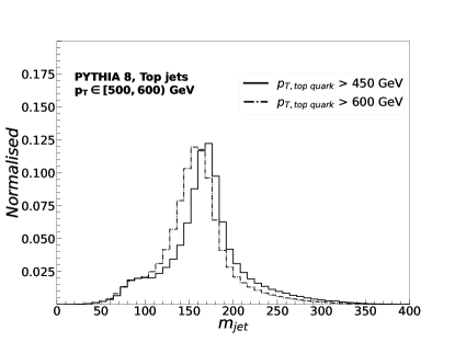
Figure 4: Normalised $m_{jet}$ distribution of top jets for unmatched top jets with the two different generation level $p_{T}$ cuts.

3 Standard top taggers and XGBOOST

In this section, we briefly review the observables used in the standard top taggers, namely $N$-subjettiness Thaler:2010tr and Energy Correlation Functions Larkoski:2013eya and their ratios. We use the fastjet-contrib library, which is an extension of Fastjet Cacciari:2005hq ; Cacciari:2011ma package, to construct these tagger variables. These variables are well documented in existing literature where their proficiency in top tagging has been extensively studied and implemented. Prior works have also discussed advanced top taggers where machine learning techniques have given better performance with a combination of such high-level variables as well as jet images and four momentum of jet constituents Almeida:2015jua ; Kasieczka:2017nvn ; Butter:2017cot ; Moore:2018lsr ; Macaluso:2018tck ; Kasieczka:2019dbj ; Roy:2019jae ; Diefenbacher:2019ezd ; Chakraborty:2020yfc ; Bhattacharya:2020aid ; Lim:2020igi ; Dreyer:2020brq ; Aguilar-Saavedra:2021rjk ; Andrews:2021ejw ; Dreyer:2022yom ; Ahmed:2022hct ; Munoz:2022gjq . Any machine learning-based top-tagger that uses kinematic variables has the basic underlying strategy: it takes the variables as input or features for each event, trains on many such events, and produces a probability score for each event in the test data set. For a binary classification, the output can be either a higher probability score of the event being a top jet or a lower probability, meaning it is a QCD jet.

Our work uses a decision tree-based algorithm: the eXtreme Gradient BOOSTed decision tree DBLP:journals/corr/ChenG16 . XGBOOST implements gradient-boosted decision trees designed for speed and performance. The model is trained on top and gluon jets generated with the four categories of truth level matching process used earlier. Each category has 600k top jets and 600k gluon jets for training, 200k top jets and 200k gluon jets for validation, and 200k top jets and 200k gluon jets for testing. Details of generation and simulation are listed in Section 2.1.

The decision tree uses binary:logloss as the objective loss function with a learning rate of 0.1 and maximum depth set to 5. To prevent overfitting, we use early stopping, which tells the model to stop training if validation performance continues to degrade after 5 rounds. The Area Under the Curve (AUC) metric evaluates the performance of the trained model. The input features are divided into sets: $N$-Subjettiness, C-series, D-series, M-Series, N-Series, and U-series. Each set also includes the jet mass variable: $m_{jet}$. We also construct these variables on pruned jets. Pruning Ellis:2009me is a technique by which soft particles are removed from a jet if the following conditions hold while recombining two particles $i$ and $j$:

$$\frac{min(p_{T}^{i},p_{T}^{j})}{p_{T}^{i+j}}<z_{cut}~{}and~{}\Delta R_{ij}>r_{cut}$$ (1)

If the above condition is satisfied, the softer particle is discarded, and the jet algorithm reconstructs a pruned jet. We set the two parameters $z_{cut}$ and $r_{cut}$ to be 0.1 and 0.5, respectively.

In the following section, we describe the variables used and also present the test accuracy and AUC of a trained XGBOOST model for jets matched with $R_{m}$ = 0.6, 0.8, 1.0, and unmatched jets, using as input features, variables constructed on unpruned jets, pruned jets and both combined. The test accuracy is the percentage of correctly identified tops and gluons in the test dataset based on a threshold probability score of 0.5.

3.1 $N$-Subjettines

$N$-Subjettiness Thaler:2010tr is a variable to count subjets inside a fat jet. It is defined as

$$\tau_{N}^{(\beta)}=\frac{1}{\sum_{\alpha\in\text{jet}}p_{T,\alpha}R_{0}^{\beta}}\sum_{\alpha\in\text{jet}}p_{T,\alpha}\min_{k=1,...,N}(\Delta R_{k,\alpha})^{\beta}$$ (2)

relative to $N$ subjet directions $\hat{n}_{j}$ and where $\beta>0$ is an arbitrary weighting exponent to ensure infrared safety. For any $N$-prong jet, the ratio $\tau_{N}/\tau_{N-1}$ is expected to drop. Therefore, for top decays producing three separated subjets, the ratio $\tau_{3}/\tau_{2}$ is expected to peak at lower values, compared to the QCD case. Typically, a jet is tagged as a top if the jet mass ($m_{jet}$) falls within a specific window of the actual top mass $m_{t}$ and the ratio $\tau_{32}^{(\beta)}=\tau_{3}^{(\beta)}/\tau_{2}^{(\beta)}$ is smaller than some particular value. However, other $N$-Subjettiness ratios like $\tau_{21}^{(\beta)}=\tau_{2}^{(\beta)}/\tau_{1}^{(\beta)}$ might also have some distinguishing power between the top and QCD jets.

Figure 5 shows the $\tau_{32}^{(1.0)}$ distribution for top jets matched with different $\Delta R_{m}$, and for gluon jets. Smaller $\Delta R_{m}$ shifts the $\tau_{32}^{(\beta)}$ to lower values by making the jets more three-prong-like. From Figure 1, we know that the $\Delta R$ between the top and its decay products is inversely proportional to the $p_{T}$ of the latter. By tightening $\Delta R_{m}$, it is also ensured that the jet constituents along the prongs have higher $p_{T}$.

From the truth level information of top jets, we compute $p_{T}$ fractions of partons ($p_{T,p}/p_{T,t},~{}p=~{}b,~{}u,~{}d)$ and select the minimum, $f_{p_{T}}^{min}=\min(\frac{p_{T,b}}{p_{T,t}},\frac{p_{T,u}}{p_{T,t}},\frac{p_{T,d}}{p_{T,t}})$. $f_{p_{T}}^{min}$ thus refers to the softest $p_{T}$ fraction carried by a top decay product. It turns out that lower values of $f_{p_{T}}^{min}$ yield higher $\tau_{32}^{(1.0)}$, as can be seen in Figure 5 (right). When the softest parton out of the three is too soft, the jet loses its three-prong structure; hence $\tau_{32}$ acquires a higher value.

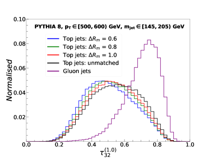
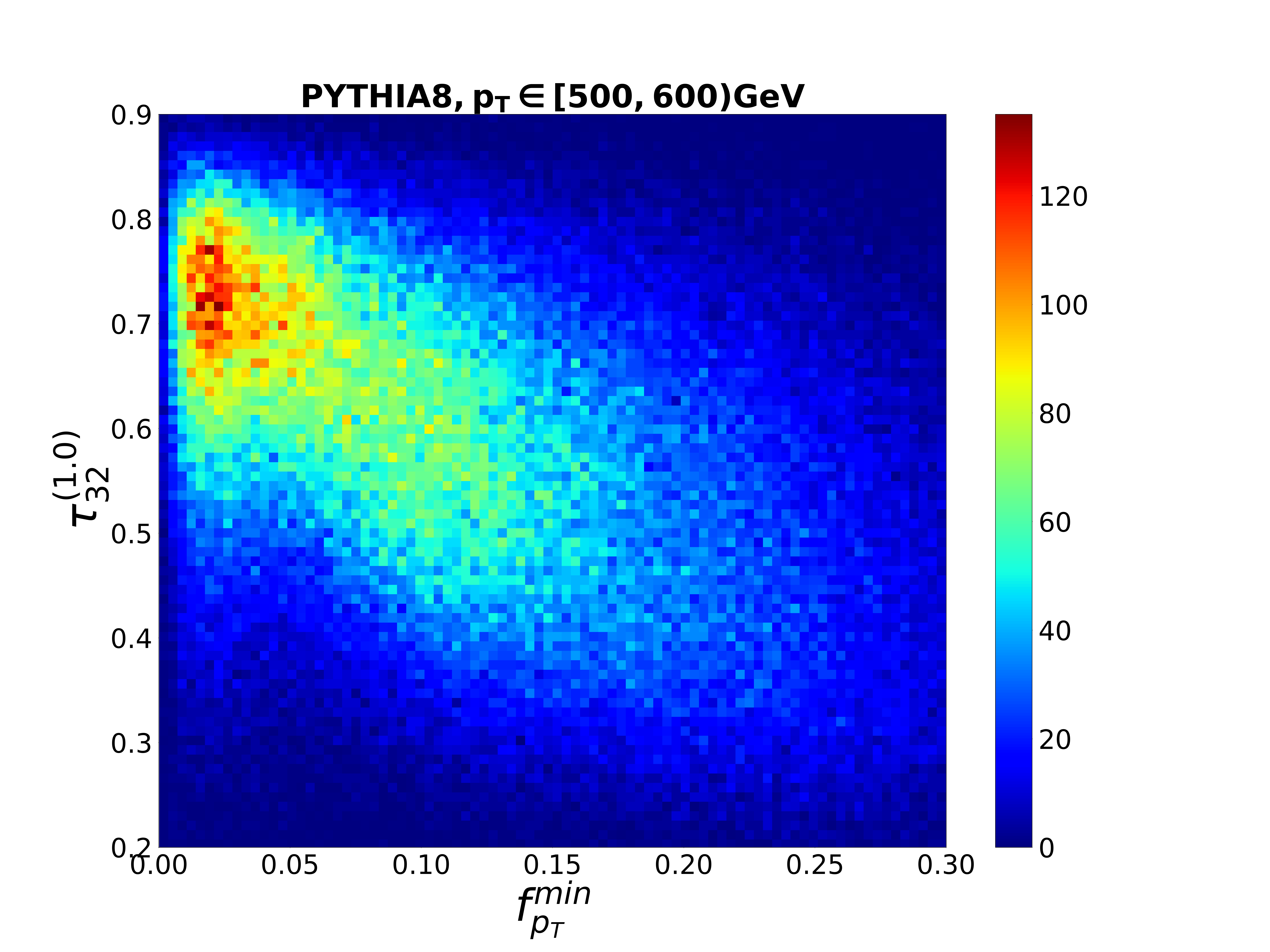
Figure 5: Left: Normalised $\tau_{32}^{(1.0)}$ distribution of top and gluon jets for $\Delta R_{m}$ = 0.6, 0.8, 1.0, and $\infty$, and gluon jets. Right: 2-D distribution of $f_{p_{T}}^{min}$ and $\tau_{32}^{(1.0)}$ for unmatched top jets. Colorbar shows the density in each bin.

We combine the following $N$-Subjettiness variables as inputs to our XGBOOST model.

$$\tau_{21}^{(\beta)},~{}\tau_{32}^{(\beta)},~{}\tau_{43}^{(\beta)},~{}\tau_{54}^{(\beta)},~{}\tau_{65}^{(\beta)}(\beta=0.5,1.0,2.0),~{}and~{}m_{jet}$$ (3)

Table 2 shows the test accuracy and AUC for unpruned, pruned, and combined cases. The results depend on the matching radius $\Delta R_{m}$. Both test accuracy and AUC decrease with an increase in $\Delta R_{m}$. This can be understood from the distribution of $\tau_{32}^{(1.0)}$ in Figure 5, which shows more separation between the top and gluon jets with smaller matching radii. The set with pruned $N$-Subjettiness ratios perform worse than the unpruned case, and combining both improves the performance of the unpruned tagger only slightly.

$p_{T}^{J}\in[500,600)$ GeV
Matching radius $\Delta R_{m}$	$m_{jet}$, $N$-Subjettiness: $\tau_{21}^{(\beta)},~{}\tau_{32}^{(\beta)},~{}\tau_{43}^{(\beta)},~{}\tau_{54}^{(\beta)},~{}\tau_{65}^{(\beta)}$ ($\beta$ = 0.5, 1.0, 2.0)
	unpruned		pruned: $z_{cut}=0.1,~{}D_{cut}=0.5$		pruned & unpruned
	Test Accuracy	AUC	Test Accuracy	AUC	Test Accuracy	AUC
0.6	0.923	0.978	0.896	0.962	0.925	0.978
0.8	0.910	0.971	0.879	0.950	0.913	0.972
1.0	0.898	0.964	0.868	0.941	0.901	0.965
unmatched	0.849	0.926	0.824	0.901	0.852	0.928

Table 2: Test accuracy and AUC of XGBOOST trained with $m_{jet}$ and $N$-Subjettiness ratios in the unpruned, pruned, and combined scenario. The rows refer to the different matching criteria for top jets used to train and test the model.

3.2 Energy Correlation Functions

The normalized $n$-point Energy Correlation Function (ECF) is defined in Larkoski:2013eya as,

$$e_{n}^{(\beta)}=\frac{1}{p_{T,J}^{n}}\sum_{i_{1}<i_{2}<...<i_{n}\in J}(\prod_{a=1}^{n}p_{T,i_{a}})(\prod_{b=1}^{n-1}\prod_{c=b+1}^{n}R_{i_{b}i_{c}})^{\beta}$$ (4)

J denotes a jet, and $p_{T,J}$ is the transverse momenta of that jet. The sum runs over all the particles in J with $R_{ij}^{2}=(\phi_{i}-\phi_{j})^{2}+(y_{i}-y_{j})^{2}$ where $\phi$ and $y$ are the azimuthal angle and rapidity of a particle respectively. The first term in brackets is just the product of the transverse momenta of n particles. The second term is the product of separation variables between $\binom{n}{2}$ pairs of particles out of the n particles. The angular exponent $\beta$ is a free parameter, we set $\beta$ > 0 to make it infrared and collinear safe. From the definition, it is clear that an $n$-pronged jet will yield a smaller value of $e_{n+1}^{\beta}$ compared to $e_{n}^{\beta}$. It has been shown that ratios constructed out of these functions by power counting analysis Larkoski:2013eya ; Larkoski:2014gra ; Moult:2016cvt provide good discrimination between top and QCD jets.

In the following sections, we list 5 series of variables formulated using ECFs and combine some of these variables from each series to build a top tagger. In each section, we list the performance of 5 such top taggers on our test data sets while using unpruned, pruned, and combined sets of variables.

3.2.1 The C-Series

The $C_{i}$ series is defined in Larkoski:2013eya as:

$$C_{i}^{(\beta)}=\frac{e_{n+1}^{(\beta)}e_{n-1}^{(\beta)}}{(e_{n}^{(\beta)})^{2}}$$ (5)

According to Ref. Larkoski:2013eya , $C_{3}^{(\beta)}$ along with a mass cut has considerable discriminating power for 3-prong jets.

$$C_{3}^{(\beta)}=\frac{e_{4}^{(\beta)}e_{2}^{(\beta)}}{(e_{3}^{(\beta)})^{2}}$$ (6)

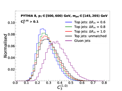
Figure 6: Normalised $C_{3}^{(1.0)}$ distribution of top and gluon jets for $\Delta R_{m}$ = 0.6, 0.8, 1.0, and $\infty$, and gluon jets.

To make $C_{3}$ IRC-safe, a cut is applied to $C_{2}$: $C_{2}^{(\beta)}>0.1$ Larkoski:2013eya . Figure 6 shows the distribution of $C_{3}^{(1.0)}$ for top and gluon jets, with respect to the different matching criteria. Although $C_{3}$ is typically used in boosted top tagging, an ML model might capture more correlations from $C_{1}$ and $C_{2}$ variables with different values of $\beta$. The variables from the C-Series used in the XGBOOST analysis are listed below in 7 and the results on the test dataset are listed in Table 3.

$$C_{1}^{(\beta)},C_{2}^{(\beta)},~{}C_{3}^{(\beta)}(\beta=1.0,2.0),~{}and~{}m_{jet}$$ (7)

The unpruned set shows worse performance compared to the $N$-Subjettiness ratios; however, in the case of pruned jets, the C-Series tagger performs better.

$p_{T}^{J}\in[500,600)$ GeV
Matching radius $\Delta R_{m}$	$m_{jet}$, C-Series: $~{}C_{1}^{(\beta)},C_{2}^{(\beta)},~{}C_{3}^{(\beta)}$ ($\beta$ = 1.0, 2.0)
	unpruned		pruned: $z_{cut}=0.1,~{}r_{cut}=0.5$		pruned & unpruned
	Test Accuracy	AUC	Test Accuracy	AUC	Test Accuracy	AUC
0.6	0.917	0.974	0.902	0.966	0.926	0.979
0.8	0.902	0.965	0.885	0.955	0.911	0.971
1.0	0.889	0.956	0.873	0.947	0.898	0.963
unmatched	0.837	0.914	0.829	0.907	0.848	0.924

Table 3: Test accuracy and AUC of XGBOOST trained with $m_{jet}$ and ratios from the C-Series, in the unpruned, pruned, and combined scenario. The rows refer to the different matching criteria for top jets used to train and test the model.

3.2.2 The D-Series

The $D_{3}^{(\alpha,\beta,\gamma)}$ variable defined in terms of the ratios of the ECFs shows a significant discriminating power between three-prong and one/two-prong phase space Larkoski:2014zma . It is defined as,

$$D_{3}^{(\alpha,\beta,\gamma)}=\frac{e_{4}^{(\gamma)}(e_{2}^{(\alpha)})^{\frac{3\gamma}{\alpha}}}{e_{3}^{(\beta)})^{\frac{3\gamma}{\beta}}}+x\frac{e_{4}^{(\gamma)}(e_{2}^{(\alpha)})^{\frac{2\gamma}{\beta}-1}}{e_{3}^{(\beta)})^{\frac{2\gamma}{\beta}}}+y\frac{e_{4}^{(\gamma)}(e_{2}^{(\alpha)})^{\frac{2\beta}{\gamma}-\frac{\gamma}{\alpha}}}{e_{3}^{(\beta)})^{2}},$$ (8)

where x, y are constants whose value depends on top jet kinematics. The above expression is the linear combination of three phase space regions that contain triple splitting, strongly ordered splitting, and soft emissions. Following Larkoski:2014zma , one can define two quantities x and y using the method of power counting which are given below,

$$x=\kappa_{1}\left(\frac{(p_{T}^{cut})^{2}}{m_{top}^{2}}\right)^{\frac{\alpha\gamma}{\beta}-\frac{\alpha}{2}}$$ (9)

$$y=\kappa_{2}\left(\frac{(p_{T}^{cut})^{2}}{m_{top}^{2}}\right)^{\frac{5\gamma}{2}-2\beta}.$$ (10)

We use the following values of the constants, as suggested in Larkoski:2014zma : $\alpha=2,\beta=0.8,\gamma=0.6$, $x=5,y=0.35$, and the scaling parameters $\kappa_{1}=\kappa_{2}=1$. The reason for choosing $\alpha=2$ is because a cut on the jet mass restricts the study to a certain region of the phase space, as given below,

$$e_{2}^{(2)}\sim\frac{m_{J}^{2}}{p_{TJ}^{2}}$$ (11)

In other words, a mass cut is typically applied on the jet, to restrict $e_{2}$ and simplify the phase space with only $e_{3}^{(\beta)}$ and $e_{4}^{(\gamma)}$ remaining. Figure 7 shows the distribution of $D_{3}$ for top jets and gluon jets. We label the three terms of $D_{3}^{(\alpha,\beta,\gamma)}$ without the x and y coefficients as term 1, term 2, and term 3. We use all the terms along with the standard $D_{3}$ variable as input to XGBOOST. We also consider the two-prong discriminant $D_{2}^{(\alpha,\beta)}$ Larkoski:2014gra ; Larkoski:2015kga defined as,

$$D_{2}^{(\alpha,\beta)}=\frac{e_{3}^{(\alpha)}}{(e_{2}^{(\beta)})^{\frac{3\alpha}{\beta}}}$$ (12)

Figure 7 shows the distribution of the full $D_{3}$ variable. Like $\tau_{32}^{(1.0)}$ and $C_{3}^{(1.0)}$, $D_{3}^{(2,0.8,0.6)}$ peaks at lower values for top jets, a property that distinguishes them from QCD background. The variables used in this series are listed below.

$$D_{2}^{(1.0,1.0)},D_{2}^{(1.0,2.0)},D_{2}^{(2.0,1.0)},D_{2}^{(2.0,2.0)},$$ (13)

$$D_{3}:~{}term~{}1,~{}D_{3}:~{}term~{}2,~{}D_{3}:~{}term~{}3,~{}D_{3}^{(2,0.8,0.6)}$$

Table 4 lists the performance of the D-Series tagger. Again, no significant improvement in the performance of the tagger is observed, even after combining the pruned and unpruned data sets.

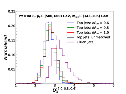
Figure 7: Normalised $D_{3}^{(2.0,0.8,0.6)}$ distribution of top jets for $\Delta R_{m}$ = 0.6, 0.8, 1.0, unmatched top jets, and gluon jets.

$p_{T}^{J}\in[500,600)$ GeV
Matching radius $\Delta R_{m}$	$m_{jet}$, D-Series: $~{}D_{2}^{(\alpha,\beta)}$ ($\alpha$ = 1.0, 2.0, $~{}\beta$ = 1.0, 2.0), $D_{3}:~{}term~{}1,~{}D_{3}:~{}term~{}2,~{}D_{3}:~{}term~{}3,~{}D_{3}^{(2,0.8,0.6)}$
	unpruned		pruned: $z_{cut}=0.1,~{}r_{cut}=0.5$		pruned & unpruned
	Test Accuracy	AUC	Test Accuracy	AUC	Test Accuracy	AUC
0.6	0.922	0.976	0.902	0.965	0.925	0.978
0.8	0.906	0.968	0.884	0.953	0.911	0.970
1.0	0.893	0.960	0.872	0.946	0.898	0.962
unmatched	0.843	0.919	0.828	0.906	0.848	0.925

Table 4: Test accuracy and AUC of XGBOOST trained with $m_{jet}$ and ratios from the D-Series, in the unpruned, pruned, and combined scenario. The rows refer to the different matching criteria for top jets used to train and test the model.

3.2.3 The U-Series

One can also define the generalized correlator functions by replacing the angular part by v factors out of the $\binom{N}{2}$ pairs of angles Moult:2016cvt ,

$${}_{v}e_{n}^{(\beta)}=\sum_{i_{1}<i_{2}<...<i_{N}\in J}z_{i_{1}}z_{i_{2}}..z_{i_{N}}\prod_{m=1}^{v}\min^{(m)}_{s<t\in\{i_{1},i_{2}..i_{N}\}}\left\{\theta^{(\beta)}_{st}\right\}$$ (14)

where

$$z\equiv\frac{p_{T,i}}{\sum_{i\in J}p_{T,i}}.$$ (15)

For a particular value of v, the function will consist of the product of the $m^{th}$ smallest angles, with m running from 1 to v, meaning that the expression will contain only v factors of pairwise angles. This simplifies the angular part to a great extent and also increases the flexibility of angular scales. With the new definition, a larger number of boost invariant ratios have been constructed using different combinations. Still, the complexity of computing the angular part is now reduced due to selecting only the minimum of the pairs. The simplest variable is the $U_{i}$ series.

$$U_{i}={}_{1}e_{i+1}$$ (16)

Although the U-Series is not boost invariant, we use them as inputs to the XGBOOST tagger to check the sensitivity of these observables. The performance of the tagger is found to be comparable with that of the $N$-Subjettiness tagger, as shown in Table 2.

$p_{T}^{J}\in[500,600)$ GeV
Matching radius $\Delta R_{m}$	$m_{jet}$, U-Series: $U_{1}^{(\beta)},~{}U_{2}^{(\beta)},~{}U_{3}^{(\beta)}$ ($\beta$ = 1.0, 2.0, 3.0)
	unpruned		pruned: $z_{cut}=0.1,~{}r_{cut}=0.5$		pruned & unpruned
	Test Accuracy	AUC	Test Accuracy	AUC	Test Accuracy	AUC
0.6	0.923	0.978	0.904	0.967	0.926	0.979
0.8	0.908	0.969	0.887	0.956	0.909	0.970
1.0	0.893	0.960	0.874	0.948	0.896	0.962
unmatched	0.846	0.923	0.832	0.910	0.849	0.925

Table 5: Test accuracy and AUC of XGBOOST trained with $m_{jet}$ and ratios from the U-Series, in the unpruned, pruned, and combined scenario. The rows refer to the different matching criteria for top jets used to train and test the model.

3.2.4 The M-Series

The $M_{i}$ series of observables are simply dimensionless, boost invariant ratios of the generalized ECFs with $v=1$ Moult:2016cvt .

$$M_{i}=\frac{{}_{1}e_{i+1}^{(\beta)}}{{}_{1}e_{i}^{(\beta)}}$$ (17)

In the case of boosted top tagging, i.e., tagging of 3-prong objects, we need to use the $M_{3}$ discriminant, defined as,

$$M_{3}=\frac{{}_{1}e_{4}^{(\beta)}}{{}_{1}e_{3}^{(\beta)}}$$ (18)

We show the results of the M-Series tagger in Table 6. Again, the performance of the tagger is comparable to the previous ones.

$p_{T}^{J}\in[500,600)$ GeV
Matching radius $\Delta R_{m}$	$m_{jet}$, M-Series: $~{}M_{2}^{(\beta)},~{}M_{3}^{(\beta)}$ ($\beta$ = 1.0, 2.0)
	unpruned		pruned: $z_{cut}=0.1,~{}r_{cut}=0.5$		pruned & unpruned
	Test Accuracy	AUC	Test Accuracy	AUC	Test Accuracy	AUC
0.6	0.902	0.969	0.883	0.954	0.916	0.975
0.8	0.892	0.962	0.867	0.941	0.901	0.966
1.0	0.879	0.953	0.857	0.932	0.889	0.958
unmatched	0.814	0.899	0.811	0.889	0.837	0.915

Table 6: Test accuracy and AUC of XGBOOST trained with $m_{jet}$ and ratios from the M-Series, in the unpruned, pruned, and combined scenario. The rows refer to the different matching criteria for top jets used to train and test the model.

3.2.5 The N-Series

Similarly, the $N_{i}$ series is defined in Moult:2016cvt as,

$$N_{i}=\frac{{}_{2}e_{i+1}^{(\beta)}}{({}_{1}e_{i}^{(\beta)})^{2}}$$ (19)

Consisting of 2 angles in the numerator and in the denominator, this is also a boost invariant quantity. The $N_{3}$ observable is used for boosted top tagging.

$$N_{3}=\frac{{}_{2}e_{4}^{(\beta)}}{({}_{1}e_{3}^{(\beta)})^{2}}$$ (20)

Figure 8 shows the distribution of $N_{3}^{(1.0)}$ variable with different $\Delta R_{m}$. Table 7 shows the performance of the N-Series tagger on unpruned and pruned jets and combined sets.

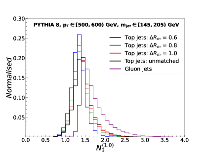
Figure 8: Normalised $N_{3}^{(1.0)}$ distribution of top jets for $\Delta R_{m}$ = 0.6, 0.8, 1.0, unmatched top jets, and gluon jets.

$p_{T}^{J}\in[500,600)$ GeV
Matching radius $\Delta R_{m}$	$m_{jet}$, N-Series: $N_{2}^{(\beta)},~{}N_{3}^{(\beta)}$ ($\beta$ = 1.0, 2.0)
	unpruned		pruned: $z_{cut}=0.1,~{}r_{cut}=0.5$		pruned & unpruned
	Test Accuracy	AUC	Test Accuracy	AUC	Test Accuracy	AUC
0.6	0.916	0.974	0.894	0.961	0.923	0.978
0.8	0.896	0.962	0.875	0.947	0.906	0.968
1.0	0.882	0.952	0.864	0.938	0.892	0.960
unmatched	0.832	0.911	0.819	0.896	0.843	0.921

Table 7: Test accuracy and AUC of XGBOOST trained with $m_{jet}$ and ratios from the N-Series, in the unpruned, pruned, and combined scenario. The rows refer to the different matching criteria for top jets used to train and test the model.

Now to quantify our results better, we introduce the Receiver-Operating-Characteristics (ROC) curves of the six different taggers for pruned and unpruned top jets. The top left panel of Figure 9 shows the ROC curves of the six taggers for unpruned top jets with $\Delta R_{m}$ = 1.0. For moderate top tagging efficiencies, $N$-Subjettiness gives the best performance, followed by U-Series. Table 8 shows the background rejection for a top tagging efficiency of 30$\%$ and 60$\%$. In the top right panel of Figure 9, we see that for all signal efficiencies, the $N$-Subjettiness tagger trained $\Delta R_{m}$ = 0.6 top jets performs the best, while the unmatched top samples cause the worst performance. The two panels in the bottom panel of Figure 9 compare the performance of N-Series and $N$-Subjettiness when using unpruned, pruned, and combined sets of variables. While $N$-Subjettiness has a larger AUC than N-Series overall, the latter shows a more discernible improvement after combining the unpruned with the pruned set.

On testing the $N$-Subjettiness tagger on a dataset containing only unpruned, $\Delta R_{m}$ = 1.0 top jets with $p_{T}\in[500,600)$ GeV, the test accuracy for top jets is 0.858. When tested on unpruned, $\Delta R_{m}$ = 1.0 top jets with $p_{T}\in[500,600)$ GeV that were initially generated with $p_{T,t}$ > 600 GeV, the test accuracy drops by 0.7$\%$ to 0.852. This shows that the set of $N$-Subjettiness variables, when used to train a XGBOOST-based tagger, gives a robust performance even when the top quark had a higher energy initially and the final jet loses energy to fall within the same energy bin.

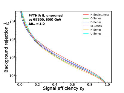
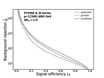
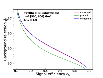
Figure 9: Top left: ROC curves of XGBOOST trained with the six series of variables for unpruned gluon jets and top jets with $\Delta R_{m}$ = 1.0. Top right: ROC curves of XGBOOST trained with the $N$-Subjettiness ratios for unpruned jets with different $\Delta R_{m}$. Bottom left: ROC curves of XGBOOST trained with the N-Series of variables for unpruned, pruned, and combined set of gluon jets and top jets with $\Delta R_{m}$ = 1.0. Bottom right: ROC curves of XGBOOST trained with the $N$-Subjettiness ratios for unpruned, pruned, and combined sets of variables for gluon jets and top jets with $\Delta R_{m}$ = 1.0.

$p_{T}^{J}\in[500,600)$ GeV, $\Delta R_{m}$ = 1.0, unpruned jets
Tagger	$\epsilon_{S}$	1/$\epsilon_{B}$	$\epsilon_{S}$	1/$\epsilon_{B}$
$N$-Subjettiness	0.30	390	0.60	58
C-Series	0.30	281	0.60	39
D-Series	0.30	286	0.60	48
M-Series	0.30	324	0.60	45
N-Series	0.30	246	0.60	34
U-Series	0.30	345	0.60	51

Table 8: Background rejection (1/$\epsilon_{B}$) at 30$\%$ and 60$\%$ signal efficiencies ($\epsilon_{S}$) for six taggers trained with the six series of variables for unpruned top jets and gluon jets with $\Delta R_{m}$ = 1.0 for top jets.

Having constructed the six small sets of taggers with XGBOOST, we try to interpret the results in the next section.

4 SHAP as a method of interpretation

Each feature is a valuable tool that helps the model better identify a jet, but some features play a more critical role than others. Therein lies the usefulness of feature importances. Feature importances can be either global or local. Global feature importance calculates how useful a feature is throughout the entire dataset. Local feature importance is the same for a single prediction (an individual data point or event).

Among various methods used for interpreting a model, we choose to use SHAPDBLP:journals/corr/LundbergL17 . Developed by S. Lundberg and S. Lee, it is a local feature attribution method based on Shapley values Shapley+2016+307+318 . A Shapley value is a quantity designed in the context of game theory to calculate a player’s contribution to a game of $n$ such players. The game has a fixed outcome. This is done by calculating the game’s outcome when one player is removed. The difference between the game’s outcome with and without the player present is a measure of how good that player is. In other words, Shapley values calculate the importance of a feature by determining how good a model is in predicting a particular class when the feature is present versus when it is absent from the list of features. For one feature, it considers not only the feature itself but also the combinations possible among the list of features since there might be correlations among them. The Shapley values are calculated using the following formula DBLP:journals/corr/LundbergL17 ; DBLP:journals/corr/abs-1802-03888 .

$$\phi_{i}=\sum_{S\subseteq N\setminus\{i\}}\frac{|S|!(M-|S|-1)!}{M!}[f_{x}(S\cup\{i\})-f_{x}(S)]$$ (21)

Here, $i$ is the feature for which SHAP value is being calculated, $N$ is the set of all features, $M$ is the total number of features. $S$ is a subset of $N$ that does not include $i$. The function $f_{x}$ is the model prediction. Thus, the algorithm computes a weighted sum of the differences in model prediction outcomes with and without the $i^{th}$ feature for all possible arrangements of the subset $S$.

After the decision trees are trained, we use the package shap to calculate the SHAP values for each feature using the test samples. To compute the SHAP values, shap uses TreeExplainerDBLP:journals/corr/abs-1905-04610 , which is a faster algorithm to estimate SHAP values for tree models. The classification result for each event is equivalent to the total SHAP values of all the features in that specific event. We obtain a mean of the events’ absolute SHAP values by averaging over all of the events. The influence of a variable in categorizing an event as a top or a gluon jet increases with the SHAP value. Figure 10 shows, for every XGBOOST model trained on unpruned, $\Delta R_{m}$ = 1.0 jets with six different sets of variables, the features in decreasing order of importance based on the average of their absolute SHAP values over the entire dataset.

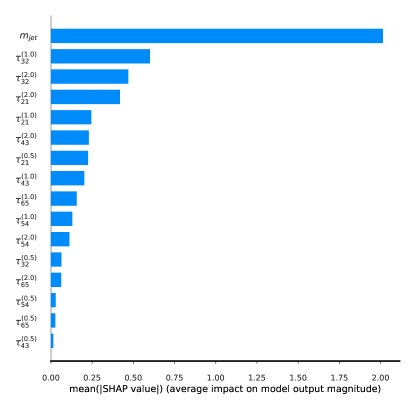
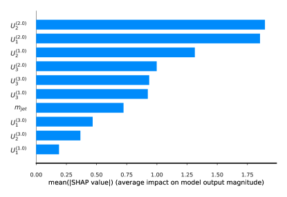
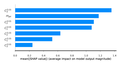
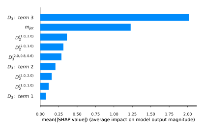
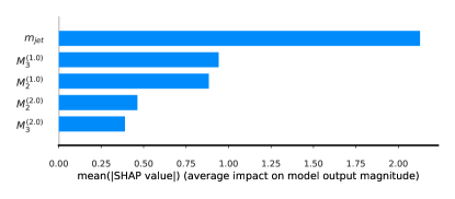
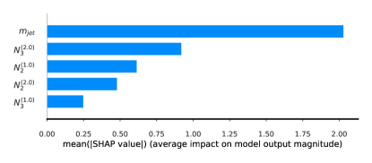
Figure 10: Bar plots depicting the hierarchy of feature importance. Each panel from the top left in the first row to the bottom right in the third row shows the feature importance calculated by SHAP for $N$-Subjettiness, U, C, D, M, and N series consecutively. The dataset contains unpruned top and gluon jets with $\Delta R_{m}$ = 1.0 for top jets.

The model trained with the $N$-Subjettiness series of features has $m_{jet}$ as the most important feature. In other words, $m_{jet}$ contributes the most to the model’s output score, followed by $\tau_{32}^{(1.0)}$, $\tau_{32}^{(2.0)}$, $\tau_{21}^{(2.0)}$, and $\tau_{21}^{(1.0)}$. Higher $N$-Subjettiness ratios are less important in classifying three-pronged jets from QCD. Apart from the U-Series, $m_{jet}$ acquires a high SHAP score in all the models. For the D-Series, the term that has the highest feature importance is $D_{3}:~{}term~{}3$,

$$\frac{e_{4}^{(\gamma)}(e_{2}^{(\alpha)})^{\frac{2\beta}{\gamma}-\frac{\gamma}{\alpha}}}{e_{3}^{(\beta)})^{2}}$$ (22)

This term corresponds to the three-prong phase space where a soft emission has a $p_{T}$ fraction that is parametrically much smaller than the opening angle. In the case of the U-Series, the 2-point correlator has the highest contribution.

4.1 Constructing a hybrid tagger

We first combine the features from all six sets into an extensive set of 49 features and use them for training our decision tree with unpruned jets having $\Delta R_{m}$ = 1.0. When applied to our test dataset, this model gives a test accuracy of 0.904 and an AUC of 0.967. We select the 15 highest-ranked features using SHAP to form a small hybrid set of tagger variables. These 15 features, in order of decreasing importance, are listed in Figure 11.

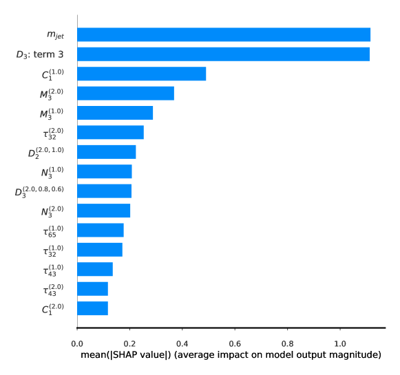
Figure 11: Bar plot depicting the hierarchy of feature importance for the hybrid tagger consisting of the top 15 variables from all six sets combined. The dataset contains unpruned top and gluon jets with $\Delta R_{m}$ = 1.0 for top jets.

The $N$-Subjettiness ratios, when used in combination with the ECFs, have a more minor contribution than the latter, although, in Section 3, we saw that they yielded the best results out of all the sets. With this smaller set, we obtain a test accuracy of 0.902 and an AUC of 0.966, which is only 0.1-0.2$\%$ degradation from earlier. The U-Series of variables, which showed similar performance as $N$-Subjettiness previously, do not make it to the list of the fifteen most important features.

Instead of looking at just the feature importance as an average over all data points, we can also plot the SHAP value of each feature for individual data points. Figure 12 shows a summary plot. Each point on the plot represents an actual data point. The x-axis shows the SHAP value computed for each point and a particular feature on the y-axis. Positive SHAP values give the impact of a feature on classifying the data point as positive or 1 or, in our terms, a "top jet". Similarly, negative SHAP values push the decision towards the negatively labeled, or 0, or "QCD jet" class. The higher the absolute value of SHAP, the more impact that variable has in classification. The colour gradient from blue to red indicates the variation in the feature’s value from low to high. For example, in Figure 12, the most important variable is $m_{jet}$. The high values of $m_{jet}$ push the decision towards "top-like", and the low values of $m_{jet}$ push the decision towards "QCD-like". The dense regions in each line show that most data points have similar SHAP values.

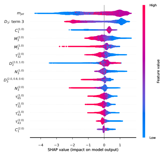
Figure 12: A summary plot showing the variation of SHAP values with the input feature values for the hybrid tagger consisting of the top 15 variables from all six sets combined. The dataset contains unpruned top and gluon jets with $\Delta R_{m}$ = 1.0 for top jets.

To understand how a feature value impacts the model prediction for each data point, we can plot a scatter plot between a feature value and the SHAP value. Figure 13 shows such a dependence plot, that shows the change in a feature’s SHAP value with respect to the feature’s actual value. A dependence plot is a detailed picture of the beeswarm plot in Figure 12. The variation of colour (red and blue) in each dependence plot shows the interaction of the feature with a second feature shown on the right. We can derive the following trends by looking at these plots.

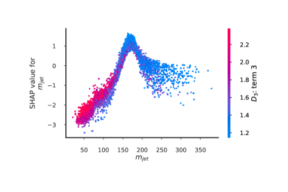
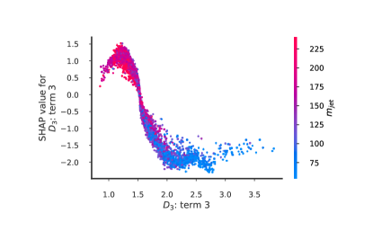
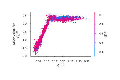
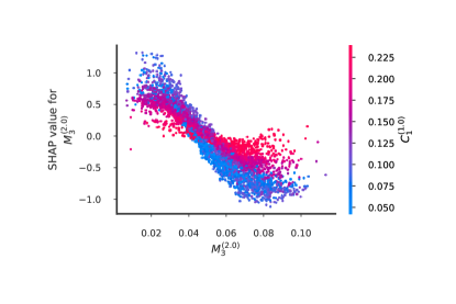
Figure 13: Dependence plots of 5000 test events, of the four most important input features from Figure 11. The x-axis shows a variable’s actual value, while the y-axis shows the SHAP values for each data point. The dataset contains unpruned top and gluon jets with $\Delta R_{m}$ = 1.0 for top jets.

• SHAP value increases with an increase in $m_{jet}$, then reaches the highest $\sim 1$ near the top mass window and decreases for higher values of $m_{jet}$. Low values of $m_{jet}$ are populated by events with high values of $D_{3}$: term 3. At higher values of jet mass, the points are more dispersed, which means there is some other interaction at play.

• When $D_{3}:~{}term~{}3\lesssim 1.5$, the events have a high SHAP value meaning they are more top-like. These events also have moderate to high $m_{jet}$ values.

• SHAP values of $C_{1}^{(1.0)}$ increase from -2.0 to 0.5 with increasing $C_{1}^{(1.0)}$, after which they appear to be constant. $C_{1}^{(1.0)}$ identifies gluon jets very accurately. When $C_{1}^{(1.0)}\gtrsim 0.15$, low values of $\tau_{32}^{(1.0)}$ predict a more top-like nature of the events.

• Low $M_{3}^{(2.0)}$ result in higher SHAP values, especially if $C_{1}^{(1.0)}$ is low too. However, when $M_{3}^{(2.0)}\gtrsim 0.05$, the opposite happens, and low $C_{1}^{(1.0)}$ pushes the prediction to be more QCD-like.

4.2 Interaction effects in SHAP

While computing SHAP values, the algorithm forms coalitions between the features. We can gain more knowledge about the data if we look into the pairwise interactions of features. Given two features $i,j$ out of N input features, SHAP can compute the interaction effect between the two using the Shapley interaction index DBLP:journals/corr/abs-1802-03888 .

$$\Phi_{i,j}=\sum_{S\subseteq N\setminus\{i,j\}}\frac{|S|!(M-|S|-2)!}{2(M-1)!}\delta_{ij}(S),$$ (23)

where $i\neq j$, and

$$\delta_{ij}(S)=[f_{x}(S\cup\{i,j\})-f_{x}(S\cup\{i\})-f_{x}(S\cup\{j\})-f_{x}(S)]$$ (24)

Thus, the interaction effect is calculated by subtracting the contribution of feature $i$ without $j$ present and feature $j$ without $i$ present from the contribution of the pair ${i,j}$ in the coalition. In other words, it can tell us how the effect of $i$ on the prediction might also be affected by $j$. The interaction effect is calculated as $\phi_{ij}=\phi_{ji}$.

The main effect of a feature can be obtained if its interaction with all other features is subtracted from its total contribution (SHAP value).

$$\Phi_{i,i}=\phi_{i}-\sum_{j\neq i}\Phi_{i,j}$$ (25)

SHAP gives the interaction values for each data point in the form of a matrix of N x N features. Figure 14 represents the interaction values between the features.

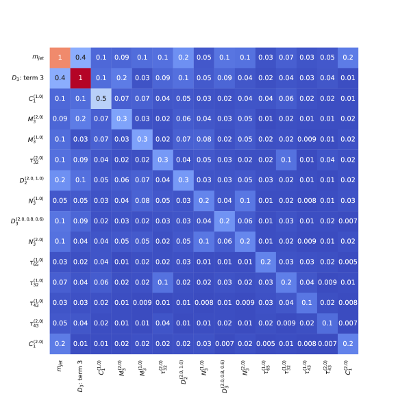
Figure 14: 15 X 15 matrix showing the interaction effects between features of the hybrid tagger. The dataset contains unpruned top and gluon jets with $\Delta R_{m}$ = 1.0 for top jets.

The diagonal of the plot shows the main effects, while the off-diagonal plots show the interaction effects between two features. For example, $m_{jet}^{JH}$ has the most interaction with $D_{3}$: term 3. The total SHAP value of a feature is the sum of the main and interaction effects.

5 Conclusion

In this paper, we study the effects of matching the parton level top and its decay products to the final top jet on the kinematic variables reconstructed to discriminate between top jets and QCD. The parton that carries a significant fraction of the $p_{T}$ of its parent top lies closer to it. Jets matched with a small radius contains final state particles with more $p_{T}$. This effect also percolates to the reconstruction level.

We categorize the top jet samples according to three different matching radii: $\Delta R_{m}$ = 0.6, 0.8, 1.0, and the ones that do not undergo matching are categorized as unmatched. We show that the kinematic distributions of top jets with smaller $\Delta R_{m}$ have lesser overlap with the background. We construct standard top tagging variables with $N$-Subjettiness ratios and Energy Correlation Functions. For top tagging purposes, we use a decision tree algorithm, XGBOOST, and feed six different series of variables: $N$-Subjettiness, C-Series, D-Series, M-Series, N-Series, and U-Series, as the input features to our binary classifier. $N$-Subjettiness gives the best test accuracy and AUC among the six series. We see that the XGBOOST model performs the best top-QCD classification with $\Delta R_{m}$ = 0.6 top jets, and the performance degrades with an increase in $\Delta R_{m}$, becoming the worst with unmatched top jets.

With pruned jets, series with ECF observables give better results than $N$-Subjettiness. However, pruning causes taggers to classify top and gluon jets less accurately. Throughout the analysis, we select jets with $p_{T}\in[500,600)$ GeV. Events generated with high $p_{T}$ of 600 GeV lose energy and pass the specified $p_{T}$ selection criteria. Such top jets, when used to test the $N$-Subjettiness tagger, cause the tagger’s performance on top jets to degrade by only 0.7$\%$, which implies its robustness irrespective of the initial top quark energy, given the final jet falls within the same energy bin.

Having constructed the taggers using XGBOOST, we use SHAP to interpret the results. SHAP assigns a score to all the features according to their contribution to the model’s classification output. In all the taggers except for the one with the U-Series of variables, $m_{jet}$ attains high importance. In the D-Series tagger, the third term of the generalized $D_{3}$ variable is the most important feature. This term appears again at a high rank when we combine all the variables into one single top tagger. From the dependence plots, we see which regions of the feature space are selected by the XGBOOST model to classify an event as a top jet or a gluon jet. The final probability score for an event can be understood in terms of the SHAP values themselves, which are calculated according to the value that the features assume.

References

- (1) G. ’t Hooft, Naturalness, chiral symmetry, and spontaneous chiral symmetry breaking, NATO Sci. Ser. B 59 (1980) 135–157.
- (2) E. Gildener and S. Weinberg, Symmetry Breaking and Scalar Bosons, Phys. Rev. D 13 (1976) 3333.
- (3) L. Susskind, Dynamics of Spontaneous Symmetry Breaking in the Weinberg-Salam Theory, Phys. Rev. D 20 (1979) 2619–2625.
- (4) N. Arkani-Hamed, A. G. Cohen, and H. Georgi, Electroweak symmetry breaking from dimensional deconstruction, Phys. Lett. B 513 (2001) 232–240, [hep-ph/0105239].
- (5) N. Arkani-Hamed, A. G. Cohen, E. Katz, and A. E. Nelson, The Littlest Higgs, JHEP 07 (2002) 034, [hep-ph/0206021].
- (6) D. E. Kaplan, K. Rehermann, M. D. Schwartz, and B. Tweedie, Top Tagging: A Method for Identifying Boosted Hadronically Decaying Top Quarks, Phys. Rev. Lett. 101 (2008) 142001, [arXiv:0806.0848].
- (7) T. Plehn, G. P. Salam, and M. Spannowsky, Fat Jets for a Light Higgs, Phys. Rev. Lett. 104 (2010) 111801, [arXiv:0910.5472].
- (8) T. Plehn, M. Spannowsky, M. Takeuchi, and D. Zerwas, Stop Reconstruction with Tagged Tops, JHEP 10 (2010) 078, [arXiv:1006.2833].
- (9) T. Plehn, M. Spannowsky, and M. Takeuchi, How to Improve Top Tagging, Phys. Rev. D 85 (2012) 034029, [arXiv:1111.5034].
- (10) J. Thaler and K. Van Tilburg, Identifying Boosted Objects with N-subjettiness, JHEP 03 (2011) 015, [arXiv:1011.2268].
- (11) A. J. Larkoski, G. P. Salam, and J. Thaler, Energy Correlation Functions for Jet Substructure, JHEP 06 (2013) 108, [arXiv:1305.0007].
- (12) I. Moult, L. Necib, and J. Thaler, New Angles on Energy Correlation Functions, JHEP 12 (2016) 153, [arXiv:1609.07483].
- (13) L. G. Almeida, M. Backović, M. Cliche, S. J. Lee, and M. Perelstein, Playing Tag with ANN: Boosted Top Identification with Pattern Recognition, JHEP 07 (2015) 086, [arXiv:1501.05968].
- (14) G. Kasieczka, T. Plehn, M. Russell, and T. Schell, Deep-learning Top Taggers or The End of QCD?, JHEP 05 (2017) 006, [arXiv:1701.08784].
- (15) A. Butter, G. Kasieczka, T. Plehn, and M. Russell, Deep-learned Top Tagging with a Lorentz Layer, SciPost Phys. 5 (2018), no. 3 028, [arXiv:1707.08966].
- (16) S. Macaluso and D. Shih, Pulling Out All the Tops with Computer Vision and Deep Learning, JHEP 10 (2018) 121, [arXiv:1803.00107].
- (17) L. Moore, K. Nordström, S. Varma, and M. Fairbairn, Reports of My Demise Are Greatly Exaggerated: -subjettiness Taggers Take On Jet Images, SciPost Phys. 7 (2019), no. 3 036, [arXiv:1807.04769].
- (18) A. Butter et al., The Machine Learning landscape of top taggers, SciPost Phys. 7 (2019) 014, [arXiv:1902.09914].
- (19) T. S. Roy and A. H. Vijay, A robust anomaly finder based on autoencoders, arXiv:1903.02032.
- (20) S. Diefenbacher, H. Frost, G. Kasieczka, T. Plehn, and J. M. Thompson, CapsNets Continuing the Convolutional Quest, SciPost Phys. 8 (2020) 023, [arXiv:1906.11265].
- (21) A. Chakraborty, S. H. Lim, M. M. Nojiri, and M. Takeuchi, Neural Network-based Top Tagger with Two-Point Energy Correlations and Geometry of Soft Emissions, JHEP 07 (2020) 111, [arXiv:2003.11787].
- (22) S. Bhattacharya, M. Guchait, and A. H. Vijay, Boosted top quark tagging and polarization measurement using machine learning, Phys. Rev. D 105 (2022), no. 4 042005, [arXiv:2010.11778].
- (23) S. H. Lim and M. M. Nojiri, Morphology for jet classification, Phys. Rev. D 105 (2022), no. 1 014004, [arXiv:2010.13469].
- (24) F. A. Dreyer and H. Qu, Jet tagging in the Lund plane with graph networks, JHEP 03 (2021) 052, [arXiv:2012.08526].
- (25) J. A. Aguilar-Saavedra, Pulling the Higgs and top needles from the jet stack with feature extended supervised tagging, Eur. Phys. J. C 81 (2021), no. 8 734, [arXiv:2102.01667].
- (26) M. Andrews et al., End-to-end jet classification of boosted top quarks with the CMS open data, EPJ Web Conf. 251 (2021) 04030, [arXiv:2104.14659].
- (27) F. A. Dreyer, R. Grabarczyk, and P. F. Monni, Leveraging universality of jet taggers through transfer learning, Eur. Phys. J. C 82 (2022), no. 6 564, [arXiv:2203.06210].
- (28) I. Ahmed, A. Zada, M. Waqas, and M. U. Ashraf, Application of deep learning in top pair and single top quark production at the LHC, arXiv:2203.12871.
- (29) J. M. Munoz, I. Batatia, and C. Ortner, BIP: Boost Invariant Polynomials for Efficient Jet Tagging, arXiv:2207.08272.
- (30) ATLAS Collaboration, G. Aad et al., Search for resonances in fully hadronic final states in collisions at = 13 TeV with the ATLAS detector, JHEP 10 (2020) 061, [arXiv:2005.05138].
- (31) ATLAS Collaboration, Boosted hadronic vector boson and top quark tagging with ATLAS using Run 2 data, tech. rep., CERN, Geneva, 2020.
- (32) ATLAS Collaboration, Constituent-Based Top-Quark Tagging with the ATLAS Detector, tech. rep., CERN, Geneva, 2022.
- (33) CMS Collaboration, S. Chatrchyan et al., Search for Anomalous Production in the Highly-Boosted All-Hadronic Final State, JHEP 09 (2012) 029, [arXiv:1204.2488]. [Erratum: JHEP 03, 132 (2014)].
- (34) CMS Collaboration, A. M. Sirunyan et al., Search for resonances in highly boosted lepton+jets and fully hadronic final states in proton-proton collisions at TeV, JHEP 07 (2017) 001, [arXiv:1704.03366].
- (35) CMS Collaboration, A. M. Sirunyan et al., Search for top squark production in fully-hadronic final states in proton-proton collisions at 13 TeV, Phys. Rev. D 104 (2021), no. 5 052001, [arXiv:2103.01290].
- (36) C. Grojean, A. Paul, and Z. Qian, Resurrecting with kinematic shapes, JHEP 04 (2021) 139, [arXiv:2011.13945].
- (37) L. Bradshaw, S. Chang, and B. Ostdiek, Creating simple, interpretable anomaly detectors for new physics in jet substructure, Phys. Rev. D 106 (2022), no. 3 035014, [arXiv:2203.01343].
- (38) A. Khot, M. S. Neubauer, and A. Roy, A Detailed Study of Interpretability of Deep Neural Network based Top Taggers, arXiv:2210.04371.
- (39) R. Das, G. Kasieczka, and D. Shih, Feature Selection with Distance Correlation, arXiv:2212.00046.
- (40) T. Chen and C. Guestrin, Xgboost: A scalable tree boosting system, CoRR abs/1603.02754 (2016) [arXiv:1603.02754].
- (41) S. M. Lundberg and S. Lee, A unified approach to interpreting model predictions, CoRR abs/1705.07874 (2017) [arXiv:1705.07874].
- (42) S. M. Lundberg, G. G. Erion, and S. Lee, Consistent individualized feature attribution for tree ensembles, CoRR abs/1802.03888 (2018) [arXiv:1802.03888].
- (43) S. M. Lundberg, G. G. Erion, H. Chen, A. J. DeGrave, J. M. Prutkin, B. Nair, R. Katz, J. Himmelfarb, N. Bansal, and S. Lee, Explainable AI for trees: From local explanations to global understanding, CoRR abs/1905.04610 (2019) [arXiv:1905.04610].
- (44) L. S. Shapley, 17. A Value for n-Person Games, pp. 307–318. Princeton University Press, 2016.
- (45) A. S. Cornell, W. Doorsamy, B. Fuks, G. Harmsen, and L. Mason, Boosted decision trees in the era of new physics: a smuon analysis case study, JHEP 04 (2022) 015, [arXiv:2109.11815].
- (46) D. Alvestad, N. Fomin, J. Kersten, S. Maeland, and I. Strümke, Beyond Cuts in Small Signal Scenarios – Enhanced Sneutrino Detectability Using Machine Learning, arXiv:2108.03125.
- (47) CMS Collaboration, A. Tumasyan et al., Evidence for WW/WZ vector boson scattering in the decay channel qq produced in association with two jets in proton-proton collisions at s=13 TeV, Phys. Lett. B 834 (2022) 137438, [arXiv:2112.05259].
- (48) C. Grojean, A. Paul, Z. Qian, and I. Strümke, Lessons on interpretable machine learning from particle physics, Nature Rev. Phys. 4 (2022), no. 5 284–286, [arXiv:2203.08021].
- (49) A. Adhikary, S. Banerjee, R. K. Barman, B. Batell, B. Bhattacherjee, C. Bose, Z. Qian, and M. Spannowsky, Prospects for Exotic Decays in Single and Di-Higgs Production at the LHC and Future Hadron Colliders, arXiv:2211.07674.
- (50) J. Alwall, M. Herquet, F. Maltoni, O. Mattelaer, and T. Stelzer, MadGraph 5 : Going Beyond, JHEP 06 (2011) 128, [arXiv:1106.0522].
- (51) J. Alwall, R. Frederix, S. Frixione, V. Hirschi, F. Maltoni, O. Mattelaer, H. S. Shao, T. Stelzer, P. Torrielli, and M. Zaro, The automated computation of tree-level and next-to-leading order differential cross sections, and their matching to parton shower simulations, JHEP 07 (2014) 079, [arXiv:1405.0301].
- (52) T. Sjostrand, S. Mrenna, and P. Z. Skands, A Brief Introduction to PYTHIA 8.1, Comput. Phys. Commun. 178 (2008) 852–867, [arXiv:0710.3820].
- (53) DELPHES 3 Collaboration, J. de Favereau, C. Delaere, P. Demin, A. Giammanco, V. Lemaître, A. Mertens, and M. Selvaggi, DELPHES 3, A modular framework for fast simulation of a generic collider experiment, JHEP 02 (2014) 057, [arXiv:1307.6346].
- (54) A. Buckley, J. Ferrando, S. Lloyd, K. Nordström, B. Page, M. Rüfenacht, M. Schönherr, and G. Watt, LHAPDF6: parton density access in the LHC precision era, Eur. Phys. J. C 75 (2015) 132, [arXiv:1412.7420].
- (55) Y. L. Dokshitzer, G. D. Leder, S. Moretti, and B. R. Webber, Better jet clustering algorithms, JHEP 08 (1997) 001, [hep-ph/9707323].
- (56) M. Cacciari and G. P. Salam, Dispelling the myth for the jet-finder, Phys. Lett. B 641 (2006) 57–61, [hep-ph/0512210].
- (57) M. Cacciari, G. P. Salam, and G. Soyez, FastJet User Manual, Eur. Phys. J. C 72 (2012) 1896, [arXiv:1111.6097].
- (58) S. D. Ellis, C. K. Vermilion, and J. R. Walsh, Recombination Algorithms and Jet Substructure: Pruning as a Tool for Heavy Particle Searches, Phys. Rev. D 81 (2010) 094023, [arXiv:0912.0033].
- (59) A. J. Larkoski, I. Moult, and D. Neill, Power Counting to Better Jet Observables, JHEP 12 (2014) 009, [arXiv:1409.6298].
- (60) A. J. Larkoski, I. Moult, and D. Neill, Building a Better Boosted Top Tagger, Phys. Rev. D 91 (2015), no. 3 034035, [arXiv:1411.0665].
- (61) A. J. Larkoski, I. Moult, and D. Neill, Analytic Boosted Boson Discrimination, JHEP 05 (2016) 117, [arXiv:1507.03018].