The Belle Collaboration

 
Search for a heavy neutrino in $\tau$ decays at Belle

Abstract

We report on a search for a heavy Majorana neutrino in the decays $\tau^{-}\to\pi^{-}\nu_{h}$, $\nu_{h}\to\pi^{\pm}\ell^{\mp}$, $\ell=e,\mu$. The results are obtained using the full data sample of $988\,\mathrm{fb}^{-1}$ collected with the Belle detector at the KEKB asymmetric energy $e^{+}e^{-}$ collider, which contains $912\times 10^{6}$ $\tau\tau$ pairs. We observe no significant signal and set 95% CL upper limits on the couplings of the heavy right-handed neutrinos to the conventional SM left-handed neutrinos in the mass range $0.2-1.6\,\textrm{GeV}/c^{2}$. This is the first study of a mixed couplings of heavy neutrinos to $\tau$ leptons and light-flavor leptons.

In the Standard model (SM), neutrinos are strictly massless since there are no right-handed neutrino components. However, experimental data on neutrino oscillations conclusively show that neutrinos are massive [1], though neutrino mass measurements show that their masses are very small [2]. One approach to resolve this disagreement is to include right-handed neutrinos, also known as sterile neutrinos, heavy neutrinos, or heavy neutral leptons (HNL), into the model. Such particles do not participate in any of the weak, strong, and electromagnetic interactions; if we exclude gravitation, the only way they interact with matter is via mixing with left-handed neutrinos. Singlet right-handed neutrinos may also have Majorana mass, naturally explaining the smallness of the observed neutrino masses via the so-called “see-saw” mechanism [3]. One example of the models realizing such a mechanism is $\nu$MSM [4]. It introduces three right-handed singlet HNLs, so that every left-handed particle gets its right-handed counterpart, and manages to explain neutrino oscillations, dark matter existence, and baryogenesis with the same set of parameters. HNLs also appear in other extensions of the SM; see a review in Ref. [5].

In general, neutrino flavor eigenstates need not to coincide with the mass eigenstates but may be related through a unitary transformation, similar to that in the quark sector:

$$\nu_{\alpha}=\sum_{i}{U_{\alpha i}\nu_{i}},\quad\alpha=e,\mu,\tau,...,\,i=1,2,3,4,...$$ (1)

where Greek (Latin) indexes denote flavor (mass) eigenstates. The coupling of the HNLs to charged or neutral currents of flavor $\alpha$ is characterized by the quantities $U_{\alpha 4}$, $U_{\alpha 5}$ etc, which we denote for convenience as $U_{\alpha}$. A generic HNL is denoted by $\nu_{h}$. Its production and decay diagrams are shown in Fig. 1. Existing experimental results are reviewed and discussed in Ref. [5].

In our previous analysis [6] we searched for the decays of HNLs produced in $B$ decays. No signal was found and upper limits on $|U_{e}|^{2}$, $|U_{\mu}|^{2}$ and $|U_{e}||U_{\mu}|$ as functions of the mass of the HNL were set.

In this analysis, we reconstruct $\tau^{-}\to\pi^{-}_{p}\nu_{h}$ decays, where $\pi_{p}$ refers to the “prompt pion” and the HNL decays into a pion-lepton pair in the detector volume: $\nu_{h}\to\pi^{\pm}\ell^{\mp}$, $\ell=e,\mu$ (the charge-conjugate decay mode being included throughout this Letter). Both combinations of $\tau$ and $\ell$ charges are retained for further analysis. In the final state, we have two pions and a lepton: $\pi^{-}_{p}\pi^{\pm}\ell^{\mp}$.

Following [7, 8], we interpret the result in terms of the minimal realistic model with two quasi-degenerate HNLs with close masses and couplings and not trivial $U_{\alpha}$. When two HNL masses are not exactly the same, HNL oscillations occur and we consider two extreme cases: the “Dirac-like limit”, where only lepton-number conserving final states are allowed, and the “Majorana-like limit”, where lepton-number violating final states are also allowed with the same branching fractions. The ratio of different $U_{\alpha}$ is determined from the neutrino oscillation data. In the normal hierarchy case (NH), the relative mixing coefficients $x_{\alpha}\equiv|U_{\alpha}|^{2}/|U|^{2}$, $|U|^{2}=\sum_{\alpha}|U_{\alpha}|^{2}$ $(\alpha=e,\mu,\tau)$ are taken to be $x_{e}=0.06$, $x_{\mu}=0.48$ and $x_{\tau}=0.46$; for the inverted hierarchy case (IH), we use the values $x_{\alpha}=1/3$ $(\alpha=e,\mu,\tau)$ [7].

A distinctive feature of the HNL is its long lifetime. We can estimate it as $c\tau\sim|U|^{-2}M(\nu_{h})^{-5}$ [9]: for $M(\nu_{h})=1\,\textrm{GeV}/c^{2}$ and $|U|^{2}=10^{-4}$, the lifetime is $c\tau\sim 20\,\textrm{m}$; thus, a $\pi\ell$ pair forms a vertex displaced from the interaction point (IP). BaBar [10] and Belle [11] previously searched for $\tau\to\ell hh^{\prime}$ decays; however, both analyses required all tracks to originate in the vicinity of the IP. For the long-lived HNL, this greatly reduces the reconstruction efficiency. In contrast, we do not impose such a requirement on the HNL daughters.

Results presented here are based on all available Belle data, including on-resonance, off-resonance and energy scans. The collision energy is around 10.58 GeV. The total integrated luminosity is $988\,\mathrm{fb}^{-1}$ [12] and the total number of $\tau^{+}\tau^{-}$ pairs is calculated using direct production cross sections [13] and $\Upsilon(NS)$ branching fractions to be $N_{\tau\tau}=(912\pm 13)\times 10^{6}$, where the error arises from the luminosity measurement.

The Belle detector is a large-solid-angle magnetic spectrometer that consists of a silicon vertex detector (SVD), a 50-layer central drift chamber (CDC), an array of aerogel threshold Cherenkov counters (ACC), a barrel-like arrangement of time-of-flight scintillation counters (TOF), and an electromagnetic calorimeter comprised of CsI(Tl) crystals (ECL) located inside a super-conducting solenoid coil that provides a 1.5 T magnetic field. An iron flux-return located outside of the coil is instrumented to detect $K_{L}^{0}$ mesons and to identify muons (KLM). The detector is described in detail elsewhere [14].

To study backgrounds, we use the following Monte Carlo (MC) simulated samples: $e^{+}e^{-}\to q\bar{q}$ $(q=u,d,s,c,b)$, $e^{+}e^{-}$, $\mu^{+}\mu^{-}$, $\tau^{+}\tau^{-}$ and two-photon processes ($e^{+}e^{-}\to e^{+}e^{-}\ell^{+}\ell^{-}$, $e^{+}e^{-}q\bar{q}$). Background processes are generated by EvtGen [15], BHLUMI [18], KKMC [16], KKMC ($\tau\tau$ production) and TAUOLA ($\tau$ decay) [17], and AAFH [19], respectively. We use signal MC samples generated with different HNL masses of $M(\nu_{h})=0.2\,\textrm{GeV}/c^{2}$ to $1.6\,\textrm{GeV}/c^{2}$ (with $0.1\,\textrm{GeV}/c^{2}$ step) and life times of $c\tau=0.2,0.5,$ and $1.0\,\textrm{m}$ to study the response of the detector and to determine its acceptance and signal efficiency dependence on the neutrino mass and the distance of the decay point from the IP. This efficiency does not depend on $c\tau$ ($|U|^{2}$). Signal MC samples are $\tau^{+}\tau^{-}$ pairs where one of the $\tau$ leptons decays according to the modes under study and the other decays generically. Signal events are generated using EvtGen; radiative corrections are included using PHOTOS [20]. HNLs are produced and decayed uniformly in phase space. GEANT3 [21] is used to model the detector response.

Electrons are identified using the energy and shower profile in the ECL, the light yield in the ACC and the specific ionization energy loss in the CDC ($dE/dx$). This information is used to form an electron ($\mathcal{L}_{e}$) and non-electron ($\mathcal{L}_{\bar{e}}$) likelihood; these are combined into a likelihood ratio $\mathcal{P}_{e}=\mathcal{L}_{e}/(\mathcal{L}_{e}+\mathcal{L}_{\bar{e}})$ [22]. Muons are distinguished from other charged tracks by their range and hit profiles in the KLM. This information is utilized in a likelihood ratio approach [23] similar to the one used for the electron identification.

Charged tracks with laboratory momentum greater than $0.5\,\textrm{GeV}/c$ and electron likelihood ratio $\mathcal{P}_{e}>0.9$ or muon ratio $\mathcal{P}_{\mu}>0.9$ are treated as leptons. These requirements correctly identify leptons with an efficiency of approximately 95% and a misidentification rate of less than 2%. All charged tracks not identified as leptons and satisfying the electron veto ${\cal P}_{e}<0.5$ are treated as pions.

HNL candidates are formed from a pion $\pi$ and a lepton $\ell$ of the opposite sign. The pion and lepton are then fitted to a common vertex. HNL candidates are combined with a prompt pion $\pi_{p}$. The second vertex fit of the HNL candidate and the prompt pion is performed with a vertex constraint to the IP, which is determined run-by-run using charged tracks. The $\chi^{2}$ of both vertex fits is required to be $\chi^{2}/ndf<25$, where $ndf$ is the number of degrees of freedom. Kinematics of the particles are updated after the fits are performed. For the prompt pion, we require the closest distance to IP along the detector symmetry axis ($dz$) to be $|dz|<5\,\textrm{cm}$ and in the transverse plane to be $dr<1\,\textrm{cm}$.

Since the signal $\tau$ lepton is fully reconstructed, we can utilize the kinematic constraint of the known initial four-momentum of the colliding $e^{+}e^{-}$ pair to define $\Delta E\equiv E(\pi_{p}\pi\ell)-E_{\textrm{cm}}$ in the center-of-mass (c.m.) frame of a $\tau$ candidate relative to the beam energy $E_{\textrm{cm}}$. In $\tau$ decays, $\Delta E$ and $M(\pi_{p}\pi\ell)$ are highly correlated; therefore, we use an elliptically shaped requirement, that encompasses $\sim$ 95% efficiency as computed from the signal simulation.

In the rest of the event, we select tracks with $dr<1\,\textrm{cm}$, $|dz|<5\,\textrm{cm}$ and a transverse momentum $p_{t}>0.1\,\textrm{GeV}/c$. We classify clusters in the ECL not associated with charged tracks as photons and require $E(\gamma)>0.05\,\textrm{GeV}$ in the barrel ($32.2^{\circ}<\theta<128.7^{\circ}$), $E(\gamma)>0.1\,\textrm{GeV}$ in the forward endcap ($12.4^{\circ}<\theta<31.4^{\circ}$) and $E(\gamma)>0.15\,\textrm{GeV}$ in the backward endcap ($130.7^{\circ}<\theta<155.1^{\circ}$). Events are separated into two hemispheres by the plane perpendicular to the thrust axis $\vec{n}_{T}$ [24], defined to maximize the thrust magnitude value

$$V_{T}=\frac{\sum|\vec{p}_{i}^{*}\cdot\vec{n}_{T}|}{\sum|\vec{p}_{i}^{*}|},$$ (2)

where $\vec{p}_{i}^{*}$ are momenta of the selected tracks, photons and $\tau$ daughters in the c.m. frame. We require the signal hemisphere to contain no additional tracks besides $\tau$ daughters, and the opposite side to contain one or three tracks with a total charge opposite that of the prompt pion.

We select well-vertexed HNL candidates using $d\phi$, the angle between the momentum vector and decay-vertex vector of the HNL candidate; $dz_{\textrm{vtx}}$, the distance between the daughter tracks at their closest approach in the direction parallel to the beam; and $dr$ for each track. Requirements vary depending on the presence of SVD hits on the tracks and on the HNL candidate flight length. These are summarized in Table 1. The four event types in the Table are I: both neutrino daughter tracks have recorded hits in SVD, II: one of the neutrino daughter tracks has recorded hits in SVD, III: none of the neutrino daughter tracks have recorded hits in SVD, with $M(\nu_{h})\geq 0.8\,\textrm{GeV}/c^{2}$, and IV: no SVD hits and $M(\nu_{h})<0.8\,\textrm{GeV}/c^{2}$. There is a large contamination from the conversion photons $\gamma\to ee$ in the last category.

Table 1: Summary of the vertex requirements.

Type	$d\phi$, rad	$z_{\mathrm{vtx}}$, cm	$dr$, cm
I	$<0.02$	$<0.06$	$>0.07$
II	$<0.024$	$<1.5$	$>0.08$
III	$<0.16$	$<3.0$	$>0.1$
IV	$<0.16$	$<3.0$	$>1.0$

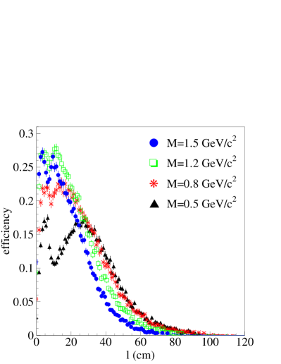
Figure 2: Dependence of the HNL reconstruction efficiency on the neutrino travel distance $l$ for different neutrino masses $M(\nu_{h})$. Efficiency is almost identical for $e$ and $\mu$.

Figure 2 shows the efficiency of HNL reconstruction with all requirements applied as a function of the reconstructed travel distance $l$ for several mass hypotheses.

The number of neutrinos detected by this method is (in units where $\hbar=c=1$) [25]

$$n(\nu_{h}) =2N_{\tau\tau}\ \mathcal{B}(\tau\to\pi\nu_{h})\ \mathcal{B}(\nu_{h}\to\pi\ell)\ \frac{m\Gamma}{p}\int\exp\Big{(}-\frac{m\Gamma l}{p}\Big{)}\varepsilon(m,l)dl$$

$$=|U_{\tau}|^{2}|U_{\ell}|^{2}\ 2N_{\tau\tau}\ f_{1}(m)\ f_{2}(m)\ \frac{m}{p}\int\exp\Big{(}-\frac{m\Gamma l}{p}\Big{)}\varepsilon(m,l)dl,$$ (3)

where $N_{\tau\tau}$ is the number of $\tau\tau$ pairs, $\mathcal{B}(\tau\to\pi\nu_{h})$ is the branching fraction for $\nu_{h}$ production, $\mathcal{B}(\nu_{h}\to\pi\ell)$ is the branching fraction of the reconstructed decay, $m$, $p$ and $\Gamma=\Gamma(m,U)$ are the mass, momentum and full width of the HNL, respectively, and $\varepsilon(m,l)$ is the reconstruction efficiency of the HNL of mass $m$ decaying at a distance $l$ from the IP. The momentum $p$ is approximated by the mean value for a given mass, determined from the signal MC simulation. To factor out the $|U_{\ell}|^{2}$ dependence, we define functions $f_{1,2}(m)$ as $|U_{\tau}|^{2}f_{1}(m)\equiv\mathcal{B}(\tau\to\pi\nu_{h})$ and $|U_{\ell}|^{2}f_{2}(m)\equiv\Gamma(\nu_{h}\to\pi\ell)=\mathcal{B}(\nu_{h}\to\pi\ell)\Gamma$, where $\ell$ denotes the flavor ($e,\ \mu$) of the charged lepton produced in the $\nu_{h}$ decay. Integration is performed over the full volume used to reconstruct the HNL vertex. The expressions for $\mathcal{B}(\tau\to\pi\nu_{h})$, $\Gamma(\nu_{h}\to\pi\ell)$ and the full neutrino width $\Gamma$ are taken from Ref. [26] and require only general assumptions (i.e., they are not specific to the $\nu$MSM model). In the Majorana case $\Gamma(\nu_{h}\to\pi\ell)$ is twice that in the Dirac case. Given number of observed events, we solve Eq.  Search for a heavy neutrino in $\tau$ decays at Belle for the variable $|U|^{2}$ using the relative mixing coefficients $x_{\alpha}$ defined above.

The systematic uncertainties in number of events calculated according to Eq.  Search for a heavy neutrino in $\tau$ decays at Belle are enumerated in Table 2. We estimate the systematic uncertainties of event selection criteria from the differences in their efficiencies obtained in data and MC simulation. Since all particles used in the systematic uncertainty study decay relatively close to the IP compared to the expectation for an HNL, we require where possible that the decay vertices be farther than 4 cm from the IP in the transverse plane to put more weight on large decay lengths. To estimate the systematic uncertainty due to tracking, we compare the number of fully and partially reconstructed $D^{*+}$ decays in the decay chain $D^{*+}\to D^{0}\pi^{+}$, $D^{0}\to K_{S}^{0}\pi^{+}\pi^{-}$, $K_{S}^{0}\to\pi^{+}\pi^{-}$, where in the latter case one of the pions from the $K_{S}^{0}$ is explicitly left unreconstructed. To estimate the systematic uncertainty of the lepton identification, we reconstruct $J/\psi\to\ell^{+}\ell^{-}$, $\ell=e,\mu$ events, where one of the daughter particles is identified as an electron or muon. The difference of the identification efficiency of the other daughter between data and MC simulation is treated as a systematic uncertainty. To estimate the systematic uncertainty of the vertex quality requirements we apply them to $K^{0}_{S}$ decays, which have a topology similar to HNL decays. Signal events were generated using EvtGen, which is not optimized for $\tau$ decays. To estimate the effect of this we prepared two samples of $\tau\tau$ events — one generated with EvtGen and the other with KKMC and TAUOLA — then reconstructed $\tau\to\ell\nu\nu$ decays, where $\ell=e,\mu$, using the same tagging as for the signal events and compared reconstruction efficiency in both cases. The phase space model may not give the correct angle distribution of the HNL. We vary it by reweighting generated events and treat the change as a systematic uncertainty. The calculation uncertainty comes from the efficiency and momentum approximations in Eq.  Search for a heavy neutrino in $\tau$ decays at Belle and was estimated by comparing predicted and observed number of events in different subsets of the signal MC simulation. Systematic uncertainties induced by the fitting procedure were found by varying the signal resolution and background shape within their errors. The theoretical uncertainty arises from uncertainties in the constants used in Eq.  Search for a heavy neutrino in $\tau$ decays at Belle. Correlations between different systematic uncertainties are found to be small and are ignored. All systematic uncertainties are summed in quadrature, leading to total systematic uncertainties of 16% and 12% for the $\pi\pi e$ and $\pi\pi\mu$ modes, respectively. The largest contributions are lepton identification (12% and 6% for the electron and muon identification, respectively) and vertex quality requirements (5.3%).

Table 2: Summary of systematic uncertainties in number of events calculated according to Eq.  Search for a heavy neutrino in $\tau$ decays at Belle.

Requirement	Systematic uncertainty, %
Tracking	1.2
${\cal P}_{e}(\ell)$	12
${\cal P}_{\mu}(\ell)$	6
Vertex quality	5.3
$N_{\tau\tau}$	1.4
Generator	2
Angle distribution	5
Calculation	4
Signal resolution	2.5
Background shape	4
Theoretical	0.35
Total, $e/\mu$	16/12

We study the dependence of the coupling constant $|U|^{2}$ on the HNL mass using simultaneous fit to $\pi\pi e$ and $\pi\pi\mu$ modes taking into account the relative mixing coefficients $x_{\alpha}$ defined above.

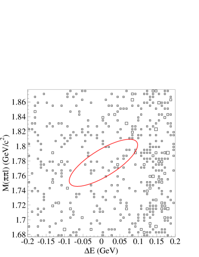
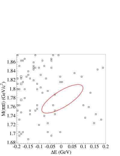
a)	b)

Figure 3: $\Delta E$ vs $M(\pi\pi\ell)$ distributions with all requirements but $\Delta E$ and $M(\pi\pi\ell)$ imposed for $\pi\pi e$ (a) and $\pi\pi\mu$ (b) in data. The signal region is shown as a red ellipse.

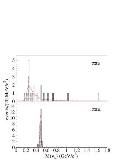
Figure 4: Final distributions of $M(\nu_{h})$ for $\pi\pi e$ and $\pi\pi\mu$ reconstruction modes in data. The filled histograms are for candidates with opposite-charge $\tau$ and $\ell$, while the open histograms are for candidates with same-charge combinations. The curves are the fits with the signal yield fixed at zero.

The $\Delta E$ vs $M(\pi\pi\ell)$ distributions with all requirements but $\Delta E$ and $M(\pi\pi\ell)$ imposed are shown in Fig. 3. The mass distributions after application of all reconstruction requirements are shown in Fig. 4 for the same-charge $\tau$ and $\ell$ (“Dirac-like limit”) and both same- and opposite-charge combinations (“Majorana-like limit”). From the background MC simulation study, we expect to see a wide peak around $\sim 0.2\,\textrm{GeV}/c^{2}$ from the conversion process $\gamma\to e^{+}e^{-}$ in the $\pi\pi e$ mode and a narrow peak from the $K_{S}^{0}\to\pi^{+}\pi^{-}$ process at $\sim 0.48\,\textrm{GeV}/c^{2}$ in the $\pi\pi\mu$ mode. Since the conversion peak is wide, we can distinguish a narrow signal peak from the HNL decay under it, but since the $K_{S}^{0}$ peak is narrow, we exclude the $K_{S}^{0}$ region at $0.464-0.494\,\textrm{GeV}/c^{2}$ from consideration, which corresponds to $\pm 2\sigma$ of the peak width.

The HNL mass is unknown and we search for it in the kinematically accessible region for the mass; for the decays under study, this lies between $M_{\pi}+M_{\ell}$ and $M_{\tau}-M_{\pi}$. We perform a series of binned likelihood fits to the mass distributions using the sum of a Gaussian signal function and background (described below) varying the mass hypothesis in each fit. The neutrino mass is set to the center of a histogram bin which has a width of $2\,\textrm{MeV}/c^{2}$. The signal-shape parameters used in the fits to data are fixed to those obtained by fitting simulated events. The width evolves linearly from $\sim 3\,\textrm{MeV}/c^{2}$ for $M(\nu_{h})=0.2\,\textrm{GeV}/c^{2}$ to $\sim 10\,\textrm{MeV}/c^{2}$ for $M(\nu_{h})=1.6\,\textrm{GeV}/c^{2}$. The background is described by the sum of a constant and the conversion peak described above in the $\pi\pi e$ subset and by a constant and the $K_{S}^{0}$ peak in the $\pi\pi\mu$ subset. The functions for the peaking components are defined as smoothed histograms from the background MC simulation. Yields of all components are free parameters of the fit.

The statistical significance of the HNL signal is defined as $\sqrt{-2\ln{L_{0}}/{L}}$, where $L_{0}$ and $L$ are the likelihoods returned by the fit with the signal yield fixed at zero and at the fitted value, respectively. The maximum local significance in four fits does not exceed $2.5\,\sigma$, and we set upper limits on $|U|^{2}$ at 95% CL in the “Dirac-like limit” and the “Majorana-like limit” for the two neutrino-mass hierarchy scenarios bin by bin using pyhf package [27, 28]. The resulting upper limits on the coupling constants at 95% CL are shown in Fig. 5. Comparison of all four upper limits on one plot may be found in the Supplimentary Materials [25].

In conclusion, we search for a heavy neutrino in $\tau$ decays and observe no significant signal. This is the first study of a mixed couplings of heavy neutrinos to $\tau$ leptons and light-flavor leptons. Upper limits on the mixing of HNLs to the active neutrinos in the mass range $0.2-1.6\,\textrm{GeV}/c^{2}$ are set. The maximum sensitivities are achieved around $1.0\,\textrm{GeV}/c^{2}$ and the corresponding upper limits at 95% CL for $|U|^{2}$ are $1.4\times 10^{-4}$ ($1.5\times 10^{-4}$) in the “Dirac-like limit” for the normal (inverted) hierarchy and $1.0\times 10^{-4}$ ($1.1\times 10^{-4}$) in the “Majorana-like limit” for the normal (inverted) hierarchy.

This work, based on data collected using the Belle detector, which was operated until June 2010, was supported by the Ministry of Education, Culture, Sports, Science, and Technology (MEXT) of Japan, the Japan Society for the Promotion of Science (JSPS), and the Tau-Lepton Physics Research Center of Nagoya University; the Australian Research Council including grants DP180102629, DP170102389, DP170102204, DE220100462, DP150103061, FT130100303; Austrian Federal Ministry of Education, Science and Research (FWF) and FWF Austrian Science Fund No. P 31361-N36; the National Natural Science Foundation of China under Contracts No. 11675166, No. 11705209; No. 11975076; No. 12135005; No. 12175041; No. 12161141008; Key Research Program of Frontier Sciences, Chinese Academy of Sciences (CAS), Grant No. QYZDJ-SSW-SLH011; the Ministry of Education, Youth and Sports of the Czech Republic under Contract No. LTT17020; the Czech Science Foundation Grant No. 22-18469S; Horizon 2020 ERC Advanced Grant No. 884719 and ERC Starting Grant No. 947006 “InterLeptons” (European Union); the Carl Zeiss Foundation, the Deutsche Forschungsgemeinschaft, the Excellence Cluster Universe, and the VolkswagenStiftung; the Department of Atomic Energy (Project Identification No. RTI 4002) and the Department of Science and Technology of India; the Istituto Nazionale di Fisica Nucleare of Italy; National Research Foundation (NRF) of Korea Grant Nos. 2016R1D1A1B02012900, 2018R1A2B3003643, 2018R1A6A1A06024970, RS202200197659, 2019R1I1A3A01058933, 2021R1A6A1A03043957, 2021R1F1A1060423, 2021R1F1A1064008, 2022R1A2C1003993; Radiation Science Research Institute, Foreign Large-size Research Facility Application Supporting project, the Global Science Experimental Data Hub Center of the Korea Institute of Science and Technology Information and KREONET/GLORIAD; the Polish Ministry of Science and Higher Education and the National Science Center; the Ministry of Science and Higher Education of the Russian Federation, Agreement 14.W03.31.0026, and the HSE University Basic Research Program, Moscow; University of Tabuk research grants S-1440-0321, S-0256-1438, and S-0280-1439 (Saudi Arabia); the Slovenian Research Agency Grant Nos. J1-9124 and P1-0135; Ikerbasque, Basque Foundation for Science, Spain; the Swiss National Science Foundation; the Ministry of Education and the Ministry of Science and Technology of Taiwan; and the United States Department of Energy and the National Science Foundation. These acknowledgements are not to be interpreted as an endorsement of any statement made by any of our institutes, funding agencies, governments, or their representatives. We thank the KEKB group for the excellent operation of the accelerator; the KEK cryogenics group for the efficient operation of the solenoid; and the KEK computer group and the Pacific Northwest National Laboratory (PNNL) Environmental Molecular Sciences Laboratory (EMSL) computing group for strong computing support; and the National Institute of Informatics, and Science Information NETwork 6 (SINET6) for valuable network support.

Figure 1: Feynman diagrams for HNL production (top) and decay (bottom).

Figure 5: Upper limits at 95% CL on $|U|^{2}$. The upper (lower) plot is for the normal (inverted) hierarchy. The solid (dashed) curve shows the result in the “Majorana-like limit” (the “Dirac-like limit”). The excluded area is above the curves.

Appendix A Derivation of Eq. 3

If a particle with a mass $m$ and width $\Gamma$ has a momentum $p$, then the probability that it travels distance $l$ or greater is (in units where $\hbar=c=1$)

$$P(l)=\exp\Big{(}-\frac{m\Gamma l}{p}\Big{)},$$ (4)

thus probability to decay in a segment $dl$ at distance $l$ is

$$dP(l)=\frac{m\Gamma}{p}\exp\Big{(}-\frac{m\Gamma l}{p}\Big{)}dl.$$ (5)

The number of neutrinos detected in the Belle detector is

$$n(\nu_{h}) =N_{0}\int\varepsilon(m,l)dP(l)$$

$$=2N_{\tau\tau}\ \mathcal{B}(\tau\to\pi\nu_{h})\ \mathcal{B}(\nu_{h}\to\pi\ell)\ \frac{m\Gamma}{p}\int\exp\Big{(}-\frac{m\Gamma l}{p}\Big{)}\varepsilon(m,l)dl$$

$$=|U_{\tau}|^{2}|U_{\ell}|^{2}\ 2N_{\tau\tau}\ f_{1}(m)\ f_{2}(m)\ \frac{m}{p}\int\exp\Big{(}-\frac{m\Gamma l}{p}\Big{)}\varepsilon(m,l)dl$$

$$=|U|^{2}\ x_{\tau}x_{\ell}\ 2N_{\tau\tau}\ f_{1}(m)\ f_{2}(m)\ \frac{m}{p}\int\exp\Big{(}-\frac{m\Gamma l}{p}\Big{)}\varepsilon(m,l)dl,$$ (6)

where $N_{0}=2N_{\tau\tau}\ \mathcal{B}(\tau\to\pi\nu_{h})\ \mathcal{B}(\nu_{h}\to\pi\ell)$ is the total number of $\pi\ell$ pairs produced in the $\tau\to\pi\nu_{h}$, $\nu_{h}\to\pi\ell$ decay chain and the rest of definitions is the same as in the paper.

The $|U_{\tau}|^{2}$ coupling comes from the branching fraction $\mathcal{B}(\tau\to\pi\nu_{h})$, and the $|U_{\ell}|^{2}$ coupling comes from the partial width $\Gamma(\nu_{h}\to\pi\ell)=\mathcal{B}(\nu_{h}\to\pi\ell)\Gamma$, $|U_{\alpha}|^{2}=\ x_{\alpha}|U|^{2}$. The full width $\Gamma$ is calculated by summing over a number of two- and three-body decays taking into account the relative mixing coefficients $x_{\alpha}$.

Figure 6: Upper limits at 95% CL on $|U|^{2}$. The solid, dashed, dotted and dash-dotted curves show the result in the “Majorana-like limit” for normal ($x_{e}=0.06$, $x_{\mu}=0.48$ and $x_{\tau}=0.46$) and inverted ($x_{\alpha}=1/3,\alpha=e,\mu,\tau$) hierarchy and in the “Dirac-like limit” for normal and inverted hierarchy, respectively. The excluded area is above the curves.

References

- [1] R. L. Workman et al. (Particle Data Group), Prog. Theor. Exp. Phys. 2022, Issue 8, 083C01 (2022).
- [2] M. Aker et al. (KATRIN Collaboration), Nat. Phys. 18, 160 (2022) [arXiv:2105.08533].
-
[3]
P. Minkowski, Phys. Lett. B 67, 421 (1977);
T. Yanagida, in Proc. of the Workshop on Grand Unified Theory and Baryon Number of the Universe, KEK, Japan, 1979;
M. Gell-Mann, P. Ramond and R. Slansky, (1980), Print-80-0576 (CERN);
R.N. Mohapatra and G. Senjanovic, Phys. Rev. Lett. 44, 912 (1980). - [4] T. Asaka, S. Blanchet and M. Shaposhnikov, Phys. Lett. B 631, 151 (2005) [arXiv:hep-ph/0503065].
-
[5]
F. F. Deppisch, P. S. Bhupal Dev, A. Pilaftsis, New J. Phys. 17, 075019 (2015) [arXiv:1502.06541];
P. D. Bolton, F. F. Deppisch, P. S. Bhupal Dev, J. High Energ. Phys. 03, 170 (2020) [arXiv:1912.03058]. - [6] D. Liventsev et al. (Belle Collaboration), Phys. Rev. D. 87, 071102 (2013) [arXiv:1301.1105].
- [7] J.-L. Tastet, O. Ruchayskiy, and I. Timiryasov, J. High Energ. Phys. 12 182 (2021), [arXiv:2107.12980].
- [8] ATLAS collaboration, arXiv:2204.11988.
- [9] M. Gronau, C. N. Leung and J. L. Rosner, Phys. Rev. D 29, 2539 (1984).
- [10] B. Aubert et al. (BaBaR Collaboration), Phys. Rev. Lett. 95, 191801 (2005) [arXiv:hep-ex/0506066].
- [11] Y. Miyazaki et al. (Belle Collaboration), Phys. Lett. B 719, 346 (2013) [arXiv:1206.5595].
- [12] J. Brodzicka et al. (Belle Collaboration), Prog. Theor. Exp. Phys. 2012, Issue 1, 4D001 (2012) [arXiv:1212.5342].
- [13] S. Banerjee, B. Pietrzyk, J. M. Roney, and Z. Was, Phys. Rev. D 77, 054012 (2008).
- [14] A. Abashian et al. (Belle Collab.), Nucl. Instr. and Meth. A 479, 117 (2002).
- [15] D. J. Lange, Nucl. Instr. and Meth. A 462, 152 (2001).
- [16] S. Jadach, B. Ward, and Z. Wa̧s, Comput. Phys. Commun. 130, 260 (2000).
- [17] N. Davidson et al., Comput. Phys. Commun. 183, 821 (2012).
- [18] S. Jadach et al., Comput. Phys. Commun. 70, 305 (1992).
- [19] F. A. Berends et al., Comput. Phys. Commun. 40, 285 (1986).
- [20] E. Barberio and Z. Was, Comput. Phys. Commun. 79, 291 (1994).
- [21] R. Brun et al., CERN Report No. DD/EE/84-1 (1984).
- [22] K. Hanagaki et al., Nucl. Instr. and Meth. A 485, 490 (2002).
- [23] A. Abashian et al., Nucl. Instr. and Meth. A 491, 69 (2002).
-
[24]
S. Brandt, C. Peyrou, R. Sosnowski, and A. Wroblewski, Phys. Lett. 12, 57 (1964);
E. Farhi, Phys. Rev. Lett. 39, 1587 (1977). - [25] See Supplimentary material (Appendix A).
- [26] K. Bondarenko, A. Boyarsky, D. Gorbunov, and O. Ruchayskiy, J. High Ener. Phys. 11, (2018) 032, [arXiv:1805.08567].
- [27] L. Heinrich, M. Feickert, and G. Stark, “pyhf:v0.7.2”, https://github.com/scikit-hep/pyhf/releases/tag/v0.7.2, doi: 10.5281/zenodo.1169739.
- [28] L. Heinrich et al., J. of Open Source Software 6(58), 2823 (2021), https://doi.org/10.21105/joss.02823.