Treating Hyperthyroidism: Model Predictive Control for the Prescription of Antithyroid Agents

Abstract

In this work, we propose an approach to determine the dosages of antithyroid agents to treat hyperthyroid patients. Instead of relying on a trial-and-error approach as it is commonly done in clinical practice, we suggest to determine the dosages by means of a model predictive control (MPC) scheme. To this end, we extend a mathematical model of the pituitary-thyroid feedback loop such that the intake of methimazole, a common antithyroid agent, can be considered. Based on this extension, we develop an MPC scheme to determine suitable dosages. In numerical simulations, we consider scenarios in which (i) patients are affected by Graves’ disease and take the medication orally, (ii) patients are additionally affected by high intrathyroidal iodide concentrations and take the medication orally and, (iii) patients suffering from a life-threatening thyrotoxicosis, in which the medication is usually given intravenously. Our results suggest that determining the medication dosages by means of an MPC scheme is a promising alternative to the currently applied trial-and-error approach.

1 Introduction

The pituitary-thyroid feedback loop is a natural control loop in the human body. Loosely speaking, the mechanisms are the following (as illustrated in Figure 1). The pituitary secretes thyroid-stimulating-hormone ($TSH$), which stimulates at the thyroid gland the synthesis of the hormones triiodothyronine ($T_{3}$) and thyroxine ($T_{4}$). In peripheral organs like the liver and the kidney, $T_{4}$ is converted into $T_{3}$ by 5’-deiodinase type I (D1) and 5’-deiodinase type II. Moreover, $T_{4}$ inhibits the production of $TSH$ at the pituitary, whereas thyrotropin-releasing hormone ($TRH$) stimulates the synthesis of $TSH$.

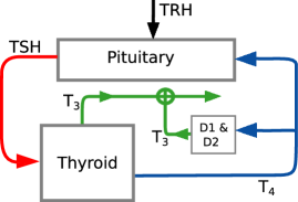
Figure 1: Simplified block diagram of the pituitary-thyroid feedback loop

One of the most important diseases related to the pituitary-thyroid feedback loop is Graves’ disease, in which autoimmune antibodies (more specifically thyrotropin receptor antibodies) overstimulate the production of thyroid hormones at the thyroid gland. Consequently, the hormone concentrations of $T_{3}$ and $T_{4}$ increase and the concentration of $TSH$ declines - a condition called hyperthyroidism. Several options exist to treat hyperthyroidism: First, one can surgically remove (parts of) the thyroid gland, called thyroidectomy, which, on one side, leads almost always to hypothyroidism (denoting a lack of thyroid hormones) and, on the other side, goes along with the usual risks of a surgery. Second, one can destroy thyroid tissue with radioactive iodine, which, on the one hand, exposes patients to radioactive radiation and, on the other hand, also leads (in many cases) to hypothyroidism. Third, one can inhibit the (over-)production of thyroid hormones by antithyroid agents such as methimazole (MMI) (sometimes also referred to as thiamazole). This option is usually the first choice of physicians treating hyperthyroidism in Europe, since it does not go along with lifelong hypothyroidism as thyroidectomy and does not expose the body to radioactive radiation (Ross et al. (2016)). Therefore, a success of the approach based on antithyroid agents is crucial. However, finding accurate dosages for patients is challenging. There currently exist only guidelines for physicians how to determine the dosages, compare Ross et al. (2016); Lemmer and Brune (2007). This prescription typically goes along in a trial-and-error fashion, meaning that the physician prescribes an initial dosage and evaluates whether this dosage normalizes the hormone concentrations and reduces the symptoms. If this is not the case, the physician adapts the dosage (possibly several times). On the one hand, if the prescribed dosage is too low, the patient continuously suffers from hyperthyroid symptoms. On the other hand, if the prescribed dosage is inappropriately high, the patient suffers from symptoms of hypothyroidism and unnecessary side effects.

An appealing alternative to improve this suboptimal trial-and-error approach is a prescription of MMI using model-based control. Recently, Theiler-Schwetz et al. (2022) proposed to determine the dosages of MMI by means of a simple mathematical model of the pituitary-thyroid feedback loop and a PI controller. However, Theiler-Schwetz et al. (2022) consider an “intravenous” infusion of MMI for Graves’ disease patients, which is rarely the case in clinical practice. Furthermore, no analysis is done for hyperthyroid patients affected by high intrathyroidal iodide concentrations, which typically occurs when iodinated contrast media are given for radiographic procedures. In the dual context of finding optimal medication strategies for hypothyroid patients, various different model-based approaches are available, compare, e.g., the works of Cruz-Loya et al. (2022); Wolff et al. (2022a); Brun et al. (2021).

In this paper, we develop optimal prescription policies for hyperthyroid patients. To this end, we extend a mathematical model of the pituitary-thyroid feedback loop developed in Dietrich (2001); Berberich et al. (2018); Wolff et al. (2022b) to allow an intravenous and an oral intake of antithyroid agents. Furthermore, we design a model predictive control (MPC) scheme to determine optimal dosages in case of (i) patients affected by Graves’ disease, which take in MMI orally once a day, (ii) patients that are additionally affected by high intrathyroidal iodide concentrations due to radiographic procedures (taking MMI also orally once a day) and, (iii) patients suffering from a life-threatening thyrotoxicosis (denoting a substantial excess of thyroid hormones that is associated with weight loss, atrial fibrillation, and, rarely, death (Ross et al., 2016)), in which MMI is given intravenously three times per day.

This approach leads to the following contributions. Our simulation results suggest that the MPC scheme is well suited to replace the current trial-and-error approach in the three mentioned scenarios. Furthermore, our results give additional evidence to the current treatment guidelines of prescribing higher MMI dosages in case of an increased intrathyroidal iodide concentration and of prescribing further medications (than just MMI) in case of a life-threatening thyrotoxicosis.

2 Model Extensions & Controller Design

The differential equations of the entire mathematical model can be found in Appendix A and a detailed explanation regarding their meaning in the Supplementary Material of Wolff et al. (2022b) and in Degon et al. (2008). The numerical parameter values of equations (10) - (15) and of equations (19) - (21) are given in the Supplementary Material of Wolff et al. (2022a), whereas the numerical parameter values of equation (16) and of equations (22) - (25) are documented in Degon et al. (2008) and in Degon et al. (2005). These parameter values represent a generic healthy individual. Here, we extend this model such that the main mechanism of MMI is considered, namely the intrathyroidal inhibition of the activity of thyroid peroxidase (TPO), which is a crucial enzyme for the synthesis of $T_{3}$ and $T_{4}$ in the thyroid gland. Precisely, TPO catalyzes the iodination (denoting an incorporation of iodine atoms into a molecule) of tyrosyl residues on thyroglobulin (a precursor protein of the thyroid hormones), compare Manna et al. (2013) for a detailed explanation of TPO’s mechanism.

To model this mechanism, we first consider the relationship between MMI that is taken in orally (once at some time $t_{0}$) and its subsequent plasma concentration by means of a Bateman function (compare, e.g., Garrett (1994))

$$MMI_{\mathrm{Pl}}(t)=\frac{fu(t_{0})k_{a}}{V(k_{a}-k_{e})}\big{(}e^{-k_{e}(t-t_{0})}-e^{-k_{a}(t-t_{0})}\big{)},$$ (1)

where $MMI_{\mathrm{Pl}}(t)$ denotes the concentration of MMI in the plasma at time $t$, $f$ the bioavailability of MMI, $u(t_{0})$ the dosage of MMI at time $t_{0}$, $V$ the volume of distribution, $k_{e}$ the elimination constant, and $k_{a}$ the absorption constant. Numerical values for these parameters are available in the literature or calculated according to data available in the literature. Precisely, we consider $f=0.93$ (Jansson et al. (1985)), $V=$28.8\text{\,}\mathrm{L}$$ (Melander et al. (1980)), $k_{e}=$0.1857\text{\,}\frac{1}{\mathrm{h}}$$ (Melander et al. (1980)), and $k_{a}=$11\text{\,}\frac{1}{\mathrm{h}}$$ (Melander et al. (1980)). The dosage $u(t_{0})$ is determined by the controller.

Second, we model (heuristically, i.e., after having tested different transfer functions) the relation between the MMI concentration in the plasma and the intrathyroidal MMI concentration, denoted by $MMI_{\mathrm{th}}$, as a linear transfer function with two poles and one zero (also known as $PDT_{2}$ element)

$$G(s)=\frac{b_{1}s+b_{0}}{s^{2}+a_{1}s+a_{0}}.$$ (2)

The parameter estimation is done by means of data available in Marchant and Alexander (1972). In this study, radioactively marked MMI was injected into rats. Then, at different time points, the radioactivity in the thyroid gland (and in other tissues) was measured. These input-output data allow to parameterize the transfer function by applying Matlab’s system identification toolbox (which is based on the Levenberg-Marquardt method), see Ljung (1988). The numerical values of the estimated parameters are $b_{1}=690.3\cdot 10^{-6}$, $b_{0}=37\cdot 10^{-9}$, $a_{1}=92.2\cdot 10^{-6}$, and $a_{0}=2.5\cdot 10^{-9}$.

Third, we establish a relation between the intrathyroidal MMI concentration and the inhibition of the activity of TPO. To this end, we exploit the results of Taurog (1976), which are based on a model incubation system. As illustrated by the different curves in Figure 9 of Taurog (1976), this relation depends on the concentration of inorganic iodide. The concentration of inorganic iodide in the thyroid is approximately $10^{-5}\>$\mathrm{mol}\mathrm{/}\mathrm{L}$$, based on the numerical values given in Degon et al. (2005). Then, we (heuristically) choose

$$TPO_{\mathrm{a}}(t)=c_{0}\big{(}1+\exp(-c_{1}(-MMI_{th}(t)^{1/c_{2}}+c_{3}))\big{)}^{-1}$$ (3)

to model the relation between the intrathyroidal MMI concentration and the activity of TPO. We estimate the parameters $c_{0}$, $c_{1}$, $c_{2}$, and $c_{3}$ by fitting (3) to the curve from Figure 9 of Taurog (1976) representing an iodide concentration of $10^{-5}\>$\mathrm{mol}\mathrm{/}\mathrm{L}$$, which is done by using the nonlinear regression tool $fitnlm$ from Matlab, which is once again based on the Levenberg-Marquardt method. The determined numerical parameter values are $c_{0}=0.9$, $c_{1}=84.1\cdot 10^{3}$, $c_{2}=1.3$, and $c_{3}=80.5\cdot 10^{-6}$.

Finally, we consider the iodide content in thyroglobulin by means of equation (16), which was originally developed in Degon et al. (2008). On the one hand, this content influences the synthesis of $T_{4,th}$, i.e., the first term of equation (10). On the other hand, it depends explicitly on the concentration of TPO. In other words, once the intrathyroidal MMI concentration reduces the activity of TPO, the concentration of $I_{Tg}$ decreases, which inhibits the production of $T_{4,th}$ and consequently of $T_{4}$ (and $T_{3}$).

Based on these model extensions, we implement an MPC scheme (Rawlings et al., 2020). Loosely speaking, the principle of MPC is the following. At each sampling instant $t=k\delta,\>k\in\mathbb{N}_{0}$, we measure the system’s state $x(t)$ and solve an optimal control problem to find the optimal input (i.e., MMI dosage) sequence with respect to a cost function over some control horizon $T$, which is an integer multiple of the sampling time $\delta$. Next, we apply only the first element of the optimal input sequence to the system. Finally, the system’s state is measured again and the whole process is repeated. The here applied setting for nonlinear systems in continuous time is as follows: At each sampling instant $t$, solve

$$\min_{\bar{u}_{t}}J\big{(}x(t),\bar{u}_{t}\big{)}$$ (4)

with

$$J(x(t),\bar{u}_{t})= \int_{t}^{t+T}||\bar{x}(\tau;t)-x_{s}||_{Q}^{2}d\tau$$

$$+ \sum_{k=0}^{T/\delta-1}||\bar{u}(t+k\delta;t)||_{R_{1}}^{2}$$

$$+||\bar{u}(t+k\delta;t)-\bar{u}^{\ast}(t-\delta;t-\delta)||_{R_{2}}^{2},$$ (5)

subject to the constraints

$$\dot{\bar{x}}(\tau;t)=f(\bar{x}(\tau;t),\bar{u}(\tau;t)),\quad\bar{x}(t;t)=x(t),\quad\bar{u}_{t}\in\mathcal{U}^{T/\delta}$$

for $\tau\in[t,t+T]$ and $\bar{u}_{t}:=\{\bar{u}(t;t),\bar{u}(t+\delta;t),\dots,\bar{u}(t+T-\delta;t)\}$, which is the optimization variable. Note that we only optimize over the input $\bar{u}$ at the discrete time points $t+k\delta$, since the medication is typically taken in orally, i.e., at discrete time points. The input $\bar{u}$ for all time instants is given by

$$\bar{u}(\tau;t):=\sum_{k=0}^{T/\delta-1}\bar{u}(t+k\delta;t)\delta_{\mathrm{Di}}(\tau-(t+k\delta)),$$ (6)

which means that the input is zero except for the sampling instants $t+k\delta$, as described by the Dirac-delta impulse $\delta_{\mathrm{Di}}$. In (5), $J$ denotes the cost functional to be minimized. The notations $\bar{x}(\tau;t)$ and $\bar{u}(\tau;t)$ stand for the predicted state $\bar{x}$ and the predicted input $\bar{u}$ at time $\tau$, predicted at time $t$, respectively, and $\bar{u}^{*}(\cdot;t)$ and $\bar{x}^{*}(\cdot;t)$ denote the optimal predicted trajectories. The setpoint $x_{s}$ corresponds to the steady-state hormone concentrations of healthy individuals. The closed-loop input, i.e., the input that is applied to the system, is defined as $u(t)\coloneqq\bar{u}^{\ast}(t;t)$. In the cost function, besides the standard input penalty (with weight $R_{1}$), we include a term (with weight $R_{2}$) that penalizes the difference of the predicted input trajectory to the previously optimal input (i.e., dosage) $u(t-\delta)=\bar{u}^{*}(t-\delta;t-\delta)$ in order to keep the same dosage as long as possible to avoid frequent (and uncomfortable) dosage adaptations for the patients. The weighing matrix $Q$ penalizes the difference between the predicted $T_{4}$, $T_{3}$, and $TSH$ concentrations to the setpoint, which corresponds to the healthy steady-state concentrations. The system dynamics $f(x,u)$ correspond to the right-hand sides of equations (10) - (18). The input constraint set is defined as

$$\mathcal{U}\coloneqq\{u\in\mathbb{R}|\>0\leq u\leq u_{\mathrm{max}}\},$$ (7)

since the input, i.e., the dosage of MMI, must be limited to avoid the prescription of inadequately high dosages. Precisely, $u_{\mathrm{max}}$ is set to $15\text{\,}\mathrm{mg}$ in Subsection 3.1, to $35\text{\,}\mathrm{mg}$ in Subsection 3.2, and to $40\text{\,}\mathrm{mg}$ in Subsection 3.3. Since, e.g., in case of a life-threatening thyrotoxicosis (which is considered in Subsection 3.3), the primary objective is to bring the hormone concentration into a normal range as fast as possible, higher maximal dosages are allowed. The control horizon $T$ is set to 10 days. Furthermore, the sampling time $\delta$ is chosen as $24\>$\mathrm{h}$$ and $8\>$\mathrm{h}$$ in Subsections 3.1, 3.2, and in Subsection 3.3, respectively. Finally, the cost function’s weighting matrices $Q$, $R_{1}$, and $R_{2}$ are chosen as

$$Q=\begin{bmatrix}0&0&0&0&0&0&0&0\\ 0&10^{3}&0&0&0&0&0&0\\ 0&0&10^{3}&0&0&0&0&0\\ 0&0&0&0&0&0&0&0\\ 0&0&0&0&10^{3}&0&0&0\\ 0&0&0&0&0&0&0&0\\ 0&0&0&0&0&0&0&0\\ 0&0&0&0&0&0&0&0\\ \end{bmatrix},R_{1}=5\cdot 10^{-3},R_{2}=10^{-2}.$$

As mentioned above, the MPC formulation (4) is non-standard since the input is not applied continuously, but only at discrete time instants (one or three times per day). Moreover, the inputs applied at previous sampling instants influence the dynamics at the current and future sampling instants (since the medication of, e.g., the previous day is not completely absorbed and still affects the production of thyroid hormones at the current day and the future days). Precisely, when implementing the MPC scheme, instead of (1), which describes a single medication intake, at prediction time $t+k\delta$, we need to consider

$$MMI_{Pl}(t+k\delta;t)=\frac{fk_{a}}{V(k_{a}-k_{e})}$$

$$\times\Bigg{(}\sum_{\ell=0}^{t/\delta-1}u(\ell)(e^{-k_{e}(t+(k-\ell)\delta)}-e^{-k_{a}(t+(k-\ell)\delta)})$$

$$+\sum_{i=t/\delta}^{t/\delta+k-1}\bar{u}(i\delta;t)(e^{-k_{e}(t+(k-i)\delta)}-e^{-k_{a}(t+(k-i)\delta)})\Bigg{)},$$ (8)

which denotes the predicted concentration of MMI in the plasma at time $t+k\delta$, predicted at time $t$. In particular, we need to consider (i) the medication that has already been taken in, which is not completely absorbed (first sum), and (ii) the medication that shall be taken in over the horizon, where the different dosages are considered as optimization variables (second sum). The MPC scheme is implemented in CasADi (Andersson et al., 2019) applying the single-shooting method. To obtain the discretized dynamics, we employ the cvodes integrator from the SUNDIALS suite (Hindmarsh et al., 2005) instead of the typical fixed step Runge-Kutta 4 integrator, since the considered system reveals stiff dynamics.

3 Simulation Results

In the following simulations, we consider a sinusoidal $TRH$ concentration as an approximation of the real pulsatile $TRH$ course. Furthermore, at the beginning of the simulations in Subsections 3.1 and 3.2, the hormone concentrations are set to their hyperthyroid steady states, which are deduced by considering a 10-fold (15-fold in Subsection 3.3) increase in the secretory capacity of the thyroid gland, named $G_{T}$. The setpoints, illustrated by the dashed lines in Figures 2, 3, and 4, correspond to the steady-state hormone concentrations of healthy individuals. Moreover, at the beginning of the simulations, we set $\bar{u}^{\ast}(t-\delta;t-\delta)=u_{\mathrm{max}}$ to incentivize the prescription of high initial dosages.

In each subsection, we execute two different simulations. First, we consider a nominal case (illustrated in Figures 2, 3, and 4 by the dotted lines), in which no measurement noise, no model-plant mismatch, or other types of disturbances affect the system. Second, we consider a more realistic scenario (illustrated in Figures 2, 3, and 4 by the continuous lines), in which the state measurements are corrupted by some measurement noise $v\sim\mathcal{N}(0,0.05^{2})$ (truncated at $\pm 0.3$ to avoid negative hormone concentrations after adding the measurement noise). Furthermore, we consider exemplarily a model-plant mismatch by increasing the numerical values of the parameters $G_{D1}$ and $G_{T3}$ (describing the maximum activity of D1 and the maximum activity of the direct $T_{3}$ synthesis, respectively) by 10 % in the model that is used to simulate the measurements, but, obviously, not in the prediction model used by the MPC scheme. Finally, we consider that the patient forgets to take in her/his daily dosage at days 4 and 14. In Subsection 3.3, we do not consider that any medication is forgotten to be taken in, since in a life-threatening thyrotoxicosis, the administration of the medication is monitored by nurses or physicians.

3.1 Ordinary Treatment

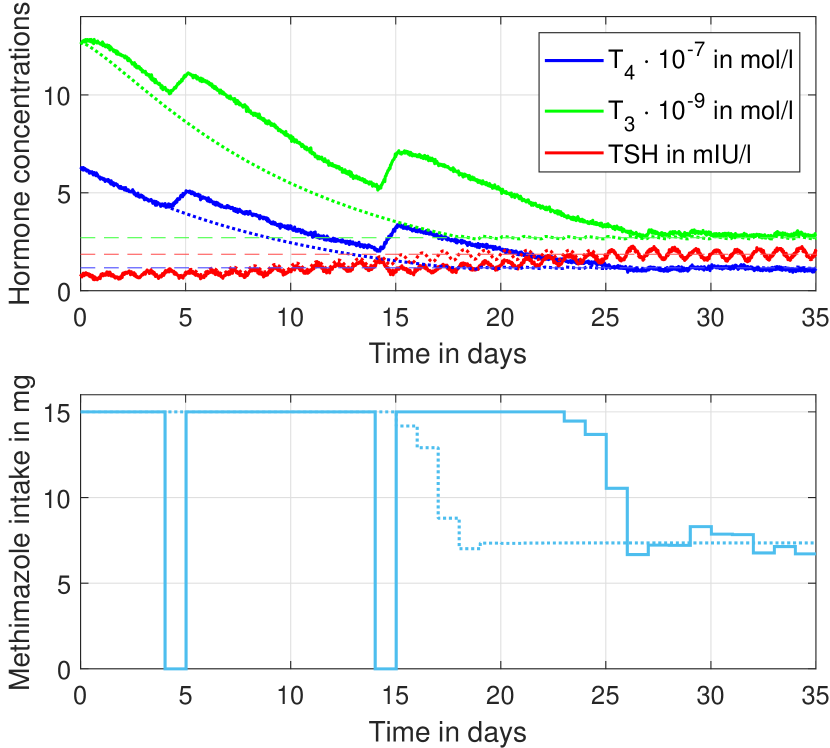
Figure 2: Course of the hormone concentrations and the corresponding dosages of MMI for hyperthyroid patients and one daily oral MMI intake. The daily dosages are determined by means of the MPC scheme. The dotted lines represent the treatment without any kind of disturbances. The continuous lines illustrate the treatment in case of measurement noise, a model-plant mismatch, and two forgotten dosages, namely at days 4 and 14.

Here, we consider typical hyperthyroid patients affected by Graves’ disease which take in MMI orally once a day. We illustrate the results of our approach in Figure 2. In both cases, the determined MMI dosages are in line with clinical guidelines, suggesting an initial dosage of $10-40\>$\mathrm{mg}$$ per day and, as maintenance dosage, $5-10\>$\mathrm{mg}$$ per day (Ross et al., 2016; Lemmer and Brune, 2007). In the nominal case, the hormone concentrations reach the setpoint already after 17 days. In contrast, in the more realistic scenario, the hormone concentrations reach the setpoint after 26 days, which is mainly due to the forgotten dosages. The measurement noise and the model-plant mismatch lead to fluctuations in the prescribed MMI dosages, especially after day 25.

3.2 Increased Intrathyroidal Iodide Concentration

In this subsection, we consider hyperthyroid patients that have additionally increased intrathyroidal iodide concentrations, which typically come from radiographic procedures dealing with iodinated contrast media (Bervini et al., 2021). Higher iodide concentrations can easily be considered in the mathematical model. We here consider exemplarily a 10-fold increase in the iodide concentration, i.e., $10^{-4}\>$\mathrm{mol}\mathrm{/}\mathrm{L}$$, and subsequently re-estimate the parameters of equation (3) describing the effects of the intrathyroidal MMI concentration on the activity of TPO, which results in $c_{0}=1$, $c_{1}=175.8\cdot 10^{3}$, $c_{2}=5$, and $c_{3}=97.6\cdot 10^{-3}$. The optimal dosages are determined by means of the MPC scheme and shown in Figure 3. In the nominal case and in the more realistic case, the required dosages to normalize the hormone concentrations are approximately two times higher and the dosages to remain in the steady state are approximately three times higher compared to the hyperthyroid patients considered in Figure 2. It is well known that patients with high intrathyroidal iodide concentrations need higher MMI dosages, e.g., Lemmer and Brune (2007) suggest as initial dosage $20-40\>$\mathrm{mg}$$ of MMI. Therefore, our results support the current clinical guidelines to prescribe higher dosages of MMI in case of increased intrathyroidal iodide concentrations. Once again, the forgotten dosages substantially prolongs the time (by approximately 10 days) until the steady state is reached. The measurement noise and the exemplary model-plant mismatch lead to MMI dosages that fluctuate substantially more compared to the nominal case.

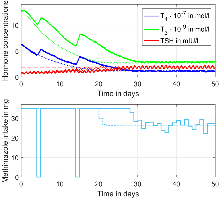
Figure 3: Course of the hormone concentrations and the corresponding dosages of MMI for hyperthyroid patients affected by high intrathyroidal iodide concentrations. The dotted lines represent the treatment, when no disturbances affect the system. The continuous lines represent the treatment in case of measurement noise, a model-plant mismatch, and forgotten dosages.

3.3 Life-Threatening Thyrotoxicosis

Finally, we consider patients suffering from a life-threatening thyrotoxicosis that are treated by means of intravenous MMI boluses that are injected three times per day. Therefore, in contrast to equation (1), we here model the intravenous intake of MMI (given once at some time $t_{0}$) as

$$MMI_{\mathrm{Pl}}(t)=\frac{u(t_{0})}{V}e^{-k_{e}(t-t_{0})},$$ (9)

meaning that all of the given MMI is absorbed and directly available in the plasma. The corresponding results are illustrated in Figure 4. In this figure, one can see that it takes approximately 21 days to restore normal hormone concentrations in the nominal case. This rather long time is due to the following. On the one hand, the hormone concentrations of $T_{4}$ and $T_{3}$ are very high and the concentration of $TSH$ is very low (since we consider a 15-fold increase of the secretory capacity of the thyroid gland). On the other hand, the decrease of the hormone concentration only comes from the endogenous metabolism. The hormone $T_{4}$ has a half-life of approximately one week, meaning that 12.5 % of the concentration at the beginning of the simulation remains after three weeks. This behavior can clearly be observed in Figure 4, in which the concentration of $T_{4}$ starts at approximately $8\cdot 10^{-7}\>$\mathrm{mol}\mathrm{/}\mathrm{L}$$ and corresponds approximately to $1\cdot 10^{-7}\>$\mathrm{mol}\mathrm{/}\mathrm{L}$$ after three weeks. In addition, one can observe the effect of the model-plant mismatch: The increased $G_{D1}$ and $G_{T3}$ parameters lead to slightly higher $T_{3}$ (and slightly lower $T_{4}$) concentrations in the more realistic case compared to the nominal case. In general, the results underline the importance to prescribe further medication (usually medication that inhibits the release of thyroid hormones such as, e.g., lithium and/or medication that inhibits the thyroid hormones’ enterohepatic circulation to reduce their half-lives such as, e.g., colestyramine (Dietrich, 2012)) to normalize the hormone concentrations as fast as possible.

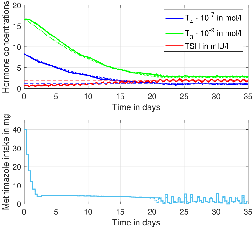
Figure 4: Course of the hormone concentrations and the corresponding dosages of MMI that are given intravenously three times per day. The dotted lines represent the treatment, when no disturbances affect the dynamics and the continuous lines represent the treatment in case of measurement noise and a model-plant mismatch.

4 Conclusion & Discussion

This paper presents an approach to treat hyperthyroidism using model-based control. Based on an extension of a mathematical model of the pituitary-thyroid feedback loop and on an MPC scheme, we determine optimal MMI dosages for hyperthyroid patients. We illustrate the performance of the MPC scheme in case of (i) an ordinary treatment of hyperthyroidism, (ii) additional high intrathyroidal iodide concentrations, and (iii) a life-threatening thyrotoxicosis. The results suggest that the prescription of MMI based on an MPC scheme is a promising alternative compared to the traditional trial-and-error approach.

Various challenges remain to translate these results into clinical practice. First, the current implementation requires one measurement per day (or three measurements per day), which is typically not the case in clinical practice, where measurements are taken every 2 - 6 weeks (Ross et al., 2016). These rather long sampling intervals are justified by the long half-life of $T_{4}$. In thyroid emergencies, the interval between blood sampling may be shorter, but usually sampling frequencies would not exceed one to two measurements per week. To alleviate this issue, one could implement a multi-step MPC algorithm meaning that one applies multiple steps of the optimal input trajectory. In this case, one might need to extend (considerably) the horizon of the MPC algorithm. Second, we currently assume that all states are measurable (full-state feedback), which is not the case in clinical practice, where only the concentrations of $T_{4}$, $T_{3}$, and $TSH$ can be measured. This implies that the states would need to be reconstructed by applying some (reduced-order) observer. Third, in most cases, the measurements of the hormone concentrations are not available instantaneously. Usually, the blood samples taken from patients are sent to a laboratory. Once the measurements are finished, the results are sent back to the treating physician. This substantial time-delay would also need to be incorporated into the prediction, potentially by means of an observer which is capable of dealing with time-delays.

Appendix A System Dynamics

The system’s differential equations are

$$\frac{dT_{4,th}}{dt}(t)=\alpha_{th}\Bigg{(}\frac{G_{T}TSH(t)}{TSH(t)+D_{T}}K_{I}I_{T_{g}}(t)$$

$$\hskip 14.22636pt-G_{MCT8}\frac{T_{4,th}(t)}{K_{MCT8}+T_{4,th}(t)}$$

$$\hskip 14.22636pt-G_{D1}\frac{T_{4,th}(t)\frac{TSH(t)}{TSH(t)+k_{Dio}}}{T_{4,th(t)}\frac{TSH(t)}{TSH(t)+k_{Dio}}+K_{M1}}$$

$$\hskip 14.22636pt-G_{D2}\frac{T_{4,th}(t)\frac{TSH(t)}{TSH(t)+k_{Dio}}}{T_{4,th}(t)\frac{TSH(t)}{TSH(t)+k_{Dio}}+K_{M2}}\Bigg{)}-\beta_{th}T_{4,th}(t)$$ (10)

$$\frac{dT_{4}}{dt}(t)=\alpha_{T}G_{MCT8}\frac{T_{4,th}(t)}{K_{MCT8}+T_{4,th}(t)}-\beta_{T}T_{4}(t)$$ (11)

$$\frac{dT_{3}}{dt}(t)=\alpha_{31}\Bigg{(}G_{D1}\frac{FT_{4}(t)}{FT_{4}(t)+K_{M1}}+G_{D2}\frac{FT_{4}(t)}{FT_{4}(t)+K_{M2}}$$

$$\hskip 14.22636pt+\frac{G_{D1}T_{4,th}(t)\frac{TSH(t)}{TSH(t)+k_{Dio}}}{T_{4,th}(t)\frac{TSH(t)}{TSH(t)+k_{Dio}}+K_{M1}}$$

$$\hskip 14.22636pt+\frac{G_{D2}T_{4,th}(t)\frac{TSH(t)}{TSH(t)+k_{Dio}}}{T_{4,th}(t)\frac{TSH(t)}{TSH(t)+k_{Dio}}+K_{M2}}$$

$$\hskip 14.22636pt+G_{T3}\frac{TSH(t)}{D_{T}+TSH(t)}\Bigg{)}-\beta_{31}T_{3}(t)$$ (12)

$$\frac{dT_{3c}}{dt}(t)=\alpha_{32}G_{D2}\frac{FT_{4}(t)}{FT_{4}(t)+K_{M2}}-\beta_{32}T_{3c}(t)$$ (13)

$$\frac{dTSH}{dt}(t)=\frac{\alpha_{S}G_{H}TRH(1+0.3\cos(2\pi(t/86400-5/24)))}{(TRH(1+0.3\cos(2\pi(t/86400-5/24)))+D_{H})}$$

$$\hskip 14.22636pt\times\frac{1}{(1+S_{S}\frac{TSH_{z}(t)}{TSH_{z}(t)+D_{S}})(1+L_{S}G_{R}\frac{T_{3N}(t)}{T_{3N}(t)+D_{R}})}$$

$$\hskip 14.22636pt-\beta_{S}TSH(t)$$ (14)

$$\frac{dTSH_{z}}{dt}(t)=\frac{\alpha_{S2}G_{H}TRH(1+0.3\cos(2\pi(t/86400-5/24)))}{(TRH(1+0.3\cos(2\pi(t/86400-5/24)))+D_{H})}$$

$$\hskip 14.22636pt\times\frac{1}{(1+S_{S}\frac{TSH_{z}(t)}{TSH_{z}(t)+D_{S}})(1+L_{S}G_{R}\frac{T_{3N}(t)}{T_{3N}(t)+D_{R}})}$$

$$\hskip 14.22636pt-\beta_{S2}TSH_{z}(t)$$ (15)

$$\frac{dI_{Tg}}{dt}(t)=\frac{\tau^{TPO}_{\mathrm{turnover}}TPO(t)TPO_{\mathrm{a}}(t)V_{org}^{H_{2}O_{2}}H_{2}O_{2}}{K_{org}^{H_{2}O_{2}}+H_{2}O_{2}}$$

$$\hskip 14.22636pt\times\frac{V_{org}^{I_{C}}I_{C}V_{org}^{T_{g,\mathrm{eff}}}T_{g,\mathrm{eff}}(t)}{(K_{org}^{I_{C}}+I_{C})(K_{org}^{T_{g,\mathrm{eff}}}+T_{g,\mathrm{eff}}(t))}$$

$$\hskip 14.22636pt-\frac{V_{\mathrm{apical}}^{SSF}SSF(t)A_{\mathrm{apical}}\alpha_{\mathrm{endo}}I_{T_{g}}(t)}{(K_{\mathrm{apical}}^{SSF}+SSF(t))A_{\mathrm{apical,nom}}}$$ (16)

$$\frac{dMMI_{1}}{dt}(t)=MMI_{2}(t)$$ (17)

$$\frac{dMMI_{2}}{dt}(t)=-a_{0}MMI_{1}(t)-a_{1}MMI_{2}(t)+MMI_{\mathrm{Pl}}(t)$$ (18)

with the relationships

$$FT_{3}(t) =T_{3p}(t)\frac{1}{1+K_{30}TBG}$$ (19)

$$FT_{4}(t) =T_{4}(t)\frac{1}{1+K_{41}TBG+K_{42}TBPA}$$ (20)

$$T_{3N}(t) =T_{3c}(t)\frac{1}{1+K_{31}IBS}$$ (21)

$$TPO(t) =\frac{V_{TPO}^{SSF}SSF(t)}{K_{TPO}^{SSF}+SSF(t)}\frac{V_{\mathrm{colloid,nom}}}{V_{\mathrm{colloid}}}\frac{\alpha_{TPO}^{T_{g}}}{K_{TPO}^{T_{g}}+T_{g}}\mathrm{scale}$$ (22)

$$SSF(t) =\frac{100TSH(t)-R\cdot TSH(t)}{178.2+TSH(t)}$$ (23)

$$T_{g,\mathrm{eff}}(t) =\Big{(}1-\frac{I_{T_{g}}(t)}{T_{g}}\Big{)}$$ (24)

$$\mathrm{scale} =\frac{V_{\mathrm{measured}}-0.17(1.97+0.21\mathrm{weight}+0.06\mathrm{age})}{1.97+0.21\mathrm{weight}+0.06\mathrm{age}}$$ (25)

$$MMI_{\mathrm{th}}(t) =b_{0}MMI_{1}(t)+b_{1}MMI_{2}(t).$$ (26)

References

- Andersson et al. (2019) Andersson, J.A.E., Gillis, J., Horn, G., Rawlings, J.B., and Diehl, M. (2019). CasADi – A software framework for nonlinear optimization and optimal control. Mathematical Programming Computation, 11(1), 1–36.
- Berberich et al. (2018) Berberich, J., Dietrich, J.W., Hoermann, R., and Müller, M.A. (2018). Mathematical modeling of the pituitary-thyroid feedback loop: role of a TSH-T3-Shunt and sensitivity analysis. Frontiers in Endocrinology, 9(91).
- Bervini et al. (2021) Bervini, S., Trelle, S., Kopp, P., Stettler, C., and Trepp, R. (2021). Prevalence of iodine-induced hyperthyroidism after administration of iodinated contrast during radiographic procedures: a systematic review and meta-analysis of the literature. Thyroid, 31(7), 1020–1029.
- Brun et al. (2021) Brun, V.H., Eriksen, A.H., Selseth, R., Johansson, K., Vik, R., Davidsen, B., Kaut, M., and Hellemo, L. (2021). Patient-tailored levothyroxine dosage with pharmacokinetic/pharmacodynamic modeling: a novel approach after total thyroidectomy. Thyroid, 31(9), 1297–1304.
- Cruz-Loya et al. (2022) Cruz-Loya, M., Chu, B.B., Jonklaas, J., Schneider, D.F., and DiStefano, J. (2022). Optimized replacement T4 and T4+T3 dosing in male and female hypothyroid patients with different BMIs using a personalized mechanistic model of thyroid hormone regulation dynamics. Frontiers in Endocrinology, 13(888429).
- Degon et al. (2005) Degon, M., Chait, Y., Hollot, C., Chipkin, S., and Zoeller, T. (2005). A quantitative model of the human thyroid: development and observations. In Proceedings of the 2005, American Control Conference, 961–966.
- Degon et al. (2008) Degon, M., Chipkin, S.R., Hollot, C.V., Zoeller, R.T., and Chait, Y. (2008). A computational model of the human thyroid. Mathematical biosciences, 212, 22–53.
- Dietrich (2001) Dietrich, J.W. (2001). Der Hypophysen-Schilddrüsen-Regelkreis: Entwicklung und klinische Anwendung eines nichtlinearen Modells. Ph.D. thesis.
- Dietrich (2012) Dietrich, J. (2012). Thyreotoxische Krise. Medizinische Klinik-Intensivmedizin und Notfallmedizin, 107(6), 448–453.
- Garrett (1994) Garrett, E.R. (1994). The Bateman function revisited: a critical reevaluation of the quantitative expressions to characterize concentrations in the one compartment body model as a function of time with first-order invasion and first-order elimination. Journal of Pharmacokinetics and Biopharmaceutics, 22(2), 103–128.
- Hindmarsh et al. (2005) Hindmarsh, A.C., Brown, P.N., Grant, K.E., Lee, S.L., Serban, R., Shumaker, D.E., and Woodward, C.S. (2005). SUNDIALS: Suite of nonlinear and differential/algebraic equation solvers. ACM Transactions on Mathematical Software (TOMS), 31(3), 363–396.
- Jansson et al. (1985) Jansson, R., Lindström, B., and Dahlberg, P. (1985). Pharmacokinetic properties and bioavailability of methimazole. Clinical Pharmacokinetics, 10(5), 443–450.
- Lemmer and Brune (2007) Lemmer, B. and Brune, K. (2007). Pharmakotherapie: Klinische Pharmakologie. Springer Berlin, Heidelberg.
- Ljung (1988) Ljung, L. (1988). System identification toolbox. The Matlab user’s guide.
- Manna et al. (2013) Manna, D., Roy, G., and Mugesh, G. (2013). Antithyroid drugs and their analogues: synthesis, structure, and mechanism of action. Accounts of Chemical Research, 46(11), 2706–2715.
- Marchant and Alexander (1972) Marchant, B. and Alexander, W. (1972). The thyroid accumulation, oxidation and metabolic fate of 35s—methimazole in the rat. Endocrinology, 91(3), 747–756.
- Melander et al. (1980) Melander, A., Hallengren, B., Rosendal-Helgesen, S., Sjöberg, A.K., and Wåhlin-Boll, E. (1980). Comparative in vitro effects and in vivo kinetics of antithyroid drugs. European Journal of Clinical Pharmacology, 17(4), 295–299.
- Rawlings et al. (2020) Rawlings, J.B., Mayne, D.Q., and Diehl, M. (2020). Model predictive control: theory, computation, and design. Nob Hill Publishing Madison, WI, 2 edition.
- Ross et al. (2016) Ross, D.S., Burch, H.B., Cooper, D.S., Greenlee, M.C., Laurberg, P., Maia, A.L., Rivkees, S.A., Samuels, M., Sosa, J.A., Stan, M.N., et al. (2016). 2016 American Thyroid Association guidelines for diagnosis and management of hyperthyroidism and other causes of thyrotoxicosis. Thyroid, 26(10), 1343–1421.
- Taurog (1976) Taurog, A. (1976). The mechanism of action of the Thioureylene antithyroid drugs. Endocrinology, 98(4), 1031–1046.
- Theiler-Schwetz et al. (2022) Theiler-Schwetz, V., Benninger, T., Trummer, C., Pilz, S., and Reichhartinger, M. (2022). Mathematical modeling of free thyroxine concentrations during methimazole treatment for Graves’ disease: development and validation of a computer-aided thyroid treatment method. Frontiers in Endocrinology, 13(841888).
- Wächter and Biegler (2006) Wächter, A. and Biegler, L.T. (2006). On the implementation of an interior-point filter line-search algorithm for large-scale nonlinear programming. Mathematical programming, 106(1), 25–57.
- Wolff et al. (2022a) Wolff, T.M., Dietrich, J.W., and Müller, M.A. (2022a). Optimal hormone replacement therapy in hypothyroidism - a model predictive control approach. Frontiers in Endocrinology, 13(884018).
- Wolff et al. (2022b) Wolff, T.M., Veil, C., Dietrich, J.W., and Müller, M.A. (2022b). Mathematical modeling of thyroid homeostasis: implications for the Allan-Herndon-Dudley Syndrome. bioRxiv, accepted for Frontiers in Endocrinology.