RFEPS: Reconstructing Feature-line Equipped Polygonal Surface

Abstract.

Feature lines are important geometric cues in characterizing the structure of a CAD model. Despite great progress in both explicit reconstruction and implicit reconstruction, it remains a challenging task to reconstruct a polygonal surface equipped with feature lines, especially when the input point cloud is noisy and lacks faithful normal vectors. In this paper, we develop a multistage algorithm, named RFEPS, to address this challenge. The key steps include (1) denoising the point cloud based on the assumption of local planarity, (2) identifying the feature-line zone by optimization of discrete optimal transport, (3) augmenting the point set so that sufficiently many additional points are generated on potential geometry edges, and (4) generating a polygonal surface that interpolates the augmented point set based on restricted power diagram. We demonstrate through extensive experiments that RFEPS, benefiting from the edge-point augmentation and the feature preserving explicit reconstruction, outperforms state of the art methods in terms of the reconstruction quality, especially in terms of the ability to reconstruct missing feature lines.

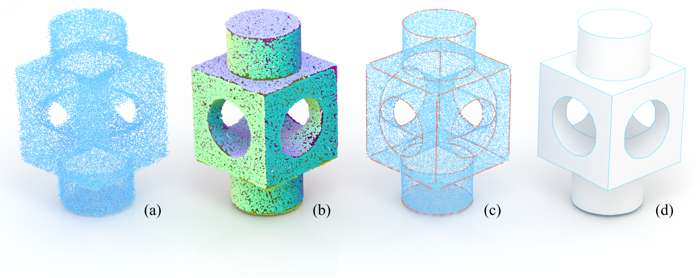
Figure 1. Reconstructing a polygonal surface with clean line-type features from a noisy point cloud. From left to right: (a) The input point cloud is noisy and does not have reliable normal information. (b) The point locations and normal vectors are optimized simultaneously such that the resulting point cloud is as locally planar as possible (the normal vectors of the denoised point cloud are visualized in a color-coded style). (c) We augment the point set by predicting more points that are deemed to be located on potential geometry edges; See the points colored in red. (d) Based on a power-diagram decomposition restricted on the base surface (obtained by Poisson reconstruction), the resulting polygonal surface interpolates the augmented point set and naturally aligns with feature lines.

1. Introduction

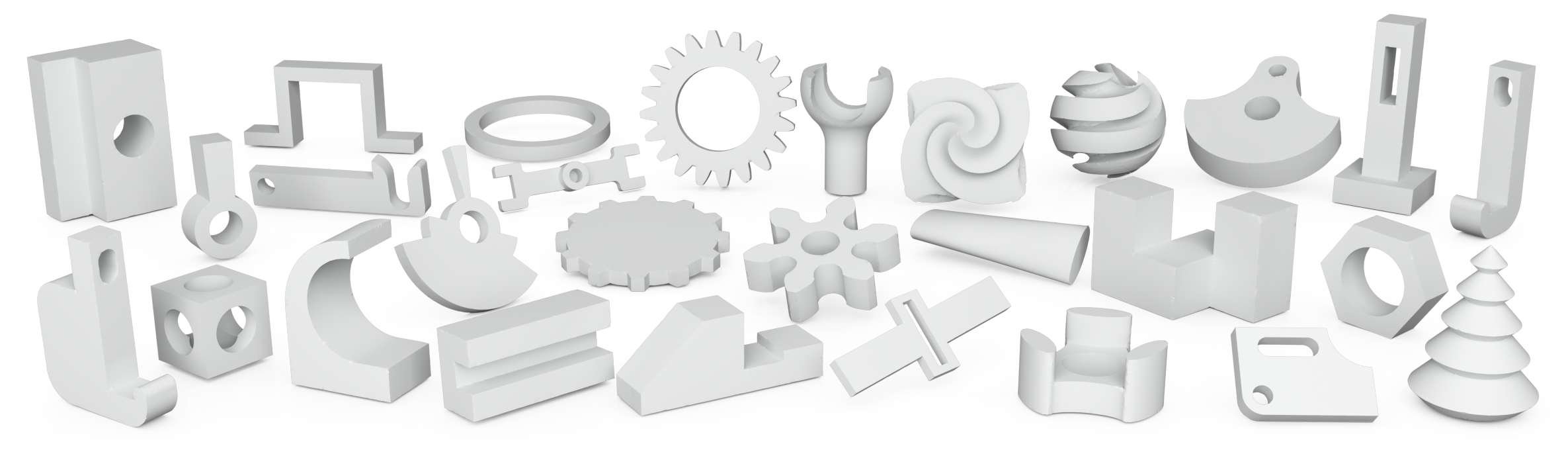
Figure 2. A gallery of reconstruction results by our RFEPS.

Inferring geometry from a low-quality point cloud belongs to the reverse engineering category, which is a fundamental problem in computer-aided design (Bénière et al., 2013; Willis et al., 2021; Birdal et al., 2019; Li et al., 2019; Sommer et al., 2020). Line-type features are critical geometric cues and can help characterize the structure of a CAD model, and thus serve as a base for a wide range of semantic manipulation tasks (Zhang et al., 2020; Wu and Kobbelt, 2005; Kós et al., 2000). In this paper, we take a noisy point cloud (the ground truth is a CAD model) without reliable normal vectors as the input and study how to recover a clean polygonal model exhibiting neat feature lines.

The challenges are two-fold. On the one hand, the general input point cloud contains few points that are precisely located on the underlying geometry edges. There are some point consolidation approaches (Yu et al., 2018; Huang et al., 2013; Cheng et al., 2019) that aim at increasing the point density in the edge zone, but the added points do not define feature lines of the target polygonal surface due to imprecise positions or insufficient density. There are also some approaches (Ma and Kruth, 1998; Dan and Lancheng, 2006; Naik and Jain, 1988) that separate the given points into a collection of patches, followed by fitting a smooth surface to each patch. However, it is hard to find the best decomposition that reveals the structure of the underlying CAD model. On the other hand, it is non-trivial to fully respect the line-type features during the mesh generation step. The existing explicit reconstruction approaches lack effective techniques to prioritize the connections between edge points.

In this paper, we introduce two separate techniques to deal with the above-mentioned difficulties. First, we observe that in the neighborhood of an edge point, the distribution of normal vectors can be represented as a combination of two independent sub-distributions with equal measure, and each sub-distribution is as simple as a Dirac delta function. Based on this observation, we formulate the identification of the edge zone as a discrete optimal mass transport problem, which can help regularize point locations and normal vectors, and predict the edge points as well. Second, we suggest using the restricted power diagram (RPD) to build connections between points. Compared with the restricted Voronoi diagram (RVD), the RPD not only has the nice feature of the RVD, but also allows to set a larger weight for edge points, thus encouraging edge points to naturally form feature lines with a higher priority than other points.

We propose a multistage algorithm named RFEPS to reconstruct a clean polygonal surface while manifesting the line-type features of CAD models. Our algorithm begins with a denoising step, which the point locations and the normal vectors are optimized simultaneously based on the assumption that a CAD-type point cloud tends to be locally planar; See Figure 1(b). Next, we generate sufficiently many additional points that are on potential geometry edges; See Figure 1(c). Finally, we run the Poisson reconstruction solver to get a base surface and then compute the restricted power diagram (RPD) to the base surface. The dual of the RPD reports a feature preserving polygonal mesh that interpolates the denoised and augmented point set; See Figure 1(d). Figure 2 shows a gallery of reconstruction results produced by our method. More tests on both synthetic and raw-scan data are provided in Section 4. We further demonstrate the utility of our approach in shape edit tasks; See Figure 21 in Section 4.9.

To summarize, our contributions are threefold:

1. We propose a multi-stage algorithm that transforms a noisy point cloud of a CAD model into a watertight manifold polygonal surface with neat feature lines.

2. We classify the points into nearby-edge points and off-edge points using a discrete optimal mass transport formulation, which enables us to generate sufficiently many additional points that are accurately located on potential geometry edges.

3. We set a larger weight for the newly added edge points and then use the restricted power diagram to reconstruct a polygonal surface that interpolates the augmented point set and aligns with the edges of the geometry.

2. Related Work

\begin{overpic}[width=429.28616pt]{pipeline1.png} \put(10.0,22.6){(a)} \put(36.0,22.6){(b)} \put(61.0,22.6){(c)} \put(86.0,22.6){(d)} \put(10.0,2.0){(h)} \put(36.0,2.0){(g)} \put(61.0,2.0){(f)} \put(86.0,2.0){(e)} \end{overpic}

Figure 3. The pipeline of the proposed method. (a) The noisy input point cloud. (b) The denoised result by optimizing point locations and normal vectors simultaneously. (c) The edge zone detected by a discrete optimal transport formulation. (d) The normal vectors of the points in the edge zone are regularized. (e) The point locations are fine-tuned to adapt to the regularized normal vectors. (f) Points in the edge zone are projected, point by point, onto the potential edge such that there are sufficiently many additional edge points (colored in red). (g) The restricted power diagram (RPD) on the base surface produced by the Poisson reconstruction solver. (h) The dual of the RPD reports the final reconstructed polygonal surface that interpolates the augmented point set while naturally aligning feature lines along geometry edges.

Point Cloud Consolidation

There has been a large body of literature on consolidating point clouds in the past decade. Most of them assume that the underlying surface is globally smooth. Alexa et al. (2001) suggested using moving least square (MLS) to increase or decrease the density of the points, allowing an adjustment of the spacing among the points. Lipman et al. (2007) presented a locally optimal projection operator (LOP) that provides a second-order approximation to the underlying smooth surface, thus facilitating resampling of the original point data. Huang et al. (2009) proposed a weighted LOP for denoising and outlier removal from imperfect point data, producing a set of evenly distributed particles that accurately adheres to the captured shape. However, the aforementioned approaches are weak in dealing with sharp features, which motivates researchers to consider line-type features on point-sampled geometry during point consolidation (Pauly et al., 2003; Guennebaud et al., 2004; Fleishman et al., 2005). Avron et al. (2010) defined an $l_{1}$-sparse optimization to denoise the input point cloud assuming that the target surface consists mainly of smooth patches, where the residual of the objective function is strongly concentrated near sharp features. Liao et al. (2013) took both spatial and geometric feature information into consideration for feature-preserving approximation. Huang et al. (2013) presented Edge-Aware Resampling (EAR) that re-samples the points away from the edges and then progressively fills the gap between the planes. Although the point density near the edges is increased, the added points are not precisely located on the edges. Lu et al. (2020) proposed a low-rank matrix approximation algorithm that can robustly estimate normals for both point clouds and meshes, which is helpful for edge-preserving upsampling. Recently, Chen et al. (2021) presented a two-phase algorithm for extracting line-type features from point clouds. But the accuracy of the predicted edge points is decreased if noise exists.

With the emergence of learning techniques, many data-driven approaches have been proposed to improve the robustness of edge detection and the preservation of sharp edges. To the best of our knowledge, EC-Net (Yu et al., 2018) is the first learnable edge-aware method that formulates a regression component to simultaneously recover 3D point coordinates and point-to-edge distances from upsampled features and an edge-aware joint loss function to directly minimize distances from output points to 3D meshes and edges. However, EC-Net cannot capture line-type features very precisely. Loizou et al. (2020) formulated the detection of sharp edges as a classification problem and adopted the extended EdgeConv (Wang et al., 2019) to accomplish this task. It has to leverage an additional post-processing step of Graph-Cut (Boykov et al., 2001) to generate reliable results. Wang et al. (2020a) suggested representing edges as a collection of parametric curves and proposed an end-to-end learnable technique to identify feature edges. PC2WF (Liu et al., 2021) introduced an end-to-end trainable deep network architecture to accomplish this challenging task, i.e., directly converting a 3D point cloud into a wireframe model. Nevertheless, the performance of these data-driven approaches could be influenced by the quantity, quality and relevance of the training dataset. Such approaches (Wang et al., 2020b) may produce promising results for a similar input but could be inadequate for different conditions (e.g., noise level).

Feature Preserving Surface Reconstruction

Sharp features need to be carefully handled in many geometry processing tasks. A typical situation is that the target surface may consist of smooth patches separated by feature lines (Huang and Ascher, 2008; Zhang et al., 2015; Shen et al., 2022), especially in the field of CAD. Owing to the piecewise shape representation, Du et al. (2021) proposed a representation of Boundary-Sampled Halfspaces (BSH). Therefore, it is necessary to preserve line-type features in reconstructing a CAD model. Öztireli et al. (2009) proposed to detect sharp features automatically by measuring the differences between normal vectors. However, the final surface is still differentiable (and thus smooth). Wang et al. (2013) gave a kernel-based scale estimator that is used to estimate the best tangent planes and remove outliers. Salman et al. (2010) suggested using a feature detection process based on the covariance matrices of Voronoi cells to extract a set of sharp features, which facilitates feature preserving mesh generation. Dey et al. (2012) proposed to identify and reconstruct feature curves based on the combination of the Gaussian weighted graph Laplacian and the Reeb graphs. The surface reconstruction step of their algorithm is akin to the Cocone reconstruction (Amenta et al., 2000) except that the algorithm uses a weighted Delaunay triangulation technique that allows protection of the feature samples with balls. Digne et al. (2014) advocated for iteratively simplifying the initial 3D Delaunay triangulation through optimal transport, where sharp features and boundaries are well-preserved due to the usage of a feature-sensitive metric between point sets and triangle meshes. Xiong et al. (2014) proposed a framework that optimizes mesh geometry and connectivity simultaneously from the unoriented point cloud based on dictionary learning (Wright et al., 2010). Empirical evidence shows that the task of feature preserving reconstruction is challenging when the points in the edge zone are sparse.

3. Method

Given a noisy point cloud of a CAD-type model, the goal is to reconstruct a clean polygonal surface with neat line-type features. The most important task is to predict additional points that are able to encode the edge of the geometry. For that, it is necessary to regularize point locations and normal vectors in advance. This inspires us to propose a multi-stage algorithm; See Figure 3.

1. Initialize the normal vectors and filter out the noise of the input point cloud. The two operations are conducted at the same time; See Figure 3(b).

2. Identify the points in the edge zone by discrete optimal transport; See Figure 3(c).

3. Refine normal vectors based on the assumption that the target model is locally planar; See Figure 3(d).

4. Fine-tune point locations to adapt to the regularized normal information; See Figure 3(e).

5. Predict additional points that are on the potential edges of the geometry; See Figure 3(f).

6. Compute the restricted power diagram (RPD) on the base surface produced by screened Poisson reconstruction (SPR); See Figure 3(g).

7. Extract the dual of the RPD, giving the reconstructed polygonal surface that recovers the missing feature lines; See Figure 3(h).

In the following, we explain why the steps are organized in such a style. Step 1 and Step 2 are used to find the edge zone, which does not depend on highly accurate point locations or normal vectors. Step 3, Step 4, and Step 5 are used to generate additional points on the edges of the geometry. The underlying observation is that a sufficiently small area around an edge point can be approximated by two half-planes (a feature-line point) or more half-planes (a feature-tip point). Step 6 and Step 7 focus on interpolating the augmented point set with a triangle mesh, where the key is to guarantee that the connections between predicted edge points exactly report the feature line.

3.1. Point Cloud Denoising and Normal Initialization

Denoising the given noisy point cloud $P=\left\{p_{i}\right\}_{i=1}^{n}$ is a necessary step to guarantee that the final reconstructed result consists mainly of simple patches. As point locations $\left\{p_{i}\right\}_{i=1}^{n}$ and normal vectors $\left\{\mathbf{n}_{i}\right\}_{i=1}^{n}$ are mutually influenced, we optimize them jointly. By allowing a point $p_{i}$ to move along the normal direction $\mathbf{n}_{i}$, we use $p_{i}^{\prime}=p_{i}+\epsilon_{i}\mathbf{n_{i}}$ to denote the new position of $p_{i}$. Let

(1) $$M_{3\times 3}^{i}\triangleq\sum_{p_{j}\in\text{Neigh}(p_{i})}(p_{i}^{\prime}-p_{j}^{\prime})(p_{i}^{\prime}-p_{j}^{\prime})^{T},$$

where the neighborhood of $p_{i}$ is measured by a $r$-radius ball. In the default setting, $r=2\delta$, i.e., twice the average gap $\delta$ between points. $M_{3\times 3}^{i}$ is the covariance matrix, at $p_{i}$, whose eigenvectors encode the orientation of the local surface. If $\mathbf{n_{i}}$ can reflect the real normal information at $p_{i}$, then $M_{3\times 3}^{i}\mathbf{n}_{i}$ should be close to a null vector. At the same time, we have to control the degree of denoising. Inspired by Principal Component Analysis (PCA) (Pearson, 1901), we have the following objective function with $\{\epsilon_{i}\},\{\mathbf{n}_{i}\}$ being the joint variables:

(2) $$\min_{\{\epsilon_{i}\},\{\mathbf{n}_{i}\}}\left\{\sum_{i=1}^{n}\left\|M_{3\times 3}^{i}\mathbf{n}_{i}\right\|^{2}+\xi\sum_{i=1}^{n}\epsilon_{i}^{2}\right\},$$

where $\xi$ is a parameter to balance noise removal and fidelity; We set $\xi=0.1$ by default in our experiments. Figure 3(b) shows the denoised result.

Optimization details

To guarantee $\mathbf{n}_{i}$ to be a unit vector, we parameterize it as

$$\left(\sin(u)\cos(v),\sin(u)\sin(v),\cos(u)\right).$$

Initially, $\epsilon_{i}=0,i=1,2,\cdots,n.$ We initialize $\{\mathbf{n}_{i}\}$ by the PCA implementation included in PCL (Rusu and Cousins, 2011). Note that it takes orientation consistency into account. We test how our algorithm is sensitive to the orientation consistency in Section 5 by randomly flipping 5% to 20% of the total orientations.

Remark

We observe that the step of denoising and the step of detecting the edge zone are mutually influenced, i.e., it is impossible to completely eliminate data noise before the edge zone is detected. Therefore, Eq. (2) makes the distribution of points better comply with the features of a CAD model, thus enhancing the robustness of the subsequent steps. It is not purely for denoising points and normal vectors.

3.2. Edge Zone Identification

Observation

Generally, the surface of a CAD model consists of multiple smooth-and-simple pieces. Suppose that the point $p_{i}$ is located in a nearly flat region. The probability density function (PDF) of the normal vectors nearby $p_{i}$ can be approximated by a single Dirac delta function (multiplied by a vector). If $p_{i}$ is very close to an edge, instead, the PDF can be represented as a combination of two separate Dirac delta functions. Furthermore, the two sub-distributions have nearly equal quantities. (If $p_{i}$ is near a corner point, the PDF can be decomposed into three or more separate Dirac delta functions.) Suppose that $p_{i}$ is located on the edge of the geometry; See Figure 4. The yielded normal vectors by Step 1 are visualized in Figure 4(a), and they define the source distribution. The target distribution is given by two separate normal vectors (shown in Figure 4(b)). Rather than use k-means to explicitly cluster the normal vectors into two groups, we provide a more accurate measure to characterize the difference between the source distribution and the target distribution.

Optimal Mass Transport.

Optimal Mass Transport (OMT) (Monge, 1781) aims at finding the lowest transportation cost of moving the source distribution $\mu_{s}$ to the target distribution $\mu_{t}$, where both the source domain and the target domain are given by the surface of the unit sphere $S^{2}$.

(3) $$\inf_{f}\int_{x\in S^{2}}c(x,f(x))d\mu_{s},$$

where $f:S^{2}\rightarrow S^{2}$ is a $1-1$ mapping, and $c(x,f(x))$ describes the cost for transporting a unit mass from $x\in S^{2}$ to $f(x)\in S^{2}$. In this paper, $c(\cdot,\cdot)$ is simply estimated as the squared difference between two unit normal vectors; See Eq. (4). In our scenario, we define the source distribution $\mu_{s}$ by a set of normal vectors produced in Sec. 3.1 and the target distribution $\mu_{t}$ as two independent Dirac delta functions; See Figure 4(b).

\begin{overpic}[width=368.57964pt]{normalBlack.png} \put(23.0,-3.0){(a)} \put(76.0,-3.0){(b)} \end{overpic}

Figure 4. An illustrative example for demonstrating the source distribution (a) and the target distribution (b).

Formulation.

We consider the situation when $p_{i}$ is located on a geometry edge. It can be observed that in the neighborhood of $p_{i}$, the normal vectors can be organized into two equal-quantity clusters whose representative normal vectors are $\hat{\mathbf{n}}_{1}$ and $\hat{\mathbf{n}}_{2}$, respectively. Therefore, the squared transport cost

(4) $$\centering\min_{\{\lambda_{j}\}}\sum_{p_{j}\in\text{Neigh}(p_{i})}\left\{\lambda_{j}\left\|\mathbf{n}_{j}-\hat{\mathbf{n}}_{1}\right\|^{2}+(1-\lambda_{j})\left\|\mathbf{n}_{j}-\hat{\mathbf{n}}_{2}\right\|^{2}\right\},\@add@centering$$

is very close to 0, where $\lambda_{j}\in[0,1]$ is used to define the proportion of $\mathbf{n}_{j}$ transported to $\hat{\mathbf{n}}_{1}$. When the above objective function gets minimized,

(5) $$\lambda_{j}=\begin{cases}1&\text{$\mathbf{n}_{j}$ is closer to $\hat{\mathbf{n}}_{1}$},\\ 0&\text{otherwise}.\end{cases}$$

Since the two clusters of normal vectors have the nearly equal quantity, we have

(6) $$\sum_{p_{j}\in\text{Neigh}(p_{i})}\lambda_{j}\approx\frac{k}{2},$$

where $k$ is the number of points in $p_{i}$’s neighborhood. This inspires us to characterize the edge zone by the following formulation:

(7) $$\min_{\{\lambda_{j}\}_{j=1}^{k},\hat{\mathbf{n}}_{1},\hat{\mathbf{n}}_{2}}\sum_{p_{j}\in\text{Neigh}(p_{i})}\left\{\lambda_{j}\rho_{1}+(1-\lambda_{j})\rho_{2}\right\},$$

$$\text{ s.t. }\begin{cases}\rho_{d}=\left\|\mathbf{n}_{j}-\hat{\mathbf{n}}_{d}\right\|^{2},&d=1,2,\\ 0\leq\lambda_{j}\leq 1,&j=1,2,3,\ldots,k,\\ \sum_{j=1}^{k}\lambda_{j}=\frac{k}{2},\\ \|\hat{\mathbf{n}}_{1}\|=1,\|\hat{\mathbf{n}}_{2}\|=1.\end{cases}$$

The above formulation is to characterize the degree of deviation from the current vector-normal distribution to a “perfect” geometry edge (the normal vector for a point in the neighborhood is either $\hat{\mathbf{n}}_{1}$ or $\hat{\mathbf{n}}_{2}$; the number of points with $\hat{\mathbf{n}}_{1}$ is equal to that with $\hat{\mathbf{n}}_{2}$). To better explain the insight, we make a toy model, as Figure 5 shows, to observe how the transport cost of Eq. (7) changes across the edge of the geometry. On the one hand, it can be seen that the transport cost is very close to 0 for a point in the flat region or on the edge. On the other hand, the angle between $\hat{\mathbf{n}}_{1}$ and $\hat{\mathbf{n}}_{2}$ reaches the maximum when the point arrives at the edge (like point $c$ in Figure 5). We propose a geometrically meaningful rule to identify the edge zone.

\begin{overpic}[width=368.57964pt]{loss.png} \end{overpic}

Figure 5. We plot the transport cost given by Eq. (7) and the angle between $\hat{\mathbf{n}}_{1}$ and $\hat{\mathbf{n}}_{2}$ by moving a point across the edge of the geometry.

Three situations.

Upon Eq. (7) being optimized, the angle between $\hat{\mathbf{n}}_{1}$ and $\hat{\mathbf{n}}_{2}$, denoted by $\text{Angle}(\hat{\mathbf{n}}_{1},\hat{\mathbf{n}}_{2})$, can be used to distinguish flat regions from edge zones. But we observe that if $p_{i}$ is located on thin tubes, both the angle $\text{Angle}(\hat{\mathbf{n}}_{1},\hat{\mathbf{n}}_{2})$ and the transport cost (the function value) $\text{Cost}(p_{i})$ are large. Therefore, we consider the following three situations:
Situation 1: $\text{Angle}(\hat{\mathbf{n}}_{1},\hat{\mathbf{n}}_{2})\leq\pi/6$. We take the base point $p_{i}$ as an off-edge point.
Situation 2: $\text{Angle}(\hat{\mathbf{n}}_{1},\hat{\mathbf{n}}_{2})>\pi/6$ and $\text{Cost}(p_{i})\leq 0.25$. We label the base point $p_{i}$ with “edge-zone”.
Situation 3: $\text{Angle}(\hat{\mathbf{n}}_{1},\hat{\mathbf{n}}_{2})>\pi/6$ and $\text{Cost}(p_{i})>0.25$. We also take $p_{i}$ as an off-edge point.

Implementation Details.

It’s worth noting that the step of edge zone identification assumes that the problem of normal orientation consistency for the whole point cloud has been addressed in the previous step. The initial values of $\hat{\mathbf{n}}_{1}$ and $\hat{\mathbf{n}}_{2}$ are given by running k-means for the $k$ normal vectors. Each coefficient $\lambda_{j}$ is initialized to 0.5. At the same time, we introduce an adaptive weighting scheme in Eq. (7) to deal with uneven point distribution.

(8) $$\centering\sum_{p_{j}\in\text{Neigh}(p_{i})}\frac{\lambda_{j}\left\|\mathbf{n}_{j}-\hat{\mathbf{n}}_{1}\right\|^{2}+(1-\lambda_{j})\left\|\mathbf{n}_{j}-\hat{\mathbf{n}}_{2}\right\|^{2}}{\left\|p_{i}-p_{j}\right\|^{2}+\epsilon},\@add@centering$$

where $\epsilon$ ($10^{-4}$ by default) is used to deal with the existence of a vanishing denominator.

3.3. Edge Point Prediction

To this end, we come to fine-tune normal vectors and point locations according to the detected edge zone, and then generate additional edge points.

Regularizing Normal Vectors. After the edge points are detected, their normal vectors need to be re-computed as the normal vectors have an abrupt change across the edges of the geometry. Let $\mathcal{F}$ be the edge-point set. For each point $p_{i}\in\mathcal{F}$, there are two typical cases:
Case 1: $p_{i}$ is close to a feature-tip point, and the normal vectors given by $p_{i}$’s neighborhood have at least three clusters.
Case 2: $p_{i}$ is close to a feature-line point but far from a feature-tip point, and the normal vectors given by $p_{i}$’s neighborhood have two clusters.

\begin{overpic}[width=433.62pt]{power.png} \put(8.0,24.0){(a)~{}Voronoi diagram} \put(64.0,24.0){(b)~{}Dual of~{}(a)} \put(10.0,-2.0){(c)~{}Power diagram} \put(64.0,-2.0){(d)~{}Dual of~{}(c)} \end{overpic}

Figure 6. A 2D example for explaining why the power diagram helps preserve feature lines, where the points colored in red can be viewed as edge points. (a) The Voronoi diagram takes each site with equal importance. (b) The resulting triangulation (dual of (a)) fails to align the connections with the potential feature line due to the insufficient density of edge points. (c) By using the power diagram, one increases the influence of edge points. (d) The edge points are given higher priority when inferring the connections between points, making the resulting triangulation (dual of (c)) feature-line aligned.

\begin{overpic}[width=433.62pt]{RPD33_low.png} \put(0.0,-1.5){(a)~{}Restricted power diagram} \put(63.0,-1.5){(b)~{}Dual triangulation} \end{overpic}

Figure 7. The RPD-based surface reconstruction. (a) The RPD on the Screened Poisson reconstruction surface. (b) Connect the augmented point set into a triangle mesh based on the dual of the RPD.

To fine-tune the normal vector at $p_{i}$, we follow Eq. (7) but relax the requirement of quantity equilibrium, achieving the following optimization for regularizing normal vectors.

(9) $$\min_{\left\{\lambda_{j}^{(1,2,3)}\right\}_{j=1}^{k},\hat{\mathbf{n}}_{1},\hat{\mathbf{n}}_{2},\hat{\mathbf{n}}_{3}}\sum_{p_{j}\in\text{Neigh}(p_{i})}\frac{\lambda_{j}^{(1)}\rho_{1}+\lambda_{j}^{(2)}\rho_{2}+\lambda_{j}^{(3)}\rho_{3}}{\left\|p_{i}-p_{j}\right\|^{2}+\epsilon},$$

$$\text{ s.t. }\begin{cases}\rho_{d}=\left\|\mathbf{n}_{j}-\hat{\mathbf{n}}_{d}\right\|^{2},&d=1,2,3,\\ \lambda_{j}^{(1,2,3)}=0,&p_{j}\in\mathcal{F},\\ 0\leq\lambda_{j}^{(1,2,3)}\leq 1,&p_{j}\notin\mathcal{F},\\ \lambda_{j}^{(1)}+\lambda_{j}^{(2)}+\lambda_{j}^{(3)}=1,&p_{j}\notin\mathcal{F},\\ \left\|\hat{\mathbf{n}}_{1}\right\|=1,\left\|\hat{\mathbf{n}}_{2}\right\|=1,\left\|\hat{\mathbf{n}}_{3}\right\|=1.&\end{cases}$$

Obviously, Eq. (9) depends on normal orientation consistency. We assume that the consistency problem is addressed in Step 1. At the end of the optimization, we compute $\sum_{j=1}^{k}\lambda_{j}^{(1)}$, $\sum_{j=1}^{k}\lambda_{j}^{(2)}$, and $\sum_{j=1}^{k}\lambda_{j}^{(3)}$ to see which is the largest. We then use the most significant normal vector among $\hat{\mathbf{n}}_{1}$, $\hat{\mathbf{n}}_{2}$, and $\hat{\mathbf{n}}_{3}$ to update $p_{i}$’s normal vector. The whole regularization step is accomplished by repeating the operation for each point; See Figure 3(d) for illustration. It’s worth noting that both Eq. (8) and Eq. (9) are operated by optimization, instead of k-means. We discuss the difference between k-means and our formulation in Section 4.6.

Point Location Refinement. Next we come to jointly optimize the point locations to coincide with the regularized normal vectors. Like the formulation of Eq. (2), we suggest the following optimization:

(10) $$\min_{\{\epsilon_{i}\}}\sum_{i=1}^{n}\sum_{p_{j}\in\text{Neigh}^{\prime}(p_{i})}\left\|M_{3\times 3}^{ij}\mathbf{n}_{i}\right\|^{2},$$

where $\text{Neigh}^{\prime}(p_{i})\subset\text{Neigh}(p_{i})$ includes only those neighbors with similar normal vectors, i.e., $\langle\mathbf{n}_{j},\mathbf{n}_{i}\rangle\leq\frac{\pi}{6}$. Furthermore, it is worth noting that Eq. (10) does not include the term $\sum\epsilon_{i}^{2}$. The normal vectors, after being regularized, are more faithful, and thus excluding the term can make the resulting point cloud more locally planar. See Figure 3(e) for the refinement result.

Edge Point Generation. Let $p_{i}$ be a point identified in the edge zone. Each point $p_{j}\in\text{Neigh}(p_{i})$ defines a tangent plane $\Pi\triangleq(p_{j},\mathbf{n}_{j})$, and $\Pi$ goes through the nearby geometry edge. Similar to (Chen et al., 2021), we project $p_{i}$ to the closest point on a feature line by introducing following optimization with long-distance punishment $\left\|z_{i}-p_{i}\right\|^{2}$:

(11) $$\mathop{\min}_{z_{i}}\sum_{p_{j}\in\text{Neigh}(p_{i})}\left((z_{i}-p_{j})\cdot\mathbf{n}_{j})\right)^{2}+\mu\left\|z_{i}-p_{i}\right\|^{2},$$

where $\mu$ helps pull the projection $z_{i}$ to the closest point on the feature line. (Note that, if $p_{i}$ is near a corner point, minimizing $\sum\left((z_{i}-p_{j})\cdot\mathbf{n}_{j})\right)^{2}$ can also pull $p_{i}$ towards the corners.) By default, $\mu$ is set to 0.01 in our experiments. See Figure 3(f) for generated edge points.

\begin{overpic}[width=346.89731pt]{RVDRPD.pdf} \put(4.0,73.5){(a)~{}Result of RVD} \put(28.0,73.5){(b)~{}Result of RPD} \put(-4.5,48.5){(c)~{}Restricted Voronoi Diagram} \put(24.0,48.5){(d)~{}Restricted Power Diagram} \put(4.0,23.0){(e)~{}Dual of RVD} \put(28.0,23.0){(f)~{}Dual of RPD} \put(4.0,-2.0){(g)~{}Dual of RVD} \put(28.0,-2.0){(h)~{}Dual of RPD} \end{overpic}

Figure 8. The close-up window shows that the RPD is better at preserving feature lines than the RVD for surface reconstruction.

3.4. Feature Preserving Interpolation-Based Reconstruction

The final stage involves surface reconstruction. As it is hard for implicit approaches to handle feature lines, we generate a polygonal surface that interpolates the augmented point (edge points included). The restricted Voronoi diagram (RVD) (Edelsbrunner and Shah, 1994; Yan et al., 2009, 2014) is a commonly used tool for mesh generation. As Khoury and Shewchuk (2016) pointed out, the RVD can yield a high-quality approximation of the underlying surface if one can find a base surface that is sufficiently close to the target surface (the admissible deviation is related to local feature size). However, the Voronoi Diagram treats each site with equal importance, thus the resulting triangulation will not be explicitly aligned with the potential feature line if the edge points are not dense enough; See Figure 6(a,b). We observe that the power diagram is a better tool for treating this problem, where the edge points can be given a larger influence; See Figure 6(c,d).

\begin{overpic}[width=429.28616pt]{Consolidation2.png} \put(5.0,-1.5){{Input}} \put(20.0,-1.5){{RIMLS}} \put(34.0,-1.5){{EAR}} \put(47.5,-1.5){{EC-Net}} \put(61.5,-1.5){{Dis-PU}} \put(76.5,-1.5){{MFLE}} \put(91.5,-1.5){{Ours}} \put(-0.5,48.0){\rotatebox{90.0}{{no-noise}}} \put(-0.5,33.0){\rotatebox{90.0}{{0.25\%-noise }}} \put(-0.5,18.0){\rotatebox{90.0}{{0.5\%-noise }}} \put(-0.5,4.0){\rotatebox{90.0}{{1\%-noise }}} \end{overpic}

Figure 9. Test point cloud consolidation approaches by introducing different levels of noise. It can be seen that our method can not only effectively eliminate noise but also recover faithful feature lines. Statistics can be found in Table 1.

In our scenario, we first generate the base surface by running the screened Poisson reconstruction solver on the augmented point set. Next, we project each point onto the reconstructed surface and use the restricted power diagram (RPD) (Basselin et al., 2021) to infer the connections between points. Finally, we copy the connections back to the original points, accomplishing the reconstruction task; See Figure 7. Let $\delta$ be the average gap between points. In our implementation, the edge points are assigned a weight of $8\delta^{2}$ while the other points are given a zero weight. We further compare RVD and RPD in Figure 8. It can be seen that the RVD does not give special treatment to edge points, and thus the resulting triangulation does not own the property of feature-line alignment. In contrast, the RPD is better at keeping points on different sides of a geometry edge disconnected.

Table 1. Evaluating various point consolidation approaches for point cloud inputs with varying levels of noise.

	$\mathrm{OCD}\left(\times 10^{4}\right)\downarrow$				$\mathrm{OECD}\left(\times 10^{4}\right)\downarrow$
	no-noise	0.25%	0.5%	1.0%	no-noise	0.25%	0.5%	1.0%
RIMLS	0.089	0.189	0.327	0.544	0.108	0.136	0.139	0.149
EAR	0.085	0.308	0.948	3.202	0.097	0.140	0.142	0.147
EC-Net	0.215	0.337	0.450	1.337	0.132	0.134	0.137	0.144
Dis-PU	0.097	0.303	1.012	3.385	0.112	0.138	0.138	0.142
MFLE	0.087	0.307	0.958	3.243	0.105	0.140	0.146	0.145
Ours	0.084	0.140	0.316	0.572	0.079	0.102	0.122	0.140

4. Experimental Results

4.1. Experimental Setting

Experimental Platform and Parameters

We experiment on a computer with an AMD Ryzen 9 5950X CPU and 32 GB memory. Since some learning-based approaches are included for comparison, we run them on NVIDIA RTX 2080Ti card. All the point cloud models are normalized to a range of $[-0.5,0.5]^{3}$. We extract 50K surface samples from each model by white noise sampling (Jacobson et al., 2021). All the experiments follow the same parameter setting, i.e., $\xi=0.1$, $r=2\delta$ and $\mu=0.01$, where the meaning of the parameters can be found in Eq. (2) and Eq. (11). We use the LBFGS function in the ALGLIB solver (Bochkanov, 1999) for solving constrained optimization problems defined in Section 3, and we set the constraints by the function “minbleicsetlc”. The termination condition for all the optimization problems is set by requiring the gradient norm not to exceed $10^{-4}$, except that the tolerance for Eq. (11) is set to $10^{-6}$ for higher accuracy. Besides, we extend the implementation of the restricted Voronoi diagram (Lévy and Liu, 2010) to compute the restricted power diagram.

Datasets

Our tests are made on both synthetic and raw-scan data, where the synthetic point cloud data is sampled from the models in the ABC dataset (Koch et al., 2019). As some models have defects (e.g., self-penetration), we select 100 models from the dataset. For each model, we sample 50K points with white noise sampling (Jacobson et al., 2021) to get noise-free data. Additionally, we add different levels of Gaussian noise to generate noisy data, i.e., $0.25\%,0.5\%,1\%$ of the diagonal length of the bounding box.

Evaluation Metrics

The topic of this paper is related to both point consolidation (Huang et al., 2009) and surface reconstruction. We use the one-sided Chamfer Distance (OCD) and one-sided Edge Chamfer Distance (OECD) to measure how close the consolidated point cloud is to the ground-truth surface, where OECD is obtained by computing the average deviation for those points within a distance of less than 0.005 to feature lines.

To evaluate the accuracy of the reconstructed mesh, we use three indicators, including Chamfer Distance (CD), F-score (F1), and Normal Consistency (NC). We also use Edge Chamfer Distance (ECD) and Edge F-score (EF1) proposed by NMC (Chen and Zhang, 2021) to measure the sharpness of the reconstruction mesh.

4.2. Point Cloud Consolidation

We compare our approach with state-of-the-art point cloud consolidation methods, including robust implicit moving least-square (RIMLS) (Öztireli et al., 2009), edge-aware resample (EAR) (Huang et al., 2013), EC-Net (Yu et al., 2018), Dis-PU (Li et al., 2021), and MFLE (Chen et al., 2021). At the same time, we introduce $0.25\%$, $0.5\%$, $1\%$ Gaussian noise to observe the denoising ability. Figure 9 gives an example of visualizing the difference between these point cloud consolidation approaches. The OCD and OECD statistics are available in Table 1. We also give a qualitative evaluation in terms of denoising ability, edge awareness, and the normal refinement quality based on our tests. For a fair comparison, we use the pre-trained models (publicly released) for EC-Net and Dis-PU while tuning the parameters for RIMLS, EAR, and MFLE so as to achieve the best scores. It can be seen in Figure 9 that the augmented points by our approach better reflect the edge of the geometry. The challenge of consolidating a CAD-type point cloud lies in accurately inferring the underlying line-type features, but it is hard for RIMLS to reproduce the sharpness of the geometry due to its $C^{2}$-continuous formulation. Similarly, although EAR, EC-Net, and MFLE are also designed to preserve sharp features, it is not easy for them to sufficiently reproduce the abrupt change of normal vectors across the geometry edge. Dis-PU focuses more on the task of upsampling and targets at distribution uniformity and proximity-to-surface, but does not explicitly preserve line-type features. We show a close-up result in Figure 10 to visualize the difference between EAR and our approach. EAR tends to increase the density of the augmented points near the edge region, but the additional points do not accurately align with the potential feature lines, especially in the presence of noise.

To summarize, CAD-type point clouds are structurally distinct from other models, making the operation of data denoising, edge-zone identification, and point consolidation interdependent. The key idea of our algorithm is based on a weak prior that the point cloud is locally planar, and thus, Step 1, Step 3, and Step 4 of our pipeline focus on regularizing point locations and normal vectors. When point locations and normal vectors become accurate, the edge-point generation step can produce a set of augmented points that align with the edge of the geometry.

\begin{overpic}[width=433.62pt]{Consolidation_detials.png} \put(1.5,-1.5){{0.5\%-noise Input}} \put(45.0,-1.5){{EAR}} \put(80.0,-1.5){{Ours}} \put(3.0,32.0){{No-noise Input}} \put(45.0,32.0){{EAR}} \put(80.0,32.0){{Ours}} \end{overpic}

Figure 10. Test EAR and our approach on clean and noisy data. It can be seen that EAR increases the density of the augmented points near the edge region, but the non-regularized distribution does not easily lead to straight-and-smooth feature lines.

Table 2. As the reconstruction of a CAD-type point cloud includes a step of point consolidation and a step of mesh generation, we use one point consolidation approach and one surface reconstruction approach to define a combination, where “w.o.” means “without point consolidation”. The best scores are highlighted in bold.

Noise	Methods	$\mathrm{CD}\left(\times 10^{4}\right)\downarrow$				$\mathrm{F1}\uparrow$				$\mathrm{NC}\uparrow$				$\mathrm{ECD}\left(\times 10^{2}\right)\downarrow$				$\mathrm{EF1}\uparrow$
		w.o.	RIMLS	EAR	Ours	w.o.	RIMLS	EAR	Ours	w.o.	RIMLS	EAR	Ours	w.o.	RIMLS	EAR	Ours	w.o.	RIMLS	EAR	Ours
no-noise	GD	0.175	0.180	0.276	0.173	0.701	0.675	0.699	0.706	0.988	0.987	0.990	0.990	0.696	2.432	1.022	0.673	0.355	0.172	0.413	0.431
	RIMLS	0.721	0.727	3.653	0.725	0.403	0.407	0.571	0.370	0.978	0.978	0.959	0.968	1.102	0.918	27.272	0.625	0.110	0.127	0.002	0.163
	SPR	0.210	0.218	0.194	0.471	0.650	0.650	0.695	0.523	0.988	0.988	0.990	0.983	33.870	32.864	27.098	19.608	0.001	0.001	0.008	0.012
	P2S	0.448	0.421	0.506	0.439	0.526	0.551	0.539	0.535	0.968	0.968	0.957	0.967	4.719	4.117	2.011	4.535	0.093	0.115	0.098	0.125
	DSE*	0.171	0.182	0.173	0.169	0.710	0.674	0.691	0.697	0.987	0.988	0.990	0.988	0.956	2.267	2.254	0.873	0.339	0.207	0.306	0.386
	RVD/RPD	0.170	0.186	0.172	0.146	0.707	0.675	0.704	0.738	0.987	0.987	0.989	0.990	0.833	2.322	0.884	0.076	0.340	0.166	0.339	0.597
0.25%-noise	GD	1.173	1.092	1.796	1.152	0.288	0.453	0.290	0.520	0.785	0.973	0.802	0.969	2.546	9.866	2.500	0.953	0.042	0.056	0.054	0.329
	RIMLS	0.660	0.618	0.694	0.622	0.339	0.355	0.316	0.259	0.970	0.971	0.957	0.943	8.510	3.746	1.703	2.549	0.044	0.055	0.002	0.053
	SPR	0.383	0.326	0.340	0.359	0.524	0.531	0.484	0.412	0.968	0.975	0.970	0.960	15.918	31.800	12.833	31.422	0.009	0.003	0.009	0.003
	P2S	0.359	0.358	0.537	0.672	0.498	0.482	0.432	0.389	0.964	0.964	0.929	0.934	3.637	6.649	2.417	1.429	0.079	0.068	0.050	0.067
	DSE*	0.575	0.325	0.589	0.441	0.302	0.432	0.299	0.530	0.795	0.975	0.792	0.968	2.562	2.534	2.436	2.367	0.038	0.066	0.042	0.075
	RVD/RPD	0.484	0.316	0.456	0.277	0.355	0.505	0.370	0.559	0.818	0.973	0.831	0.976	2.551	10.448	2.512	0.190	0.051	0.068	0.053	0.430
0.5%-noise	GD	2.227	0.749	2.199	0.710	0.154	0.383	0.155	0.312	0.664	0.975	0.682	0.963	2.618	21.794	2.554	0.977	0.020	0.015	0.025	0.179
	RIMLS	0.645	0.687	1.732	0.653	0.312	0.302	0.178	0.305	0.961	0.971	0.938	0.949	21.584	14.312	1.468	2.348	0.011	0.016	0.058	0.037
	SPR	0.433	0.401	0.599	0.382	0.383	0.420	0.321	0.334	0.943	0.977	0.937	0.959	8.130	32.825	2.988	31.367	0.018	0.001	0.036	0.001
	P2S	0.402	0.428	0.873	0.451	0.398	0.382	0.282	0.343	0.957	0.962	0.879	0.939	3.798	6.819	1.832	1.225	0.048	0.036	0.032	0.038
	DSE*	1.663	0.464	1.674	0.371	0.168	0.349	0.167	0.368	0.695	0.974	0.648	0.948	2.609	2.543	2.553	2.519	0.021	0.052	0.023	0.025
	RVD/RPD	0.935	0.378	0.913	0.352	0.255	0.409	0.262	0.446	0.732	0.976	0.741	0.968	2.573	16.881	2.537	0.215	0.034	0.029	0.038	0.301
1%-noise	GD	6.114	1.031	5.891	2.838	0.084	0.222	0.086	0.133	0.592	0.943	0.608	0.924	2.744	23.774	2.587	1.740	0.010	0.005	0.013	0.055
	RIMLS	1.422	1.479	5.602	3.205	0.207	0.197	0.090	0.097	0.957	0.945	0.903	0.906	27.173	6.731	1.532	3.454	0.002	0.007	0.024	0.009
	SPR	1.014	0.816	2.126	2.420	0.209	0.254	0.148	0.081	0.885	0.964	0.865	0.917	3.948	30.938	1.858	29.659	0.011	0.001	0.028	0.011
	P2S	0.790	0.779	2.934	3.051	0.219	0.267	0.125	0.189	0.933	0.949	0.821	0.905	3.622	7.868	1.325	1.089	0.017	0.014	0.015	0.032
	DSE*	5.401	1.471	5.412	2.129	0.091	0.216	0.091	0.174	0.564	0.940	0.566	0.909	2.738	2.509	2.617	2.579	0.011	0.028	0.013	0.014
	RVD/RPD	1.755	0.841	1.632	1.564	0.173	0.242	0.181	0.241	0.669	0.949	0.669	0.926	2.584	12.705	2.515	1.045	0.022	0.013	0.026	0.119

\begin{overpic}[width=429.28616pt]{Reconstruction.png} \put(7.0,0.5){{Greedy}} \put(24.0,0.5){{RIMLS}} \put(41.5,0.5){{SPR}} \put(58.5,0.5){{P2S}} \put(74.5,0.5){{DSE}} \put(87.0,0.5){{RVD/RPD(ours)}} \put(-0.5,52.0){\rotatebox{90.0}{{w.o.}}} \put(-0.5,34.0){\rotatebox{90.0}{{RIMLS}}} \put(-0.5,20.0){\rotatebox{90.0}{{EAR}}} \put(-0.5,4.0){\rotatebox{90.0}{{Ours}}} \end{overpic}

Figure 11. Comparison with state of the arts of surface reconstruction from different point cloud consolidation methods. The whole pipeline of RFEPS surpasses other methods in terms of reconstruction fidelity and manifoldness.

\begin{overpic}[width=429.28616pt]{NoiseRecon.png} \put(3.5,-1.0){{Input}} \put(14.0,-1.0){{RIMLS}} \put(26.5,-1.0){{SPR}} \put(38.0,-1.0){{P2S}} \put(49.0,-1.0){{GD}} \put(57.0,-1.0){{RIMLS+GD}} \put(71.0,-1.0){{DSE}} \put(79.0,-1.0){{RIMLS+DSE}} \put(93.0,-1.0){{Ours}} \end{overpic}

Figure 12. Comparison with state of the arts on a noisy point cloud input. RFEPS surpasses other methods in both the accuracy and manifoldness of the reconstruction.

\begin{overpic}[width=433.62pt]{more2.png} \end{overpic}

Figure 13. More reconstruction results produced by our algorithm pipeline.

4.3. Surface Reconstruction Quality

The theme of this paper is to recover the underlying geometry, as well as the meshing, from a CAD-type point cloud. It includes a step of point consolidation and a step of mesh generation. Therefore, it is necessary to find the best combination of the point consolidation approach and surface reconstruction approach. Table 2 gives the scores to evaluate various “point consolidation plus surface reconstruction” combinations on point data with various levels of noise, where “w.o.” means “without any point consolidation”.

The surface reconstruction solvers used for comparison include Greedy Delaunay (GD) (Cohen-Steiner and Da, 2004), robust implicit moving least-square (RIMLS) (Öztireli et al., 2009), Screened Poisson Reconstruction (SPR) (Kazhdan and Hoppe, 2013), Points2Surf (P2S) (Erler et al., 2020), and DSE-meshing (DSE) (Rakotosaona et al., 2021), where P2S, SPR, and RIMLS are implicit methods while GD and DSE are interpolation-based. Note that the reconstruction strategy of the restricted power diagram (RPD) proposed in this paper needs a base surface as the support. We use the output of SPR to provide the base surface, but a different approach could also work. In addition, all the newly added points by our point consolidation strategy have an edge-point label, which enables us to set a larger weight in computing the RPD (see Section 3.4). The consolidated point clouds by RIMLS and EAR lack the edge-point label, and thus we have to use the RVD instead (all the weights are equal to each other). Our reconstruction pipeline includes a step of regularizing normal vectors (see Eq. (2) and Eq. (9)) and thus does not require the input point cloud to be equipped with reliable normal vectors. It’s worth noting that the given point cloud may lack normal information. Under the circumstance, for those approaches that require normal information, we use PCA to initialize the normal vectors.

Table 3. Running time (in seconds) w.r.t the number of points #V. We use the block model shown in Figure 1 for test.

#V	10K	30K	50K	70K	100K
T1	1.13	0.94	2.17	3.32	5.15
T2	0.39	0.93	1.94	2.70	3.55
T3	0.05	0.14	0.21	0.28	0.37
T4	0.16	0.34	0.81	1.21	1.76
T5	0.02	0.05	0.10	0.13	0.17
SPR	1.38	1.73	2.89	3.68	4.08
RPD	0.50	1.01	1.41	1.85	2.59
Total	3.63	5.14	9.53	13.17	17.67

\begin{overpic}[width=433.62pt]{Timing.pdf} \put(15.0,-1.5){(a)~{}Point Cloud Consolidation} \put(67.0,-1.5){(b)~{}Surface Reconstruction} \end{overpic}

Figure 14. Running time (in seconds) of point cloud consolidation and surface mesh reconstruction. Our method is better than or comparable to existing methods.

The statistics in Table 2 enable us to make some observations. First, our reconstruction pipeline, including the edge-point augmentation strategy proposed in Section 3.1-3.3 and the RPD based reconstruction strategy proposed in Section 3.4, is the best combination - its ECD and EF1 scores are significantly better than other combinations, and its CD/F1/NC scores are better than or comparable to other combinations. Second, it is hard for implicit methods to retain feature lines in the output mesh (see the ECD and EF1 scores in Table 2). For example, RIMLS cannot produce sharp feature lines. Figure 11 visualizes the reconstruction results for all the “point consolidation plus surface reconstruction” combinations. But we also point out that the existing interpolation-based approaches, such as GD and DSE, cannot rigorously guarantee a watertight manifold output, especially when the given point cloud contains thin structures. DSE cannot even guarantee the face-orientation consistency, so we have to use additional post-processing (Takayama et al., 2014). In contrast, our RPD reconstruction inherits the nice features of the RVD and has advantages in guaranteeing manifoldness. Figure 12 shows the results of some typical reconstruction approaches on a noisy point cloud, either directly running on the original data (e.g., SPR) or calling a compositional solution (e.g., RIMLS+GD, RIMLS+DSE). More reconstruction results of CAD models by our algorithm pipeline are shown in Figure 13. We provide more detailed visual comparison results in Appendix A.

4.4. Runtime Performance

We report the statistics about running time in Table 3, where the number of points #V ranges from 10K to 100K. Our algorithm consists of multiple stages, and we record the running time for each step: T1: point cloud denoising; T2: edge zone identification; T3: normal-vector regularization; T4: point-location refinement; T5: edge-point generation; SPR: using the SPR to construct the base surface; RPD: using the RPD to generate the final triangle mesh. Considering the steps of edge zone identification, normal-vector regularization and edge-point generation can be parallelized, we use 24 threads to speed up the computation of the three steps. It can be seen from the statistics that the running time of each stage increases linearly w.r.t. #V and T1 is the most time-consuming stage. In our experiments, 50K is the default size of the input point cloud, which requires about $10$ seconds. Detailed statistics comparing the run-time performance of different approaches are shown in Figure 14. It can be seen that our algorithm has a competitive run-time performance, especially compared with deep learning techniques.

\begin{overpic}[width=390.25534pt]{parameter.png} \put(82.0,57.0){$\xi=1.0$} \put(57.5,57.0){$\xi=0.1$} \put(31.0,57.0){$\xi=0.01$} \put(5.0,57.0){$\xi=0.001$} \put(16.0,0.0){$\mu=1.0$} \put(42.0,0.0){$\mu=0.01$} \put(68.0,0.0){$\mu=0.001$} \put(17.0,28.0){$r=3\delta$} \put(44.0,28.0){$r=2\delta$} \put(70.0,28.0){$r=1.5\delta$} \end{overpic}

Figure 15. Influence of different parameter settings. Top row: $\xi$ is used to tune the degree of denoising. Middle row: the patch radius $r$ influences the width of the feature-line zone. Bottom row: $\mu$ is used to avoid the drift too far away from its original position.

Table 4. Influence of the parameters $\xi$, $r$ and $\mu$ on the reconstruction quality. We report the error relative to the default configurations.

	$\mathrm{CD}\left(\times 10^{5}\right)\downarrow$	$\mathrm{F1}\uparrow$	$\mathrm{NC}\uparrow$	$\mathrm{ECD}\left(\times 10^{2}\right)\downarrow$	$\mathrm{EF1}\uparrow$
$\xi={1.0}$	1.001	0.999	0.997	1.000	0.992
$\xi={0.1}$	1.000	1.000	1.000	1.000	1.000
$\xi={0.01}$	1.033	0.999	0.955	1.090	0.973
$\xi={0.001}$	1.106	0.998	0.997	1.093	0.835
$r={1.5\delta}$	1.010	1.001	0.995	1.020	0.981
$r={2\delta}$	1.000	1.000	1.000	1.000	1.000
$r={3\delta}$	0.997	1.001	0.996	1.038	0.970
$\mu={0.001}$	1.005	0.999	1.001	1.035	0.974
$\mu={0.01}$	1.000	1.000	1.000	1.000	1.000
$\mu={1.0}$	1.021	0.999	0.997	1.043	0.925

\begin{overpic}[width=390.25534pt]{kmeansmac.png} \put(7.0,42.5){(a) Input} \put(36.0,42.5){(b) K-means} \put(38.0,-4.0){(EF1: 0.275)} \put(72.0,42.5){(c) Ours} \put(72.0,-4.0){(EF1: 0.551)} \put(9.0,0.0){(d) GT} \put(33.0,0.0){(e) K-means Recon} \put(67.0,0.0){(f) Ours Recon} \end{overpic}

Figure 16. Visual comparison between k-means (Hartigan and Wong, 1979) and our formulation (Eq. (8) and Eq. (9)).

\begin{overpic}[width=390.25534pt]{Density.pdf} \put(1.0,47.0){(a) Irregularly sampled input} \put(56.0,47.0){(b) Generated edge points } \put(5.0,0.0){(c) Reconstruction result} \put(52.0,0.0){(d) Triangulation visualization} \end{overpic}

Figure 17. We prepare a synthetic point cloud with varying point density (a), where the density is visualized in a color-coded style. Our algorithm works well for the irregularly sampled data and can generate faithful edge points (b). By running the RPD, our algorithm is able to yield a polygonal mesh that manifests the real geometry (c), whose triangulation is visualized in (d).

4.5. Influence of Parameters

Figure 15 visualizes the influence of the parameters $\xi$, $r$, and $\mu$. The parameter $\xi$ in Eq. (2) is used to control the denoising degree. A large $\xi$ tends to suppress the movement of a point whereas a small $\xi$ tends to encourage the smoothness of point locations and normal vectors. We take $\xi=0.1$ in our experiments. Our algorithm pipeline is insensitive to $\xi$ since the pipeline includes further normal-vector regularization (Step 3) and point-location refinement (Step 4). The patch radius $r$ is used to control the width of the edge zone. If $r$ is too small, it is likely that too few points participate in the optimization (see Eq. (7,11)), leading to the misclassification of points. But if $r$ is too large, our algorithm may fail for thin-plate models. Figure 15 shows three different results by setting $r=3\delta,2\delta,1.5\delta$, where $\delta$ is the average gap between points. In our experiments, we set $r=2\delta$ by default. In the step of edge-point generation, we project a point in the edge zone onto the nearby geometry edge. The optimization of Eq. (11) includes a term $\mu\|z_{i}-p_{i}\|^{2}$ to avoid point drifting along the potential feature line. We take $\mu=0.01$ by default. Table 4 gives the statistics about how different parameter settings influence the reconstruction quality.

\begin{overpic}[width=433.62pt]{real_scan_puzzle.pdf} \put(5.0,89.0){(a)} \put(5.0,63.0){(b)} \put(5.0,48.0){(c)} \put(5.0,34.0){(d)} \put(5.0,21.0){(e)} \end{overpic}

Figure 18. Test RFEPS on real-life scans. (a) Real-world shapes. (b) Raw scans. (c) Recovered normal vectors. (d) Predicted edge points. (e) Reconstructed surfaces.

4.6. Optimal Mass Transport v.s. K-means

In this paper, we formulate the task of edge-zone identification as optimal mass transport; See Eq. (8). We further use Eq. (9) to regularize normal vectors. Both of them are implemented based on optimization. Although k-means seemingly works, the contrast visualized in Figure 16 shows that our approach can generate feature lines with higher fidelity, due to the ability of our optimization driven formulation to more accurately characterize the geometric properties of a geometry edge. It’s worth noting that $k=2$ for substituting k-means for Eq. (8) and $k=3$ for substituting k-means for Eq. (9).

4.7. Robustness to Point Density

To the best of our knowledge, most of the existing reconstruction approaches are sensitive to point density. To test the robustness to point density, we prepare a synthetic point cloud with varying point density as shown in Figure 17(a). It can be seen that our reconstruction algorithm pipeline can deal with the irregularly sampled data (see Figure 17(b-d)), because the choice of the parameters $\xi,r,\mu$ can adapt to the variation of point density. For example, the value of $r(=2\delta)$ is related to the average gap between points.

\begin{overpic}[width=411.93767pt]{real_scan_measure.pdf} \put(13.0,35.0){(a)} \put(46.0,35.0){(b)} \put(79.0,35.0){(c)} \put(28.5,-1.5){(d)} \put(66.0,-1.5){(e)} \end{overpic}

Figure 19. Given a raw scan of a workpiece, RFEPS is able to reproduce the initial design intent and the specifications of the original project. The model is downloaded from (México, 2022).

\begin{overpic}[width=411.93767pt]{Total.png} \put(9.0,-2.0){(a)} \put(32.0,-2.0){(b)} \put(55.5,-2.0){(c)} \put(79.0,-2.0){(d)} \end{overpic}

Figure 20. More results from real scans. (a) Real-life objects. (b) Raw scans from SIMSCAN scanner (SCANTECH, 2021). (c) Feature points produced by RFEPS. (d) Reconstructed feature-line equipped polygonal surface.

4.8. Results on Real Scans

We scanned several real-life objects with a desktop scanner EinScan SE (SHINING3D, 2020) ($0.1\text{mm}$ accuracy). As Figure 18 shows, the input points have an inhomogeneous distribution with conspicuous noise; See the close-up views in the second row. Furthermore, quite few points are located on the edge of the geometry. Despite this, our algorithm can effectively eliminate noise, regularize normal vectors (see Figure 18(c)), and infer the precise locations of edge points (see Figure 18(d)). Our algorithm is specially designed for CAD-type point data and each step of the algorithm fully considers the features of CAD models, particularly that the normal vectors have an abrupt change across the feature lines. The reconstructed results show that RFEPS can produce a high-fidelity reconstructed surface with neat feature lines, which validates the robustness and usefulness.

We further demonstrate the capability of our method in accurately reproducing the initial design intent and the specifications of the original project. For validation, we manufacture a model shown in Figure 19 with a 3D printer, scan it into a point cloud, and then reconstruct it into a feature-line equipped polygonal surface by our RFEPS. It can be seen from Figure 19(d) and Figure 19(e) that the reconstruction dimensions are very close to the original design, which validates the usefulness in reconstructing a CAD model.

Furthermore, we use a different scanner (SCANTECH, 2021) (SIMSCAN; $0.02\text{mm}$ accuracy) to obtain raw scans of CAD models. The number of points ranges from 100K to 600K. As shown in Figure 20, RFEPS not only accurately recovers the edge points but also achieves high quality reconstruction result, which validates the effectiveness of our method.

4.9. Potential Applications

The biggest benefit of recovering a feature-line equipped model lies in supporting various model edit tasks such as locally resizing a model. Upon the surface being reconstructed, it is easy to decompose the whole surface into a set of surface patches. As Figure 21 shows, each facet of the CAD surface is either planar or cylindrical. With the prior knowledge about surface types, the detailed implicit equation of each facet can be fitted following (Du et al., 2021), which enables one to quickly estimate the driven parameters for defining each surface primitive. Therefore, users are allowed to specify different parameters to resize the shape locally.

\begin{overpic}[width=368.57964pt]{cad.png} \put(17.5,-1.0){(a)} \put(73.5,-1.0){(b)} \end{overpic}

Figure 21. Flexible model editing with the support of feature lines. (a) resizing instructions. (b) the resized result.

\begin{overpic}[width=433.62pt]{F2.png} \put(8.0,-1.0){{GT}} \put(37.0,-1.0){{no-noise}} \put(66.5,-1.0){{1.0\% noise}} \end{overpic}

Figure 22. RFEPS may fail on a model with extremely small dihedral angles.

5. Limitation

Dihedral angle

REFPS, in its current form, supports a dihedral-angle range of $[\pi/6,5\pi/6]$. If the dihedral angle is too close to $\pi$ (approximately planar), it is hard for Eq. (11) to infer the precise projection position of a point in the edge zone due to numerical issues; See the top row of Figure 22. If the dihedral angle is too close to $0$ (a sharp turn) or the model contains a very thin part, the RPD may produce misconnections between two points on different sides; See the bottom row of Figure 22.

Normal inconsistency and noise

Note that our multi-stage framework has two steps of refining normal vectors. It is necessary to test if our algorithm highly depends on normal consistency and accuracy. In Figure 23, the top row shows the augmented edge points when one randomly flips 5%, 10% and 20% normal vectors, while the bottom row shows the augmented edge points when one adds white-noise perturbance to normal vectors before edge-point generation (see Eq. 11):

$$\mathbf{n}=\frac{\mathbf{n}+\tau\mathbf{n}_{\text{rand}}}{\|\mathbf{n}+\tau\mathbf{n}_{\text{rand}}\|},$$

where $\mathbf{n}_{\text{rand}}$ is a random unit vector, and $\tau=5\%,10\%,20\%$ respectively. As a multi-stage framework, normal consistency influences Step 2 and Step 3 during point cloud consolidation. However, as shown in Figure 23, RFEPS is insensitive to normal inconsistency. It fails only if the point cloud has severe normal inconsistency, i.e., a 20% reverse percentage.

Planarity assumption

The main purpose of the planarity assumption is to generate edge points and help restore feature lines. We use the example shown in Figure 24 to test if our algorithm can restore a smooth surface for a cylindrical shape. Although our algorithm contains a step of denoising point locations, the resulting points are not placed in an orderly arrangement along the generatrix; See Figure 24(a-c). The surface smoothness has to depend on high point sampling density; see Figure 24(d-f). Therefore, it can be seen from Figure 24 that the additional points produced by our algorithm may not help with increasing the smoothness, unlike those point upsampling algorithms.

\begin{overpic}[width=390.25534pt]{normalconsist.png} \put(5.5,35.0){{Input}} \put(29.0,35.0){{5\% reverse}} \put(54.7,35.0){{10\% reverse}} \put(81.4,35.0){{20\% reverse}} \put(3.5,-1.5){{no-noise}} \put(30.0,-1.5){{5\% noise}} \put(55.0,-1.5){{10\% noise}} \put(82.4,-1.5){{20\% noise}} \end{overpic}

Figure 23. Test the robustness to normal inconsistency and noise by observing the quality of the augmented edge points. Top row: We randomly reverse 5%, 10%, 20% normal vectors, respectively. Bottom row: We add 5%, 10%, 20% noise to normal vectors, respectively.

\begin{overpic}[width=433.62pt]{yuanzhu.png} \put(6.5,-1.5){{(a)}} \put(23.4,-1.5){{(b)}} \put(39.6,-1.5){{(c)}} \put(56.7,-1.5){{(d)}} \put(73.4,-1.5){{(e)}} \put(90.4,-1.5){{(f)}} \end{overpic}

Figure 24. The planarity assumption in our algorithm may not help with increasing the surface smoothness, unlike those point upsampling algorithms. (a-c) A 5K-size point cloud, the augmented point set and the reconstruction result. (d-f) 50K-size.

6. Conclusion

In this paper, we propose to transform noisy point data of a CAD model into a feature-line equipped polygonal surface. Our algorithm consists of multiple stages, two of which are edge-point consolidation and feature-line preserving reconstruction. For the stage of edge-point consolidation, we propose a formulation of discrete optimal mass transport to identify the edge zone and generate sufficiently many additional points that align with line-type geometric features. For the stage of feature-line preserving reconstruction, we use the restricted power diagram to interpolate the augmented point set while giving higher priority to the connections between edge points. Experimental results show that the combination of the two proposed techniques is able to exploit the prior knowledge about CAD models, that is, the target surface consists of multiple smooth patches stitched together by rigid feature lines. Tests on both synthetic and raw-scan data validate the effectiveness and usefulness of the proposed algorithm.

- (1)
- Alexa et al. (2001) Marc Alexa, Johannes Behr, Daniel Cohen-Or, Shachar Fleishman, David Levin, and Claudio T Silva. 2001. Point set surfaces. In Proceedings Visualization, 2001. VIS’01. IEEE, 21–29.
- Amenta et al. (2000) Nina Amenta, Sunghee Choi, Tamal K Dey, and Naveen Leekha. 2000. A simple algorithm for homeomorphic surface reconstruction. In Proceedings of the sixteenth annual symposium on Computational geometry. 213–222.
- Avron et al. (2010) Haim Avron, Andrei Sharf, Chen Greif, and Daniel Cohen-Or. 2010. l1-sparse reconstruction of sharp point set surfaces. ACM Transactions on Graphics (TOG) 29, 5 (2010), 1–12.
- Basselin et al. (2021) Justine Basselin, Laurent Alonso, Nicolas Ray, Dmitry Sokolov, Sylvain Lefebvre, and Bruno Lévy. 2021. Restricted Power Diagrams on the GPU. Computer Graphics Forum 40, 1–12.
- Bénière et al. (2013) Roseline Bénière, Gérard Subsol, Gilles Gesquière, François Le Breton, and William Puech. 2013. A comprehensive process of reverse engineering from 3D meshes to CAD models. Computer-Aided Design 45, 11 (2013), 1382–1393.
- Birdal et al. (2019) Tolga Birdal, Benjamin Busam, Nassir Navab, Slobodan Ilic, and Peter Sturm. 2019. Generic primitive detection in point clouds using novel minimal quadric fits. IEEE Transactions on Pattern Analysis and Machine Intelligence 42, 6 (2019), 1333–1347.
- Bochkanov (1999) Sergey Bochkanov. 1999. ALGLIB. http://www.alglib.net.
- Boykov et al. (2001) Yuri Boykov, Olga Veksler, and Ramin Zabih. 2001. Fast approximate energy minimization via graph cuts. IEEE Transactions on pattern analysis and machine intelligence 23, 11 (2001), 1222–1239.
- Chen et al. (2021) Honghua Chen, Yaoran Huang, Qian Xie, Yuanpeng Liu, Yuan Zhang, Mingqiang Wei, and Jun Wang. 2021. Multiscale Feature Line Extraction From Raw Point Clouds Based on Local Surface Variation and Anisotropic Contraction. IEEE Transactions on Automation Science and Engineering (2021).
- Chen and Zhang (2021) Zhiqin Chen and Hao Zhang. 2021. Neural Marching Cubes. ACM Trans. Graph. 40, Article 251 (dec 2021), 15 pages.
- Cheng et al. (2019) Xuan Cheng, Ming Zeng, Jinpeng Lin, Zizhao Wu, and Xinguo Liu. 2019. Efficient l0 resampling of point sets. Computer Aided Geometric Design 75 (2019), 101790.
- Cohen-Steiner and Da (2004) David Cohen-Steiner and Frank Da. 2004. A greedy Delaunay-based surface reconstruction algorithm. The visual computer 20, 1 (2004), 4–16.
- Dan and Lancheng (2006) Jiang Dan and Wang Lancheng. 2006. An algorithm of NURBS surface fitting for reverse engineering. The International Journal of Advanced Manufacturing Technology (2006).
- Dey et al. (2012) Tamal Krishna Dey, Xiaoyin Ge, Qichao Que, Issam Safa, Lei Wang, and Yusu Wang. 2012. Feature-preserving reconstruction of singular surfaces. Computer Graphics Forum 31, 5, 1787–1796.
- Digne et al. (2014) Julie Digne, David Cohen-Steiner, Pierre Alliez, Fernando De Goes, and Mathieu Desbrun. 2014. Feature-preserving surface reconstruction and simplification from defect-laden point sets. Journal of mathematical imaging and vision (2014).
- Du et al. (2021) Xingyi Du, Qingnan Zhou, Nathan Carr, and Tao Ju. 2021. Boundary-Sampled Halfspaces: A New Representation for Constructive Solid Modeling. ACM Trans. Graph. (2021).
- Edelsbrunner and Shah (1994) Herbert Edelsbrunner and Nimish R Shah. 1994. Triangulating topological spaces. In Proceedings of the tenth annual symposium on Computational geometry. 285–292.
- Erler et al. (2020) Philipp Erler, Paul Guerrero, Stefan Ohrhallinger, Niloy J Mitra, and Michael Wimmer. 2020. Points2surf learning implicit surfaces from point clouds. In European Conference on Computer Vision. Springer, 108–124.
- Fleishman et al. (2005) Shachar Fleishman, Daniel Cohen-Or, and Cláudio T. Silva. 2005. Robust Moving Least-Squares Fitting with Sharp Features. ACM Trans. Graph. (2005), 9 pages.
- Guennebaud et al. (2004) Gael Guennebaud, Loïc Barthe, and Mathias Paulin. 2004. Real-Time Point Cloud Refinement.. In PBG. 41–48.
- Hartigan and Wong (1979) John A Hartigan and Manchek A Wong. 1979. Algorithm AS 136: A k-means clustering algorithm. Journal of the royal statistical society. series c (applied statistics) 28, 1 (1979), 100–108.
- Huang and Ascher (2008) Hui Huang and U Ascher. 2008. Surface mesh smoothing, regularization, and feature detection. SIAM Journal on Scientific Computing 31, 1 (2008), 74–93.
- Huang et al. (2009) Hui Huang, Dan Li, Hao Zhang, Uri Ascher, and Daniel Cohen-Or. 2009. Consolidation of unorganized point clouds for surface reconstruction. ACM transactions on graphics (TOG) 28, 5 (2009), 1–7.
- Huang et al. (2013) Hui Huang, Shihao Wu, Minglun Gong, Daniel Cohen-Or, Uri Ascher, and Hao Zhang. 2013. Edge-aware point set resampling. ACM Transactions on Graphics (2013).
- Jacobson et al. (2021) Alec Jacobson et al. 2021. gptoolbox: Geometry Processing Toolbox. http://github.com/alecjacobson/gptoolbox.
- Kazhdan and Hoppe (2013) Michael Kazhdan and Hugues Hoppe. 2013. Screened poisson surface reconstruction. ACM Transactions on Graphics (TOG) 32, 3 (2013), 1–13.
- Khoury and Shewchuk (2016) Marc Khoury and Jonathan Richard Shewchuk. 2016. Fixed Points of the Restricted Delaunay Triangulation Operator. In 32nd International Symposium on Computational Geometry (SoCG 2016), Vol. 51. Schloss Dagstuhl–Leibniz-Zentrum fuer Informatik, Dagstuhl, Germany, 47:1–47:15.
- Koch et al. (2019) Sebastian Koch, Albert Matveev, Zhongshi Jiang, Francis Williams, Alexey Artemov, Evgeny Burnaev, Marc Alexa, Denis Zorin, and Daniele Panozzo. 2019. ABC: A Big CAD Model Dataset For Geometric Deep Learning. In The IEEE Conference on Computer Vision and Pattern Recognition (CVPR).
- Kós et al. (2000) Géza Kós, Ralph Robert Martin, and Tamás Várady. 2000. Methods to recover constant radius rolling ball blends in reverse engineering. Computer Aided Geometric Design 17, 2 (2000), 127–160.
- Lévy and Liu (2010) Bruno Lévy and Yang Liu. 2010. Lp centroidal voronoi tessellation and its applications. ACM Transactions on Graphics (TOG) 29, 4 (2010), 1–11.
- Li et al. (2019) Lingxiao Li, Minhyuk Sung, Anastasia Dubrovina, Li Yi, and Leonidas J Guibas. 2019. Supervised fitting of geometric primitives to 3d point clouds. In Proceedings of the IEEE/CVF Conference on Computer Vision and Pattern Recognition. 2652–2660.
- Li et al. (2021) Ruihui Li, Xianzhi Li, Pheng-Ann Heng, and Chi-Wing Fu. 2021. Point Cloud Upsampling via Disentangled Refinement. In Proceedings of the IEEE Conference on Computer Vision and Pattern Recognition (CVPR).
- Liao et al. (2013) Bin Liao, Chunxia Xiao, Liqiang Jin, and Hongbo Fu. 2013. Efficient feature-preserving local projection operator for geometry reconstruction. Computer-Aided Design 45, 5 (2013), 861–874.
- Lipman et al. (2007) Yaron Lipman, Daniel Cohen-Or, David Levin, and Hillel Tal-Ezer. 2007. Parameterization-free projection for geometry reconstruction. ACM Transactions on Graphics (TOG) 26, 3 (2007), 22–es.
- Liu et al. (2021) Yujia Liu, Stefano D’Aronco, Konrad Schindler, and Jan Dirk Wegner. 2021. PC2WF: 3D Wireframe Reconstruction from Raw Point Clouds. In 9th International Conference on Learning Representations, ICLR 2021, Virtual Event, Austria, May 3-7, 2021. OpenReview.net.
- Loizou et al. (2020) Marios Loizou, Melinos Averkiou, and Evangelos Kalogerakis. 2020. Learning part boundaries from 3d point clouds. Computer Graphics Forum 39, 183–195.
- Lu et al. (2020) Xuequan Lu, Scott Schaefer, Jun Luo, Lizhuang Ma, and Ying He. 2020. Low rank matrix approximation for 3D geometry filtering. IEEE Transactions on Visualization and Computer Graphics (2020).
- Ma and Kruth (1998) Weiyin Ma and J-P Kruth. 1998. NURBS curve and surface fitting for reverse engineering. The International Journal of Advanced Manufacturing Technology 14, 12 (1998).
- Monge (1781) Gaspard Monge. 1781. Mémoire sur la théorie des déblais et des remblais. Mem. Math. Phys. Acad. Royale Sci. (1781), 666–704.
- México (2022) Alejandra Cervantes Tetrika México. 2022. GrabCAD. https://grabcad.com/library/studycadcam-3d-cad-exercise-262-autodesk-inventor-pro-1.
- Naik and Jain (1988) Sanjeev M Naik and R Jain. 1988. Spline-based surface fitting on range images for CAD applications. In Proceedings CVPR’88: The Computer Society Conference on Computer Vision and Pattern Recognition. IEEE Computer Society, 249–250.
- Öztireli et al. (2009) A Cengiz Öztireli, Gael Guennebaud, and Markus Gross. 2009. Feature preserving point set surfaces based on non-linear kernel regression. Computer Graphics forum.
- Pauly et al. (2003) Mark Pauly, Richard Keiser, and Markus Gross. 2003. Multi-scale feature extraction on point-sampled surfaces. Computer graphics forum 22, 281–289.
- Pearson (1901) Karl Pearson. 1901. LIII. On lines and planes of closest fit to systems of points in space. The London, Edinburgh, and Dublin philosophical magazine and journal of science 2, 11 (1901), 559–572.
- Rakotosaona et al. (2021) Marie-Julie Rakotosaona, Paul Guerrero, Noam Aigerman, Niloy J. Mitra, and Maks Ovsjanikov. 2021. Learning Delaunay Surface Elements for Mesh Reconstruction. In The IEEE Conference on Computer Vision and Pattern Recognition (CVPR). 22–31.
- Rusu and Cousins (2011) Radu Bogdan Rusu and Steve Cousins. 2011. 3D is here: Point Cloud Library (PCL). In IEEE International Conference on Robotics and Automation (ICRA). IEEE.
- Salman et al. (2010) Nader Salman, Mariette Yvinec, and Quentin Mérigot. 2010. Feature preserving mesh generation from 3D point clouds. Computer graphics forum 29, 5, 1623–1632.
- SCANTECH (2021) SCANTECH. 2021. SIMSCAN 3D Scanner. https://www.3d-scantech.com/product/simscan-3d-scanner/.
- Shen et al. (2022) Yuefan Shen, Hongbo Fu, Zhongshuo Du, Xiang Chen, Evgeny Burnaev, Denis Zorin, Kun Zhou, and Youyi Zheng. 2022. GCN-Denoiser: Mesh Denoising with Graph Convolutional Networks. ACM Transactions on Graphics (TOG) 41, 1 (2022), 1–14.
- SHINING3D (2020) SHINING3D. 2020. EinScan-SE. https://www.einscan.com/desktop-3d-scanners/einscan-se/.
- Sommer et al. (2020) Christiane Sommer, Yumin Sun, Erik Bylow, and Daniel Cremers. 2020. PrimiTect: Fast Continuous Hough Voting for Primitive Detection. In 2020 IEEE International Conference on Robotics and Automation (ICRA). IEEE, 8404–8410.
- Takayama et al. (2014) Kenshi Takayama, Alec Jacobson, Ladislav Kavan, and Olga Sorkine-Hornung. 2014. A simple method for correcting facet orientations in polygon meshes based on ray casting. Journal of Computer Graphics Techniques 3, 4 (2014), 53.
- Wang et al. (2013) Jun Wang, Z Yu, W Zhu, and J Cao. 2013. Feature-preserving surface reconstruction from unoriented, noisy point data. Computer Graphics Forum 32, 1, 164–176.
- Wang et al. (2020a) Xiaogang Wang, Yuelang Xu, Kai Xu, Andrea Tagliasacchi, Bin Zhou, Ali Mahdavi-Amiri, and Hao Zhang. 2020a. Pie-net: Parametric inference of point cloud edges. Advances in Neural Information Processing Systems (2020).
- Wang et al. (2020b) Xiaogang Wang, Yuelang Xu, Kai Xu, Andrea Tagliasacchi, Bin Zhou, Ali Mahdavi-Amiri, and Hao Zhang. 2020b. PIE-NET: Parametric Inference of Point Cloud Edges. In Advances in Neural Information Processing Systems, H. Larochelle, M. Ranzato, R. Hadsell, M. F. Balcan, and H. Lin (Eds.), Vol. 33. Curran Associates, Inc.
- Wang et al. (2019) Yue Wang, Yongbin Sun, Ziwei Liu, Sanjay E Sarma, Michael M Bronstein, and Justin M Solomon. 2019. Dynamic graph cnn for learning on point clouds. Acm Transactions On Graphics (TOG) 38, 5 (2019), 1–12.
- Willis et al. (2021) Karl DD Willis, Pradeep Kumar Jayaraman, Joseph G Lambourne, Hang Chu, and Yewen Pu. 2021. Engineering sketch generation for computer-aided design. In Proceedings of the IEEE/CVF Conference on Computer Vision and Pattern Recognition. 2105–2114.
- Wright et al. (2010) John Wright, Yi Ma, Julien Mairal, Guillermo Sapiro, Thomas S Huang, and Shuicheng Yan. 2010. Sparse representation for computer vision and pattern recognition. Proc. IEEE 98, 6 (2010), 1031–1044.
- Wu and Kobbelt (2005) Jianhua Wu and Leif Kobbelt. 2005. Structure Recovery via Hybrid Variational Surface Approximation.. In Comput. Graph. Forum, Vol. 24. 277–284.
- Xiong et al. (2014) Shiyao Xiong, Juyong Zhang, Jianmin Zheng, Jianfei Cai, and Ligang Liu. 2014. Robust surface reconstruction via dictionary learning. ACM Transactions on Graphics (TOG) 33, 6 (2014), 1–12.
- Yan et al. (2014) Dong-Ming Yan, Guanbo Bao, Xiaopeng Zhang, and Peter Wonka. 2014. Low-resolution remeshing using the localized restricted Voronoi diagram. IEEE Transactions on Visualization and Computer Graphics 20, 10 (2014), 1418–1427.
- Yan et al. (2009) Dong-Ming Yan, Bruno Lévy, Yang Liu, Feng Sun, and Wenping Wang. 2009. Isotropic remeshing with fast and exact computation of restricted Voronoi diagram. Computer Graphics Forum 28, 1445–1454.
- Yu et al. (2018) Lequan Yu, Xianzhi Li, Chi-Wing Fu, Daniel Cohen-Or, and Pheng-Ann Heng. 2018. EC-net: an edge-aware point set consolidation network. In Proceedings of the European Conference on Computer Vision (ECCV). 386–402.
- Zhang et al. (2020) Long Zhang, Jianwei Guo, Jun Xiao, Xiaopeng Zhang, and Dong-Ming Yan. 2020. Blending Surface Segmentation and Editing for 3D Models. IEEE Transactions on Visualization and Computer Graphics (2020), 1–1.
- Zhang et al. (2015) Wangyu Zhang, Bailin Deng, Juyong Zhang, Sofien Bouaziz, and Ligang Liu. 2015. Guided mesh normal filtering. Computer Graphics Forum 34, 7, 23–34.