Reliable O-RAN-inspired Latency-constrained Wireless Transport Networks in 6G

Abstract

The extreme requirements for high reliability and low latency in the upcoming Sixth Generation (6G) wireless networks are challenging the design of multi-hop relay networks. Inspired by the advent of the virtualization concept in the wireless networks design and openness paradigm as fostered by the O-RAN Alliance, we target a revolutionary resource scheduling scheme to improve the overall transmission efficiency.

In this paper, we investigate the problem of multi-hop decode-and-forward (DF) relaying in the finite blocklength (FBL) regime, and propose a Dynamic Multi-Hop HARQ (DMH-HARQ) scheme, which maximizes the end-to-end (E2E) communication reliability in such systems. We also propose an integer dynamic programming (DP) algorithm to efficiently solve the optimal DMH-HARQ schedule. Constrained within a certain time frame to accomplish multi-hop relaying, our proposed approach is proven to outperform any static HARQ strategy regarding the E2E reliability.

I Introduction

Wireless systems are conceived as a reliable and efficient means to communicate. In particular, with the last generation of wireless networks (5G) unprecedented performance have been achieved while preserving privacy and reliability. In this context, the utilization of relay nodes in wireless communications has proven to be an effective method for combating unexpected network dynamics, such as channel fading, and, in turn, extending coverage [1, 2]. However, with the emergence of novel mobile applications and their increasing demand for exceptional reliability and minimal latency, namely ultra-reliable low-latency communications (URLLC), the feasibility of employing relaying networks in such scenarios has become a challenge. The usage of short codes to meet stringent latency requirements not only significantly reduces the benefits of relaying due to higher error rates [3], but also conventional automatic repeat request (ARQ) solutions struggle to effectively address the diminished link-level reliability as they typically do with longer codes [4].

In parallel, the next generation of wireless networks will power a revolution: network virtualization with a specific focus on radio access networks, a.k.a. virtualized radio access networks (vRAN) [5]. It will hold the promise of substantial cost savings in both capital and operating expenses, while also offering high flexibility and openness to foster innovation and competition. This transformative technology serves as the ultimate milestone as we progress towards the realm of 6G. Nevertheless, extending virtualization to the radio access domain presents a range of challenges that have garnered attention from various initiatives and organizations. Among those, the Open-Radio Access Network (O-RAN) alliance has emerged as a particularly influential force, gaining significant traction and support [6]. O-RAN, a carrier-led initiative, aims to define the next generation of (v)RANs for multi-vendor deployments with a primary objective to disrupt the vRAN ecosystem by dismantling vendor lock-ins and creating an open market that has traditionally been dominated by a small group of players: If O-RAN achieves its goals, it has the potential to unleash an unparalleled level of innovation by reducing the barriers to entry for new competitors [7].

Motivated by the need to enhance openness and reliability to end-to-end (E2E) links while fulfilling strict time constraints imposed by URLLC applications in a multi-hop relay chain, we draw inspiration from the concept of dynamically reallocating the remaining radio resources between repeats and successor hops based on instantaneous transmission results. Therefore, in this paper we pioneer the design of a novel dynamic hybrid ARQ (HARQ) scheme for multi-hop relaying in the finite blocklength (FBL) regime. We conduct a comprehensive analysis of its performance and propose a dynamic programming (DP) algorithm for optimizing its schedule. By exploring this approach, we aim to address the challenges faced by traditional relaying networks and improve the overall reliability of the O-RAN-inspired wireless transport network. Our research focuses on achieving enhanced E2E reliability through dynamic resource allocation, taking into account the specific requirements and constraints of modern mobile systems operating in high-demand scenarios.

The remainder of the paper is organized as follows: Section II describes and formulates the investigated problem, which is then analyzed in Section III and solved in Section IV. The proposed methods are numerically evaluated in Section V, followed by some further discussions in Section VI. To the end, we provide in Section VII a brief review to selected literature in related fields, before closing the paper with our conclusion and outlooks VIII.

II Problem Setup

In context of the O-RAN architecture [7], we consider a multi-hop data link in the wireless transport network, which has three stages: the radio hardware unit (RU) is connected to the distributed unit (DU) over a wireless fronthaul, the DU to the central unit (CU) over a wireless midhaul, and the CU to the core network over a wireless backhaul. Upon the specific function splitting and orchestration scheme, a VNF may be flexibly placed at the RU, DU, or CU. In the latter two cases, data involved with the virtualized network function (VNF) must be decoded and forwarded over one or multiple hops from the RU to the implementation node of the VNF in the uplink (UL), or in the inverse direction for the downlink (DL), or both for a closed-loop data link. While the wireless fronthaul has usually only one hop, both the midhaul and backhaul links can often have multiple hops, due to the high communication distance (typically between $20\text{\,}\mathrm{km}40\text{\,}\mathrm{km}$ for the midhaul and $20\text{\,}\mathrm{km}300\text{\,}\mathrm{km}$ for the backhaul [8]). Thus, the wireless transport network can be modeled as a multi-hop decode-and-forward (DF) relaying chain, which is supposed to meet a stringent latency constraint.

II-A Multi-Hop DF and DMH-HARQ

Now consider a multi-hop relaying chain with $I+1$ nodes over $I$ hops, each applying the DF strategy based on simple ARQ without combining. We assume that all channels of the $I$ hops are i.i.d., undergoing Gaussian noise and Rician fading. We assume that every decoding process, together the associated feedback of acknowledgement (ACK) or negative ACK (NACK) to the predecessor node for the HARQ procedure, makes the same delay of $T_{\mathrm{l}}$. The overall transmission to a maximal E2E delay is limited to $T_{\mathrm{max}}$. For simplification of the analysis, we consider for every node the same symbol rate $f_{\mathrm{s}}$, modulation order $M$ (and therefore the bit-time length $T_{\mathrm{b}}$=$\frac{1}{Mf_{\mathrm{s}}}$), transmission power $P$, and noise power $N$. The transmitting node of each hop is capable of flexibly adjust its channel coding rate in every (re-)transmission attempt independently from others. We consider in this study a block fading scenario, where the channel $h_{i}$ of each hop $i\in\mathcal{I}=\{1,2,\dots I\}$ remains consistent over the entire time frame of $T_{\mathrm{max}}$. Each transmitting node of hop $i$ possesses the perfect channel state information (CSI) of $h_{i}$, while knowing only its position in the relaying chain and the statistical CSI of all other hops.

Here we consider a problem of dynamic radio resource allocation among different HARQ slots over the $I$-hop DF chain. On every hop, the transmitting node can individually adjust its coding rate for the next (re)transmission. Since the modulation order and symbol rate are fixed, this will determine the time span of the transmission slot, which cannot exceed the remaining time of the entire transmission frame. If the message is successfully decoded, the successor node will take the turn and further forward the message, unless it is the sink node, i.e. the $(I+1)^{\mathrm{th}}$. If the decoding fails, the receiving node will trigger the HARQ procedure by sending back a NACK to the transmitting node, which then keeps re-transmitting the message until either a successful reception or a timeout, i.e. when the remaining time falls insufficient to support any further effective transmission. In every individual repeat, the node is able to readjust its coding rate. We consider a timer embedded in the header of every message, so that every node is aware of the time remaining from the $T_{\mathrm{max}}$ frame. We name this proposed approach as Dynamic Multi-Hop HARQ (DMH-HARQ), which is briefly illustrated in Fig. 1.

Figure 1: Illustration of a DMH-HARQ schedule for 4-hop DF chain, where the remaining (reserved) blocklength of a frame is dynamically assigned regarding the decoding result: either for next hops upon success, or for retransmission on the same hop upon failure.

II-B Binary Schedule Tree

From Fig. 1 we see that the complete schedule of DMH-HARQ has a structure of complete binary tree $\mathfrak{T}$, which can be recursively defined as a 3-tuple $\mathfrak{T}=(L(\mathfrak{T}),S(\mathfrak{T}),R(\mathfrak{T}))$, where $S(\mathfrak{T})$ is a singleton set containing the root node of $\mathfrak{T}$, $L(\mathfrak{T})$ and $R(\mathfrak{T})$ are the binary trees rooted on the left and right children of the root node, respectively:

$$L(\mathfrak{T})=\begin{cases}\emptyset&S(\mathfrak{T})=\emptyset,\\ \left(L(L(\mathfrak{T})),S(L(\mathfrak{T})),R(L(\mathfrak{T}))\right)&\text{o.w.},\end{cases}$$ (1)

$$R(\mathfrak{T})=\begin{cases}\emptyset&S(\mathfrak{T})=\emptyset,\\ \left(L(R(\mathfrak{T})),S(R(\mathfrak{T})),R(R(\mathfrak{T}))\right)&\text{o.w.}\end{cases}$$ (2)

Each node $s$ in the tree representing a certain system state, which can be defined as a three tuple $s=(t_{s},i_{s},k_{s},\tau_{s})$ where $t_{s}\in\mathbb{R}^{+}$ is the remaining time, $i_{s}\in\mathbb{N}$ is the remaining hops to transmit the message, $k_{s}\in\mathbb{N}$ is the number of failed HARQ attempts on the current hop, and $\tau_{s}$ the accumulated time spent on these $k_{s}$ unsuccessful transmissions (excluding the feedback losses). Now let $n_{s}\triangleq n(t_{s},i_{s},k_{s},\tau_{s})\in\mathbb{N}$ denote the the blocklength to be allocated, according to the policy $n(\cdot)$, to the current HARQ attempt on the current hop, i.e. the $(k_{s}+1)$^th HARQ attempt on the $i_{s}$^th last hop, when there is $t_{s}$ time remaining. Thus, let $\mathfrak{T}_{s}$ denote a schedule tree with $S(\mathfrak{T}_{s})=\{s\}$ and $\mathcal{S}$ the space of all feasible states, for all $s\in\mathcal{S}$, on the one hand we have for the left branch

$$\begin{split}&S(L(\mathfrak{T}_{s}))\\ =&\begin{cases}\emptyset&t_{s}<T_{\mathrm{min}}^{(i_{s})},\\ \emptyset&i_{s}=0,\\ \left\{(t_{s}-n_{s}T_{\mathrm{b}}-T_{\mathrm{l}},i_{s},k_{s}+1,\tau_{s}+n_{s}T_{\mathrm{b}})\right\}&\text{o.w.}\end{cases}\end{split}$$ (3)

Here, $T_{\mathrm{min}}^{(i)}=\sum\limits_{j=1}^{i}\left(n_{\mathrm{min},j}T_{\mathrm{b}}+T_{\mathrm{l}}\right)$ where $n_{\mathrm{min},j}$ is the minimal blocklength of codeword on the $j$^th last hop (which is a function of the signal-to-noise ratio (SNR) $\gamma_{i}$ over the $j$^th last hop). Therefore, in the first case of Eq. (3), $t_{s}<T_{\mathrm{min}}^{(i)}$ denotes the condition that a remaining time $t_{s}$ is insufficient to forward the message over the last $i$ hops even when no error occurs (i.e. with only one transmission attempt on each hop), under which the DMH-HARQ procedure is terminated without success. The second case a successful completion of the DMH-HARQ over the entire chain (as there is $i=0$ hop remaining); the third case stands for the consequence when the current HARQ attempt fails with sufficient remaining time, i.e. the message is re-transmitted over the current hop for the $(k_{s}+1)$^th time.

On the other hand, for the right branch we have

$$S(R(\mathfrak{T}_{s}))=\begin{cases}\emptyset&t_{s}<T_{\mathrm{min}}^{(i_{s})},\\ \emptyset&i_{s}=0,\\ \left\{(t_{s}-n_{s}T_{\mathrm{b}}-T_{\mathrm{l}},i_{s}-1,0,0)\right\}&\text{o.w.}\end{cases}$$ (4)

Again, the first case implies to insufficient remaining time and the second case describes a successful completion of DMH-HARQ. The third case stands for a successful DF over an intermediate hop, when the DMH-HARQ progresses to the next hop, i.e. the $(i_{s}-1)$^th last hop.

II-C Optimization Problem

To measure the effectiveness of a DMH-HARQ schedule, we define a utility $\xi(\mathfrak{T}_{s})$ as the chance of successfully forwarding the message over the next $i_{s}$ hops within a time limit of $t_{s}$, then from the recursive structure (1–2) of $\mathfrak{T}_{s}$, we have

$$\xi(\mathfrak{T}_{s})=\begin{cases}0&\mathfrak{T}_{s}=\emptyset,\\ 1&i_{s}=0,\\ \varepsilon_{s}\xi(L(\mathfrak{T}_{s}))+(1-\varepsilon_{s})\xi(R(\mathfrak{T}_{s}))&\text{o.w.},\end{cases}$$ (5)

where $\varepsilon_{s}$ is the packet error rate (PER) of the $(k_{s}+1)$^th HARQ attempt on the $i_{s}$^th last hop with codeword blocklength $n_{s}$. Since $\varepsilon_{s}\in[0,1]$, we know that $\xi(\mathfrak{T}_{s})$ is bounded between $[0,1]$ for any $\mathfrak{T}_{s}$.

Thus, given the time frame length $T_{\mathrm{max}}$ and total number of hops $I$ specified, the reliability of DMH-HARQ can be optimized regarding the blocklength allocation policy $n$: n:S→N^+ξ(T_s_0) n_min,i_s⩽n_s⩽ts-Tmin(is-1)Mfs ∀s∈S where $s_{0}=(T_{\mathrm{max}},I,0,0)$. The minimal blocklength $n_{\mathrm{min},i_{s}}$ is set here concerning the rapid decay of link reliability regarding reducing blocklength in the FBL regime. Commonly, people set an artificial constraint that the PER $\varepsilon_{s}$ for any $s\in\mathcal{S}$ shall not exceed a pre-defined threshold $\varepsilon_{\mathrm{max}}$, so that

$$n_{\mathrm{min},i_{s}}=\min\{n\in\mathbb{N}^{+}~{}|~{}\varepsilon_{s}\leqslant\varepsilon_{\mathrm{max}}\}$$ (6)

III Analyses: Type I HARQ without Combining

Before diving deep into the optimal HARQ scheduling problem, we shall study the error model of each HARQ attempt. For a delay-critical scenario with stringent E2E latency constraint, such as URLLC, we consider the use of short code, where the blocklength of every codeword is limited. Therefore, the PER of every HARQ attempt shall be analyzed w.r.t. the finite blocklength information theory, and the performance highly depends on the selected coding and HARQ schemes.

We start our study by assuming Type I HARQ without combining, which does not exploit any information of the failed transmissions. Since it is the baseline scheme with the worst error performance among all HARQ schemes, it provides an upper bound for the PER.

III-A Error Model, Constraints, and Approximations

Regarding Type I HARQ without combining, according to [9], the PER of an arbitrary HARQ attempt with blocklength $m$ on the $i^{\mathrm{th}}$ hop is

$$\epsilon_{i}(m)=Q\left(\sqrt{\frac{m}{V_{i}}}\left(\mathcal{C}_{i}-\frac{d}{m}\right)\ln 2\right),$$ (7)

where for additive white Gaussian noise (AWGN) channels $V_{i}=1-\frac{1}{(1+\gamma_{i})^{2}}$ with $\gamma_{i}=\frac{Pg_{i}}{N}=\frac{P\overline{g}}{NL_{\text{f},i}}.$ denoting the SNR on the $i^{\mathrm{th}}$ hop. Here, $g_{i}$ is the channel gain of the $i^{\mathrm{th}}$ hop, which is determined by the mean channel gain $\overline{g}$ and the random fading loss $L_{\text{f},i}$. Thus, for all $s=(t_{s},i_{s},k_{s},\tau_{s})\in\mathcal{S}$, with the blocklength allocation policy $n_{s}$, we have

$$\varepsilon_{s}=\epsilon_{I+1-i_{s}}(n_{s})=Q\left(\sqrt{\frac{n_{s}}{V_{I+1-i_{s}}}}\left(\mathcal{C}_{I+1-i_{s}}-\frac{d}{n_{s}}\right)\ln 2\right),$$ (8)

which has no dependency on $t_{s}$, $k_{s}$ or $\tau_{s}$ except for the potential dependency of $n_{s}$ on them.

Following the common routine in FBL study, we can extend the space of blocklength from integer to real numbers, so as to allow non-integer values of $n_{s}$ for the convenience of analysis (approximate integer solutions can be then obtained by rounding the real-valued optima). Thus, the original problem (II-C) can be replaced by n:S→R^+ξ(T_s_0)

Recalling (6), the lower-bound $n_{\mathrm{min},i_{s}}$ in constraint (II-C) can be obtained from:

$$Q\left(\sqrt{\frac{n_{\mathrm{min},i_{s}}}{V_{I+1-i_{s}}}}\left(\mathcal{C}_{I+1-i_{s}}-\frac{d}{n_{\mathrm{min},i_{s}}}\right)\ln 2\right)=\varepsilon_{\mathrm{max}},$$ (9)

which depends on $s$ only regarding $i_{s}$. Meanwhile, the upper-bound $n_{\mathrm{max},s}\triangleq\frac{t_{s}-T_{\mathrm{min}}^{(i_{s}-1)}}{Mf_{\mathrm{s}}}$ is determined by both $t_{s}$ and all $n_{\mathrm{min},j}$ that $1\leqslant j\leqslant i_{s}-1$, i.e., by $t_{s}$ and $i_{s}$.

III-B Multi-Hop Link Reliability with Perfect Global CSI

Based on the error model above, we start our analysis to the optimization problem (II-C) with a simplified case where perfect CSI of all hops $i\in\mathcal{I}$ is available at every node. For the convenience of notation, in the analyses below we let

$$\xi_{\mathrm{max}}(s)\triangleq\max\limits_{n:\mathcal{S}\to\mathbb{R}^{+}}\xi(\mathfrak{T}_{s}),\qquad\forall s\in\mathcal{S},$$ (10)

and the corresponding optimal blocklength allocation policy

$$n_{\mathrm{opt}}(s)\triangleq\arg\max\limits_{n:\mathcal{S}\to\mathbb{R}^{+}}\xi(\mathfrak{T}_{s}),\qquad\forall s\in\mathcal{S}.$$ (11)

First, recall the remarks we made earlier in Section III-A, that given a certain $s$, both the PER $\varepsilon_{s}$ and the constraints to $n_{s}$ are independent from $k_{s}$ or $\tau_{s}$, but determined by $t_{s}$ and $i_{s}$. Thus, we can assert that

Lemma 1.

With Type I HARQ without combining, $n_{\mathrm{opt}}(s)$ is independent from $k_{s}$ or $\tau_{s}$, but determined by $t_{s}$ and $i_{s}$, i.e. $n_{\mathrm{opt}}(s)=n^{\mathrm{opt}}_{i_{s}}(t_{s})$.

The proof of Lemma 1 is trivial and therefore omitted.

For convenience we let $s_{\mathrm{l}}(\mathfrak{T}_{s})$ denote the root state of $L(\mathfrak{T}_{s})$, and similarly $s_{\mathrm{r}}(\mathfrak{T}_{s})$ the root state of $R(\mathfrak{T}_{s})$. Thus, from the recursive structure Eq. (5) of the utility $\xi(\mathfrak{T}_{s})$, for all $s$ that $\mathfrak{T}_{s}\neq\emptyset$ and $i_{s}\neq 0$, we can derive

$$\begin{split}&\xi_{\mathrm{max}}(s)\\ =&\max\limits_{n_{s}}\left\{\varepsilon_{s}\xi_{\mathrm{max}}(s_{\mathrm{l}}(\mathfrak{T}_{s}))+(1-\varepsilon_{s})\xi_{\mathrm{max}}(s_{\mathrm{r}}(\mathfrak{T}_{s}))\right\}\\ =&\max\limits_{n_{s}}\left\{\varepsilon_{s}\max\limits_{n_{S(L(\mathfrak{T}_{s}))}}\xi(L(\mathfrak{T}_{s}))+(1-\varepsilon_{s})\max\limits_{n_{S(R(\mathfrak{T}_{s}))}}\xi(R(\mathfrak{T}_{s}))\right\}\\ =&\dots\end{split}$$ (12)

which forms a Bellman equation. Under the error model (8), we have the following conclusions:

Lemma 2.

With Type I HARQ without combining, for all $s\in\mathcal{S}$ that $i_{s}=1$ (i.e. on the last hop), the optimal blocklength allocation is always a one-shot transmission $n_{\mathrm{opt}}(s)=\frac{t_{s}-T_{\mathrm{l}}}{T_{\mathrm{b}}}$ that maximizes the utility to $\xi_{\mathrm{max}}(s)=1-\epsilon_{I}\left(\frac{t_{s}-T_{\mathrm{l}}}{T_{\mathrm{b}}}\right)$.

Theorem 1.

As long as $t_{s}\geqslant T_{\mathrm{min}}^{(i_{s}-1)}$ and $i_{s}\geqslant 1$, $\xi_{\mathrm{max}}(s)$ is a continuous and strictly monotone increasing function of $t_{s}$.

The proofs are provided in Appendices A–B, respectively.

III-C Multi-Hop Link Reliability with Imperfect CSI

As we have discussed in Section II, in the multi-hop relaying scenario, it shall be considered that each node $i$ has only a perfect CSI of the $i^{\mathrm{th}}$ hop. For all the successor hops $\{i+1,i+2,\dots I\}$, it possesses only the statistical CSI, i.e. the probability density function (PDF) $f_{G_{i}}$ of their channel gains $g_{i}$, which can be reasonably assumed consistent and identical for every hop $i\in\mathcal{I}$, i.e. $f_{G_{i}}\equiv f_{G}$ for all $i\in\mathcal{I}$. Thus, in an arbitrary state $s\in\mathcal{S}$ where the node $I+1-i_{s}$ is forwarding the message, the node cannot accurately estimate $\varepsilon_{s^{\prime}}$ for any state $s^{\prime}$ that $i_{s^{\prime}}<i_{s}$ upon the blocklength allocation $n_{s^{\prime}}$ anymore, but only the expectation upon the random channel gain:

$$\overline{\varepsilon}_{s^{\prime}}=\int\limits_{0}^{+\infty}\varepsilon_{s^{\prime}}f_{G}(g_{i_{s}^{\prime}})\text{d}g_{i_{s^{\prime}}}.$$ (13)

Note that for any specific $\gamma_{i_{s^{\prime}}}\geqslant 0$, $\varepsilon_{s^{\prime}}$ is convex and monotone decreasing w.r.t. $n_{s^{\prime}}$. Thus, as a linear combination of various samples of $\varepsilon_{s^{\prime}}$ over $\gamma_{i_{s^{\prime}}}\in[0,+\infty)$, $\overline{\varepsilon}_{s^{\prime}}$ is also convex and monotone decreasing w.r.t. $n_{s^{\prime}}$, so that Theorem 1 remains applicable even when only statistical CSI of for all successor hops is available at each node.

IV Algorithm Design

IV-A Optimal DMH-HARQ: Integer Dynamic Programming

From Lemma 1 we know that when applying Type I HARQ without combining, the DMH-HARQ scheduling is a typical Markov decision process (MDP), where the expected utility $\xi_{s}$ from any certain status $s$ is independent from its historical states or actions, but only relying on the remaining time $t_{s}$ and the blocklength allocation policy $n_{s}$. Such kind of problems can be generally solved by recursive approaches that gradually evaluate and improve the decision policy by traversing the entire feasible region of states, typical examples are policy iteration and value iteration. However, such approaches are challenged by two issues when dealing with Eq. (12). First, (8) provides no closed-form analytical solution $n_{s}$ for an arbitrary $\varepsilon_{s}$. Second, with $n_{s}\in\mathbb{R}^{+}$, both the feasible region $\mathcal{S}$ and the set of possible actions becomes infinite, making it impossible to traverse the solution space within limited time.

Nevertheless, it shall be remarked that the real-value relaxation $n_{s}\in\mathbb{R}^{+}$ was taken, like in classical FBL works, only for the convenience of analysis. Indeed, representing the blocklength per transmission in the unit of channel use, the final solution $n_{\mathrm{opt}}(s)$ can only take integer values from $\mathbb{N}^{+}$. Meanwhile, to apply FBL approaches while guaranteeing to meet the stringent latency requirement, as referred earlier, $n_{s}$ is strictly constrained by (II-C). Thus, both the action set and the feasible region of status are usually of reasonable sizes, enabling us to apply classical integer DP techniques to directly solve the global optimum. A typical implementation is to recursively solve $n_{\mathrm{opt}}(s)$ from the last hop where $i_{s}=1$ on, hop-by-hop onto the first one where $i_{s}=I$. The recursive algorithm is essentially accompanied with look-up table (LUT) to store the optimal achievable utility over the solution space, as described by Algorithm 1:

• Two global dictionaries, $\mathcal{D}_{\mathrm{local}}$ and $\mathcal{D}_{\mathrm{succ}}$, are defined in the main optimizing function OptSchedule as LUT s for the solutions of local hop (based on perfect CSI) and successor hops (based on statistical CSI), respectively. Each LUT maps the state space $\mathcal{S}$ onto $\mathbb{R}^{+}$ to record the achievable utility $\xi_{\mathrm{max}}(s)$.

• The functions Best! and BestSucc! are implemented to recursively solve the optimal blocklength allocation policy $n_{s}$ and the associated best utility $\xi_{\mathrm{max}}(s)$ regarding perfect and imperfect CSI, respectively. Especially, BestSucc! is a deviated version of Best! that considers with the only statistical CSI for each hop, while Best! exploits the perfect CSI of the local hop. BestSucc! is called by Best! to estimate the achievable utility over successor hops. The global dictionaries dictionary $\mathcal{D}_{\mathrm{local}}$ and $\mathcal{D}_{\mathrm{succ}}$ are therewith updated, respectively.

• The function ScheduleTreeGen is implemented to recursively generate the binary schedule tree $\mathfrak{T}$ from the dictionary $\mathcal{D}_{\mathrm{local}}$ that stores the blocklength allocation policy.

IV-B Hop-by-Hop CSI Update and Reschedule

Note that by running Algorithm 1 at node $i\in\mathcal{I}$, the optimal schedule $\mathfrak{T}_{s}$ is solved based on the perfect CSI of the $i^{\mathrm{th}}$ hop and statistical CSI of all hops thereafter, which shall not be adopted by any other node. Indeed, upon a successful decoding of the message received from its predecessor node, each node $i\in\mathcal{I}$ shall individually solve its own optimal schedule $\mathfrak{T}_{s}$ regarding the instantaneous system state $s$ and its real-time channel measurement $g_{i}$ of the $i^{\mathrm{th}}$ hop. The complete procedure can be briefly summarized as in Algorithm 2.

IV-C Computational Complexity Analysis

As described above, Algorithm 1 implements a recursive DP approach to compute the integer dynamic program. The recursive algorithm considers the DMH-HARQ as an $I$-stage DP problem, each stage representing a hop. Meanwhile, each hop-level sub-problem that starting with state $s$ makes also an $\mathcal{O}(n_{\mathrm{max},s})$-stage DP problem itself, each stage representing an available channel use in the schedule.

According to the computational complexity analysis of the Closed-Loop ARQ (CLARQ) algorithm [10], which has the same structure with each hop-level sub-problem, we know that the time complexity of each hop-level sub-problem is $\mathcal{O}(n_{\mathrm{max},s})$. Since for each $s\in\mathcal{S}$ hop, $n_{\text{max},s}$ is upper-bounded by $n_{\mathrm{MAX}}\triangleq\frac{t_{s}-T_{\mathrm{min}}^{(I-1)}}{Mf_{\mathrm{s}}}$, the time complexity of solving the optimal DMH-HARQ at the $i^{\mathrm{th}}$ last node is ${\mathcal{O}\left(n_{\mathrm{MAX}}^{i}\right)}$. Taking the hop-by-hop execution of Algorithm 2 into account, the overall time complexity of the DMH-HARQ approach over the $I$-hop relay chain is $\mathcal{O}\left[\sum\limits_{i=1}^{I}n_{\mathrm{MAX}}^{i}\right]=\mathcal{O}\left(n_{\mathrm{MAX}}^{I}\right)$.

In realistic scenarios of deployment, such a time complexity can critically challenge the online computation of optimal DMH-HARQ schedule, especially due to the time-varying channel gains $g_{i}$, which leads to high delay and significant power consumption. To address this issue, it is a practical solution to implement a LUT in each relay node, which that contains a set of offline solved dictionaries regarding various channel conditions. Since the operation of searching for a specific entry in a dictionary-based LUT has only a time complexity of $\mathcal{O}(1)$, the devices can be rapidly adapted to the appropriate specification w.r.t. the real-time channel measurement, leading to an overall time complexity as low as $\mathcal{O}(I)$ for the entire $I$-hop DMH-HARQ process.

1

2function OptSchedule($s,g_{i_{s}},f_{G},\varepsilon_{\mathrm{max}},T_{\mathrm{b}},T_{\mathrm{l}}$):

       $\mathcal{D}_{\mathrm{local}}\leftarrow\mathrm{Dict}([~{}]),\mathcal{D}_{\mathrm{succ}}\leftarrow\mathrm{Dict}([~{}])$

        // Empty dictionaries.

       Best!($t_{s},i_{s},g_{i_{s}},f_{G},\varepsilon_{\mathrm{max}},\mathcal{D}_{\mathrm{local}},\mathcal{D}_{\mathrm{succ}}$)

        // Solve the optimal blocklength allocation policy.

       $\mathfrak{T}_{s}\leftarrow$ScheduleTreeGen($t_{s},i_{s},0,0,\mathcal{D}_{\mathrm{local}},T_{\mathrm{b}},T_{\mathrm{l}}$)

        // Generate the binary schedule tree.

3      

4

5return $\mathfrak{T}_{s}$

6

7

8function Best!($t_{s},i_{s},g_{i_{s}},f_{G},\varepsilon_{\mathrm{max}},\mathcal{D}_{\mathrm{local}},\mathcal{D}_{\mathrm{succ}}$):

       $n_{\mathrm{min},i_{s}}\leftarrow\min\{n:\varepsilon_{s}(n)\leqslant\varepsilon_{\mathrm{max}}\}$

        // W.r.t. Eq. (8).

       $\overline{n}_{\mathrm{min}}\leftarrow\min\{n:\overline{\varepsilon}(n)\leqslant\varepsilon_{\mathrm{max}}\}$

        // W.r.t. Eq. (13).

9       if $\mathcal{D}_{\mathrm{local}}.\mathrm{find}\left([t_{s},i_{s}]\right)\neq\emptyset$ then

             $[\xi_{\mathrm{opt}},n_{\mathrm{opt}}]\leftarrow\mathcal{D}_{\mathrm{local}}.\mathrm{find}\left([t_{s},i_{s}]\right)$

              // Already solved, directly read from the LUT.

10            

11       else if $t_{s}<\left[(i_{s}-1)\overline{n}_{\mathrm{min}}+n_{\mathrm{min},i_{s}}\right]T_{\mathrm{b}}+i_{s}T_{\mathrm{l}}$ then

             $[\xi_{\mathrm{opt}},n_{\mathrm{opt}}]\leftarrow[0,0]$

              // Insufficient radio resource left, DMH-HARQ terminated.

             $\mathcal{D}_{\mathrm{local}}.\mathrm{append}\left([t_{s},i_{s}]\rightarrow[\xi_{\mathrm{opt}},n_{\mathrm{opt}}]\right)$

              // Append the new result to LUT.

12            

13       else if $i_{s}==1$ then

             $\left[\xi_{\mathrm{opt}},n_{\mathrm{opt}}\right]\leftarrow\left[\varepsilon_{s}(n_{\mathrm{opt}}),\left\lfloor\frac{t_{s}-T_{\mathrm{l}}}{T_{\mathrm{b}}}\right\rfloor\right]$

              // Last hop, one-shot as optimum.

14             $\mathcal{D}_{\mathrm{local}}.\mathrm{append}\left([t_{s},i_{s}]\rightarrow[\xi_{\mathrm{opt}},n_{\mathrm{opt}}]\right)$

15       else

16             $n_{\mathrm{opt}}\leftarrow\arg\max\limits_{n}\{\varepsilon_{s}(n)\textnormal{{Best!}}(t_{s}-nT_{\mathrm{b}}-T_{\mathrm{l}},i_{s},g_{i_{s}},f_{G},\varepsilon_{\mathrm{max}},\mathcal{D}_{\mathrm{local}},\mathcal{D}_{\mathrm{succ}})$

17             $~{}~{}~{}~{}~{}~{}~{}~{}~{}~{}~{}+[1-\varepsilon_{s}(n)]\textnormal{{BestSucc!}}(t_{s}-nT_{\mathrm{b}}-T_{\mathrm{l}},i_{s}-1,f_{G},\varepsilon_{\mathrm{max}},\mathcal{D}_{\mathrm{succ}})\}$

18             $\xi_{\mathrm{opt}}\leftarrow\varepsilon_{s}(n_{\mathrm{opt}})\textnormal{{Best!}}(t_{s}-n_{\mathrm{opt}}T_{\mathrm{b}}-T_{\mathrm{l}},i_{s},g_{i_{s}},f_{G},\varepsilon_{\mathrm{max}},\mathcal{D}_{\mathrm{local}},\mathcal{D}_{\mathrm{succ}})+$

19             $~{}~{}~{}~{}~{}~{}~{}~{}~{}~{}~{}[1-\varepsilon_{s}(n_{\mathrm{opt}})]\textnormal{{BestSucc!}}(t_{s}-n_{\mathrm{opt}}T_{\mathrm{b}}-T_{\mathrm{l}},i_{s}-1,f_{G},\varepsilon_{\mathrm{max}},\mathcal{D}_{\mathrm{succ}})$

20             $\mathcal{D}_{\mathrm{local}}.\mathrm{append}\left([t_{s},i_{s}]\rightarrow[\xi_{\mathrm{opt}},n_{\mathrm{opt}}]\right)$

21       end if

22      

23

24return $\xi_{\mathrm{opt}}$

25

26

27function BestSucc!($t_{s},i_{s},f_{G},\varepsilon_{\mathrm{max}},\mathcal{D}$):

28       $\overline{n}_{\mathrm{min}}\leftarrow\min\{n:\overline{\varepsilon}(n)\leqslant\varepsilon_{\mathrm{max}}\}$

29       if $\mathcal{D}.\mathrm{find}\left([t_{s},i_{s}]\right)\neq\emptyset$ then

30             $[\xi_{\mathrm{opt}},n_{\mathrm{opt}}]\leftarrow\mathcal{D}.\mathrm{find}\left([t_{s},i_{s}]\right)$

31       else if $t<i(\overline{n}_{\mathrm{min}}T_{\mathrm{b}}+T_{\mathrm{l}})$ then

32             $[\xi_{\mathrm{opt}},n_{\mathrm{opt}}]\leftarrow[0,0]$

33             $\mathcal{D}.\mathrm{append}\left([t_{s},i_{s}]\rightarrow[\xi_{\mathrm{opt}},n_{\mathrm{opt}}]\right)$

34       else if $i_{s}==1$ then

35             $\left[\xi_{\mathrm{opt}},n_{\mathrm{opt}}\right]\leftarrow\left[\varepsilon_{s}(n_{\mathrm{opt}}),\left\lfloor\frac{t_{s}-T_{\mathrm{l}}}{T_{\mathrm{b}}}\right\rfloor\right]$

36             $\mathcal{D}.\mathrm{append}\left([t_{s},i_{s}]\rightarrow[\xi_{\mathrm{opt}},n_{\mathrm{opt}}]\right)$

37       else

38             $n_{\mathrm{opt}}\leftarrow\arg\max\limits_{n}\{\overline{\varepsilon}(n)\textnormal{{BestSucc!}}(t_{s}-nT_{\mathrm{b}}-T_{\mathrm{l}},i_{s},f_{G},\varepsilon_{\mathrm{max}},\mathcal{D})+$

39             $~{}~{}~{}~{}~{}~{}~{}~{}~{}~{}~{}[1-\overline{\varepsilon}(n)]\textnormal{{BestSucc!}}(t_{s}-nT_{\mathrm{b}}-T_{\mathrm{l}},i_{s}-1,f_{G},\varepsilon_{\mathrm{max}},\mathcal{D})\}$

40             $\xi_{\mathrm{opt}}\leftarrow\overline{\varepsilon}(n)\textnormal{{BestSucc!}}(t_{s}-nT_{\mathrm{b}}-T_{\mathrm{l}},i_{s},f_{G},\varepsilon_{\mathrm{max}},\mathcal{D})+$

41             $~{}~{}~{}~{}~{}~{}~{}~{}~{}~{}~{}[1-\overline{\varepsilon}(n)]\textnormal{{BestSucc!}}(t_{s}-nT_{\mathrm{b}}-T_{\mathrm{l}},i_{s}-1,f_{G},\varepsilon_{\mathrm{max}},\mathcal{D})$

42             $\mathcal{D}.\mathrm{append}\left([t_{s},i_{s}]\rightarrow[\xi_{\mathrm{opt}},n_{\mathrm{opt}}]\right)$

43       end if

44      

45

46return $\xi_{\mathrm{opt}}$

47

48

49function ScheduleTreeGen($t_{s},i_{s},k_{s},\tau_{s},\mathcal{D}_{\mathrm{local}},T_{\mathrm{b}},T_{\mathrm{l}}$):

50       if $\mathcal{D}_{\mathrm{local}}.\mathrm{find}([t_{s},i_{s}])==\emptyset$ then

51             $\mathfrak{T}_{s}\leftarrow\emptyset$

52       else

53             $(\xi,n)\leftarrow\mathcal{D}_{\mathrm{local}}.\mathrm{find}([t_{s},i_{s}])$

54             $\mathfrak{T}_{s}\leftarrow\left(\textnormal{{ScheduleTreeGen}}(t_{s}-nT_{\mathrm{b}}-T_{\mathrm{l}},i_{s},k_{s}+1,\tau_{s}+nT_{\mathrm{b}},\mathcal{D}_{\mathrm{local}},T_{\mathrm{b}},T_{\mathrm{l}}),\{(t_{s},i_{s},k_{s},\tau_{s})\},\right.$

55             $~{}~{}~{}~{}~{}~{}~{}~{}\left.\textnormal{{ScheduleTreeGen}}(t_{s}-nT_{\mathrm{b}}-T_{\mathrm{l}},i_{s}-1,0,0,\mathcal{D}_{\mathrm{local}},T_{\mathrm{b}},T_{\mathrm{l}})\right)$

56       end if

57      

58

59return $\mathfrak{T}_{s}$

Algorithm 1 Integer DP for DMH-HARQ schedule optimization

1

2Initialization: $[g_{1},g_{2},\dots g_{I}],f_{G},\varepsilon_{\mathrm{max}},T_{\mathrm{max}},T_{\mathrm{b}},T_{\mathrm{l}}$

3 $s\leftarrow(T_{\mathrm{max}},I,0,0)$

4 for $i=I,I-1,\dots,1$ do

5       $\mathfrak{T}_{s}\leftarrow$OptSchedule($s,g_{i},f_{G},\varepsilon_{\mathrm{max}},T_{\mathrm{b}},T_{\mathrm{l}}$)

6       $s^{\prime}\leftarrow s$

7       while true do

8             (Re)-transmit regarding $\mathfrak{T}_{s}$

9             Update $s$ regarding the transmission result

10             if $n_{s}=0$ then

                   return

                    // Termination state

11                  

12             else if $i_{s}<i_{s^{\prime}}$ then

                   break

                    // Current hop succeeded

13                  

14             end if

15            

16       end while

17      

18 end for

return

Algorithm 2 $I$-hop DMH-HARQ with CSI update

V Numerical Evaluation

To evaluate our proposed approaches, we conducted numerical simulations to benchmark DMH-HARQ against baseline solutions with respect to different specifications of the system and the environment.

V-A Baseline Methods

Three baseline methods are implemented and evaluated in our simulations:

1. Naive static HARQ with incremental redundancy (IR): where the (re)transmission times on each hop and coding rate of every individual (re)transmission are pre-scheduled. For each hop, IR is applied to combine the codes sent in different transmissions. Since the performance is highly dependent on the (re)transmission times and the coding rate, here we consider the approximate upper bound provided by Makki et al. in [4], which is only achievable with ideal Gaussian codebooks allowing non-integer blocklength. Note that the performance of Type II HARQ without combining is guaranteed outperformed by that with IR. Under a naive schedule, the same length of time is assigned to every hop.

2. Optimal static HARQ-IR: which follows the same principle of pre-scheduled retransmission as the naive static HARQ-IR does. However, the sub-frame lengths allocated to different hops are jointly optimized so as to minimize the E2E packet loss rate. Similarly, Type II HARQ-IR is applied and the upper bound in [4] is considered.

3. Listening-based coopaerative ARQ: which was proposed by Goel et al. in [11]. Similar to the naive static HARQ approach, every hop is assigned with the same length of sub-frame and pre-scheduled with the same number of (re)transmissions and coding rate. However, if the DF on some hop $i$ succeeds before using up all the pre-scheduled (re)transmission slots assigned to it, the DF on hop $i+1$ will immediately be triggered, inheriting all the remaining time resource from its predecessor hop. In our simulation, each hop is pre-scheduled with $2$ (re)transmission slots, applying Type-II HARQ without combining.

V-B Simulation Setup

The setup of our simulation campaign is detailed in Tab. I. Among all the parameters, there are four of our interest to test the sensitivity of our approach, namely the total time frame length $T_{\mathrm{max}}$, the number of hops $I$, the decoding/feedback delay $T_{\mathrm{l}}$, and the mean channel gain $\overline{g}$. Each of these key parameters is assigned with a default value and a test range. When benchmarking the approaches regarding one key parameter over its test range, all the rest key parameters are specified to their default values. For every individual specification, $n_{\mathrm{MC}}=100~{}000$ runs of Monte-Carlo test are conducted, each run with an independently generated set of channel conditions for the $I$ hops, with which all approaches are tested.

TABLE I: Setup of the simulation campaign

Parameter	Value	Remark
$f_{\mathrm{s}}$	$250$kSPS	Symbol rate, corresponding to a $4\text{\,}\mathrm{\SIUnitSymbolMicro s}$ symbol duration
$M$	$2$	Modulation order, 2 for BPSK
$P$	$1\text{\,}\mathrm{mW}$	Transmission power
$N$	$1\text{\,}\mathrm{mW}$	Noise power
$d$	$16\text{\,}\mathrm{bit}$	Payload of each message
$\varepsilon_{\mathrm{max}}$	$0.5$	Maximal allowed PER per transmission
$T_{\mathrm{max}}$	$1\text{\,}\mathrm{ms}$	Default time frame length
$\mathbf{T}_{\mathrm{max}}$	$\{0.4,0.5,\dots,1\}$ $\mathrm{ms}$	Test range of time frame length
$I$	$4$	Default number of hops
$\mathbf{I}$	$\{2,3,\dots,10\}$	Test range of hops number
$L_{\text{f},i}$	$\sim\mathrm{Rice}(0.5,1)$	Small-scale fading with a consistent line-of-sight (LoS) path
$T_{\mathrm{l}}$	$12\text{\,}\mathrm{\SIUnitSymbolMicro s}$	Default decoding/feedback delay
$\mathbf{T}_{\mathrm{l}}$	$\{10,20,\dots,100\}$ $\mathrm{\SIUnitSymbolMicro s}$	Test range of decoding/feedback delay
$\overline{g}$	$0\text{\,}\mathrm{dB}$	Mean channel gain
$\overline{\mathbf{g}}$	$\{-10,-9,\dots,0\}$ $\mathrm{dB}$	Test range of mean channel gain
$n_{\mathrm{MC}}$	$100~{}000$	Runs per Monte-Carlo test

V-C Results and Analyses

The results of sensitivity tests regarding $T_{\mathrm{max}}$, $I$, $T_{\mathrm{l}}$ and $\overline{g}$ are illustrated in Figs. 2–5, respectively. Generally, the E2E packet loss rate monotone increase as i) the average blocklength that can be allocated to each hop (exclusive the decoding/feedback delay) decreases; and ii) the SNR drops.

We observe from the results that the DMH-HARQ approach consistently outperforms all baselines, which is credited to the DP algorithm that guarantees to achieve the theoretical maximum of the Bellman sum (12). Especially, with more available blocklength per hop, since the overall possible numbers of HARQ attempts over the $I$-hop chain increases, this performance gain brought by DP is also increasing. To the contrary, when the channel is harsh or the radio resource is extremely limited, the constraint (II-C) is likely forcing to allow only one transmission slot per hop, so that the optimal DMH-HARQ schedule converges to the optimal one-shot-per-hop schedule, with just gives the performance upper bound of optimal static HARQ-IR in FBL [4].

Remark that the listening-based cooperative ARQ approach also allocates the radio resource to different hops in a technically dynamic manner. However, its mechanism design only allows the successor hops to inherit unused resource from predecessors, not the other way around. With a same fixed blocklength for every (re)transmission, it results in a longer effective sub-frame for the late hops that are closer to the final information sink than the for early hops that are closer to the source. However, as it can be derived from [12], as a stochastic DP, the optimal solution shall be just the opposite: to allocate more resource to the early hops than the late ones. In the end, the listening-based cooperative ARQ approach cannot hit the optimum of the DP problem (II-C), and has only a limited gain from the dynamic scheduling. This impact is even more critical in the FBL regime where ARQ/HARQ generally work poor, leading to a significant gap to the performance in the infinite blocklength (IBL) regime. As we see from the results, the listenting-based cooperative ARQ approach performs the worst among all baselines.

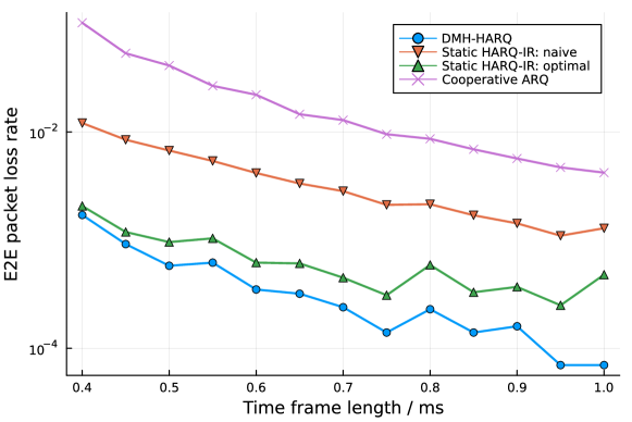
Figure 2: Sensitivity test regarding the time frame length

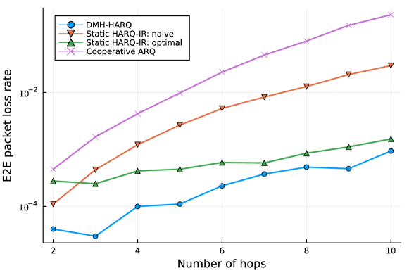
Figure 3: Sensitivity test regarding the number of hops

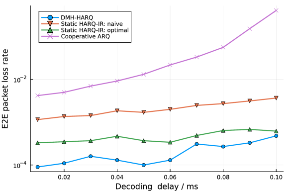
Figure 4: Sensitivity test regarding the decoding/feedback delay

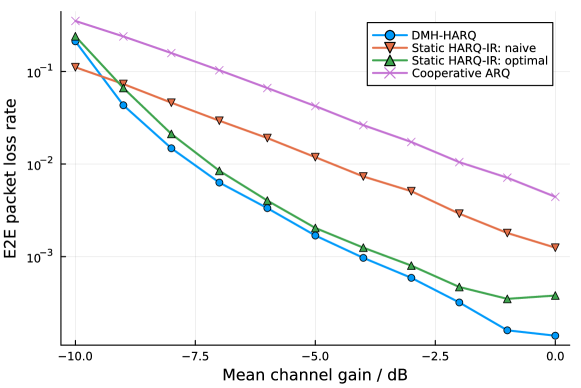
Figure 5: Sensitivity test regarding the path loss

VI Further Discussions

VI-A IR Gain

We have proven that even when applied without any combining technique, DMH-HARQ is able to outperform the optimal static HARQ-IR. A natural idea, of course, is to further enhance the performance of DMH-HARQ with soft combining, especially with an ideal IR, where the PER formula (8) must be replaced by

$$\varepsilon_{s}=Q\left(\sqrt{\frac{n_{s}+\frac{\tau_{s}}{T_{\mathrm{b}}}}{V_{I+1-i_{s}}}}\left(\mathcal{C}_{I+1-i_{s}}-\frac{d}{n_{s}+\frac{\tau_{s}}{T_{\mathrm{b}}}}\right)\ln 2\right).$$ (14)

Though IR is guaranteed to reduce the achievable E2E packet loss rate of DMH-HARQ, it costs more computational effort. The inclusion of $\tau_{s}$ into $\varepsilon_{s}$ rejects Lemma 1. To keep it an MDP so that the integer DP based framework of Algorithm 1 still applies, $\tau_{s}$ must play its role as part of the system state when solving the decision policy, i.e. $n_{s}$. The dictionaries $\mathcal{D}_{\mathrm{local}}$ and $\mathcal{D}_{\mathrm{succ}}$ in Algorithm 1 shall map $[t_{s},i_{s},\tau_{s}]$ instead of $[t_{s},i_{s}]$ to $[\xi_{\mathrm{opt}},n_{\mathrm{opt}}]$. This will significantly increase the effective size of the state space, raising the time complexity of solving $n_{s}$ at each node from $\mathcal{O}(n_{\mathrm{MAX}}^{I})$ to $\mathcal{O}(n_{\mathrm{MAX}}^{2I})$.

VI-B Multi-Access Design

In this paper we have been focusing on a single multi-hop data link. In practical deployment, a multi-access solution will be mandatory to allow efficient networking - especially in the fronthaul and midhaul domains, where the network exhibits a star topology that each DU is associated with multiple RUs and each CU with multiple DUs. While orthogonal frequency-division multiple access (OFDMA) is widely used in modern radio systems and has been dominating most wireless standards, it may not be the optimal match for our DMH-HARQ protocol, due to the challenge in interference management caused by the dynamic traffic pattern that are hard to predict. Similar issue has already been discussed for the original CLARQ problem [10], revealing that time-division multiple access (TDMA) will be a better solution than OFDMA in this context. This will limit the application of the dynamic HARQ approaches such like CLARQ or DMH-HARQ for the air interface between users and base stations, which are generally standardized in modern cellular systems to use OFDMA for better scalability and flexibility. It is also for this reason that we exclude the air interface from the scope of this study.

However, in wireless transport networks which is under our focus in this study, TDMA can still be a good and feasible option, because: i) unlike the air interface of Radio Access Network (RAN), the physical layer design of transport network is not universally standardized but upon the design of vendor, allowing to use TDMA; ii) compared to the number of user equipments (UEs) in RAN, the number of transport network nodes are limited, leading to low demand for scalability; iii) the transport network nodes are generally installed at fixed position, leading to easy synchronization and low demand for flexibility.

Moreover, the TDMA design in DMH-HARQ can be potentially combined with the target wake time (TWT) mechanism, which is utilized by the IEEE 802.11ax standard, to further raise the time efficiency of DMH-HARQ: after successfully forwarding a message, the relaying node can send a triggering token to the next transmitting node, so that it is immediately waken from sleep and start its the DMH-HARQ process, instead of waiting till the last transmitting node completing its multi-hop relay. In such way, multiple data links can be parallelized in a pipeline fashion over the multiple hops, so that the E2E delay is reduced.

VII Related Work

The problem of multi-hop relay has been attracting great interest in the wireless field since long, for it has a rich potential to offer extended cell coverage and improved channel capacity [1], particularly in the O-RAN architecture [13, 14]. Generally, there are two families of relay technologies, namely DF and amplify-and-forward (AF). Albeit the disadvantage of higher implementation complexity, DF comprehensively outperforms AF in latency-reliability performance [15], and is therefore preferred by many researchers. Literature has investigated multi-hop DF from various perspectives, including modulation scheme [16], selective relaying route [17], and relay station placement [18], and ARQ strategy [19].

Over the past few years, the emerging wireless use scenario of URLLCin O-RAN is challenging off-the-shelf multi-hop relay. The extreme requirement of low E2E latency in O-RAN URLLC is leading to even more stringent time constraint over each individual hop [20, 21], which is barely achievable with conventional technologies. To meet such a stringent latency requirement, URLLC transmissions are likely carried out with short packet, i.e., the codewords cannot considered as infinite long. With such so-called FBL codes, many theories and propositions in classical information theory fail to apply since the Shannon limit is no more asymptotically achievable. To accurately characterize the relationship between achievable data rate and reliability in the FBL regime, Polyanskiy et al. derived in [9] a closed-form expression for the single-hop transmission in AWGN channels. Later on, this FBL characterization was generalized, extended into Gilbert-Elliot channels [22] and quasi-static flat-fading channels [23]. Recently, the FBL model in random access channel has also been analyzed [24]. On the basis of those results, the performance FBL communication systems has been investigated in context of various wireless networking technologies, such as multi-input multi-output (MIMO) [25], OFDMA [26], non-orthogonal multiple access (NOMA) [27] and multi-access edge computing (MEC) [28].

Specifically for FBL relay networks, the system performance are generally investigated in a deterministic manner in the most existing works [3, 29, 30, 31, 32]. In particular, the authors of [3] studied the performance bound of two-hop FBL relay system with perfect CSI, which was later extended to the scenarios with only partial CSI available [29]. Moreover, the authors of [30] investigated a potential use case where unmanned aerial vehicle (UAV) behaves as the relay between source and destination to improve the system performance. Energy harvesting was introduced in [31] where the relay solely relies on the harvested energy to forward the information. The authors of [32] studied the impact of imperfect successive interference cancellation (SIC) in NOMA schemes on relay system that causes by the FBL transmission error.

Another interesting FBL use case is the closed-loop communication, which is not only common in MECscenarios but also strongly related to FBL relay networks, because it behaves in a similar way as a two-hop relay chain does. The authors of [10] proposed for this use case the so-called CLARQ algorithm, which dynamically re-allocates blocklengths between uplink retransmission and downlink reception, so as to minimize the closed-loop error rate. Moreover, in [33] they analyzed the optimal one-shot transmission scheme, which is a special case of CLARQ, under both constraints of latency and energy consumption.

VIII Conclusion and Outlooks

In this paper, we have studied the problem of dynamic HARQ in multi-hop wireless transport network with a special focus on reliability and openness. Focusing on the FBL regime, we proposed a DMH-HARQ scheme and an associated DP algorithm to optimize it. The proposed methods are proven by numerical simulations as effective and outperforming conventional baselines, even when without any code combining.

As for the next step, we are looking forward to applying IR to DMH-HARQ, and extending our analyses and optimization methods in this paper thereto. Deeper study to the multiple access design for DMH-HARQ and its integration with TWT mechanism is also an interesting topic for future study.

Appendix A Proof of Lemma 2

Proof.

For the last hop ($i_{s}=1$), consider an arbitrary DMH-HARQ scheme with maximal $K$ transmission attempts, where the blocklength of $k^{\mathrm{th}}$ (re-)transmission is $m_{k}$ for all $k\in\{1,2,\dots K\}$. Obviously, since $i_{s}=1$, the utility equals the overall chance of successful transmission. Using Type I HARQ without combining, that is

$$\begin{split}\xi=&1-\epsilon_{I}(m_{1})+\epsilon_{I}(m_{1})\left[1-\epsilon_{I}(m_{2})\right]\\ &+\epsilon_{I}(m_{1})\epsilon_{I}(m_{2})\left[1-\epsilon_{I}(m_{3})\right]+\dots\\ &+\epsilon_{I}(m_{1})\dots\epsilon_{I}(m_{K-1})\left[1-\epsilon_{I}(m_{K})\right]\\ =&1-\prod\limits_{k=1}^{K}\epsilon_{I}(m_{k})\end{split}$$ (15)

Meanwhile, according to [4], if it is Type-II HARQ with IR applied, the overall chance of successful transmission is equivalent to that of an one shot transmission:

$$\xi_{\mathrm{os}}=1-\epsilon_{I}\left(\sum\limits_{k=1}^{K}m_{k}\right).$$ (16)

Obviously, under the same blocklength allocation and channel conditions, Type II HARQ-IR always outperforms Type I HARQ without combining in error rate, i.e., $\prod\limits_{k=1}^{K}\epsilon_{I}(m_{k})\geqslant\epsilon_{I}\left(\sum\limits_{k=1}^{K}m_{k}\right)$, which takes the equality only when $K=1$. Furthermore, given the fixed remaining time $t_{s}$, we always have the constraint $\sum\limits_{k=1}^{K}\left(m_{k}T_{\mathrm{b}}+T_{\mathrm{l}}\right)\leqslant t_{s}$, which means

$$\sum\limits_{k=1}^{K}m_{k}\leqslant\frac{t_{s}-KT_{\mathrm{l}}}{T_{\mathrm{b}}}\leqslant\frac{t_{s}-T_{\mathrm{l}}}{T_{\mathrm{b}}},$$ (17)

where the first equality is taken only when $t_{s}$ is sufficiently exploited, and the second taken only when $K=1$. Additionally, i always holds that $\partial\epsilon_{I}(m)/\partial m<0$ for all $m\in\mathbb{R}^{+}$. Thus, we have

$$\prod\limits_{k=1}^{K}\epsilon_{I}(m)\geqslant\epsilon_{I}\left(\frac{t_{s}-T_{\mathrm{l}}}{T_{\mathrm{b}}}\right),$$ (18)

where the equality is only taken when $K=1$ and $m_{1}=\frac{t_{s}-T_{\mathrm{l}}}{T_{\mathrm{b}}}$, and the Lemma is therewith proven.

∎

Appendix B Proof of Theorem 1

Proof.

For the first step, we prove the monotone of $\xi_{\mathrm{max}}(s)$ regarding $t_{s}$ as follows. Given any feasible system status $s_{0}=(t_{s_{0}},i_{s_{0}},k_{s_{0}},\tau_{s_{0}})$, let $n_{\mathrm{opt}}$ be an optimal blocklength allocation policy that generates the DMH-HARQ schedule $\mathfrak{T}_{s_{0}}^{\mathrm{opt}}$ with maximized utility $\xi_{\mathrm{max}}(s_{0})$. According to Lemma 2, there must be $n_{\mathrm{opt}}(s)=\frac{t_{s}}{T_{\mathrm{b}}}-T_{\mathrm{l}}$ for all $s$ that $i_{s}=1$.

Given an arbitrary $\Delta t>0$, let $s^{<\Delta t>}$ denote $(t_{s}+\Delta t,i_{s},k_{s},\tau_{s})$, we can always construct a sub-optimal $n_{\mathrm{sub}}$ that

$$n_{\mathrm{sub}}(s)=\begin{cases}n_{\mathrm{opt}}(s^{<-\Delta t>})+\frac{\Delta t}{T_{\mathrm{b}}}&i_{s}=1,\\ n_{\mathrm{opt}}(s^{<-\Delta t>})&\mathrm{otherwise}.\end{cases}$$ (19)

Now apply $n_{\mathrm{sub}}$ on the initial state $s_{1}=s_{0}^{\Delta t}$ to generate another DMH-HARQ schedule $\mathfrak{T}^{\mathrm{sub}}_{s_{1}}$, it is straightforward to derive that $\mathfrak{T}^{\mathrm{opt}}_{s_{0}}$ and $\mathfrak{T}^{\mathrm{opt}}_{s_{1}}$ have the identical structure, except that for each non-empty node $s$ in $\mathfrak{T}^{\mathrm{opt}}_{s_{0}}$, the corresponding node of $\mathfrak{T}^{\mathrm{opt}}_{s_{1}}$ is

$$s^{\prime}=\begin{cases}s&i_{s^{\prime}}=0,\\ s^{<\Delta t>}&\text{otherwise}.\end{cases}$$ (20)

And error rates of each transmission attempt regarding the two schedules, denoted as $\varepsilon_{s}$ and $\varepsilon^{\prime}_{s^{\prime}}$, respectively, must fulfill

$$\varepsilon^{\prime}_{s^{\prime}}\begin{cases}<\varepsilon_{s}&i_{s^{\prime}}=1,\\ =\varepsilon_{s}&\text{otherwise}.\end{cases}$$ (21)

Recalling Eq. (12), it always hold $\xi(\mathfrak{T}^{\mathrm{sub}}_{s_{1}})>\xi_{\mathrm{max}}(s_{0})$. Meanwhile, there is always some $n^{\prime}_{\mathrm{opt}}$ that generates an optimal schedule $\mathfrak{T}^{\mathrm{opt}}_{s_{1}}$ with maximal $\xi_{\mathrm{max}}(s_{1})\geqslant\xi(\mathfrak{T}^{\mathrm{sub}}_{s_{1}})$. Thus:

$$\xi_{\mathrm{max}}(s_{1})=\xi_{\mathrm{max}}(s_{0}^{<\Delta t>})>\xi_{\mathrm{max}}(s_{0})\quad\forall s_{0},\forall\Delta t>0,$$ (22)

i.e. $\xi_{\mathrm{max}}(s)$ is strictly monotone increasing regarding $t_{s}$.

Next, we come to prove the continuity of this function. According to Eq. (8), $\varepsilon_{s}$ is continuous function of $t_{s}$, so $\xi_{\mathrm{max}}(s)$ can be guaranteed $t_{s}$-continuous, if both $\xi_{\mathrm{max}}(s_{\mathrm{l}}(\mathfrak{T}_{s}))$ and $\xi_{\mathrm{max}}(s_{\mathrm{r}}(\mathfrak{T}_{s}))$ are continuous functions of $t_{s}$. This sufficient condition can be derived via mathematical induction as follows.

Starting with the two termination cases of $t_{s}<T_{\mathrm{min}}^{(i_{s})}$ and $i_{s}=0$, respectively, according to Eqs. (1) and (2) we have $S(L(\mathfrak{T}_{s}))=S(R(\mathfrak{T}_{s}))=\emptyset$. Recalling (5), for the termination cases we have $\xi_{\mathrm{max}}(s)=\xi(\mathfrak{T}_{s})\equiv 0$, which are both $t_{s}$-continuous. Therefore, the utility $\xi_{\mathrm{max}}(s)$ itself is also $t_{s}$-continuous.

Then consider the last hop where $i_{s}=1$, according to Lemma 2 we know that $\xi_{\mathrm{max}}(s)$ is achieved when $n_{s}=\frac{t_{s}-T_{\mathrm{l}}}{T_{\mathrm{b}}}$, leading to a left branch where $t_{s_{\mathrm{l}}(\mathfrak{T}_{s})}=0<T_{\mathrm{min}}^{(1)}$ and a right branch where $i_{s_{\mathrm{r}}(\mathfrak{T}_{s})}=0$, both are termination cases. Thus, as proven above we have both $\xi_{\mathrm{max}}(s_{\mathrm{l}}(\mathfrak{T}_{s}))$ and $\xi_{\mathrm{max}}(s_{\mathrm{r}}(\mathfrak{T}_{s}))$ are $t_{s}$-continuous, and therefore $\xi_{\mathrm{max}}(s)$ the same as well.

For other hops other than the last one, i.e. $i_{s}\in\{2,3,\dots I\}$, according to the DMH-HARQ principle (1) and (2), it is obvious that there are only three possible combinations of its left and right branches:

1. $s_{\mathrm{l}}(\mathfrak{T}(s))=\emptyset,i_{s_{\mathrm{r}}(\mathfrak{T}(s))}=\emptyset$;

2. $s_{\mathrm{l}}(\mathfrak{T}(s))=\emptyset,i_{s_{\mathrm{r}}(\mathfrak{T}(s))}=i_{s}-1$;

3. $i_{s_{\mathrm{l}}(\mathfrak{T}(s))}=i_{s},i_{s_{\mathrm{r}}(\mathfrak{T}(s))}=i_{s}-1$.

For case 1), $\xi_{\mathrm{max}}(s)\equiv 0$, which is $t_{s}$-continuous. For case 2), $\xi_{\mathrm{max}}(s_{\mathrm{l}}(\mathfrak{T}_{s}))$ is $t_{s}$-continuous as proven above, so that $\xi_{\mathrm{max}}(s)$ can be guaranteed $t_{s}$-continuous if only $\xi_{\mathrm{max}}(s_{\mathrm{r}}(\mathfrak{T}_{s}))$ is $t_{s}$-continuous. For case 3), we recall Lemma 1 that $n_{\mathrm{opt}}(s)$ depends only on $t_{s}$ and $i_{s}$, so that $\xi_{\mathrm{max}}(\mathfrak{T}(s))$ and $\xi_{\mathrm{max}}(L(\mathfrak{T}(s)))$ are different samples for the same function of $t_{s}$. Since the iterative generation of the left branch in decision tree is determined to terminate with an empty set, i.e. case 1) or 2), we can conclude that for a $\mathfrak{T}s$ in case 3), both $\xi_{\mathrm{max}}(s)$ and $\xi_{\mathrm{max}}(s_{\mathrm{l}}(\mathfrak{T}(s)))$ are guaranteed $t_{s}$-continuous if $\xi_{\mathrm{max}}(s_{\mathrm{r}}(\mathfrak{T}_{s}))$ is $t_{s}$-continuous. Since the iterative generation of the right branch in decision tree always ends up with one of the two termination cases, which are both $t_{s}$-continuous, we can conclude from the analyses above that $\xi_{\mathrm{max}}(s)$ is also $t_{s}$-continuous for all $s$ where $i_{s}>1$.

Thus, the continuity is proven for all $i\in\mathcal{S}$. With both the monotone and the continuity derived, the theorem is proven. ∎

Bin Han (Senior Member, IEEE) received his B.E. degree in 2009 from Shanghai Jiao Tong University, M.Sc. in 2012 from the Technical University of Darmstadt, and a Ph.D. degree in 2016 from Karlsruhe Institute of Technology. Since July 2016 he has been with the Division of Wireless Communications and Radio Positioning, Rheinland-Pfälzische Technische Universität Kaiserslautern-Landau (formerly: Technische Universität Kaiserslautern) as a Postdoctoral Researcher and Senior Lecturer. His research interests are in the broad areas of wireless communications, networking, and signal processing. He is the author of one book, five book chapters, and over 50 research papers. He has participated in multiple EU FP7, Horizon 2020, and Horizon Europe research projects. Dr. Han is Editorial Board Member for Network and Guest Editor for Electronics. He has served in organizing committee and/or TPC for IEEE GLOBECOM, IEEE ICC, EuCNC, European Wireless, and ITC. He is a Voting Member of the IEEE Standards Association Working Groups P2303 and P3106.

Muxia Sun (Member, IEEE) received in 2010 his B.Sc. degree from South China University of Technology (SCUT), M.Sc. in 2012 & 2013 from Université de Nantes and SCUT, respectively, and the Ph.D. degree in 2019 from Université Paris-Saclay. Since 2020 he has been with Tsinghua University as Postdoctoral Researcher in the Department of Industrial Engineering. His current research interests include reliability assessment and optimization of industrial & communication systems, robust optimization, and approximation algorithm design.

Yao Zhu (Member, IEEE) received the B.S. degree in electrical engineering from the University of Bremen, Bremen, Germany, in 2015,  his master’s degree and  his P.h.D degree in electrical engineering, information technology and computer engineering from RWTH Aachen University, Aachen, Germany, in 2018 and 2022, respectively. He is currently a postdoctoral researcher with the Chair of Information Theory and Data Analytics. His research interests include ultra-reliable and low-latency communications, integrated sensing and communication, as well as physical layer security.

Vincenzo Sciancalepore (Senior Member, IEEE) received his M.Sc. degree in Telecommunications Engineering and Telematics Engineering in 2011 and 2012, respectively, whereas in 2015, he received a double Ph.D. degree. Currently, he is a senior 5G researcher at NEC Laboratories Europe GmbH in Heidelberg, focusing his activity on Smart Surfaces and Reconfigurable Intelligent Surfaces (RIS). He is currently involved in the IEEE Emerging Technologies Committee leading the initiatives on RIS. He was also the recipient of the national award for the best Ph.D. thesis in the area of communication technologies (Wireless and Networking) issued by GTTI in 2015. He is an Editor of IEEE Transactions on Wireless Communications.

Mohammad Asif Habibi received his B.Sc. degree in Telecommunications Engineering from Kabul University, Afghanistan, in 2011. He obtained his M.Sc. degree in Systems Engineering and Informatics from the Czech University of Life Sciences, Czech Republic, in 2016. Since January 2017, he has been working as a research fellow and Ph.D. candidate at the Division of Wireless Communications and Radio Positioning, Rheinland-Pfälzische Technische Universität Kaiserslautern-Landau (previously known as Technische Universität Kaiserslautern), Germany. From 2011 to 2014, he worked as a radio access network engineer for HUAWEI. His main research interests include network slicing, network function virtualization, resource allocation, machine learning, and radio access network architecture.

Yulin Hu (Senior Member, IEEE) received his M.Sc.E.E. degree from USTC, China, in 2011. In Dec. 2015 he received his Ph.D.E.E. degree (Hons.) from RWTH Aachen University where he was a postdoctoral Research Fellow since Jan. to Dec. in 2016. He was a senior researcher and team leader in ISEK research Area at RWTH Aachen University. From May to July in 2017, he was a visiting scholar in Syracuse University, USA. He is currently a professor with School of Electronic Information, Wuhan University, and an adjunct professor with ISEK research Area, RWTH Aachen University. His research interests are in information theory, optimal design of wireless communication systems. He has been invited to contribute submissions to multiple conferences. He was a recipient of the IFIP/IEEE Wireless Days Student Travel Awards in 2012. He received the Best Paper Awards at IEEE ISWCS 2017 and IEEE PIMRC 2017, respectively. He served as a TPC member for many conferences. He was the lead editor of the URLLC-LoPIoT spacial issue in Physical Communication, and the organizer and chair of two special sessions in IEEE ISWCS 2018 and ISWCS 2020. He is currently serving as an editor for Physical Communication (Elsevier), EURASIP Journal on Wireless Communications and Networking, and Frontiers in Communications and Networks.

Anke Schmeink (Senior member, IEEE) received the Diploma degree in mathematics with a minor in medicine and the Ph.D. degree in electrical engineering and information technology from RWTH Aachen University, Germany, in 2002 and 2006, respectively. She worked as a research scientist for Philips Research before joining RWTH Aachen University in 2008 where she is a professor since 2012. She spent several research visits with the University of Melbourne, and with the University of York. Anke Schmeink is a member of the Young Academy at the North Rhine-Westphalia Academy of Science. Her research interests are in information theory, machine learning, data analytics and optimization with focus on wireless communications and medical applications.

Yan-Fu Li (Senior Member, IEEE) was a Faculty Member with the Laboratory of Industrial Engineering, CentraleSupélec, University of Paris-Saclay, Gif-sur-Yvette, France, from 2011 to 2016. He is currently a Professor with the Industrial Engineering Department, Tsinghua University, Beijing, China. He has led/participated in several projects supported by the European Union (EU), France, and Chinese Governmental funding agencies and various industrial partners. He has coauthored or coauthored more than 100 publications on international journals, conference proceedings, and books. His current research interests include reliability, availability, maintainability, and safety (RAMS) assessment and optimization with the applications onto various industrial systems. Dr. Li is an Associate Editor of IEEE Transactions on Reliability.

Hans D. Schotten (Member, IEEE) received the Ph.D. degree from the RWTH Aachen University, Germany, in 1997. From 1999 to 2003, he worked for Ericsson. From 2003 to 2007, he worked for Qualcomm. He became manager of a R&D group, Research Coordinator for Qualcomm Europe, and Director for Technical Standards. In 2007, he accepted the offer to become a Full Professor at Technische Universität Kaiserslautern. In 2012, he - in addition - became the Scientific Director of the German Research Center for Artificial Intelligence (DFKI) and Head of Department for Intelligent Networks. Professor Schotten served as Dean of Department of Electrical and Computing Engineering at Technische Universität Kaiserslautern from 2013 until 2017. Since 2018, he is the Chair of the German Society for Information Technology and a member of the Supervisory Board of the VDE. He has authored more than 200 papers and participated in over 30 European and national collaborative research projects.

References

- [1] N. Athanasopoulos, P. Tsiakas, K. Voudouris, I. Georgas, and G. Agapiou, “Multi-hop relay in next generation wireless broadband access networks: An overview,” in International Conference on Mobile Lightweight Wireless Systems. Springer, 2010, pp. 543–554.
- [2] S. Karmakar and M. K. Varanasi, “The diversity-multiplexing tradeoff of the dynamic decode-and-forward protocol on a MIMO half-duplex relay channel,” IEEE Transactions on Information Theory, vol. 57, no. 10, pp. 6569–6590, 2011.
- [3] Y. Hu, J. Gross, and A. Schmeink, “On the capacity of relaying with finite blocklength,” IEEE Transactions on Vehicular Technology, vol. 65, no. 3, pp. 1790–1794, 2016.
- [4] B. Makki, T. Svensson, and M. Zorzi, “Finite block-length analysis of the incremental redundancy HARQ,” IEEE Wireless Communications Letters, vol. 3, no. 5, pp. 529–532, 2014.
- [5] Samsung, “Virtualized radio access network: architecture, key technologies and benefits.” Technical Report, 2019.
- [6] A. Garcia-Saavedra and X. Costa-Pérez, “O-ran: Disrupting the virtualized ran ecosystem,” IEEE Communications Standards Magazine, vol. 5, no. 4, pp. 96–103, 2021.
- [7] G. Garcia-Aviles, A. Garcia-Saavedra, M. Gramaglia, X. Costa-Perez, P. Serrano, and A. Banchs, “Nuberu: Reliable ran virtualization in shared platforms,” in Proceedings of the 27th Annual International Conference on Mobile Computing and Networking, ser. MobiCom ’21. New York, NY, USA: Association for Computing Machinery, 2021, p. 749–761.
- [8] J. Gomes, J. A. L. Silva, and M. E. V. Segatto, “Reducing the 5G fronthaul traffic with O-RAN,” in 2019 SBMO/IEEE MTT-S International Microwave and Optoelectronics Conference (IMOC), 2019, pp. 1–3.
- [9] Y. Polyanskiy, H. V. Poor, and S. Verdú, “Channel coding rate in the finite blocklength regime,” IEEE Transactions on Information Theory, vol. 56, no. 5, pp. 2307–2359, 2010.
- [10] B. Han, Y. Zhu, M. Sun, V. Sciancalepore, Y. Hu, and H. D. Schotten, “CLARQ: A dynamic ARQ solution for ultra-high closed-loop reliability,” IEEE Transactions on Wireless Communications, vol. 21, no. 1, pp. 280–294, 2022.
- [11] J. Goel and H. Jagadeesh, “Listen to others’ failures: Cooperative ARQ schemes for low-latency communication over multi-hop networks,” IEEE Transactions on Wireless Communications, vol. 20, no. 9, pp. 6049–6063, 2021.
- [12] R. Bellman, “Some problems in the theory of dynamic programming,” Econometrica: Journal of the Econometric Society, pp. 37–48, 1954.
- [13] O-RAN Alliance, “Working Group 7; Outdoor Micro Cell Hardware Architecture and Requirements (FR1) Specification; V01.00,” Alfter, Germany, Jun. 2021.
- [14] M. Mohsin, J. M. Batalla, E. Pallis, G. Mastorakis, E. K. Markakis, and C. X. Mavromoustakis, “On analyzing beamforming implementation in O-RAN 5G,” Electronics, vol. 10, no. 17, 2021.
- [15] A. Chaaban and A. Sezgin, “Multi-hop relaying: An end-to-end delay analysis,” IEEE Transactions on Wireless Communications, vol. 15, no. 4, pp. 2552–2561, 2016.
- [16] K. Dhaka, R. K. Mallik, and R. Schober, “Performance analysis of decode-and-forward multi-hop communication: A difference equation approach,” IEEE Transactions on Communications, vol. 60, no. 2, pp. 339–345, 2012.
- [17] G. Farhadi and N. C. Beaulieu, “Fixed relaying versus selective relaying in multi-hop diversity transmission systems,” IEEE Transactions on Communications, vol. 58, no. 3, pp. 956–965, 2010.
- [18] J. Ibrahim, A. Rehman, M. S. B. Ilyas, M. Shehzad, and M. Ashraf, “Optimization and traffic management in IEEE 802.16 multi-hop relay stations using genetic and priority algorithms,” International Journal of Computer Science and Information Security, vol. 14, no. 7, p. 599, 2016.
- [19] S. Maagh, M. Y. Sharif, and A. Almaini, “On the dynamic decode-and-forward relay listen-transmit decision rule in intersymbol interference channels,” in Proceedings of the 9th WSEAS international conference on Data networks, communications, computers, 2010, pp. 26–29.
- [20] M. A. Habibi, F. Z. Yousaf, and H. D. Schotten, “Mapping the VNFs and VLs of a RAN slice onto intelligent PoPs in beyond 5G mobile networks,” IEEE Open Journal of the Communications Society, vol. 3, pp. 670–704, 2022.
- [21] C. C. Zhang, K. K. Nguyen, and M. Cheriet, “Joint routing and packet scheduling for URLLC and eMBB traffic in 5G O-RAN,” in ICC 2022 - IEEE International Conference on Communications, 2022, pp. 1900–1905.
- [22] Y. Polyanskiy, H. V. Poor, and S. Verdú, “Dispersion of the Gilbert-Elliott channel,” in 2009 IEEE International Symposium on Information Theory, 2009, pp. 2209–2213.
- [23] W. Yang, G. Durisi, T. Koch, and Y. Polyanskiy, “Quasi-static multiple-antenna fading channels at finite blocklength,” IEEE Transactions on Information Theory, vol. 60, no. 7, pp. 4232–4265, 2014.
- [24] M. Effros, V. Kostina, and R. C. Yavas, “Random access channel coding in the finite blocklength regime,” in 2018 IEEE International Symposium on Information Theory (ISIT), 2018, pp. 1261–1265.
- [25] X. Zhang, J. Wang, and H. V. Poor, “Statistical delay and error-rate bounded QoS provisioning for mURLLC over 6g CF M-MIMO mobile networks in the finite blocklength regime,” IEEE Journal on Selected Areas in Communications, vol. 39, no. 3, pp. 652–667, 2021.
- [26] B. Han, Y. Zhu, Z. Jiang, M. Sun, and H. D. Schotten, “Fairness for freshness: Optimal age of information based OFDMA scheduling with minimal knowledge,” IEEE Transactions on Wireless Communications, vol. 20, no. 12, pp. 7903–7919, 2021.
- [27] X. Sun, S. Yan, N. Yang, Z. Ding, C. Shen, and Z. Zhong, “Short-packet downlink transmission with non-orthogonal multiple access,” IEEE Trans. Wireless Commun., vol. 17, no. 7, pp. 4550–4564, 2018.
- [28] Y. Zhu, Y. Hu, A. Schmeink, and J. Gross, “Energy minimization of mobile edge computing networks with HARQ in the finite blocklength regime,” IEEE Transactions on Wireless Communications, pp. 1–1, 2022.
- [29] Y. Hu, A. Schmeink, and J. Gross, “Optimal scheduling of reliability-constrained relaying system under outdated CSI in the finite blocklength regime,” IEEE Transactions on Vehicular Technology, vol. 67, no. 7, pp. 6146–6155, 2018.
- [30] C. Pan, H. Ren, Y. Deng, M. Elkashlan, and A. Nallanathan, “Joint blocklength and location optimization for URLLC-enabled UAV relay systems,” IEEE Communications Letters, vol. 23, no. 3, pp. 498–501, 2019.
- [31] Y. Hu, Y. Zhu, M. C. Gursoy, and A. Schmeink, “SWIPT-enabled relaying in IoT networks operating with finite blocklength codes,” IEEE Journal on Selected Areas in Communications, vol. 37, no. 1, pp. 74–88, 2019.
- [32] A. Agarwal, A. K. Jagannatham, and L. Hanzo, “Finite blocklength non-orthogonal cooperative communication relying on SWIPT-enabled energy harvesting relays,” IEEE Transactions on Communications, vol. 68, no. 6, pp. 3326–3341, 2020.
- [33] B. Han, Y. Zhu, A. Schmeink, and H. D. Schotten, “Time-energy-constrained closed-loop FBL communication for dependable MEC,” in 2021 IEEE Conference on Standards for Communications and Networking (CSCN). IEEE, 2021, pp. 180–185.