Manifold Learning for Dimensionality Reduction: Quantum Isomap algorithm

Abstract

Isomap algorithm is a representative manifold learning algorithm. The algorithm simplifies the data analysis process and is widely used in neuroimaging, spectral analysis and other fields. However, the classic Isomap algorithm becomes unwieldy when dealing with large data sets. Our object is to accelerate the classical algorithm with quantum computing, and propose the quantum Isomap algorithm. The algorithm consists of two sub-algorithms. The first one is the quantum Floyd algorithm, which calculates the shortest distance for any two nodes. The other is quantum Isomap algorithm based on quantum Floyd algorithm, which finds a low-dimensional representation for the original high-dimensional data. Finally, we analyze that the quantum Floyd algorithm achieves exponential speedup without sampling. In addition, the time complexity of quantum Isomap algorithm is $O(dNpolylogN)$. Both algorithms reduce the time complexity of classical algorithms.

I introduction

With the continuous popularization of "digitalization", a large amount of information produced in real life is digitized. In the digital age, it has become essential to store content such as text, webpages and images with fewer resources. The challenge of using high-dimensional data for machine learning tasks, moreover, are not conducive to training. Among problems are inescapable for all machine learning methods, which is called the "curse of dimensionality" [1]. For these problems, there are two common solutions. The first one is to increase the number of samples and, thus, improve the density of training set. However, this is infeasible since the complexity is exponential. Another approach is widely accepted, which is called dimensionality reduction [2, 3, 4]. By filtering out non-essential features of high-dimensional samples, the proposed method can obtain a low-dimensional representation of the original high-dimensional data. In general, dimensionality reduction methods can be categorized as linear or nonlinear methods. The basic idea of the former is to find low-dimensional projections and extract essential information from the data. The latter assumes the original high-dimensional data distributed on the low-dimensional manifold, and reconstructs the original data on the low-dimensional manifold. In addition, these methods are widely used in fields such as pattern recognition, image processing and text analysis.
Undoubtedly, dimensionality reduction algorithms address data storage and improve the learning efficiency of machine learning models. However, this algorithm yields a high time complexity. Given a data matrix of $N\times D$, where $N$ and $D$ represent the number of samples and the dimension of samples, respectively, the time complexity is $O(N^{3})$. On the other hand, quantum computation is one of the important areas of quantum information technology. Since the propositions of Shor algorithm [5] and Grover algorithm [6], the quantum computing [7, 8] have attracted much attention. Recently, there has been a lot of research on combining machine learning tasks with quantum computing. This further stimulates us to investigate to reduce the time complexity of dimension reduction algorithms with quantum computing.
So far, researchers have proposed some quantum versions of dimensionality reduction algorithms. In 2014, Professor Loyd’s group [9] came up with the first dimensional reduction algorithm, quantum principal component analysis, which provided a reference for many subsequent quantum algorithms. The algorithm aims to maximize the variance of the projected samples using the projection matrix, and eventually achieve dimensionality reduction. Formally, quantum principal component analysis algorithm achieves the exponential acceleration compared with the classical algorithm counterpart. In 2016, Cong et al. [10] proposed a quantum linear discriminant algorithm. The algorithm calculates the ratio of between-class scatter degree to within-class scatter degree, and seeks the optimal projection direction of the data. The overall time complexity of the algorithm is polylogarithmic in both the number of samples and the dimension. Both quantum algorithms speed up the processing of linear dimensionality reduction tasks. However, linear dimensionality reduction algorithms are powerless when the original data is distributed on the manifold. Then, He et al. [11] proposed a quantum version of local linear embeding algorithm in 2020. The algorithm assumes the data exists linear relationship between the data and the locally adjacent points, which remains unchanged the relation after dimensionality reduction. Soon after, Li [12] proposed a quantum nonlinear dimensionality reduction algorithm based on arbitrary kernel functions. The idea of the algorithm is to approximate arbitrary kernels using the idea of Taylor series. It should be noted that the algorithm performance will vary greatly when selecting different kernel functions. In 2021, Sornsaeng [13] proposed a quantum diffusion mapping algorithm inspired by random walks. In fact, the algorithm converts the sample similarity matrix to the analysis of the transition matrix, and the higher similarity corresponds to the higher transition probability.
In contrast to the above facts, performing these nonlinear dimensionality reduction algorithms on manifold data, the effect between data pairs that are far apart cannot be guaranteed. In this way, we propose a quantum Isomap algorithm. Let the algorithm perform on the original dataset, and the relative relationships between all the new data will unchanged. One difficulty of our algorithm is calculating the geodesic distance. To obtain the manifold distance between all data pairs, we propose a quantum Floyd algorithm. It should be noted that the quantum Floyd algorithm must effectively load the adjacency matrix, for example, using the quantum random access memory. As a part of the Isomap algorithm, the quantum Floyd algorithm enables us to efficiently complete the algorithm. In addition, we use the quantum singular value estimation algorithm to estimate the eigen-solution of the inner product matrix. Both algorithms provide a significant acceleration effect.
The remainder of the paper is organized as follows: Section II introduces the classical Isomap algorithm and the quantum singular value estimation. Section III gives the quantum Isomap algorithm and its sub-algorithm. Section IV analyzes the time complexity of the proposed algorithm. Finally, we give relevant conclusions in Sec.V.

II preliminaries

In this section, we review the basic idea and the main procedure of the classical Isomap algorithm. Then, we introduce the quantum singular value estimate and give some necessary derivation steps.

II.1 Review of Classical Isomap algorithm

The Isomap algorithm is a nonlinear dimensionality reduction method. The algorithm takes geodesic distance as the input of MDS algorithm, and calculate the low-dimensional results of high-dimensional data. In this subsection, the classical Isomap algorithm consists of the following three steps.
In the first step, we compute the geodesic distance for all data. By using Floyd algorithm [14], we obtain the geodesic distance $d_{ij}$ between any two nodes.
The second step is to transform the geodesic distance matrix into an inner product matrix. The idea of the derivation is as follows. We assume that the data $Z\in\mathbb{R}^{N\times d}$ represents the result of dimensionality reduction. Let $K=ZZ^{T}$ the inner product matrix, where $k_{ij}=z_{i}{z_{j}}^{T}$, then

$$d_{ij}=||z_{i}||^{2}+||z_{j}||^{2}-2z_{i}{z_{j}}^{T}=k_{ii}+k_{jj}-2k_{ij}.$$ (1)

Similar to the PCA algorithm, the dataset after dimensionality reduction is assumed to be centralized. i.e., $\sum_{i}z_{i}=0$. Equivalently, the sum of the row or column of the matrix is 0, that is, $\sum_{i}{k_{ij}}=\sum_{j}{k_{ij}}=0$. We can obtain the following relationship

$$d_{i*} =\frac{1}{N}\sum_{j}{d_{ij}}=\frac{1}{N}tr(K)+k_{jj},$$ (2)

$$d_{*j} =\frac{1}{N}\sum_{i}{d_{ij}}=\frac{1}{N}tr(K)+k_{ii},$$

$$d_{**} =\frac{1}{N^{2}}\sum_{i,j}{d_{ij}}=\frac{2}{N}tr(K).$$

Here, $d_{i*}$ and $d_{*j}$ represent the row mean of the distance matrix and the column mean of the geodesic distance matrix, respectively, and $d_{**}$ is the mean of all elements of the geodesic distance matrix.
Now, we can take each entry of the inner product matrix and represent it as

$$k_{ij}=-\frac{1}{2}(d_{ij}-d_{i*}-d_{*j}+d_{**}).$$ (3)

The last step is the eigen-decomposition for the inner product matrix $K$. Since the matrix $K$ is symmetric positive semidefinite, it can be expressed as

$$K=V\Lambda V^{T},$$ (4)

where $\Lambda=diag(\lambda_{1},\lambda_{2},\cdots,\lambda_{N})$ is a diagonal matrix composed of eigenvalues, and $\lambda_{1}\geq\lambda_{2}\geq\cdots\geq\lambda_{N}$, $V$ is the eigenvector matrix arranged by the size of the eigenvalues. Equivalently, when select the $d$ largest eigenvalue, the data matrix can be represented as

$$Z=V_{*}\Lambda_{*}^{\frac{1}{2}}\in\mathbb{R}^{N\times d},$$ (5)

where $\Lambda_{*}=diag{(\lambda_{1},\lambda_{2},\cdots,\lambda_{d},0,\cdots,0)}$, $V_{*}$ is the corresponding eigenvector.

II.2 Quantum singular value estimation

Quantum singular value estimation [15, 16] is used to estimate the singular value of a matrix. Given the data structure of a matrix or the ability to prepare a matrix quantum state, we can complete the algorithm. Indeed, the algorithm is developed from a discrete-time Markov chain [17, 18]. Given a stochastic matrix $K$, we define two mappings:

$$U_{\mathcal{M}}:|0\rangle|j\rangle\to|K_{j}\rangle|j\rangle =\frac{1}{||K_{j}||}\sum_{i=1}^{M}K_{ij}|i\rangle|j\rangle,$$ (6)

$$U_{\mathcal{N}}:|i\rangle|0\rangle\to|i\rangle|K_{F}\rangle =\frac{1}{||K||_{F}}\sum_{j=1}^{M}||K_{j}|||i\rangle|j\rangle,$$

where $|K_{j}\rangle=\sum_{i=1}^{N}K_{ij}/||K_{j}|||i\rangle$, $|K_{F}\rangle=\sum_{j=1}^{N}||A_{j}||/||K||_{F}|j\rangle$. To quantize the Markov chain, we construct two matrices of the following form:

$$\mathcal{M} =\sum_{j=1}^{N}|K_{j}\rangle|j\rangle\langle j|,$$ (7)

$$\mathcal{N} =\sum_{i=1}^{N}|i\rangle|K_{F}\rangle\langle i|.$$

We prove that the product between $\mathcal{N^{\dagger}}$ and $\mathcal{M}$ satisfies

$${\mathcal{N}}^{\dagger}\mathcal{M}= {(\sum_{i=1}^{N}|i\rangle\langle i|\langle K_{F}|)}{(\sum_{j=1}^{N}|K_{j}\rangle|j\rangle\langle j|)}$$ (8)

$$= \frac{K}{||K||_{F}},$$

which corresponds to the stochastic matrix. This allows us define the following unitary transformation

$$W ={(2\mathcal{N}\mathcal{N}^{\dagger}-I_{N^{2}})}{(2\mathcal{M}\mathcal{M}^{\dagger}-I_{N^{2}})}.$$ (9)

In order to obtain the spectrum of $K$, we first isolate an invariant subspace for $W$ and look for eigenvalues and eigenvectors in this space. Let us see the effect of $W$ on $\mathcal{M}|v_{k}\rangle$

$$W\mathcal{M}|v_{k}\rangle ={(2\mathcal{N}\mathcal{N}^{\dagger}-I_{N^{2}})}{(2\mathcal{M}\mathcal{M}^{\dagger}-I_{N^{2}})}\mathcal{M}|v_{k}\rangle$$ (10)

$$=\frac{2\sigma_{k}}{||K||_{F}}\mathcal{N}|u_{k}\rangle-\mathcal{M}|v_{k}\rangle,$$

and

$$W\mathcal{N}|u_{k}\rangle=(\frac{4\sigma_{k}^{2}}{||K||_{F}^{2}}-1)\mathcal{N}|u_{k}\rangle-\frac{2\sigma_{k}}{||K||_{F}}\mathcal{M}|v_{k}\rangle,$$ (11)

where $|u_{k}\rangle$ and $|v_{k}\rangle$ are the left eigenvector and right eigenvector of $K$, respectively. From (10) and (11), we can deduce that the subspace

$$\mathcal{I}_{W}:=\{\mathcal{M}|v_{k}\rangle,\mathcal{N}|u_{k}\rangle\}$$ (12)

is invariant under $W$. Then we orthogonalize the basis using the Gram-Schmidt method [19], and get the result

$$|e_{k1}\rangle =\mathcal{M}|v_{k}\rangle,$$ (13)

$$|e_{k2}\rangle =\frac{\mathcal{N}|u_{k}\rangle-\sigma_{k}||K||_{F}^{-1}|e_{k1}\rangle}{\sqrt{1-\sigma_{k}^{2}||K||_{F}^{-2}}}.$$

By performing $W$ on $|e_{k1}\rangle$, it leads to

$$W|e_{k1}\rangle={[\frac{2\sigma_{k}^{2}}{||K||_{F}^{2}}-1]|e_{k1}\rangle}+\frac{2\sigma_{k}}{||K||_{F}}\sqrt{1-\frac{\sigma_{k}^{2}}{||K||_{F}^{2}}}|e_{k2}\rangle.$$ (14)

We consider that $\mathcal{M}|v_{k}\rangle$ and $\mathcal{N}|u_{k}\rangle$ are linearly independent [20]. Setting that $W$ rotates the basis $|e_{k1}\rangle$ in a fixed angle $2\theta$, the eigenvalue of $W$ will be $e^{2i\theta_{k}}$, and the corresponding eigenvector is $|x_{\pm}^{k}\rangle=1/\sqrt{2}(|e_{k1}\rangle\pm i|e_{k2}\rangle)$. In addition, we have the following equation relation

$$cos2\theta_{k} =\langle v_{k}|\mathcal{M}^{\dagger}W\mathcal{M}|v_{k}\rangle=2\frac{\sigma_{k}^{2}}{||K||_{F}^{2}}-1.$$ (15)

From the above expression, we obtain the relation $cos\theta_{k}=\sigma_{k}/{||K||_{F}^{2}}$, which allows us to solve the eigen-solution using quantum singular value estimation.

III Quantum Isomap algorithm

III.1 Quantum Floyd algorithm

The Floyd method is an algorithm for finding the shortest path between any two points. Since the high time complexity of the Floyd method, we propose a quantum variant of the Floyd method. When processing multi-class manifold task [21] with a random sampling scheme, we achieve exponential acceleration compared with the classical Floyd algorithm. The procedure of our algorithm is described in detail as follows steps:
Step A1: Let the $O_{d_{ij}}$ load the distance information of the nearest neighbor pairs for dataset. Then, we prepare the initial state

$$|k\rangle\sum_{i,j=1}^{N}|i\rangle_{1}|j\rangle_{2}|d_{ij}\rangle_{3}|0\rangle_{4}|0\rangle_{5}|0\rangle_{anc}|0\rangle_{6}|0\rangle_{7}|0\rangle_{8}|0\rangle_{9}|0\rangle_{10},$$ (16)

where $d_{ij}$ is the element of the adjacency matrix, and the infinity value of the adjacency matrix is replaced by the larger value. Here, the value of $k$ represents the transit node of the Floyd algorithm. Moreover, we assume the length of the quantum register storing data is $l$, which is sufficient to represent the largest data.
Step A2: Using the quantum equality mapping function [22] to judge whether $k$ is equal to $i$ or $j$, respectively. Then, we will get the quantum state

$$|k\rangle\sum_{i,j=1}^{N}|i\rangle_{1}|j\rangle_{2}|d_{ij}\rangle_{3}|0\rangle_{4}|0\rangle_{5}|0\rangle_{anc}(|0\rangle_{6}|0\rangle_{7}+|1\rangle_{6}|0\rangle_{7})(|0\rangle_{8}|0\rangle_{9}+|1\rangle_{8}|0\rangle_{9})|0\rangle_{10},$$ (17)

where the value 0 in the quantum register 6,8 represents $i,j$ is equal to $k$.
Step A3: Controling the preparation of data information by using quantum registers 6 and 8, and loading information for quantum register 4. Then, we get the quantum state

$$|k\rangle\sum_{i,j=1}^{N}|i\rangle_{1}|j\rangle_{2}|d_{ij}\rangle_{3}|d_{ij}\rangle_{4}|0\rangle_{5}|0\rangle_{anc}(|0\rangle_{6}|d_{ik}\rangle_{7}+|1\rangle_{6}|11\cdots 1\rangle_{7})(|0\rangle_{8}|d_{kj}\rangle_{9}+|1\rangle_{8}|11\cdots 1\rangle_{9})|0\rangle_{10}.$$ (18)

If it is 0 in quantum registers 6, we perform $CNOT$ gate on quantum register 3 and 7. Otherwise, we perform the gate $X$ on quantum register 7. Similarly, the quantum registers 8 and 9 execute the same operations as quantum registers 6 and 7. The setting of $11\cdots 1$ in quantum registers 7 and 9 is a trick. On the one hand, the setting can assist the quantum comparison process; on the other hand, it is easy to implement.
Step A4: Considering the quantum registers anc,6 and 7 as a whole, and the quantum registers 8,9 as a whole. By applying a quantum adder [23, 24], the quantum registers 6 and 7 will become

$$|k\rangle\sum_{i,j=1}^{N}|i\rangle_{1}|j\rangle_{2}|d_{ij}\rangle_{3}|d_{ij}\rangle_{4}|0\rangle_{5}(|d_{ik}+d_{kj}\rangle+|G\rangle)_{anc,6,7}(|0\rangle|d_{kj}\rangle+|1\rangle|11\cdots 1\rangle)_{8,9}|0\rangle_{10},$$ (19)

where the quantum state $|G\rangle$ represents the set of quantum states whose quantum register anc is 1, which is called garbage state.
Step A5: Copying the value of $d_{ik}+d_{kj}$ to quantum register 10 when the anc qubit is 0. At the same time, perform $X$ gate operation on quantum register 5 to prepare for step A6. Then, We will get the quantum state

$$|k\rangle\sum_{i,j=1}^{N}|i\rangle_{1}|j\rangle_{2}|d_{ij}\rangle_{3}|d_{ij}\rangle_{4}|1\rangle_{5}(|d_{ik}+d_{kj}\rangle+|G\rangle)_{anc,6,7}(|0\rangle|d_{kj}\rangle+|1\rangle|11\cdots 1\rangle)_{8,9}|d_{ik}+d_{kj}\rangle_{10},$$ (20)

Step A6: Considering the quantum register 5,anc,6 and 7 as a whole, we then perform the quantum subtraction [25] with the quantum register 4. It will be the following state

$$|k\rangle\sum_{i,j=1}^{N}|i\rangle_{1}|j\rangle_{2}|d_{ij}\rangle_{3}|d_{ij}\rangle_{4}(\sum_{d_{ij}>d_{ik}+d_{kj}}|0\rangle_{5}|1,(d_{ik}+d_{kj})-0,d_{ij}\rangle_{anc,6,7}+|G_{1}\rangle+|G_{2}\rangle)(|0\rangle|d_{kj}\rangle+|1\rangle|11\cdots 1\rangle)_{8,9}|d_{ik}+d_{kj}\rangle_{10}.$$ (21)

Here, the quantum states $|G_{1}\rangle$ and $|G_{2}\rangle$ are both 1 in quantum register 5, and the quantum register 5 is 0 when $d_{ij}>d_{ik}+d_{kj}$. Actually, the above implements a quantum comparator [26, 27, 28], which is mainly used to determine whether distance information needs to be updated. Compared with other quantum comparators, the greatest advantage of this scheme is that it can solve the entanglement with the marked registers 5.
Step A7: Inversing the quantum register 4 when the quantum register 5 is 0. Then, copy the information of quantum register 10 to quantum register 4, and we will get the quantum state

$$|k\rangle\sum_{i,j=1}^{N}|i\rangle_{1}|j\rangle_{2}|d_{ij}\rangle_{3}(\sum_{d_{ij}>d_{ik}+d_{kj}}|d_{ik}+d_{kj}\rangle_{4}|0\rangle_{5}|1,(d_{ik}+d_{kj})-0,d_{ij}\rangle_{anc,6,7}+|d_{ij}\rangle_{4}(|G_{1}\rangle+|G_{2}\rangle))(|0\rangle|d_{kj}\rangle+|1\rangle$$ (22)

$$|11\cdots 1\rangle)_{8,9}|d_{ik}+d_{kj}\rangle_{10}$$

Note that when $d_{ij}>d_{ik}+d_{kj}$, the quantum register anc needs to be 1 to prevent overflow.

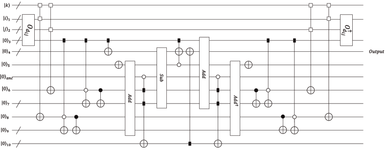
Figure 1: The first iteration process of quantum Floyd algorithm circuit diagram. The white box represents the map function to check equality, and the long black box indicates the preparation of a copy of the quantum register.

Step A8: Performing some inverse operations on Eq. (22), we get the result of the first update

$$|k\rangle\sum_{i,j=1}^{N}|i\rangle|j\rangle|d_{ij}^{(1)}\rangle,$$ (23)

where $|d_{ij}^{(1)}\rangle=\sum_{d_{ij}\leq d_{ik}+d_{kj}}|d_{ij}\rangle+\sum_{d_{ij}>d_{ik}+d_{kj}}|d_{ik}+d_{kj}\rangle$ represents the distance superposition quantum state. In short, we have achieved the following transformation:

$$\sum_{i,j=1}^{N}|i\rangle|j\rangle|d_{ij}\rangle\to\sum_{i,j=1}^{N}|i\rangle|j\rangle|d_{ij}^{(1)}\rangle.$$ (24)

We also need to be concerned that the result of the current should be the input of the next update. To make the paper more compact, in the next step we start from the initial input state at the r-th iteration.
Step A9: Initializing the input quantum state of r-th iteration process as

$$|k\rangle\sum_{i,j=1}^{N}|i\rangle|j\rangle|d_{ij}^{(r-1)}\rangle,$$ (25)

where $k$ represents the label of the transit node in the process, and the label of each update is different.
Step A10: Performing a procedure similar to the first iteration, we then obtain the geodesic distance matrix quantum state

$$\sum_{i,j=1}^{N}|i\rangle|j\rangle|d_{ij}^{(r)}\rangle,$$ (26)

where $\sum_{i,j=1}^{N}|i\rangle|j\rangle|d_{ij}^{(r)}\rangle$ is the result of quantum Floyd algorithm. Since the subsequent algorithm needs to sample, we need an extra step to transfer the information to the amplitude.
Step A11: Using the QDAC algorithm [29], we can get the quantum state

$$\frac{1}{\sqrt{G}}\sum_{i,j=1}^{N}\sqrt{d_{ij}^{(r)}}|i\rangle|j\rangle|d_{ij}^{(r)}\rangle,$$ (27)

where $G=\sum_{i,j=1}^{N}{d_{ij}^{(r)}}$. Denote the time complexity of steps $A1-A10$ as $T_{g}$, the time complexity above will be $T_{g}/P_{1}$, where $P_{1}$ represents the sum of the square of the data mean and the variance. It should be noted that applying the amplitude amplification technique [30] reduces the original time complexity of $A1-A11$ from $O(T_{g}/P_{1})$ to $O(T_{g}/\sqrt{P_{1}})$. In addition, the time complexity of this algorithm scale to $O(polylogN)$ when random sampling [31] for multi-class dataset.

III.2 Quantum Isomap algorithm based on quantum Floyd algorithm

In this section, we mainly describe the process of quantum Isomap algorithm, which is based on the quantum Floyd algorithm. The algorithm will be described in three parts as follows.

III.2.1 Constructing the geodesic distance quantum state

In Subsection A of III, we propose a quantum Floyd algorithm. In addition, the introduced quantum Floyd algorithm allows us to prepare two forms of geodesic distance quantum states. One stores the information in the quantum register, we denote it as

$$|D_{1}\rangle=\frac{1}{N}\sum_{i,j=1}^{N}|i\rangle|j\rangle|d_{ij}^{(r)}\rangle,$$ (28)

which is used as an input state for the preparation of inner product matrix quantum state. The other is stored in the amplitude of the computational basis. We donote it as

$$|D_{2}\rangle=\frac{1}{\sqrt{G}}\sum_{i,j=1}^{N}\sqrt{d_{ij}^{(r)}}|i\rangle_{1}|j\rangle_{2}{(|d_{ij}^{(r)}\rangle)}_{3},$$ (29)

where $G=\sum_{i,j=1}^{N}{d_{ij}^{(r)}}$. Note that the quantum state $|D_{2}\rangle$ is used for sampling. Both forms of quantum states allow us to prepare inner product matrix quantum state.

III.2.2 Constructing the inner product matrix quantum state

According to Eq. (3), we need to calculate the expected values of arbitrary label before preparing the inner product matrix quantum state. We have a quantum model $d_{i*}$, which computes the expectation for any label $i$, namely

$$d_{i*}=\sum_{j=1}^{N}\langle 0|U^{\dagger}{(\theta)}M_{ij}U{(\theta)}|0\rangle*(d_{ij}^{(r)}),$$ (30)

where $U{(\theta)}:|0\rangle\mapsto|D_{2}\rangle$, $M_{ij}:=|i\rangle|j\rangle\langle i|\langle j|\otimes I$ and $G$ represents a constant as shown before. Here, $|d_{i*}-d_{i*}^{(r)}|\leq\epsilon$, where $d_{i*}^{(r)}$ is the mean value corresponding to the label $i$, and $\epsilon$ is the error. The time complexity of getting each label’ expectation is about $O(T_{g}NlogN/\sqrt{P_{1}})$. This enables us to understand each entry by sampling, and then store it in QRAM structure.
Now, we begin to describe the process for preparing the inner product matrix quantum state. The steps are as follows: Step B1: appending quantum registers to the state $|D_{1}\rangle$, we will get the quantum state

$$|\phi\rangle_{1}=\frac{1}{N}\sum_{i,j=1}^{N}|i\rangle_{1}|j\rangle_{2}|d_{ij}^{(r)}\rangle_{3}|0\rangle_{4}|0\rangle_{5}|0\rangle_{6}|0\rangle_{7},$$ (31)

Step B2: Loading the expected value to the quantum register, and we will get

$$|\phi\rangle_{2}=\frac{1}{N}\sum_{i,j=1}^{N}|i\rangle_{1}|j\rangle_{2}{(|d_{ij}^{(r)}\rangle)}_{3}|d_{i*}\rangle_{4}|d_{*j}\rangle_{5}|d_{**}\rangle_{6}|0\rangle_{7},$$ (32)

Here, $d_{i*}$ and $d_{*j}$ represent the row/column mean of the geodesic distance matrix, and $d_{**}$ can be calculated by $d_{i*}$ and $d_{*j}$ without sampling. Note that the quantum states $|d_{i*}\rangle$ and $|d_{*j}\rangle$ are expressed by 2’s complement.
Step B3: Executing the quantum adder for quantum registers 3,4,5 and 6, we will the quantum state

$$|\phi\rangle_{3}=\frac{1}{N}\sum_{i,j=1}^{N}|i\rangle_{1}|j\rangle_{2}{|d_{ij}^{(r)}+d_{i*}+d_{*j}+d_{**}\rangle}_{3}|d_{i*}\rangle_{4}|d_{*j}\rangle_{5}|d_{**}\rangle_{6}|0\rangle_{7},$$ (33)

where $d_{i*}$ and $d_{*j}$ are 2’s complement of $-d_{i*}$ and $-d_{*j}$, respectively.
Step B4: Performing the shift-R operation [32] on quantum register 3, which is equivalent to multiplying 1/2. Next, we apply one $X$ gate to the quantum register 7 for the next step, the quantum state will be

$$|\phi\rangle_{4}=\frac{1}{N}\sum_{i,j=1}^{N}|i\rangle_{1}|j\rangle_{2}{|\frac{1}{2}(d_{ij}^{(r)}+d_{i*}+d_{*j}+d_{**})\rangle}_{3}|d_{i*}\rangle_{4}|d_{*j}\rangle_{5}|d_{**}\rangle_{6}|1\rangle_{7},$$ (34)

Step B5: Performing $X$ gates on quantum register 3, and then performing a quantum adder on quantum registers 3 and 7. We finally get the quantum state

$$|\phi\rangle_{5}=\frac{1}{N}\sum_{i,j=1}^{N}|i\rangle_{1}|j\rangle_{2}{|-\frac{1}{2}(d_{ij}^{(r)}+d_{i*}+d_{*j}+d_{**})\rangle}_{3}|d_{i*}\rangle_{4}|d_{*j}\rangle_{5}|d_{**}\rangle_{6}|1\rangle_{7},$$ (35)

where the quantum register 3 storing the inner product matrix information.
Step B6: Performing some inverse operations on Eq. (35), we get the result

$$|\phi\rangle_{6}=\frac{1}{N}\sum_{i,j=1}^{N}|i\rangle|j\rangle|k{(i,j)}\rangle,$$ (36)

where $k(i,j)=-\frac{1}{2}(d_{ij}^{(r)}+d_{i*}+d_{*j}+d_{**})$ rerpesents the entry of the inner product matrix.
Step B7: Executing the QDAC algorithm, which allows us prepare the state

$$|K\rangle=\frac{1}{\sqrt{C}}\sum_{i,j=1}^{N}{k(i,j)}|i\rangle|j\rangle.$$ (37)

where $C=\sum_{i,j=1}^{N}{k(i,j)}^{2}$. Let $P_{2}$ the sum of square of the data mean and variance. Combining with quantum amplifying technology, we can infer that the time complexity of preparing inner product quantum states is $O({T_{g}/\sqrt{P_{2}}})$.

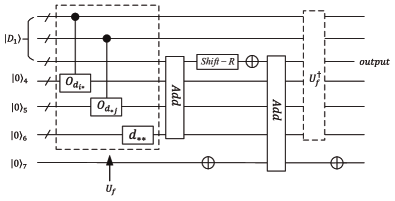
Figure 2: Preparation of inner product matrix quantum states. The black dot in $U_{f}$ controls the loading of data. In addition, Shift-R implements: $|a_{m}a_{m-1}\dots a_{2}a_{1}0\rangle\to|0a_{m}a_{m-1}\dots a_{1}\rangle$.

III.2.3 Eigensolution of the inner product matrix

The last step of the quantum isomap algorithm is to solve the eigensolution for the inner product matrix. As previously mentioned, the inner product matrix $K$ is a symmetric positive semidefinite. Let the inner product matrix $K=\sum_{k=1}^{N}\sigma_{k}|v_{k}\rangle\langle v_{k}|$, we rewrite the inner product quantum state as

$$|K\rangle=\sum_{k=1}^{N}\sigma_{k}|v_{k}\rangle|v_{k}\rangle.$$ (38)

In quantum singular value estimation of Section II, we mentioned that the ability to prepare a matrix quantum state allows us efficient prepare the unitary $U_{\mathcal{M}}$ and $U_{\mathcal{N}}$. Then, we perform quantum singular value estimation on $|K\rangle$ as the following steps:
Step C1: Appending $\lceil logN\rceil$ qubits on the state $K$, we perform the map $\mathcal{M}$ on the second register of $|K\rangle$ to obtain the state

$$|\psi\rangle_{1} =\sum_{k=1}^{N}\sigma_{k}|v_{k}\rangle\mathcal{M}|v_{k}\rangle$$ (39)

$$=\sum_{k=1}^{N}\sigma_{k}|v_{k}\rangle\sqrt{2}{(|x_{+}^{k}\rangle+|x_{-}^{k}\rangle)}$$

where $|x_{\pm}^{k}\rangle$ represents the eigenvector of the operation $W$.
Step C2: Further append some qubits, and performing the quantum phase estimation algorithm, and obtain the result

$$|\psi\rangle_{2}=\sum_{k=1}^{N}\sigma_{k}|v_{k}\rangle\sqrt{2}{(|x_{+}^{k}\rangle|\overline{\theta_{k}}\rangle+|x_{-}^{k}\rangle|-\overline{\theta_{k}}\rangle)}.$$ (40)

The size of the last quantum register depends on the accuracy $\epsilon$ of the circuit, which affects the time complexity of the quantum phase estimation algorithm.
Step C3: Using an oracle $U_{c}:|\pm\overline{\theta_{k}}\rangle|0\rangle\mapsto|\pm\overline{\theta_{k}}\rangle|cos\overline{\theta_{k}}\rangle$, which computes the eigenvalue of the inner product matrix. Storing the $cos\theta_{k}$ in the new quantum register, it leads to the state

$$|\psi\rangle_{3}=\sum_{k=1}^{N}\sigma_{k}|v_{k}\rangle\sqrt{2}{(|x_{+}^{k}\rangle|\overline{\theta_{k}}\rangle+|x_{-}^{k}\rangle|-\overline{\theta_{k}}\rangle)}|cos\overline{\theta_{k}}\rangle.$$ (41)

Note that Wang [32] gives one concrete quantum circuit to achieve the oracle $U_{c}$.
Step C4: Undo the quantum phase estimation algorithm, we then obtain

$$|\psi\rangle_{4}=\sum_{k=1}^{N}\sigma_{k}|v_{k}\rangle\mathcal{N}|v_{k}\rangle|cos\overline{\theta_{k}}\rangle.$$ (42)

Step C5: Applying the operation $\mathcal{N}^{\dagger}$, we obtain the state

$$|\psi\rangle_{5}=\sum_{k=1}^{N}\sigma_{k}|v_{k}\rangle|v_{k}\rangle|cos\overline{\theta_{k}}\rangle,$$ (43)

where $cos\overline{\theta_{k}}$ is approximates to the eigenvalue $\sigma_{k}$ with accuracy $\epsilon$.

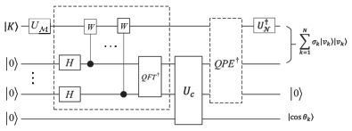
Figure 3: A simple quantum circuit describing the eigen-decomposition problem. The dashed box on the left is the unrolled representation of the quantum phase estimation circuit, and $QPE^{\dagger}$ is the inverse phase estimation. $U_{c}$ represents the quantum circuit for preparing the quantum cosine function.

Finally, we sample the state of Eq. (43) by measuring the last register to reveal the singular values $\sigma_{k}$, and the corresponding states $|v_{k}\rangle$. Apparently, we aim to select $d$ largest eigenvalues for the inner product matrix, and $\sigma_{k}$ satisfy $\sum_{k=1}^{d}\sigma_{k}^{2}/\sum_{k=1}^{N}\sigma_{k}^{2}\geq\eta\approx 1$, where $\eta$ is the threshold. Therefore, sampling the state $|\psi_{5}\rangle$ for $O(d)$ times suffices to obtain $\sigma_{k}$ and $|v_{k}\rangle$.
To understand the structure of the eigenvector, we can use vector state tomography algorithm [33]. Since each $|v_{k}\rangle$ constituted by the computational basis, this means

$$|v_{k}\rangle=\alpha_{0}|0\rangle+\alpha_{1}|1\rangle+\cdots+\alpha_{logN-1}|logN-1\rangle.$$ (44)

Measure $O(NlogN)$ copies of $|v_{k}\rangle$ in the standard basis and obtain estimates $\alpha_{i}=n_{i}/N$, where $n_{i}$ is the number of times outcomes $i$ is observed. As a result, we will get the $d$ largest eigenvalues and their corresponding eigenvectors.

IV Runtime analysis

Let us start discussing the time complexity of the whole algorithm. An overview of the time complexity of each step is listed in Table I. More detailed analysis of the algorithm is depicted as follows.
For multi-class data sets, the complexity of the quantum Floyd algorithm can be reduced to multilogarithm by using random sampling technology. In fact, we need to sample the quantum circuit before the Steps $B1-B7$. Let the complexity of steps $A1-A11$ be $O(T_{g}/\sqrt{P_{1}})$, which implies that the sample time complexity is $O(N^{2}logNT_{g}/\sqrt{P_{1}})$. Let the time complexity of $T_{g}$ be $O(polylogN)$, and $\sqrt{P_{1}}$ is independent of the dataset size $N$, the time complexity reduced to $O(N^{2}polylogN)$.
Storing each entry in QRAM data structure after sampling, which allows us efficiently prepare the inner product matrix quantum state $|D_{1}\rangle$ in subsequent step. In Fig. 2, we find that the time complexity of each step is at most $O(polylogN)$. In this way, the complexity of Steps $B1-B7$ are $O((polylogN)/\sqrt{p_{2}})$. In addition, the data structure of QRAM enables us to construct the unitary $U_{\mathcal{M}}$ and $U_{\mathcal{N}}$ with time complexity $O(polylogN)$. It should be noted that the time complexity of operator $W$ is mainly contributed by $U_{\mathcal{M}}$ and $U_{\mathcal{M}}$. This means the time complexity of steps $C1-C5$ are $O(polylogN/\epsilon\sqrt{P_{2}})$. We use the state tomography algorithm to extract the eigenvectors for $d$ largest eigenvalues. The time complexity of state tomography algorithm is $O(dNlogN)$.
In summary, the quantum Floyd algorithm can exponentially speed up classical Floyd algorithms. But, it will be $O(N^{2}polylogN)$ after sampling. In this condition, our algorithm provides substantial speed compared to the classical Floyd algorithm that runs in time $O(N^{3})$, particularly for the case of large datasets. Furthermore, putting all runtime together, our algorithm has the overall runtime $O(dNpolylogN/\epsilon\sqrt{P_{2}})$. When the $\epsilon$ and $\sqrt{P_{2}}$ are independent of the size $N$, the expected runtime reduces to $O(dNpolylogN)$. Compared with the classical time complexity $O(N^{3})$ according to Ref. [4], our algorithm produces a significant effect.

Table 1: Time complexity each step of the quantum Isomap algorithm.

Steps	Time complexity
$A1-A11$	$O(T_{g}/\sqrt{P_{1}})$
$B1-B7$	$O((T_{g}/\sqrt{P_{1}}+polylogN)/\sqrt{p_{2}})$
$C1-C5$	$O(polylogN/\epsilon\sqrt{P_{2}})$
State tomography algorithm	$O(dNpolylogN)$

V conclusions

The Isomap algorithm has many practical applications in real life. As an improvement over the classical Isomap algorithm, quantum Isomap has the significant advantage of lower time complexity. It is particularly involved in the processing of big data samples, which leads to more cost savings. The quantum Floyd algorithm mentioned in is also a highlight of our algorithm, which solves the shortest path for any two data. In our algorithm, the biggest problem in solving the eigensolution of inner product matrix is that the density matrix cannot be prepared by using the partial trace. Then, we adopt the quantum singular value estimation algorithm, which computes the eigenvalue of the inner product matrix in the new invariant subspace. Note that the algorithm relies on the binary structure of the QRAM model. Then, we can efficiently construct the operation for quantum singular value estimation. After analysis, we draw the conclusion that both two algorithms in this paper realize the acceleration of the classical algorithm. Finally, we hope that our algorithm will promote the development of quantum machine learning algorithms and enlighten more readers.

References

- Indyk and Motwani [1998] P. Indyk and R. Motwani, Approximate nearest neighbors: towards removing the curse of dimensionality, in Proceedings of the thirtieth annual ACM symposium on Theory of computing (1998) pp. 604–613.
- Ma and Zhu [2013] Y. Ma and L. Zhu, A review on dimension reduction, International Statistical Review 81, 134 (2013).
- Espadoto et al. [2019] M. Espadoto, R. M. Martins, A. Kerren, N. S. Hirata, and A. C. Telea, Toward a quantitative survey of dimension reduction techniques, IEEE transactions on visualization and computer graphics 27, 2153 (2019).
- Anowar et al. [2021] F. Anowar, S. Sadaoui, and B. Selim, Conceptual and empirical comparison of dimensionality reduction algorithms (pca, kpca, lda, mds, svd, lle, isomap, le, ica, t-sne), Computer Science Review 40, 100378 (2021).
- LaPierre [2021] R. LaPierre, Shor algorithm, in Introduction to Quantum Computing (Springer, 2021) pp. 177–192.
- Khanal et al. [2021] B. Khanal, P. Rivas, J. Orduz, and A. Zhakubayev, Quantum machine learning: A case study of grover’s algorithm, in 2021 International Conference on Computational Science and Computational Intelligence (CSCI) (IEEE, 2021) pp. 79–84.
- Alchieri et al. [2021] L. Alchieri, D. Badalotti, P. Bonardi, and S. Bianco, An introduction to quantum machine learning: from quantum logic to quantum deep learning, Quantum Machine Intelligence 3, 1 (2021).
- Massoli et al. [2022] F. V. Massoli, L. Vadicamo, G. Amato, and F. Falchi, A leap among quantum computing and quantum neural networks: A survey, ACM Computing Surveys (CSUR) (2022).
- Lloyd et al. [2014] S. Lloyd, M. Mohseni, and P. Rebentrost, Quantum principal component analysis, Nature Physics 10, 631 (2014).
- Cong and Duan [2016] I. Cong and L. Duan, Quantum discriminant analysis for dimensionality reduction and classification, New Journal of Physics 18, 073011 (2016).
- He et al. [2020] X. He, L. Sun, C. Lyu, and X. Wang, Quantum locally linear embedding for nonlinear dimensionality reduction, Quantum Information Processing 19, 1 (2020).
- Li et al. [2020] Y. Li, R.-G. Zhou, R. Xu, W. Hu, and P. Fan, Quantum algorithm for the nonlinear dimensionality reduction with arbitrary kernel, Quantum Science and Technology 6, 014001 (2020).
- Sornsaeng et al. [2021] A. Sornsaeng, N. Dangniam, P. Palittapongarnpim, and T. Chotibut, Quantum diffusion map for nonlinear dimensionality reduction, Physical Review A 104, 052410 (2021).
- Lyu et al. [2021] D. Lyu, Z. Chen, Z. Cai, and S. Piao, Robot path planning by leveraging the graph-encoded floyd algorithm, Future Generation Computer Systems 122, 204 (2021).
- Wossnig et al. [2017] L. Wossnig, Z. Zhao, and A. Prakash, Quantum linear system algorithm for dense matrices, arXiv preprint arXiv:1704.06174 (2017).
- Shao and Xiang [2018] C. Shao and H. Xiang, Quantum circulant preconditioner for a linear system of equations, Physical Review A 98, 062321 (2018).
- Szegedy [2004] M. Szegedy, Quantum speed-up of markov chain based algorithms, in 45th Annual IEEE symposium on foundations of computer science (IEEE, 2004) pp. 32–41.
- Paparo and Martin-Delgado [2012] G. D. Paparo and M. Martin-Delgado, Google in a quantum network, Scientific reports 2, 1 (2012).
- Nielsen and Chuang [2002] M. A. Nielsen and I. Chuang, Quantum computation and quantum information (2002).
- Liu et al. [2018] Y. Liu, J. Yuan, B. Duan, and D. Li, Quantum walks on regular uniform hypergraphs, Scientific reports 8, 1 (2018).
- Wu and Chan [2004] Y. Wu and K. L. Chan, An extended isomap algorithm for learning multi-class manifold, in Proceedings of 2004 International Conference on Machine Learning and Cybernetics (IEEE Cat. No. 04EX826), Vol. 6 (IEEE, 2004) pp. 3429–3433.
- Kerenidis and Landman [2021] I. Kerenidis and J. Landman, Quantum spectral clustering, Physical Review A 103, 042415 (2021).
- Takahashi et al. [2009] Y. Takahashi, S. Tani, and N. Kunihiro, Quantum addition circuits and unbounded fan-out, arXiv preprint arXiv:0910.2530 (2009).
- Gidney [2018] C. Gidney, Halving the cost of quantum addition, Quantum 2, 74 (2018).
- Thapliyal et al. [2019] H. Thapliyal, E. Munoz-Coreas, T. Varun, and T. S. Humble, Quantum circuit designs of integer division optimizing t-count and t-depth, IEEE transactions on emerging topics in computing 9, 1045 (2019).
- Wiebe et al. [2014] N. Wiebe, A. Kapoor, and K. Svore, Quantum algorithms for nearest-neighbor methods for supervised and unsupervised learning, arXiv preprint arXiv:1401.2142 (2014).
- Heidari and Farzadnia [2017] S. Heidari and E. Farzadnia, A novel quantum lsb-based steganography method using the gray code for colored quantum images, Quantum Information Processing 16, 1 (2017).
- Li et al. [2022a] J. Li, S. Lin, K. Yu, and G. Guo, Quantum k-nearest neighbor classification algorithm based on hamming distance, Quantum Information Processing 21, 1 (2022a).
- Mitarai et al. [2019] K. Mitarai, M. Kitagawa, and K. Fujii, Quantum analog-digital conversion, Physical Review A 99, 012301 (2019).
- Brassard et al. [2002] G. Brassard, P. Hoyer, M. Mosca, and A. Tapp, Quantum amplitude amplification and estimation, Contemporary Mathematics 305, 53 (2002).
- Li et al. [2022b] J. Li, S. Lin, K. Yu, and G. Guo, Quantum k-nearest neighbor classification algorithm based on hamming distance, Quantum Information Processing 21, 1 (2022b).
- Wang et al. [2020] S. Wang, Z. Wang, W. Li, L. Fan, G. Cui, Z. Wei, and Y. Gu, Quantum circuits design for evaluating transcendental functions based on a function-value binary expansion method, Quantum Information Processing 19, 1 (2020).
- Kerenidis and Prakash [2020] I. Kerenidis and A. Prakash, A quantum interior point method for lps and sdps, ACM Transactions on Quantum Computing 1, 1 (2020).