Discrete Convex Analysis:
A Tool for Economics and Game Theory

Abstract

This paper presents discrete convex analysis as a tool for economics and game theory. Discrete convex analysis is a new framework of discrete mathematics and optimization, developed during the last two decades. Recently, it is being recognized as a powerful tool for analyzing economic or game models with indivisibilities. The main feature of discrete convex analysis is the distinction of two convexity concepts, M-convexity and L-convexity, for functions in integer or binary variables, together with their conjugacy relationship. The crucial fact is that M-concavity, or its variant called M^♮-concavity, is equivalent to the (gross) substitutes property in economics. Fundamental theorems in discrete convex analysis such as the M-L conjugacy theorems, discrete separation theorems and discrete fixed point theorems yield structural results in economics such as the existence of equilibria and the lattice structure of equilibrium price vectors. Algorithms in discrete convex analysis give iterative auction algorithms as well as computational methods for equilibria.

1 Introduction

Convex analysis and fixed point theorems have played a crucial role in economic and game-theoretic analysis, for instance, to prove the existence of competitive equilibrium and Nash equilibrium; see Debreu (1959), Arrow and Hahn (1971), and Fudenberg and Tirole (1991). Traditionally, in such studies, it is assumed that commodities are perfectly divisible, or mixed strategies can be used, or the space of strategies is continuous. However, this traditional approach cannot be equally applied to economic models which involve significant indivisibilities or to game-theoretic models where the space of strategies is discrete and mixed strategies do not make much sense. In this paper we will present a new approach based on discrete convex analysis and discrete fixed point theorems, which have been recently developed in the field of discrete mathematics and optimization and become a powerful tool for analyzing economic or game models with indivisibilities.

Discrete convex analysis (Murota 1998, 2003) is a general theoretical framework constructed through a combination of convex analysis and combinatorial mathematics. The framework of convex analysis is adapted to discrete settings and the mathematical results in matroid/submodular function theory are generalized. The theory extends the direction set forth in discrete optimization around 1980 by Edmonds (1970), Frank (1982), Fujishige (1984), and Lovász (1983); see also Fujishige (2005). The main feature of discrete convex analysis is the distinction of two convexity concepts for functions in integer or binary variables, M-convexity and L-convexity, together with their conjugacy relationship with respect to the (continuous or discrete) Legendre–Fenchel transformation. Roughly speaking, M-convexity is defined in terms of an exchange property and L-convexity by submodularity.

The interaction between discrete convex analysis and mathematical economics was initiated by Danilov, Koshevoy, and Murota (1998, 2001) for the Walrasian equilibrium of indivisible markets (see also Chapter 11 of Murota 2003). The next stage of the interaction was brought about by the crucial observation of Fujishige and Yang (2003) that M-concavity, or its variant called M^♮-concavity, is equivalent to the gross substitutability (GS) of Kelso and Crawford (1982). The survey papers by Murota and Tamura (2003b) and Tamura (2004) describe the interaction at the earlier stages.

Concepts, theorems, and algorithms in discrete convex analysis have turned out to be useful in modeling and analysis of economic problems. The M-L conjugacy corresponds to the conjugacy between commodity bundles and price vectors in economics. The conjugacy theorem in discrete convex analysis implies, for example, that a valuation (utility) function has substitutes property (M^♮-concavity) if and only if the indirect utility function is an L^♮-convex function, where L^♮-convexity is a variant of L-convexity.

One of the most successful examples of the discrete convex analysis approach is Fujishige and Tamura’s model (Fujishige and Tamura 2006, 2007) of two-sided matching, which unifies the stable matching of Gale and Shapley (1962) and the assignment model of Shapley and Shubik (1972). The existence of a market equilibrium is established by revealing a novel duality-related property of M^♮-concave functions. Tamura’s monograph (Tamura 2009), though in Japanese, gives a comprehensive account of this model.

Another significant instance of the discrete convex analysis approach is the design and analysis of auction algorithms. Based on the Lyapunov function approach of Ausubel (2006), Murota, Shioura, and Yang (2013a, 2016) shed a new light on a variety of iterative auctions by making full use of the M-L conjugacy theorem and L^♮-convex function minimization algorithms. The lattice structure of equilibrium price vectors is obtained as an immediate consequence of the L^♮-convexity of the Lyapunov function.

The contents of this paper are as follows:

Section 1: Introduction
Section 2: Notation
Section 3: M^♮-concave set function
Section 4: M^♮-concave function on $\mathbb{Z}^{n}$
Section 5: M^♮-concave function on $\mathbb{R}^{n}$
Section 6: Operations for M^♮-concave functions
Section 7: Conjugacy and L^♮-convexity
Section 8: Iterative auctions
Section 9: Intersection and separation theorems
Section 10: Stable marriage and assignment game
Section 11: Valuated assignment problem
Section 12: Submodular flow problem
Section 13: Discrete fixed point theorem
Section 14: Other topics

Following the introduction of notations in Section 2, Sections 3 to 5 present the definition of M^♮-concave functions and the characterizations of (or equivalent conditions for) M^♮-concavity in terms of demand functions and choice functions. Section 6 shows the operations valid for M^♮-concave functions, including convolution operation used for the aggregation of utility functions. Section 7 introduces L^♮-convexity as the conjugate concept of M^♮-concavity, and Section 8 presents the application to iterative auctions. Section 9 deals with duality theorems of fundamental importance, including the discrete separation theorems and the Fenchel-type minimax relations. Section 10 is a succinct description of Fujishige and Tamura’s model. Combinations of M^♮-concave functions with graph/network structures are considered in Sections 11 and 12. Section 13 explains the basic idea underlying the discrete fixed point theorems. Finally in Section 14, some topics not covered in the main body of the paper are touched upon briefly.

Beside economics and game theory, discrete convex analysis has found applications in many different areas, including systems analysis (Murota 2000) in engineering, and resource allocation (Katoh et al. 2013) and inventory theory (Simchi-Levi et al. 2014) in operations research. The survey paper (Murota 2009) describes other applications including those to finite metric spaces and eigenvalues of Hermitian matrices.

2 Notation

Basic notations are listed here.

• The set of all real numbers is denoted by $\mathbb{R}$, and the sets of nonnegative reals and positive reals are denoted, respectively, by $\mathbb{R}_{+}$ and $\mathbb{R}_{++}$. The set of all integers is denoted by $\mathbb{Z}$, and the sets of nonnegative integers and positive integers are denoted, respectively, by $\mathbb{Z}_{+}$ and $\mathbb{Z}_{++}$.

• We consistently assume $N=\{1,2,\ldots,n\}$ for a positive integer $n$. Then $2^{N}$ denotes the set of all subsets of $N$, i.e., the power set of $N$.

• The characteristic vector of a subset $A\subseteq N=\{1,2,\ldots,n\}$ is denoted by $\chi_{A}\in\{0,1\}^{n}$. That is,

  $$(\chi_{A})_{i}=\left\{\begin{array}[]{ll}1&(i\in A),\\ 0&(i\in N\setminus A).\\ \end{array}\right.$$ (2.1)

  For $i\in\{1,2,\ldots,n\}$, we write $\chi_{i}$ for $\chi_{\{i\}}$, which is the $i$th unit vector. We define $\chi_{0}={\bf 0}$ where ${\bf 0}=(0,0,\ldots,0)$. We also define ${\bf 1}=(1,1,\ldots,1)$.

• For a vector $x=(x_{1},x_{2},\ldots,x_{n})$ and a subset $A\subseteq\{1,2,\ldots,n\}$, $x(A)$ denotes the component sum within $A$, i.e., $x(A)=\sum_{i\in A}x_{i}$.

• For two vectors $x=(x_{1},x_{2},\ldots,x_{n})$ and $y=(y_{1},y_{2},\ldots,y_{n})$, $x\leq y$ means the componentwise inequality. That is, $x\leq y$ is true if and only if $x_{i}\leq y_{i}$ is true for all $i=1,2,\ldots,n$.

• For two integer vectors $a$ and $b$ in $\mathbb{Z}^{n}$ with $a\leq b$, $[a,b]_{\mathbb{Z}}$ denotes the integer interval between $a$ and $b$ (inclusive), i.e., $[a,b]_{\mathbb{Z}}=\{x\in\mathbb{Z}^{n}\mid a\leq x\leq b\}$.

• For two vectors $x$ and $y$, $x\vee y$ and $x\wedge y$ denote the vectors of componentwise maximum and minimum. That is, $(x\vee y)_{i}=\max(x_{i},y_{i})$ and $(x\wedge y)_{i}=\min(x_{i},y_{i})$ for $i=1,\ldots,n$.

• For a real number $z\in\mathbb{R}$, $\left\lceil z\right\rceil$ denotes the smallest integer not smaller than $z$ (rounding-up to the nearest integer) and $\left\lfloor z\right\rfloor$ the largest integer not larger than $z$ (rounding-down to the nearest integer). This operation is extended to a vector by componentwise application.

• For a vector $x$, ${\rm supp}^{+}(x)=\{i\mid x_{i}>0\}$ and ${\rm supp}^{-}(x)=\{i\mid x_{i}<0\}$ denote the positive and negative supports of $x$, respectively.

• The $\ell_{\infty}$-norm of a vector $x$ is denoted as $\|x\|_{\infty}$, i.e., $\|x\|_{\infty}=\max(|x_{1}|,|x_{2}|,\ldots,|x_{n}|)$. Variants are: $\|x\|_{\infty}^{+}=\max(0,x_{1},x_{2},\ldots,x_{n})$ and $\|x\|_{\infty}^{-}=\max(0,-x_{1},-x_{2},\ldots,-x_{n})$.

• For two vectors $p=(p_{1},p_{2},\ldots,p_{n})$ and $x=(x_{1},x_{2},\ldots,x_{n})$, their inner product is denoted by $\langle p,x\rangle$, i.e., $\langle p,x\rangle=p^{\top}x=\sum_{i=1}^{n}p_{i}x_{i}$, where $p^{\top}$ is the transpose of $p$ viewed as a column vector.

• For a function $f:\mathbb{R}^{n}\to\mathbb{R}\cup\{+\infty\}$ or $f:\mathbb{R}^{n}\to\mathbb{R}\cup\{-\infty\}$,

  $${\rm dom\,}f = \{x\mid-\infty<f(x)<+\infty\},$$

  $$\arg\min f = \{x\mid f(x)\leq f(y)\ \ \mbox{for all $y$}\,\},$$

  $$\arg\max f = \{x\mid f(x)\geq f(y)\ \ \mbox{for all $y$}\,\}.$$

  These notations are used also for $f:\mathbb{Z}^{n}\to\mathbb{R}\cup\{+\infty\}$ or $f:\mathbb{Z}^{n}\to\mathbb{R}\cup\{-\infty\}$. We sometimes use ${\rm dom_{\mathbb{R}}}f$ and ${\rm dom_{\mathbb{Z}}}f$ to emphasize that ${\rm dom\,}f\subseteq\mathbb{R}^{n}$ and ${\rm dom\,}f\subseteq\mathbb{Z}^{n}$.

• For a set function $f:2^{N}\to\mathbb{R}\cup\{+\infty\}$ or $f:2^{N}\to\mathbb{R}\cup\{-\infty\}$,

  $${\rm dom\,}f = \{X\subseteq N\mid-\infty<f(X)<+\infty\},$$

  $$\arg\min f = \{X\subseteq N\mid f(X)\leq f(Y)\ \ \mbox{for all $Y\subseteq N$}\,\},$$

  $$\arg\max f = \{X\subseteq N\mid f(X)\geq f(Y)\ \ \mbox{for all $Y\subseteq N$}\,\}.$$

• For a function $f$ and a vector $p$, $f[-p]$ means the function defined by

  $$f[-p](x) =f(x)-p^{\top}x=f(x)-\langle p,x\rangle.$$

  If $f$ is a set function, $f[-p]$ is the set function defined by $f[-p](X)=f(X)-p(X)$.

• For a function $f$, four variants of the conjugate function of $f$ are denoted as

  $$f^{\bullet}(p) =\sup\{\langle p,x\rangle-f(x)\},\qquad f^{\circ}(p)=\inf\{\langle p,x\rangle-f(x)\},$$

  $$f^{\triangledown}(p) =\sup\{f(x)-\langle p,x\rangle\},\qquad f^{\triangle}(p)=\inf\{f(x)+\langle p,x\rangle\}.$$

• The convex closure of a function $f$ is denoted by $\overline{f}$. The convex hull of a set $S$ is denoted by $\overline{S}$.

• $D(p;f)$ denotes the demand correspondence for a price vector $p$ and a valuation function $f$, defined in (3.16) and (4.21).

• $C(\cdot)$ denotes a choice function. $C(\cdot\,;f)$ denotes the choice function determined by a valuation function $f$, defined in (3.17) and (4.23).

• $\mathrm{tw}(\cdot)$ denotes the twisting of a set or a vector, defined in (3.18) and (4.25), respectively.

• For an arc $a$ in a directed graph, $\partial^{+}a$ denotes the initial (tail) vertex of $a$, and $\partial^{-}a$ the terminal (head) vertex of $a$. That is, $\partial^{+}a=u$ and $\partial^{-}a=v$ if $a=(u,v)$.

• For a flow $\xi$ in a network, $\partial\xi$ denotes the boundary vector on the vertex set, defined in (4.36). For a matching $M$, $\partial M$ denotes the set of the vertices incident to some edge in $M$.

• For a potential $p$ defined on the vertex set of a network, $\delta p$ denotes the coboundary of $p$, the vector on the arc set defined in (12.20).

3 M^♮-concave Set Function

First we introduce M^♮-concavity for set functions. Let $N$ be a finite set, say, $N=\{1,2,\ldots,n\}$, $\mathcal{F}$ be a nonempty family of subsets of $N$, and $f:\mathcal{F}\to\mathbb{R}$ be a real-valued function on $\mathcal{F}$. In economic applications, we may think of $f$ as a single-unit valuation (binary valuation) over combinations of indivisible commodities $N$, where $\mathcal{F}$ represents the set of feasible combinations.

3.1 Exchange property

Let $\mathcal{F}$ be a nonempty family of subsets of a finite set $N=\{1,2,\ldots,n\}$. We say that a function $f:\mathcal{F}\to\mathbb{R}$ is M^♮-concave, if, for any $X,Y\in\mathcal{F}$ and $i\in X\setminus Y$, we have (i) $X-i\in\mathcal{F}$, $Y+i\in\mathcal{F}$ and

$$f(X)+f(Y)\leq f(X-i)+f(Y+i),$$ (3.1)

or (ii) there exists some $j\in Y\setminus X$ such that $X-i+j\in\mathcal{F}$, $Y+i-j\in\mathcal{F}$ and

$$f(X)+f(Y)\leq f(X-i+j)+f(Y+i-j).$$ (3.2)

Here we use short-hand notations $X-i=X\setminus\{i\}$, $Y+i=Y\cup\{i\}$, $X-i+j=(X\setminus\{i\})\cup\{j\}$, and $Y+i-j=(Y\cup\{i\})\setminus\{j\}$. This property is referred to as the exchange property.

A more compact way of defining M^♮-concavity, free from explicit reference to the domain $\mathcal{F}$, is to define a function $f:2^{N}\to\mathbb{R}\cup\{-\infty\}$ to be M^♮-concave if it has the following property:

(M^♮-EXC)

For any $X,Y\subseteq N$ and $i\in X\setminus Y$, we have

$$f(X)+f(Y) \leq\max\left(f(X-i)+f(Y+i),\ \max_{j\in Y\setminus X}\{f(X-i+j)+f(Y+i-j)\}\right),$$ (3.3)

where $(-\infty)+a=a+(-\infty)=(-\infty)+(-\infty)=-\infty$ for $a\in\mathbb{R}$, $-\infty\leq-\infty$, and a maximum taken over an empty set is defined to be $-\infty$. The family of subsets $X$ for which $f(X)$ is finite is called the effective domain of $f$, and denoted as ${\rm dom\,}f$, i.e., ${\rm dom\,}f=\{X\mid f(X)>-\infty\}$. When $f$ is regarded as a function on $\mathcal{F}={\rm dom\,}f$, it is an M^♮-concave function in the original sense.

As a (seemingly) stronger condition than (M^♮-EXC) we may also conceive the multiple exchange property:

(M^♮-EXC_m)

For any $X,Y\subseteq N$ and $I\subseteq X\setminus Y$, there exists $J\subseteq Y\setminus X$ such that $f(X)+f(Y)\leq f((X\setminus I)\cup J)+f((Y\setminus J)\cup I)$, i.e.,

$$f(X)+f(Y)\leq\max_{J\subseteq Y\setminus X}\{f((X\setminus I)\cup J)+f((Y\setminus J)\cup I)\}.$$ (3.4)

Recently it has been shown (Murota 2018) that (M^♮-EXC_m) is equivalent to (M^♮-EXC).

Theorem 3.1.

A function $f:2^{N}\to\mathbb{R}\cup\{-\infty\}$ satisfies (M^♮-EXC) if and only if it satisfies (M^♮-EXC_m). Hence, every M^♮-concave function has the multiple exchange property (M^♮-EXC_m).

Remark 3.1.

The multiple exchange property (M^♮-EXC_m) here is the same as the “strong no complementarities property (SNC)” introduced by Gul and Stacchetti (1999), where it is shown that (SNC) implies the gross substitutes property (GS). On the other hand, (GS) is known (Fujishige and Yang 2003) to be equivalent to (M^♮-EXC) (see Theorem 3.7). Therefore, Theorem 3.1 above reveals that (SNC) is equivalent to (GS). This settles the question since 1999: Is (SNC) strictly stronger than (GS) or not? We now know that (SNC) is equivalent to (GS). See Murota (2018) for details.  

It follows from the definition of an M^♮-concave function that the (effective) domain $\mathcal{F}$ of an M^♮-concave function has the following exchange property:

(B^♮-EXC)

For any $X,Y\in\mathcal{F}$ and $i\in X\setminus Y$,  we have (i) $X-i\in\mathcal{F}$, $Y+i\in\mathcal{F}$  or  
(ii) there exists some $j\in Y\setminus X$ such that $X-i+j\in\mathcal{F}$, $Y+i-j\in\mathcal{F}$.

This means that $\mathcal{F}$ forms a matroid-like structure, called a generalized matroid (g-matroid), or an M^♮-convex family. An M^♮-convex family $\mathcal{F}$ containing the empty set forms the family of independent sets of a matroid. For example, for integers $a,b$ with $0\leq a\leq b\leq n$, $\mathcal{F}_{ab}=\{X\mid a\leq|X|\leq b\}$ is an M^♮-convex family, and $\mathcal{F}_{0b}$ (with $a=0$) forms the family of independent sets of a matroid.

Remark 3.2.

It follows from Theorem 3.1 that a nonempty family $\mathcal{F}\subseteq 2^{N}$ satisfies (B^♮-EXC) if and only if it satisfies the multiple exchange axiom:

(B^♮-EXC_m)

For any $X,Y\in\mathcal{F}$ and $I\subseteq X\setminus Y$, there exists $J\subseteq Y\setminus X$ such that $(X\setminus I)\cup J\in\mathcal{F}$ and $(Y\setminus J)\cup I\in\mathcal{F}$.  

M^♮-concavity can be characterized by a local exchange property under the assumption that function $f$ is (effectively) defined on an M^♮-convex family of sets (Murota 1996c, 2003; Murota and Shioura 1999). The conditions (3.5)–(3.7) below are “local” in the sense that they require the exchangeability of the form of (3.3) only for $(X,Y)$ with $\max(|X\setminus Y|,|Y\setminus X|)\leq 2$.

Theorem 3.2.

A set function $f:2^{N}\to\mathbb{R}\cup\{-\infty\}$ is M^♮-concave if and only if ${\rm dom\,}f$ is an M^♮-convex family and the following three conditions hold:

$$f(X+i+j)+f(X)\leq f(X+i)+f(X+j)\qquad(\forall X\subseteq N,\ \forall i,j\in N\setminus X,\ i\not=j),$$ (3.5)

$$f(X+i+j)+f(X+k)\leq\max\left[f(X+i+k)+f(X+j),f(X+j+k)+f(X+i)\right]$$

$$\hskip 216.81pt(\forall X\subseteq N,\ \forall i,j,k\,\mbox{\rm(distinct})\in N\setminus X),$$ (3.6)

$$f(X+i+j)+f(X+k+l)\leq\max\left[f(X+i+k)+f(X+j+l),f(X+j+k)+f(X+i+l)\right]$$

$$\hskip 216.81pt(\forall X\subseteq N,\ \forall i,j,k,l\,\mbox{\rm(distinct})\in N\setminus X).$$ (3.7)

When the effective domain ${\rm dom\,}f$ contains the emptyset, the local exchange condition for M^♮-concavity takes a simpler form without involving (3.7) (Reijnierse et al. 2002, Müller 2006, Shioura and Tamura 2015).

Theorem 3.3.

Let $f:2^{N}\to\mathbb{R}\cup\{-\infty\}$ be a set function such that ${\rm dom\,}f$ is an M^♮-convex family containing $\emptyset$ (the empty set). Then $f$ is M^♮-concave if and only if (3.5) and (3.6) hold.

It is known (Theorem 6.19 of Murota 2003) that an M^♮-concave function is submodular, i.e.,

$$f(X)+f(Y)\geq f(X\cup Y)+f(X\cap Y)\qquad(X,Y\subseteq N).$$ (3.8)

More precisely, the condition (3.5) above is equivalent to the submodularity (3.8) as long as ${\rm dom\,}f$ is M^♮-convex (Proposition 6.1 of Shioura and Tamura 2015).

Because of the additional condition (3.6) for M^♮-concavity, not every submodular set function is M^♮-concave. Thus, M^♮-concave set functions form a proper subclass of submodular set functions.

Remark 3.3.

It follows from (M^♮-EXC) that M^♮-concave set functions enjoy the following exchange properties under cardinality constraints (Lemmas 4.3 and 4.6 of Murota and Shioura 1999):
$\bullet$ For any $X,Y\subseteq N$ with $|X|<|Y|$,

$$f(X)+f(Y) \leq\max_{j\in Y\setminus X}\{f(X+j)+f(Y-j)\}.$$ (3.9)

$\bullet$ For any $X,Y\subseteq N$ with $|X|=|Y|$ and $i\in X\setminus Y$,

$$f(X)+f(Y) \leq\max_{j\in Y\setminus X}\{f(X-i+j)+f(Y+i-j)\}.$$ (3.10)

The former property, in particular, implies the cardinal-monotonicity of the induced choice function; see Theorem 3.10 and its proof.  

Remark 3.4.

For a set family $\mathcal{F}$ consisting of equi-cardinal sets (i.e., $|X|=|Y|$ for all $X,Y\in\mathcal{F}$) the exchange property (B^♮-EXC) takes a simpler form: For any $X,Y\in\mathcal{F}$ and $i\in X\setminus Y$, there exists some $j\in Y\setminus X$ such that $X-i+j\in\mathcal{F}$, $Y+i-j\in\mathcal{F}$. This means that $\mathcal{F}$ forms the family of bases of a matroid. An M^♮-concave function defined on matroid bases is called a valuated matroid (Dress and Wenzel 1990,1992; Chapter 5 of Murota 2000a), or an M-concave set function (Murota 1996c, 2003). The exchange property for M-concavity reads: A set function $f$ is M-concave if and only if (3.10) holds for any $X,Y\subseteq N$ and $i\in X\setminus Y$. A corollary of Theorem 3.1: Every M-concave function (valuated matroid) $f$ has the multiple exchange property (M^♮-EXC_m) with $|J|=|I|$. A further corollary of this fact is a classical result in matroid theory: The base family of a matroid has the multiple exchange property (B^♮-EXC_m) with $|J|=|I|$; see, e.g., Section 39.9a of Schrijver (2003).  

3.2 Maximization and single improvement property

For an M^♮-concave function, the maximality of a function value is characterized by a local condition (Theorem 6.26 of Murota 2003).

Theorem 3.4.

Let $f:2^{N}\to\mathbb{R}\cup\{-\infty\}$ be an M^♮-concave function and $X\in{\rm dom\,}f$. Then $X$ is a maximizer of $f$ if and only if

$$f(X) \geq f(X-i+j)\quad(\forall\,i\in X,\ \forall\,j\in N\setminus X),$$ (3.11)

$$f(X) \geq f(X-i)\qquad\ \ (\forall\,i\in X),$$ (3.12)

$$f(X) \geq f(X+j)\qquad\ \ (\forall\,j\in N\setminus X).$$ (3.13)

As a discrete analogue of the subgradient inequality for convex functions, we have the inequality (3.14) in the following theorem.

Theorem 3.5.

Let $f:2^{N}\to\mathbb{R}\cup\{-\infty\}$ be an M^♮-concave function and $X,Y\in{\rm dom\,}f$. Then

$$f(Y)-f(X)\leq\hat{f}(X,Y),$$ (3.14)

where $\hat{f}(X,Y)$ is defined as follows:

• When $|X|=|Y|$,

  $$\hat{f}(X,Y)=\max_{\sigma}\bigg{(}\sum_{i\in X\setminus Y}[f(X-i+\sigma(i))-f(X)]\bigg{)},$$

  where the maximum is taken over all one-to-one correspondences $\sigma:X\setminus Y\to Y\setminus X$.

• When $|X|<|Y|$,

  $$\hat{f}(X,Y)=\max_{\sigma}\bigg{(}\sum_{i\in X\setminus Y}[f(X-i+\sigma(i))-f(X)]+\sum_{j\in Y\setminus(X\cup\sigma(X))}[f(X+j)-f(X)]\bigg{)},$$

  where the maximum is taken over all injections $\sigma:X\setminus Y\to Y\setminus X$.

• When $|X|>|Y|$,

  $$\hat{f}(X,Y)=\max_{\tau}\bigg{(}\sum_{j\in Y\setminus X}[f(X-\tau(j)+j)-f(X)]+\sum_{i\in X\setminus(Y\cup\tau(Y))}[f(X-i)-f(X)]\bigg{)},$$

  where the maximum is taken over all injections $\tau:Y\setminus X\to X\setminus Y$.

For a vector $p=(p_{i}\mid i\in N)\in\mathbb{R}^{N}$ we use the notation $f[-p]$ to mean the function $f(X)-p(X)$, where $X\subseteq N$ and $p(X)=\sum_{i\in X}p_{i}$. That is,

$$f[-p](X)=f(X)-p(X)\qquad(X\subseteq N).$$ (3.15)

Note that $f[-p]$ is M^♮-concave if and only if $f$ is M^♮-concave.

The “if” part of Theorem 3.4, which is the content of the theorem, can be restated as follows: If $X$ is not a maximizer of $f$, there exists $Y\subseteq N$ such that $|X\setminus Y|\leq 1$, $|Y\setminus X|\leq 1$, and $f(X)<f(Y)$. By considering this property for $f[-p]$ with varying $p$, we are naturally led to the single improvement property of Gul and Stacchetti (1999):

(SI)

For any $p\in\mathbb{R}^{N}$, if $X$ is not a maximizer of $f[-p]$, there exists $Y\subseteq N$ such that $|X\setminus Y|\leq 1$, $|Y\setminus X|\leq 1$, and $f[-p](X)<f[-p](Y)$.

The above argument shows that (SI) is true for M^♮-concave functions. In fact, (SI) is equivalent to M^♮-concavity (Fujishige and Yang 2003).

3.3 Maximizers and gross substitutability

For a vector $p=(p_{i}\mid i\in N)\in\mathbb{R}^{N}$ we consider the maximizers of the function $f[-p](X)=f(X)-p(X)$, where $p(X)=\sum_{i\in X}p_{i}$ for $X\subseteq N$. We denote the set of these maximizers by

$$D(p;f)=\arg\max_{X}\{f(X)-p(X)\mid X\subseteq N\}.$$ (3.16)

In economic applications, $p$ is a price vector and $D(p)=D(p;f)$ represents the demand correspondence.

It is one of the most fundamental facts in discrete convex analysis that the M^♮-concavity of a function is characterized in terms of the M^♮-convexity of its maximizers (Murota 1996c; Theorem 6.30 of Murota 2003; Murota and Shioura 1999).

Theorem 3.6.

A set function $f:2^{N}\to\mathbb{R}\cup\{-\infty\}$ is M^♮-concave if and only if, for every vector $p\in\mathbb{R}^{N}$, $D(p;f)$ is an M^♮-convex family. That is, $f$ satisfies (M^♮-EXC) if and only if, for every $p\in\mathbb{R}^{N}$, $D(p;f)$ satisfies (B^♮-EXC).

The following are two versions of the multiple exchange property of $D(p;f)$:

(NC)

For any $p\in\mathbb{R}^{N}$, if $X,Y\in D(p;f)$ and $I\subseteq X\setminus Y$, there exists $J\subseteq Y\setminus X$ such that $(X\setminus I)\cup J\in D(p;f)$,

(NCsim)

For any $p\in\mathbb{R}^{N}$, if $X,Y\in D(p;f)$ and $I\subseteq X\setminus Y$, there exists $J\subseteq Y\setminus X$ such that $(X\setminus I)\cup J\in D(p;f)$ and $(Y\setminus J)\cup I\in D(p;f)$.

The condition (NC), introduced by Gul and Stacchetti (1999), is called “no complementarities property” and (NCsim) is a simultaneous (or symmetric) version of (NC) introduced by Murota (2018). These conditions, (NC) and (NCsim), are equivalent to each other, and are equivalent to the M^♮-concavity of $f$; see Remark 3.1 as well as (Murota 2018) for details.

In the above we have looked at the family $D(p;f)$ of the maximizers for each $p\in\mathbb{R}^{N}$. We now investigate how $D(p;f)$ changes with the variation of $p$.

A set function (single-unit valuation function) $f:2^{N}\to\mathbb{R}\cup\{-\infty\}$ is said to have the gross substitutes property if

(GS)

For any $p,q\in\mathbb{R}^{N}$ with $p\leq q$ and $X\in D(p;f)$, there exists $Y\in D(q;f)$ such that $\{i\in X\mid p_{i}=q_{i}\}\subseteq Y$.

The concept of gross substitutes property, introduced by Kelso and Crawford (1982), has turned out to be crucial in economics; see, e.g., Roth and Sotomayor (1990), Bikhchandani and Mamer (1997), Gul and Stacchetti (1999), Ausubel and Milgrom (2002), Milgrom (2004), Hatfield and Milgrom (2005), Ausubel (2006), Sun and Yang (2006), Milgrom and Strulovici (2009), and Hatfield et al. (2019).

The following theorem, due to Fujishige and Yang (2003), plays the key role to connect discrete convex analysis and economics.

Theorem 3.7.

A set function $f:2^{N}\to\mathbb{R}\cup\{-\infty\}$ has the gross substitutes property (GS) if and only if it is M^♮-concave.

It is known (Hatfield and Milgrom 2005, Milgrom and Strulovici 2009) that the gross substitutes property, and hence M^♮-concavity, implies the law of aggregate demand in the following form:

(LAD)

For any $p,q\in\mathbb{R}^{N}$ with $p\leq q$ and $X\in D(p;f)$, there exists $Y\in D(q;f)$ such that $|X|\geq|Y|$.

Gross substitutes properties for multi-unit valuations are treated in Section 4.3.

3.4 Choice function

A function $C:2^{N}\to 2^{N}$ is called a choice function if $C(Z)\subseteq Z$ for all $Z\subseteq N$. We have $C(\emptyset)=\emptyset$ and, possibly, $C(Z)=\emptyset$ for some nonempty subsets $Z$. A choice function $C$ is said to be consistent if $C(X)\subseteq Y\subseteq X$ implies $C(Y)=C(X)$. Here we discuss two other properties of choice functions, substitutability and cardinal monotonicity, which are closely related to M^♮-concavity.

The substitutability of a choice function $C$ means the following property (Roth 1984, Roth and Sotomayor 1990):

(SC_ch)

For any $Z_{1},Z_{2}\subseteq N$ with $Z_{1}\supseteq Z_{2}$ it holds that $Z_{2}\cap C(Z_{1})\subseteq C(Z_{2})$.

Several apparently different formulations of substitutability, each equivalent to (SC_ch), are found in the literature:

• For any $Z_{1},Z_{2}\subseteq N$ with $Z_{1}\supseteq Z_{2}$ it holds that $Z_{1}\setminus C(Z_{1})\supseteq Z_{2}\setminus C(Z_{2})$.

• $i\in C(X)$ implies $i\in C(Y\cup\{i\})$ for $Y\subseteq X$.

• For any $X\subseteq N$ and any distinct $i,j\in X$,  $i\in C(X)$ implies $i\in C(X\setminus\{j\})$.

A choice function $C$ is said to be cardinal-monotone if $|C(Y)|\leq|C(X)|$ for all $Y\subseteq X$ . This property is called increasing property by Fleiner (2003) and law of aggregate demand by Hatfield and Milgrom (2005).

Remark 3.5.

As is well known, consistency and substitutability together are equivalent to path independence of Plott (1973), which is characterized by the condition: $C(C(X)\cup Y)=C(X\cup Y)$ for all $X,Y\subseteq N$. This condition is equivalent to: $C(C(X)\cup C(Y))=C(X\cup Y)$ for all $X,Y\subseteq N$.  

Remark 3.6.

The above-mentioned properties of choice functions are well-known key properties in economics and game theory. In the stable matching problem, for example, consistency and substitutability (i.e., path independence) guarantee, roughly, the existence of a stable matching. If, in addition, the choice functions are cardinal-monotone, then the stable matchings form a nice lattice (with simple lattice operations, being distributive, etc.). To quote Theorem 10 of Alkan (2002): “The set of stable matchings in any two-sided market with path-independent cardinal-monotone choice functions is a distributive lattice under the common preferences of all agents on one side of the market. The supremum (infimum) operation of the lattice for each side consists componentwise of the join (meet) operation in the revealed preference ordering of associated agents. The lattice has the polarity, unicardinality and complementarity properties.”  

Remark 3.7.

A function $C:2^{N}\to 2^{N}$ is called comonotone if there exists a monotone function $g:2^{N}\to 2^{N}$ such that $C(X)=X\setminus g(X)$ for all $X\subseteq N$ (Fleiner 2003). A function $C:2^{N}\to 2^{N}$ is comonotone if and only if $C$ is a choice function with substitutability. The fixed point approach to stable matchings of Fleiner (2003) is based on the observation that stable matchings correspond to fixed points of a certain monotone function associated with the choice functions and the deferred acceptance algorithm of Gale and Shapley (1962) can be regarded as an iteration of this function. See also Farooq et al. (2012).  

A choice correspondence means a function $C:2^{N}\to 2^{2^{N}}$ such that $\emptyset\not=C(Z)\subseteq 2^{Z}$ for all $Z\subseteq N$. It should be clear that the value $C(Z)$ is not a subset of $N$ but a family of subsets of $N$. If $C(Z)$ consists of a single subset for each $Z\subseteq N$, then $C$ can be identified with a choice function $C:2^{N}\to 2^{N}$.

The substitutability of a choice correspondence $C$ is formulated as follows (Definition 4 of Sotomayor 1999):

(SC${}_{\rm ch}^{1}$)

For any $Z_{1},Z_{2}\subseteq N$ with $Z_{1}\supseteq Z_{2}$ and any $X_{1}\in C(Z_{1})$, there exists $X_{2}\in C(Z_{2})$ such that $Z_{2}\cap X_{1}\subseteq X_{2}$.

(SC${}_{\rm ch}^{2}$)

For any $Z_{1},Z_{2}\subseteq N$ with $Z_{1}\supseteq Z_{2}$ and any $X_{2}\in C(Z_{2})$, there exists $X_{1}\in C(Z_{1})$ such that $Z_{2}\cap X_{1}\subseteq X_{2}$.

For a choice function $C:2^{N}\to 2^{N}$, (SC${}_{\rm ch}^{1}$) and (SC${}_{\rm ch}^{2}$) are each equivalent to (SC_ch).

Choice function induced from a valuation function:

A valuation function $f:2^{N}\to\mathbb{R}\cup\{-\infty\}$ with $\emptyset\in{\rm dom\,}f$ induces a choice correspondence $C:2^{N}\to 2^{2^{N}}$ by

$$C(Z)=C(Z;f)=\arg\max\{f(Y)\mid Y\subseteq Z\}.$$ (3.17)

The assumption “$\emptyset\in{\rm dom\,}f$” ensures that $C(Z;f)\not=\emptyset$ for every $Z\subseteq N$. In general, the maximizer is not unique, and accordingly, $C$ is a choice correspondence (i.e., $C(Z;f)$ is a family of subsets of $N$).

While (SC${}_{\rm ch}^{1}$) and (SC${}_{\rm ch}^{2}$) above formulate the substitutability for a choice correspondence, (SC¹) and (SC²) below are the corresponding conditions for a valuation function $f$. That is, a valuation function $f$ satisfies (SC¹) if and only if the induced choice correspondence $C(\,\cdot\,;f)$ satisfies (SC${}_{\rm ch}^{1}$), and similarly for (SC²) and (SC${}_{\rm ch}^{2}$).

(SC¹)

For any $Z_{1},Z_{2}\subseteq N$ with $Z_{1}\supseteq Z_{2}$ and any $X_{1}\in C(Z_{1};f)$, there exists $X_{2}\in C(Z_{2};f)$ such that $Z_{2}\cap X_{1}\subseteq X_{2}$.

(SC²)

For any $Z_{1},Z_{2}\subseteq N$ with $Z_{1}\supseteq Z_{2}$ and any $X_{2}\in C(Z_{2};f)$, there exists $X_{1}\in C(Z_{1};f)$ such that $Z_{2}\cap X_{1}\subseteq X_{2}$.

These two conditions are independent of each other; see Examples 3.1 and 3.2 in Farooq and Tamura (2004).

A connection to M^♮-concavity is pointed out by Eguchi et al. (2003); see also Fujishige and Tamura (2006). This is another important finding, on top of Theorem 3.7 (equivalence of M^♮-concavity to (GS)), which has reinforced the connection between discrete convex analysis and economics.

Theorem 3.8.

Every M^♮-concave function $f:2^{N}\to\mathbb{R}\cup\{-\infty\}$ with $\emptyset\in{\rm dom\,}f$ satisfies (SC¹) and (SC²). That is, the choice correspondence induced from an M^♮-concave set function has the substitutability properties (SC${}_{\rm ch}^{1}$) and (SC${}_{\rm ch}^{2}$).

Proof.

Assume $Z_{1}\supseteq Z_{2}$.

Proof of (SC¹): Let $X_{1}\in C(Z_{1};f)$ and take $X_{2}\in C(Z_{2};f)$ with minimum $|(Z_{2}\cap X_{1})\setminus X_{2}|$. To prove by contradiction, suppose that there exists $i\in(Z_{2}\cap X_{1})\setminus X_{2}$. Since $i\in X_{1}\setminus X_{2}$, (M^♮-EXC) implies (i) $f(X_{1})+f(X_{2})\leq f(X_{1}-i)+f(X_{2}+i)$ or (ii) there exists $j\in X_{2}\setminus X_{1}$ such that $f(X_{1})+f(X_{2})\leq f(X_{1}-i+j)+f(X_{2}+i-j)$. In case (i) we note $X_{1}-i\subseteq Z_{1}$ and $X_{2}+i\subseteq Z_{2}$, from which follow $f(X_{1}-i)\leq f(X_{1})$ and $f(X_{2}+i)\leq f(X_{2})$. Therefore, the inequalities are in fact equalities, and $X_{1}-i\in C(Z_{1};f)$ and $X_{2}+i\in C(Z_{2};f)$. But we have $|(Z_{2}\cap X_{1})\setminus(X_{2}+i)|=|(Z_{2}\cap X_{1})\setminus X_{2}|-1$, which contradicts the choice of $X_{2}$. In case (ii) we note $X_{1}-i+j\subseteq Z_{1}$ and $X_{2}+i-j\subseteq Z_{2}$, from which follow $f(X_{1}-i+j)\leq f(X_{1})$ and $f(X_{2}+i-j)\leq f(X_{2})$. Therefore, the inequalities are in fact equalities, and $X_{1}-i+j\in C(Z_{1};f)$ and $X_{2}+i-j\in C(Z_{2};f)$. But we have $|(Z_{2}\cap X_{1})\setminus(X_{2}+i-j)|=|(Z_{2}\cap X_{1})\setminus X_{2}|-1$, which contradicts the choice of $X_{2}$.

Proof of (SC²): Let $X_{2}\in C(Z_{2};f)$ and take $X_{1}\in C(Z_{1};f)$ with minimum $|(Z_{2}\cap X_{1})\setminus X_{2}|$. By the same argument as above we obtain (i) $X_{1}-i\in C(Z_{1};f)$ with $|(Z_{2}\cap(X_{1}-i))\setminus X_{2}|=|(Z_{2}\cap X_{1})\setminus X_{2}|-1$, or (ii) $X_{1}-i+j\in C(Z_{1};f)$ with $|(Z_{2}\cap(X_{1}-i+j))\setminus X_{2}|=|(Z_{2}\cap X_{1})\setminus X_{2}|-1$. This is a contradiction to the choice of $X_{1}$. ∎

When the maximizer is unique in (3.17) for every $Z$, we say that $f$ is unique-selecting. In this case, $C$ in (3.17) is a choice function (i.e., $C(Z;f)$ is a subset of $N$ for every $Z$), and (SC¹) and (SC²) both reduce to the following condition:

(SC)

For any $Z_{1},Z_{2}\subseteq N$ with $Z_{1}\supseteq Z_{2}$ it holds that $Z_{2}\cap C(Z_{1};f)\subseteq C(Z_{2};f)$.

Theorem 3.8 yields, as a corollary, the following result of Eguchi and Fujishige (2002).

Theorem 3.9.

Every unique-selecting M^♮-concave function $f:2^{N}\to\mathbb{R}\cup\{-\infty\}$ with $\emptyset\in{\rm dom\,}f$ satisfies (SC). That is, the choice function induced from a unique-selecting M^♮-concave set function has the substitutability property (SC_ch).

Unique-selecting M^♮-concave functions are well-behaved also with respect to cardinal monotonicity. The following is a special case of Lemma 4.5 of Murota and Yokoi (2015).

Theorem 3.10.

Every unique-selecting M^♮-concave function $f:2^{N}\to\mathbb{R}\cup\{-\infty\}$ with $\emptyset\in{\rm dom\,}f$ induces a choice function with cardinal monotonicity.

Proof.

The proof is based on the exchange property (3.9) in Remark 3.3. To prove by contradiction, suppose that there exist $X$ and $Y$ such that $X\supseteq Y$ and $|C(X)|<|C(Y)|$. Set $X^{*}=C(X)$ and $Y^{*}=C(Y)$. Then $|X^{*}|<|Y^{*}|$. By the exchange property (3.9) there exists $j\in Y^{*}\setminus X^{*}$ such that $f(X^{*})+f(Y^{*})\leq f(X^{*}+j)+f(Y^{*}-j)$. Here we have $f(X^{*}+j)<f(X^{*})$ since $X^{*}+j\subseteq X$ and $X^{*}$ is the unique maximizer, and also $f(Y^{*}-j)<f(Y^{*})$ since $Y^{*}-j\subseteq Y$ and $Y^{*}$ is the unique maximizer. This is a contradiction. ∎

Thus, M^♮-concave valuation functions entail the three desirable properties. Recall Remark 3.6 for the implications of this fact.

Theorem 3.11.

The choice function induced from a unique-selecting M^♮-concave set function $f$ with $\emptyset\in{\rm dom\,}f$ has consistency, substitutability, and cardinal monotonicity.

Finally, we mention a theorem that characterizes M^♮-concavity in terms of a parametrized version of (SC¹) and (SC²). Recall from (3.15) the notation $f[-p](X)=f(X)-p(X)$ for $p\in\mathbb{R}^{N}$ and $X\subseteq N$. If $f$ is an M^♮-concave function (not assumed to be unique-selecting), $f[-p]$ is also M^♮-concave, and hence is equipped with the properties (SC¹) and (SC²) by Theorem 3.8. In other words, an M^♮-concave function $f$ has the following properties.

(SC${}^{1}_{\rm\bf{G}}$)

For any $p\in\mathbb{R}^{N}$, $f[-p]$ satisfies (SC¹).

(SC${}^{2}_{\rm\bf{G}}$)

For any $p\in\mathbb{R}^{N}$, $f[-p]$ satisfies (SC²).

The following theorem, due to Farooq and Tamura (2004), states that these two conditions are equivalent, and each of them characterizes M^♮-concavity.

Theorem 3.12.

For a set function $f:2^{N}\to\mathbb{R}\cup\{-\infty\}$ with ${\rm dom\,}f\not=\emptyset$, we have the equivalence: $f$ is M^♮-concave $\iff$ (SC${}^{1}_{\rm{G}}$) $\iff$ (SC${}^{2}_{\rm{G}}$).

3.5 Twisted M^♮-concavity

Let $W$ be a subset of $N$. For any subset $X$ of $N$ we define

$$\mathrm{tw}(X)=(X\setminus W)\cup(W\setminus X).$$ (3.18)

A set function $f:2^{N}\to\mathbb{R}\cup\{-\infty\}$ is said to be a twisted M^♮-concave function with respect to $W$, if the function $\tilde{f}:2^{N}\to\mathbb{R}\cup\{-\infty\}$ defined by

$$\tilde{f}(X)=f(\mathrm{tw}(X))\qquad(X\subseteq N)$$ (3.19)

is an M^♮-concave function (Ikebe and Tamura 2015). The same concept was introduced earlier by Sun and Yang (2006, 2009) under the name of GM-concave functions. Note that $f$ is twisted M^♮-concave with respect to $W$ if and only if it is twisted M^♮-concave with respect to $U=N\setminus W$.

Mathematically, twisted M^♮-concavity is equivalent to the original M^♮-concavity through twisting, and all the properties and theorems about M^♮-concave functions can be translated into those about twisted M^♮-concave functions. However, twisted M^♮-concave functions are convenient sometimes in the modeling in economics.

For example, as pointed out by Ikebe and Tamura (2015), twisted M^♮-concavity implies the same-side substitutability (SSS) and the cross-side complementarity (CSC) proposed by Ostrovsky (2008) in discussing supply chain networks. For a choice function $C:2^{N}\to 2^{N}$ the same-side substitutability (SSS) with respect to the bipartition $(U,W)$ of $N$ means the following property:

(SSS)

(i) For any $Z_{1},Z_{2}\subseteq N$ with $Z_{1}\cap U\supseteq Z_{2}\cap U$ and $Z_{1}\cap W=Z_{2}\cap W$, we have $Z_{2}\cap C(Z_{1})\cap U\subseteq C(Z_{2})\cap U$, and (ii) the same statement with $U$ and $W$ interchanged,

and the cross-side complementarity (CSC) means

(CSC)

(i) For any $Z_{1},Z_{2}\subseteq N$ with $Z_{1}\cap U\supseteq Z_{2}\cap U$ and $Z_{1}\cap W=Z_{2}\cap W$, we have $C(Z_{1})\cap W\supseteq C(Z_{2})\cap W$, and (ii) the same statement with $U$ and $W$ interchanged.

For our exposition it is convenient to combine these two into a single property:

(SSS-CSC)

(i) For any $Z_{1},Z_{2}\subseteq N$ with $Z_{1}\cap U\supseteq Z_{2}\cap U$ and $Z_{1}\cap W=Z_{2}\cap W$, we have $Z_{2}\cap C(Z_{1})\cap U\subseteq C(Z_{2})\cap U$ and $C(Z_{1})\cap W\supseteq C(Z_{2})\cap W$, and (ii) the same statement with $U$ and $W$ interchanged.

The connection to twisted M^♮-concavity is given in the following theorem, to be ascribed to Ikebe and Tamura (2015). Recall from (3.17) the definition of the choice function induced from a valuation function: $C(Z)=C(Z;f)=\arg\max\{f(Y)\mid Y\subseteq Z\}$.

Theorem 3.13.

The choice function induced from a unique-selecting twisted M^♮-concave set function $f:2^{N}\to\mathbb{R}\cup\{-\infty\}$ with $\emptyset\in{\rm dom\,}f$ has the property (SSS-CSC).

For choice correspondences we need to consider the following pair of conditions.

(SSS-CSC¹)

(i) For any $Z_{1},Z_{2}\subseteq N$ with $Z_{1}\cap U\supseteq Z_{2}\cap U$ and $Z_{1}\cap W=Z_{2}\cap W$ and any $X_{1}\in C(Z_{1})$, there exists $X_{2}\in C(Z_{2})$ such that $Z_{2}\cap X_{1}\cap U\subseteq X_{2}\cap U$ and $X_{1}\cap W\supseteq X_{2}\cap W$, and (ii) the same statement with $U$ and $W$ interchanged.

(SSS-CSC²)

(i) For any $Z_{1},Z_{2}\subseteq N$ with $Z_{1}\cap U\supseteq Z_{2}\cap U$ and $Z_{1}\cap W=Z_{2}\cap W$ and any $X_{2}\in C(Z_{2})$, there exists $X_{1}\in C(Z_{1})$ such that $Z_{2}\cap X_{1}\cap U\subseteq X_{2}\cap U$ and $X_{1}\cap W\supseteq X_{2}\cap W$, and (ii) the same statement with $U$ and $W$ interchanged.

The following theorem (Ikebe and Tamura 2015) states that these two properties are implied by twisted M^♮-concavity.

Theorem 3.14.

The choice correspondence induced from a twisted M^♮-concave set function $f:2^{N}\to\mathbb{R}\cup\{-\infty\}$ with $\emptyset\in{\rm dom\,}f$ has the properties (SSS-CSC¹) and (SSS-CSC²).

Proof.

We prove (SSS-CSC¹)-(i) and (SSS-CSC²)-(i); the proofs of (SSS-CSC¹)-(ii) and (SSS-CSC²)-(ii) are obtained by interchanging $U$ and $W$. Assume $Z_{1}\cap U\supseteq Z_{2}\cap U$ and $Z_{1}\cap W=Z_{2}\cap W$, and let $\tilde{f}$ be the M^♮-concave function in (3.19) associated with $f$. For $X_{1}\subseteq Z_{1}$ and $X_{2}\subseteq Z_{2}$ define

$$\varPhi(X_{1},X_{2})=|(Z_{2}\cap X_{1}\cap U)\setminus(X_{2}\cap U)|+|(X_{2}\cap W)\setminus(X_{1}\cap W)|.$$

Proof of (SSS-CSC¹)-(i):  Let $X_{1}\in C(Z_{1};f)$ and take $X_{2}\in C(Z_{2};f)$ with $\varPhi(X_{1},X_{2})$ minimum. To prove by contradiction, suppose that there exists $i\in\big{(}(Z_{2}\cap X_{1}\cap U)\setminus(X_{2}\cap U)\big{)}\cup\big{(}(X_{2}\cap W)\setminus(X_{1}\cap W)\big{)}$. Since $i\in\mathrm{tw}(X_{1})\setminus\mathrm{tw}(X_{2})$, (M^♮-EXC) for $\tilde{f}$ implies

1. $\tilde{f}(\mathrm{tw}(X_{1}))+\tilde{f}(\mathrm{tw}(X_{2}))\leq\tilde{f}(\mathrm{tw}(X_{1})-i)+\tilde{f}(\mathrm{tw}(X_{2})+i)$   or

2. there exists $j\in\mathrm{tw}(X_{2})\setminus\mathrm{tw}(X_{1})$ such that $\tilde{f}(\mathrm{tw}(X_{1}))+\tilde{f}(\mathrm{tw}(X_{2}))\leq\tilde{f}(\mathrm{tw}(X_{1})-i+j)+\tilde{f}(\mathrm{tw}(X_{2})+i-j)$.

Letting

$$\hat{X}_{1}=\left\{\begin{array}[]{ll}\mathrm{tw}(\mathrm{tw}(X_{1})-i))&(\mbox{in (i)}),\\ \mathrm{tw}(\mathrm{tw}(X_{1})-i+j))&(\mbox{in (ii)}),\\ \end{array}\right.\quad\hat{X}_{2}=\left\{\begin{array}[]{ll}\mathrm{tw}(\mathrm{tw}(X_{2})+i))&(\mbox{in (i)}),\\ \mathrm{tw}(\mathrm{tw}(X_{2})+i-j))&(\mbox{in (ii)}),\\ \end{array}\right.$$

we can express the above inequalities in (i) and (ii) as

$$f(X_{1})+f(X_{2})\leq f(\hat{X}_{1})+f(\hat{X}_{2}).$$

As can be verified easily, we have $\hat{X}_{1}\subseteq Z_{1}$ and $\hat{X}_{2}\subseteq Z_{2}$, from which follow $f(\hat{X}_{1})\leq f(X_{1})$ and $f(\hat{X}_{2})\leq f(X_{2})$ since $X_{1}\in C(Z_{1};f)$ and $X_{2}\in C(Z_{2};f)$. Therefore, the inequalities are in fact equalities, and $\hat{X}_{1}\in C(Z_{1};f)$ and $\hat{X}_{2}\in C(Z_{2};f)$. But we have $\varPhi(X_{1},\hat{X}_{2})=\varPhi(X_{1},X_{2})-1$, which contradicts the choice of $X_{2}$.

Proof of (SSS-CSC²)-(i):  Let $X_{2}\in C(Z_{2};f)$ and take $X_{1}\in C(Z_{1};f)$ with $\varPhi(X_{1},X_{2})$ minimum. By the same argument as above we obtain $\hat{X}_{1}\in C(Z_{1};f)$ with $\varPhi(\hat{X}_{1},X_{2})=\varPhi(X_{1},X_{2})-1$. This is a contradiction to the choice of $X_{1}$. ∎

The concept of twisted M^♮-concavity can also be defined for functions on integer vectors $\mathbb{Z}^{N}$ to be used for multi-unit models. See Section 4.5.

3.6 Examples

Here are some examples of M^♮-concave set functions.

1. For real numbers $a_{i}$ indexed by $i\in N$, the additive valuation

   $$f(X)=\sum_{i\in X}a_{i}\qquad(X\subseteq N)$$ (3.20)

   is an M^♮-concave function.

2. For a set of nonnegative numbers $a_{i}$ indexed by $i\in N$, the maximum-value function (unit-demand utility)

   $$f(X)=\max_{i\in X}a_{i}\qquad(X\subseteq N)$$ (3.21)

   with $f(\emptyset)=0$ is an M^♮-concave function.

3. For a univariate concave function $\varphi:\mathbb{Z}\to\mathbb{R}\cup\{-\infty\}$ (i.e., if $\varphi(t-1)+\varphi(t+1)\leq 2\varphi(t)$ for all integers $t$), the function $f$ defined by

   $$f(X)=\varphi(|X|)\qquad(X\subseteq N)$$ (3.22)

   is M^♮-concave. Such $f$ is called a symmetric concave valuation.

4. For a family of univariate concave functions $\{\varphi_{A}\mid A\in\mathcal{T}\}$ indexed by a family $\mathcal{T}$ of subsets of $N$, the function

   $$f(X)=\sum_{A\in\mathcal{T}}\varphi_{A}(|A\cap X|)\qquad(X\subseteq N)$$ (3.23)

   is submodular. A function $f$ of the form (3.23) is called laminar concave, if $\mathcal{T}$ is a laminar family, i.e., if [$A,B\in\mathcal{T}\Rightarrow A\cap B=\emptyset$ or $A\subseteq B$ or $A\supseteq B$]. A laminar concave function is M^♮-concave. See Note 6.11 of Murota (2003) for a proof. A special case of (3.23) with $\mathcal{T}=\{N\}$ reduces to (3.22).

5. Given a matroid on $N$ in terms of the family $\mathcal{I}$ of independent sets, the rank function $f$ is defined by

   $$f(X)=\max\{|I|\mid I\in{\mathcal{I}},\ I\subseteq X\}\qquad(X\subseteq N),$$ (3.24)

   which denotes the maximum size of an independent set contained in $X$. A matroid rank function (3.24) is M^♮-concave. A weighted matroid rank function (or weighted matroid valuation) is a function represented as

   $$f(X)=\max\{w(I)\mid I\in{\mathcal{I}},\ I\subseteq X\}\qquad(X\subseteq N)$$ (3.25)

   with some weight $w\in\mathbb{R}^{N}$, where $w(I)=\sum_{i\in I}w_{i}$. A weighted matroid rank function (3.25) is M^♮-concave (Shioura 2012). See Murota (2010) for an elementary proof for the M^♮-concavity of (3.25) as well as (3.24).

6. Let $G=(S,T;E)$ be a bipartite graph with vertex bipartition $(S,T)$ and edge set $E$, and suppose that each edge $e\in E$ is associated with weight $w_{e}\in\mathbb{R}$. For $M\subseteq E$, we denote by $\partial M$ the set of the vertices incident to some edge in $M$, and call $M$ a matching if $|S\cap\partial M\,|=|M\,|=|T\cap\partial M\,|$. For $X\subseteq T$ denote by $f(X)$ the maximum weight of a matching that precisely matches $X$ in $T$, i.e.,

   $$f(X)=\max\{w(M)\mid\mbox{$M$ is a matching, $T\cap\partial M=X$}\}$$ (3.26)

   with $w(M)=\sum_{e\in M}w_{e}$, where $f(X)=-\infty$ if no such $M$ exists for $X$. Then $f:2^{T}\to\mathbb{R}\cup\{-\infty\}$ is an M^♮-concave function. See Example 3.3 of Murota (1996a) or Example 5.2.4 of Murota (2000a) for proofs. Such function is called an assignment valuation by Hatfield and Milgrom (2005). Assignment valuations cover a fairly large class of M^♮-concave functions, but not every M^♮-concave function can be represented in the form of (3.26), as shown by Ostrovsky and Paes Leme (2015).

7. Let $G=(S,T;E)$ be a bipartite graph with vertex bipartition $(S,T)$ and edge set $E$, with weight $w_{e}\in\mathbb{R}$ associated with each edge $e\in E$. Furthermore, suppose that a matroid on $S$ is given in terms of the family $\mathcal{I}$ of independent sets (see Fig. 1). For $X\subseteq T$ denote by $f(X)$ the maximum weight of a matching such that the end-vertices in $S$ form an independent set and the end-vertices in $T$ are equal to $X$, i.e.,

   $$f(X)=\max\{w(M)\mid\mbox{$M$ is a matching, $S\cap\partial M\in\mathcal{I}$, $T\cap\partial M=X$}\},$$ (3.27)

   where $f(X)=-\infty$ if no such $M$ exists for $X$. We call such $f$ an independent assignment valuation. It is known that an independent assignment valuation is M^♮-concave. For proofs, see Example 5.2.18 of Murota (2000a), Section 9.6.2 of Murota (2003), and Kobayashi et al. (2007). If the given matroid is a free matroid with $\mathcal{I}=2^{S}$, (3.27) reduces to (3.26).

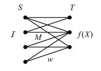
Figure 1: Independent assignment valuation

3.7 Concluding remarks of section 3

We collect here the conditions that characterize M^♮-concave set functions:

– Exchange property (M^♮-EXC) (Section 3.1)

– Multiple exchange property (M^♮-EXC_m)
    = Strong no complementarities property (SNC) (Section 3.1)

– Local exchange property (Theorems 3.2 and 3.3) (Section 3.1)

– Single improvement property (SI) (Section 3.2)

– Exchange property (B^♮-EXC) for the maximizers $D(p;f)$ (Section 3.3)

– Multiple (one-sided) exchange property for the maximizers $D(p;f)$
    = No complementarities property (NC) (Section 3.3)

– Multiple exchange property (NCsim) for the maximizers $D(p;f)$ (Section 3.3)

– Gross substitutability (GS) (Section 3.3)

– Parametrized substitutability (SC${}^{1}_{\rm{G}}$) (Section 3.4)

– Parametrized substitutability (SC${}^{2}_{\rm{G}}$) (Section 3.4)

4 M^♮-concave Function on $\mathbb{Z}^{n}$

In Section 3 we have considered M^♮-concave set functions, which correspond to single-unit valuations with substitutability. In this section we deal with M^♮-concave functions defined on integer vectors, $f:\mathbb{Z}^{n}\to\mathbb{R}\cup\{-\infty\}$, which correspond to multi-unit valuations with substitutability.

4.1 Exchange property

Let $N$ be a finite set, say, $N=\{1,2,\ldots,n\}$ for $n\geq 1$. For a vector $z\in\mathbb{R}^{N}$ in general, define the positive and negative supports of $z$ as

$${\rm supp}^{+}(z)=\{i\mid z_{i}>0\},\qquad{\rm supp}^{-}(z)=\{j\mid z_{j}<0\}.$$ (4.1)

Recall that, for $i\in N$, the $i$th unit vector is denoted by $\chi_{i}$.

We say that a function $f:\mathbb{Z}^{N}\to\mathbb{R}\cup\{-\infty\}$ with ${\rm dom\,}f\not=\emptyset$ is M^♮-concave, if, for any $x,y\in\mathbb{Z}^{N}$ and $i\in{\rm supp}^{+}(x-y)$, we have (i)

$$f(x)+f(y)\leq f(x-\chi_{i})+f(y+\chi_{i})$$ (4.2)

or (ii) there exists some $j\in{\rm supp}^{-}(x-y)$ such that

$$f(x)+f(y)\leq f(x-\chi_{i}+\chi_{j})+f(y+\chi_{i}-\chi_{j}).$$ (4.3)

This property is referred to as the exchange property. See Fig. 2, in which $(x^{\prime},y^{\prime})=(x-\chi_{i},y+\chi_{i})$ and $(x^{\prime\prime},y^{\prime\prime})=(x-\chi_{i}+\chi_{j},y+\chi_{i}-\chi_{j})$.

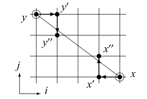
Figure 2: Nearer pair in the definition of M^♮-concave functions

A more compact expression of the exchange property is as follows:

(M^♮-EXC[$\mathbb{Z}$])

For any $x,y\in\mathbb{Z}^{N}$ and $i\in{\rm supp}^{+}(x-y)$, we have

$$f(x)+f(y)\leq\max_{j\in{\rm supp}^{-}(x-y)\cup\{0\}}\{f(x-\chi_{i}+\chi_{j})+f(y+\chi_{i}-\chi_{j})\},$$ (4.4)

where $\chi_{0}={\bf 0}$ (zero vector). In the above statement we may change “For any $x,y\in\mathbb{Z}^{N}$ ” to “For any $x,y\in{\rm dom\,}f$ ” since if $x\not\in{\rm dom\,}f$ or $y\not\in{\rm dom\,}f$, (4.4) trivially holds with $f(x)+f(y)=-\infty$. An M^♮-concave function $f$ with ${\rm dom\,}f\subseteq\{0,1\}^{N}$ can be identified with an M^♮-concave set function introduced in Section 3.1. A function $f$ is called M^♮-convex if $-f$ is M^♮-concave.

It follows from (M^♮-EXC[$\mathbb{Z}$]) that the effective domain $B={\rm dom\,}f$ of an M^♮-concave function $f$ has the following exchange property:

(B^♮-EXC[$\mathbb{Z}$])

For any $x,y\in B$ and $i\in{\rm supp}^{+}(x-y)$, we have (i) $x-\chi_{i}\in B$, $y+\chi_{i}\in B$  or  
(ii) there exists some $j\in{\rm supp}^{-}(x-y)$ such that $x-\chi_{i}+\chi_{j}\in B$, $y+\chi_{i}-\chi_{j}\in B$.

A set $B\subseteq\mathbb{Z}^{N}$ having this property is called an M^♮-convex set (or integral generalized polymatroid, integral g-polymatroid). An M^♮-convex set contained in the unit cube $\{0,1\}^{N}$ can be identified with an M^♮-convex family of subsets (Section 3.1).

M^♮-concavity can be characterized by a local exchange property under the assumption that function $f$ is (effectively) defined on an M^♮-convex set (Murota 1996c, 2003; Murota and Shioura 1999). The conditions (4.5)–(4.9) below are “local” in the sense that they require the exchangeability of the form of (4.4) only for some $(x,y)$ with $\|x-y\|_{1}\leq 4$.

Theorem 4.1.

A function $f:\mathbb{Z}^{N}\to\mathbb{R}\cup\{-\infty\}$ is M^♮-concave if and only if ${\rm dom\,}f$ is an M^♮-convex set and the following conditions hold:

$$f(x+2\chi_{i})+f(x)\leq 2f(x+\chi_{i})\qquad(\forall x\in\mathbb{Z}^{N},\ \forall i\in N),$$ (4.5)

$$f(x+\chi_{i}+\chi_{j})+f(x)\leq f(x+\chi_{i})+f(x+\chi_{j})\qquad(\forall x\in\mathbb{Z}^{N},\ \forall i,j\in N,\ i\not=j),$$ (4.6)

$$f(x+2\chi_{i})+f(x+\chi_{k})\leq f(x+\chi_{i}+\chi_{k})+f(x+\chi_{i})\qquad(\forall x\in\mathbb{Z}^{N},\ \forall i,k\in N,\ i\not=k),$$ (4.7)

$$f(x+\chi_{i}+\chi_{j})+f(x+\chi_{k})\leq\max\left[f(x+\chi_{i}+\chi_{k})+f(x+\chi_{j}),f(x+\chi_{j}+\chi_{k})+f(x+\chi_{i})\right]$$

$$\hskip 216.81pt(\forall x\in\mathbb{Z}^{N},\ \forall i,j,k\,\mbox{\rm(distinct})\in N),$$ (4.8)

$$f(x+\chi_{i}+\chi_{j})+f(x+\chi_{k}+\chi_{l})$$

$$\leq\max\left[f(x+\chi_{i}+\chi_{k})+f(x+\chi_{j}+\chi_{l}),f(x+\chi_{j}+\chi_{k})+f(x+\chi_{i}+\chi_{l})\right]$$

$$\hskip 173.44534pt(\forall x\in\mathbb{Z}^{N},\ \forall i,j,k,l\in N\ \mbox{\rm with}\ \{i,j\}\cap\{k,l\}=\emptyset),$$ (4.9)

where in (4.9) we allow the possibility of $i=j$ or $k=l$.

When the effective domain ${\rm dom\,}f$ is an M^♮-convex set such that $\bm{0}\in{\rm dom\,}f\subseteq\mathbb{Z}_{+}^{N}$, the local exchange condition above takes a simpler form that does not involve (4.9) (Theorem 6.8 of Shioura and Tamura 2015). To cover the case of ${\rm dom\,}f=\mathbb{Z}^{N}$ we weaken the assumption on ${\rm dom\,}f$ to:

$$x,y\in{\rm dom\,}f\Longrightarrow x\wedge y\in{\rm dom\,}f.$$ (4.10)

Theorem 4.2.

Let $f:\mathbb{Z}^{N}\to\mathbb{R}\cup\{-\infty\}$ be a function such that ${\rm dom\,}f$ is an M^♮-convex set satisfying (4.10). Then $f$ is M^♮-concave if and only if (4.5), (4.6), (4.7) and (4.8) hold.

Proof.

The proof of Theorem 6.8 of Shioura and Tamura (2015) works under the weaker condition (4.10). ∎

The local exchange property above admits a natural reformulation in terms of the discrete Hessian matrix when ${\rm dom\,}f=\mathbb{Z}^{N}$. For $x\in\mathbb{Z}^{N}$ and $i,j\in N$ define

$$H_{ij}(x)=f(x+\chi_{i}+\chi_{j})-f(x+\chi_{i})-f(x+\chi_{j})+f(x),$$ (4.11)

and let $H_{f}(x)=(H_{ij}(x)\mid i,j\in N)$ be the matrix consisting of those components. This matrix $H_{f}(x)$ is called the discrete Hessian matrix of $f$ at $x$. The following theorem, due to Hirai and Murota (2004) and Murota (2007), can be derived from Theorem 4.2.

Theorem 4.3.

A function $f:\mathbb{Z}^{N}\to\mathbb{R}$ is M^♮-concave if and only if the discrete Hessian matrix $H_{f}(x)=(H_{ij}(x))$ satisfies the following conditions for each $x\in\mathbb{Z}^{N}$:

$$H_{ij}(x)\leq 0 \mbox{for any $(i,j)$},$$ (4.12)

$$H_{ij}(x)\leq\max(H_{ik}(x),H_{jk}(x)) \mbox{if }\ \{i,j\}\cap\{k\}=\emptyset.$$ (4.13)

Proof.

The correspondence between the conditions in Theorems 4.2 and 4.3 is quite straightforward. With the use of (4.11) we can easily verify: (4.5) $\Leftrightarrow$ $H_{ii}(x)\leq 0$,  (4.6) $\Leftrightarrow$ $H_{ij}(x)\leq 0$ $(i\not=j)$,  (4.7) $\Leftrightarrow$ $H_{ii}(x)\leq H_{ik}(x)$ $(i\not=k)$,  and (4.8) $\Leftrightarrow$ $H_{ij}(x)\leq\max(H_{ik}(x),H_{jk}(x))$ ($i,j,k$: distinct). ∎

It is known (Theorem 6.19 of Murota 2003) that an M^♮-concave function $f:\mathbb{Z}^{N}\to\mathbb{R}\cup\{-\infty\}$ is submodular on the integer lattice, i.e.,

$$f(x)+f(y)\geq f(x\vee y)+f(x\wedge y)\qquad(x,y\in\mathbb{Z}^{N}).$$ (4.14)

More precisely, the condition (4.6) above is equivalent to the submodularity (4.14) as long as ${\rm dom\,}f$ is M^♮-convex (Proposition 6.1 of Shioura and Tamura 2015). Because of the additional conditions for M^♮-concavity, not every submodular function is M^♮-concave. Thus, M^♮-concave functions form a proper subclass of submodular functions on $\mathbb{Z}^{N}$.

It is also known (Theorem 4.6 of Murota 1996c, Theorem 6.42 of Murota 2003) that an M^♮-concave function $f:\mathbb{Z}^{N}\to\mathbb{R}\cup\{-\infty\}$ is concave-extensible, i.e., there exists a concave function $\overline{f}:\mathbb{R}^{N}\to\mathbb{R}\cup\{-\infty\}$ such that $\overline{f}(x)=f(x)$ for all $x\in\mathbb{Z}^{N}$.

Remark 4.1.

It follows from (M^♮-EXC[$\mathbb{Z}$]) that M^♮-concave functions enjoy the following exchange properties under size constraints (Lemmas 4.3 and 4.6 of Murota and Shioura 1999):
$\bullet$ For any $x,y\in\mathbb{Z}^{N}$ with $x(N)<y(N)$,

$$f(x)+f(y) \leq\max_{j\in{\rm supp}^{-}(x-y)}\{f(x+\chi_{j})+f(y-\chi_{j})\}.$$ (4.15)

$\bullet$ For any $x,y\in\mathbb{Z}^{N}$ with $x(N)=y(N)$ and $i\in{\rm supp}^{+}(x-y)$,

$$f(x)+f(y) \leq\max_{j\in{\rm supp}^{-}(x-y)}\{f(x-\chi_{i}+\chi_{j})+f(y+\chi_{i}-\chi_{j})\}.$$ (4.16)

The former property, in particular, implies the size-monotonicity of the induced choice function; see Theorem 4.9 and its proof.  

Remark 4.2.

If $B\subseteq\mathbb{Z}^{N}$ lies in a hyperplane with a constant component sum (i.e., $x(N)=y(N)$ for all $x,y\in B$), the exchange property (B^♮-EXC[$\mathbb{Z}$]) takes a simpler form (without the possibility of $j=0$): For any $x,y\in B$ and $i\in{\rm supp}^{+}(x-y)$, there exists some $j\in{\rm supp}^{-}(x-y)$ such that $x-\chi_{i}+\chi_{j}\in B$, $y+\chi_{i}-\chi_{j}\in B$. A set $B\subseteq\mathbb{Z}^{N}$ having this exchange property is called an M-convex set (or integral base polyhedron). An M^♮-concave function defined on an M-convex set is called an M-concave function (Murota 1996c, 2003). The exchange property for M-concavity reads: A function $f:\mathbb{Z}^{N}\to\mathbb{R}\cup\{-\infty\}$ is M-concave if and only if, for any $x,y\in\mathbb{Z}^{N}$ and $i\in{\rm supp}^{+}(x-y)$, it holds that

$$f(x)+f(y)\leq\max_{j\in{\rm supp}^{-}(x-y)}\{f(x-\chi_{i}+\chi_{j})+f(y+\chi_{i}-\chi_{j})\}.$$ (4.17)

M-concave functions and M^♮-concave functions are equivalent concepts, in that M^♮-concave functions in $n$ variables can be obtained as projections of M-concave functions in $n+1$ variables. More formally, let “$0$” denote a new element not in $N$ and $\tilde{N}=\{0\}\cup N$. A function $f:\mathbb{Z}^{N}\to\mathbb{R}\cup\{-\infty\}$ is M^♮-concave if and only if the function $\tilde{f}:\mathbb{Z}^{\tilde{N}}\to\mathbb{R}\cup\{-\infty\}$ defined by

$$\tilde{f}(x_{0},x)=\left\{\begin{array}[]{ll}f(x)&\mbox{ if $x_{0}={-}x(N)$}\\ -\infty&\mbox{ otherwise}\end{array}\right.\qquad(x_{0}\in\mathbb{Z},x\in\mathbb{Z}^{N})$$ (4.18)

is an M-concave function. A function $f$ is called M-convex if $-f$ is M-concave.  

4.2 Maximization and single improvement property

For an M^♮-concave function, the maximality of a function value is characterized by a local condition as follows, where $\chi_{0}={\bf 0}$ (Proposition 6.23 and Theorem 6.26 of Murota 2003).

Theorem 4.4.

Let $f:\mathbb{Z}^{N}\to\mathbb{R}\cup\{-\infty\}$ be an M^♮-concave function and $x\in{\rm dom\,}f$.

(1) If $f(x)<f(y)$ for $y\in{\rm dom\,}f$, then $f(x)<f(x-\chi_{i}+\chi_{j})$ for some $i\in{\rm supp}^{+}(x-y)\cup\{0\}$ and $j\in{\rm supp}^{-}(x-y)\cup\{0\}$.

(2) $x$ is a maximizer of $f$ if and only if

$$f(x) \geq f(x-\chi_{i}+\chi_{j})\quad(\forall\,i,j\in N\cup\{0\}).$$ (4.19)

For a vector $p=(p_{i}\mid i\in N)\in\mathbb{R}^{N}$ we use the notation $f[-p]$ to mean the function $f(x)-p^{\top}x$, where $p^{\top}$ means the transpose of $p$. That is,

$$f[-p](x)=f(x)-p^{\top}x\qquad(x\in\mathbb{Z}^{N}).$$ (4.20)

By considering the properties of (1) and (2) in Theorem 4.4 for $f[-p]$ with varying $p$, we are naturally led to (SSI[$\mathbb{Z}$]) and (SI[$\mathbb{Z}$]) below:

(SSI[$\mathbb{Z}$])

For any $p\in\mathbb{R}^{N}$ and $x,y\in{\rm dom\,}f$ with $f[-p](x)<f[-p](y)$, there exists $i\in{\rm supp}^{+}(x-y)\cup\{0\}$ and $j\in{\rm supp}^{-}(x-y)\cup\{0\}$ such that $f[-p](x)<f[-p](x-\chi_{i}+\chi_{j})$.

(SI[$\mathbb{Z}$])

For any $p\in\mathbb{R}^{N}$, if $x\in{\rm dom\,}f$ is not a maximizer of $f[-p]$, there exists $i\in N\cup\{0\}$ and $j\in N\cup\{0\}$ such that $f[-p](x)<f[-p](x-\chi_{i}+\chi_{j})$.

The stronger version (SSI[$\mathbb{Z}$]) is shown to be equivalent to M^♮-concavity (Theorem 7 of Murota and Tamura 2003a). This property is named the strong single improvement property in Shioura and Tamura (2015). The latter (SI[$\mathbb{Z}$]) is the vector version of single improvement property (Section 3.2), called the multi-unit single improvement property by Milgrom and Strulovici (2009). We can see from Theorem 13 of Milgrom and Strulovici (2009) that (SI[$\mathbb{Z}$]) is equivalent to M^♮-concavity under the assumption of concave-extensibility of $f$ and boundedness of ${\rm dom\,}f$.

4.3 Maximizers and gross substitutability

For a vector $p=(p_{i}\mid i\in N)\in\mathbb{R}^{N}$ we consider the maximizers of the function $f[-p](x)=f(x)-p^{\top}x$. We denote the set of these maximizers by

$$D(p;f)=\arg\max_{x}\{f(x)-p^{\top}x\}.$$ (4.21)

In economic applications, $p$ is a price vector and $D(p)=D(p;f)$ represents the demand correspondence.

It is one of the most fundamental facts in discrete convex analysis that the M^♮-concavity of a function is characterized in terms of the M^♮-convexity of its maximizers (Murota 1996c; Theorem 6.30 of Murota 2003; Murota and Shioura 1999).

Theorem 4.5.

Let $f:\mathbb{Z}^{N}\to\mathbb{R}\cup\{-\infty\}$ be a function with a bounded effective domain. Then $f$ is M^♮-concave if and only if, for every vector $p\in\mathbb{R}^{N}$, $D(p;f)$ is an M^♮-convex set. That is, $f$ satisfies (M^♮-EXC[$\mathbb{Z}$]) if and only if, for every $p\in\mathbb{R}^{N}$, $D(p;f)$ satisfies (B^♮-EXC[$\mathbb{Z}$]).

As a straightforward extension of the gross substitutes condition from single-unit valuations (Section 3.3) to multi-unit valuations it seems natural to conceive the following condition:

(GS[$\mathbb{Z}$])

For any $p,q\in\mathbb{R}^{N}$ with $p\leq q$ and $x\in D(p;f)$, there exists $y\in D(q;f)$ such that $x_{i}\leq y_{i}$ for all $i\in N$ with $p_{i}=q_{i}$.

It turns out, however, that this condition alone is too weak to be fruitful, mathematically and economically. Subsequently, several different strengthened forms of (GS[$\mathbb{Z}$]) are proposed in the literature (Danilov et al. 2003, Murota and Tamura 2003a, Milgrom and Strulovici 2009, Shioura and Tamura 2015).

Among others we start with the projected gross substitutes condition (PRJ-GS[$\mathbb{Z}$]) of Murota and Tamura (2003a):

(PRJ-GS[$\mathbb{Z}$])

For any $p,q\in\mathbb{R}^{N}$ with $p\leq q$, any $p_{0},q_{0}\in\mathbb{R}$ with $p_{0}\leq q_{0}$ and $x\in D(p-p_{0}\bm{1};f)$, there exists $y\in D(q-q_{0}\bm{1};f)$ such that (i) $x_{i}\leq y_{i}$ for all $i\in N$ with $p_{i}=q_{i}$ and (ii) $x(N)\geq y(N)$ if $p_{0}=q_{0}$,

where $x(N)=\sum_{i\in N}x_{i}$ and $y(N)=\sum_{i\in N}y_{i}$. By fixing $p_{0}=q_{0}=0$ in (PRJ-GS[$\mathbb{Z}$]) we obtain the following condition:

(GS&LAD[$\mathbb{Z}$])

For any $p,q\in\mathbb{R}^{N}$ with $p\leq q$ and $x\in D(p;f)$, there exists $y\in D(q;f)$ such that (i) $x_{i}\leq y_{i}$ for all $i\in N$ with $p_{i}=q_{i}$ and (ii) $x(N)\geq y(N)$.

As the acronym (GS&LAD[$\mathbb{Z}$]) shows, this condition is a combination of (GS[$\mathbb{Z}$]) above and the law of aggregate demand:

(LAD[$\mathbb{Z}$])

For any $p,q\in\mathbb{R}^{N}$ with $p\leq q$ and $x\in D(p;f)$, there exists $y\in D(q;f)$ such that $x(N)\geq y(N)$

considered by Hatfield and Milgrom (2005) and Milgrom and Strulovici (2009). Note, however, that imposing (GS&LAD[$\mathbb{Z}$]) on $f$ is not the same as imposing (GS[$\mathbb{Z}$]) and (LAD[$\mathbb{Z}$]) on $f$, since in (GS&LAD[$\mathbb{Z}$]) both (i) and (ii) must be satisfied by the same vector $y$. Obviously, (GS&LAD[$\mathbb{Z}$]) implies (GS[$\mathbb{Z}$]) and (LAD[$\mathbb{Z}$]). The amalgamated form (GS&LAD[$\mathbb{Z}$]) is given in Murota et al. (2013a), whereas the juxtaposition of (GS[$\mathbb{Z}$]) and (LAD[$\mathbb{Z}$]) is in Theorem 13 (iv) of Milgrom and Strulovici (2009). We may also consider the following variant (Shioura and Tamura 2015, Shioura and Yang 2015) of (GS&LAD[$\mathbb{Z}$]), where the vector $q$ takes a special form $p+\delta\chi_{k}$ with $k\in N$ and $\delta>0$:

(GS&LAD^′[$\mathbb{Z}$])

For any $p\in\mathbb{R}^{N}$, $k\in N$, $\delta>0$ and $x\in D(p;f)$, there exists $y\in D(p+\delta\chi_{k};f)$ such that (i) $x_{i}\leq y_{i}$ for all $i\in N\setminus\{k\}$ and (ii) $x(N)\geq y(N)$.

M^♮-concavity can be characterized by these properties as follows (Murota and Tamura 2003a, Danilov et al. 2003, Theorem 13 of Milgrom and Strulovici 2009, Theorem 4.1 of Shioura and Tamura 2015; Theorems 6.34 and 6.36 of Murota 2003). The theorem refers to two other conditions (SWGS[$\mathbb{Z}$]) and (SS[$\mathbb{Z}$]), which are explained in Remark 4.3 below.

Theorem 4.6.

Let $f:\mathbb{Z}^{N}\to\mathbb{R}\cup\{-\infty\}$ be a concave-extensible function with a bounded effective domain. Then we have the following equivalence: (M^♮-EXC[$\mathbb{Z}$]) $\iff$ (PRJ-GS[$\mathbb{Z}$]) $\iff$ (GS&LAD[$\mathbb{Z}$]) $\iff$ (GS[$\mathbb{Z}$]) & (LAD[$\mathbb{Z}$]) $\iff$ (GS&LAD^′[$\mathbb{Z}$]) $\iff$ (SWGS[$\mathbb{Z}$]). If ${\rm dom\,}f$ is contained in $\mathbb{Z}_{+}^{N}$, each of these conditions is equivalent to (SS[$\mathbb{Z}$]).

Remark 4.3.

The step-wise gross substitutes condition (Danilov et al. 2003) means:

(SWGS[$\mathbb{Z}$])

For any $p\in\mathbb{R}^{N}$, $k\in N$ and $x\in D(p;f)$, at least one of (i) and (ii) holds true:
(i) $x\in D(p+\delta\chi_{k};f)$ for all $\delta\geq 0$,
(ii) there exists $\delta\geq 0$ and $y\in D(p+\delta\chi_{k};f)$ such that $y_{k}=x_{k}-1$ and $y_{i}\geq x_{i}$ for all $i\in N\setminus\{k\}$.

The strong substitute condition (Milgrom and Strulovici 2009) for a multi-unit valuation $f$ means the condition (GS[$\mathbb{Z}$]) for the single-unit valuation $f^{\rm B}$ corresponding to $f$:

(SS[$\mathbb{Z}$])

The function $f^{\rm B}$ associated with $f$ satisfies the condition (GS[$\mathbb{Z}$]).

More specifically, the function $f^{\rm B}$ is defined as follows. Let $u\in\mathbb{Z}_{+}^{N}$ be a vector such that ${\rm dom\,}f\subseteq[\bm{0},u]_{\mathbb{Z}}$. Consider a set $N^{\rm B}=\{(i,\beta)\mid i\in N,\ \beta\in\mathbb{Z},\ 1\leq\beta\leq u_{i}\}$ and define $f^{\rm B}:\mathbb{Z}^{N^{\rm B}}\to\mathbb{R}\cup\{-\infty\}$ with ${\rm dom\,}f^{\rm B}\subseteq\{0,1\}^{N^{\rm B}}$ by

$${f}^{\rm B}({x}^{\rm B})=f(x),\quad x^{\rm B}\in\{0,1\}^{N^{\rm B}},\quad x_{i}=\sum_{\beta=1}^{u_{i}}x^{\rm B}_{(i,\beta)}\quad(i\in N).$$ (4.22)

 

4.4 Choice function

Let $b\in\mathbb{Z}_{+}^{N}$ be an upper bound vector and $\mathcal{B}=\{x\in\mathbb{Z}_{+}^{N}\mid x\leq b\}$ be the set of feasible vectors. A function $C:\mathcal{B}\to\mathcal{B}$ is called a choice function if $C(x)\leq x$ for all $x\in\mathcal{B}$. Three important properties are identified in the literature (Alkan and Gale 2003):

• $C$ is called consistent if  $C(x)\leq y\leq x$ implies $C(y)=C(x)$,

• $C$ is called persistent if  $x\geq y$ implies $y\wedge C(x)\leq C(y)$,

• $C$ is called size-monotone if  $x\geq y$ implies $|C(x)|\geq|C(y)|$, where $\displaystyle|C(x)|=\sum_{i\in N}C(x)_{i}$.

Remark 4.4.

Alkan and Gale (2003) considered the stable allocation model that extends the stable matching model of Alkan (2002). If the choice functions are consistent and persistent, the set of stable allocations is nonempty and forms a lattice. Moreover, if the choice functions are also size-monotone, the lattice of stable allocations is distributive and has several significant properties, called polarity, complementarity, and uni-size property.  

For a given function $f:\mathbb{Z}^{N}\to\mathbb{R}\cup\{-\infty\}$ we define

$$C(z)=C(z;f)=\arg\max\{f(y)\mid y\leq z\}.$$ (4.23)

In general, the maximizer may not be unique, and hence $C(z;f)\subseteq\mathbb{Z}^{N}$. We also have the possibility of $C(z;f)=\emptyset$ to express the nonexistence of a maximizer.

An important property of M^♮-concave functions, closely related to persistence, is found in Lemma 1 of Eguchi et al. (2003); see also Lemma 5.2 of Fujishige and Tamura (2006).

Theorem 4.7.

Let $f:\mathbb{Z}^{N}\rightarrow\mathbb{R}\cup\{-\infty\}$ be an M^♮-concave function. Then the following hold.

(SC¹[$\mathbb{Z}$])

For any $z_{1},z_{2}\in\mathbb{Z}^{N}$ with $z_{1}\geq z_{2}$ and $C(z_{2};f)\neq\emptyset$ and for any $x_{1}\in C(z_{1};f)$, there exists $x_{2}\in C(z_{2};f)$ such that $z_{2}\wedge x_{1}\leq x_{2}$.

(SC²[$\mathbb{Z}$])

For any $z_{1},z_{2}\in\mathbb{Z}^{N}$ with $z_{1}\geq z_{2}$ and $C(z_{1};f)\neq\emptyset$ and for any $x_{2}\in C(z_{2};f)$, there exists $x_{1}\in C(z_{1};f)$ such that $z_{2}\wedge x_{1}\leq x_{2}$.

Proof.

Assume $z_{1}\geq z_{2}$. For $x_{1}\leq z_{1}$ and $x_{2}\leq z_{2}$ define

$$\varPhi(x_{1},x_{2})=\sum\{(x_{1})_{i}-(x_{2})_{i}\mid i\in{\rm supp}^{+}((z_{2}\wedge x_{1})-x_{2})\}.$$

Proof of (SC¹[$\mathbb{Z}$]): Let $x_{1}\in C(z_{1};f)$ and take $x_{2}\in C(z_{2};f)$ with minimum $\varPhi(x_{1},x_{2})$. To prove by contradiction, suppose that there exists $i\in{\rm supp}^{+}((z_{2}\wedge x_{1})-x_{2})$. Since $i\in{\rm supp}^{+}(x_{1}-x_{2})$, (M^♮-EXC[$\mathbb{Z}$]) implies there exists $j\in{\rm supp}^{-}(x_{1}-x_{2})\cup\{0\}$ such that

$$f(x_{1})+f(x_{2})\leq f(x_{1}-\chi_{i}+\chi_{j})+f(x_{2}+\chi_{i}-\chi_{j}).$$

Here we have $x_{1}-\chi_{i}+\chi_{j}\leq z_{1}$ and $x_{2}+\chi_{i}-\chi_{j}\leq z_{2}$; the former is obvious if $j=0$ and otherwise, it follows from $(x_{1})_{j}<(x_{2})_{j}\leq(z_{2})_{j}\leq(z_{1})_{j}$, and the latter follows from $(x_{2})_{i}<(z_{2})_{i}$. This implies that $f(x_{1}-\chi_{i}+\chi_{j})\leq f(x_{1})$ and $f(x_{2}+\chi_{i}-\chi_{j})\leq f(x_{2})$ since $x_{1}\in C(z_{1};f)$ and $x_{2}\in C(z_{2};f)$. Therefore, the inequalities are in fact equalities, and $x_{1}-\chi_{i}+\chi_{j}\in C(z_{1};f)$ and $x_{2}+\chi_{i}-\chi_{j}\in C(z_{2};f)$. But we have $\varPhi(x_{1},x_{2}+\chi_{i}-\chi_{j})=\varPhi(x_{1},x_{2})-1$, which contradicts the choice of $x_{2}$.

Proof of (SC²[$\mathbb{Z}$]): Let $x_{2}\in C(z_{2};f)$ and take $x_{1}\in C(z_{1};f)$ with minimum $\varPhi(x_{1},x_{2})$. By the same argument as above we obtain $x_{1}-\chi_{i}+\chi_{j}\in C(z_{1};f)$ with $\varPhi(x_{1}-\chi_{i}+\chi_{j},x_{2})=\varPhi(x_{1},x_{2})-1$. This is a contradiction to the choice of $x_{1}$. ∎

When the maximizer is unique in (4.23) for every $z$, we say that $f$ is unique-selecting. In the following we assume that $f$ is unique-selecting and

$$\bm{0}\in{\rm dom\,}f\subseteq\mathbb{Z}_{+}^{N}.$$ (4.24)

Then $C$ in (4.23) can be regarded as a choice function $C:\mathcal{B}\to\mathcal{B}$.

The induced choice function $C$ is obviously consistent for any valuation function $f$. For persistence, M^♮-concavity plays an essential role. The following theorem of Eguchi et al. (2003) can be obtained as a corollary of Theorem 4.7, since for unique-selecting valuation functions, (SC¹[$\mathbb{Z}$]) and (SC²[$\mathbb{Z}$]) are equivalent and both coincide with persistence.

Theorem 4.8.

Every unique-selecting M^♮-concave function $f:\mathbb{Z}^{N}\to\mathbb{R}\cup\{-\infty\}$ with (4.24) induces a persistent choice function.

The size-monotonicity is also implied by M^♮-concavity (Murota and Yokoi 2015).

Theorem 4.9.

Every unique-selecting M^♮-concave function $f:\mathbb{Z}^{N}\to\mathbb{R}\cup\{-\infty\}$ with (4.24) induces a size-monotone choice function.

Proof.

The proof is based on the exchange property (4.15) in Remark 4.1. To prove by contradiction, suppose that there exist $x,y\in\mathbb{Z}^{N}$ such that $x\geq y$ and $|C(x;f)|<|C(y;f)|$. Set $x^{*}=C(x;f)$ and $y^{*}=C(y;f)$. Then $|x^{*}|<|y^{*}|$. By the exchange property (4.15) there exists $j\in{\rm supp}^{-}(x^{*}-y^{*})$ such that $f(x^{*})+f(y^{*})\leq f(x^{*}+\chi_{j})+f(y^{*}-\chi_{j})$. Here we have $f(x^{*}+\chi_{j})<f(x^{*})$ since $x^{*}+\chi_{j}\leq x$ by $x^{*}_{j}<y^{*}_{j}\leq y_{j}\leq x_{j}$ and $x^{*}$ is the unique maximizer. We also have $f(y^{*}-\chi_{j})<f(y^{*})$ since $y^{*}-\chi_{j}\leq y^{*}\leq y$ and $y^{*}$ is the unique maximizer. This is a contradiction. ∎

Thus, M^♮-concave valuation functions entail the three desired properties, consistency, persistence, and size-monotonicity. Recall Remark 4.4 for the implications of this fact.

Theorem 4.10.

For a unique-selecting M^♮-concave value function $f:\mathbb{Z}^{N}\to\mathbb{R}\cup\{-\infty\}$ with (4.24), the choice function $C$ induced from $f$ is consistent, persistent, and size-monotone.

Finally, we mention a theorem that characterizes M^♮-concavity in terms of a parametrized version of (SC¹[$\mathbb{Z}$]) and (SC²[$\mathbb{Z}$]). Recall from (4.20) the notation $f[-p](x)=f(x)-p^{\top}x$ for $p\in\mathbb{R}^{N}$ and $x\in\mathbb{Z}^{N}$. If $f$ is an M^♮-concave function (not assumed to be unique-selecting), $f[-p]$ is also M^♮-concave, and hence is equipped with the properties (SC¹[$\mathbb{Z}$]) and (SC²[$\mathbb{Z}$]) by Theorem 4.7. In other words, an M^♮-concave function $f$ has the following properties.

(SC${}^{1}_{\rm\bf{G}}$[$\mathbb{Z}$])

For any $p\in\mathbb{R}^{N}$, $f[-p]$ satisfies (SC¹[$\mathbb{Z}$]).

(SC${}^{2}_{\rm\bf{G}}$[$\mathbb{Z}$])

For any $p\in\mathbb{R}^{N}$, $f[-p]$ satisfies (SC²[$\mathbb{Z}$]).

The following theorem, due to Farooq and Shioura (2005), states that each of these conditions characterizes M^♮-concavity.

Theorem 4.11.

For a function $f:\mathbb{Z}^{N}\to\mathbb{R}\cup\{-\infty\}$ with a bounded nonempty effective domain, we have the equivalence: $f$ is M^♮-concave $\iff$ (SC${}^{1}_{\rm{G}}$[$\mathbb{Z}$]) $\iff$ (SC${}^{2}_{\rm{G}}$[$\mathbb{Z}$]).

4.5 Twisted M^♮-concavity

Let $W$ be a subset of $N$. For any vector $x\in\mathbb{Z}^{N}$ we define $\mathrm{tw}(x)\in\mathbb{Z}^{N}$ by specifying its $i$th component $\mathrm{tw}(x)_{i}$ as

$$\mathrm{tw}(x)_{i}=\left\{\begin{array}[]{ll}\phantom{-}x_{i}&(i\in N\setminus W),\\ -x_{i}&(i\in W).\\ \end{array}\right.$$ (4.25)

A function $f:\mathbb{Z}^{N}\to\mathbb{R}\cup\{-\infty\}$ is said to be a twisted M^♮-concave function with respect to $W$, if the function $\tilde{f}:\mathbb{Z}^{N}\to\mathbb{R}\cup\{-\infty\}$ defined by

$$\tilde{f}(x)=f(\mathrm{tw}(x))\qquad(x\in\mathbb{Z}^{N})$$ (4.26)

is an M^♮-concave function (Ikebe and Tamura 2015). The same concept has been introduced by Shioura and Yang (2015), almost at the same time and independently, under the name of GM-concave functions. Note that $f$ is twisted M^♮-concave with respect to $W$ if and only if it is twisted M^♮-concave with respect to $U=N\setminus W$.

Mathematically, twisted M^♮-concavity is equivalent to the original M^♮-concavity through twisting, and all the properties and theorems about M^♮-concave functions can be translated into those about twisted M^♮-concave functions. In such translations it is often adequate to define the twisted demand correspondence as

$$\tilde{D}(p;f)=\arg\max_{x}\{f(x)-\mathrm{tw}(p)^{\top}x\}.$$ (4.27)

A twisted version of (GS&LAD^′[$\mathbb{Z}$]) is introduced by Ikebe et al. (2015) as the generalized full substitutes (GFS[$\mathbb{Z}$]) condition:

(GFS[$\mathbb{Z}$])

(i) For any $p\in\mathbb{R}^{N}$, $\tilde{D}(p;f)$ is a discrete convex set.
(ii) For any $p\in\mathbb{R}^{N}$, $k\in U$, $\delta>0$, and $x\in\tilde{D}(p;f)$, there exists $y\in\tilde{D}(p+\delta\chi_{k};f)$ such that

$$x_{i}\leq y_{i}\ \ (\forall i\in U\setminus\{k\}),\quad x_{i}\geq y_{i}\ \ (\forall i\in W),\quad x(U)-x(W)\geq y(U)-y(W).$$ (4.28)

(iii) For any $p\in\mathbb{R}^{N}$, $k\in W$, $\delta>0$, and $x\in\tilde{D}(p;f)$, there exists $y\in\tilde{D}(p-\delta\chi_{k};f)$ such that

$$x_{i}\leq y_{i}\ \ (\forall i\in W\setminus\{k\}),\quad x_{i}\geq y_{i}\ \ (\forall i\in U),\quad x(W)-x(U)\geq y(W)-y(U).$$ (4.29)

The following theorem (Ikebe et al. 2015) characterizes twisted M^♮-concavity in terms of this condition.

Theorem 4.12.

Let $f:\mathbb{Z}^{N}\to\mathbb{R}\cup\{-\infty\}$ be a concave-extensible function with a bounded effective domain. Then $f$ satisfies (GFS[$\mathbb{Z}$]) if and only if it is a twisted M^♮-concave function with respect to $W$.

In the modeling of a trading network (supply chain network), where an agent is identified with a vertex (node) of the network, each vertex (agent) is associated with a valuation function $f$ defined on the set of arcs incident to the vertex. Denoting the set of in-coming arcs to the vertex by $U$ and the set of out-going arcs from the vertex by $W$, the function $f$ is defined on $U\cup W$. Twisted M^♮-concave functions are used effectively in this context (Ikebe and Tamura 2015, Ikebe et al. 2015, Candogan et al. 2016). See Section 14.2.

With the use of the ordinary (un-twisted) demand correspondence

$$D(p;f)=\arg\max_{x}\{f(x)-p^{\top}x\},$$ (4.30)

a similar condition was formulated by Shioura and Yang (2015), independently of Ikebe et al. (2015), to deal with economies with two classes of indivisible goods such that goods in the same class are substitutable and goods across two classes are complementary. The condition, called the generalized gross substitutes and complements (GGSC[$\mathbb{Z}$]) condition, reads as follows:

(GGSC[$\mathbb{Z}$])

(i) For any $p\in\mathbb{R}^{N}$, $D(p;f)$ is a discrete convex set.
(ii) For any $p\in\mathbb{R}^{N}$, $k\in U$, $\delta>0$, and $x\in D(p;f)$, there exists $y\in D(p+\delta\chi_{k};f)$ that satisfies (4.28).
(iii) For any $p\in\mathbb{R}^{N}$, $k\in W$, $\delta>0$, and $x\in D(p;f)$, there exists $y\in D(p+\delta\chi_{k};f)$ that satisfies (4.29).

This condition also characterizes twisted M^♮-concavity (Shioura and Yang 2015).

Theorem 4.13.

Let $f:\mathbb{Z}^{N}\to\mathbb{R}\cup\{-\infty\}$ be a concave-extensible function with a bounded effective domain. Then $f$ satisfies (GGSC[$\mathbb{Z}$]) if and only if it is a twisted M^♮-concave function with respect to $W$.

Although Theorems 4.12 and 4.13 have significances in different contexts, they are in fact two variants of the same mathematical statement. Note that (GSF[$\mathbb{Z}$]) and (GGSC[$\mathbb{Z}$]) are equivalent, since

$$D(p;f)=\tilde{D}(\mathrm{tw}(p);f),\qquad\mathrm{tw}(p+\delta\chi_{k})=\left\{\begin{array}[]{ll}\mathrm{tw}(p)+\delta\chi_{k}&(k\in U),\\ \mathrm{tw}(p)-\delta\chi_{k}&(k\in W).\\ \end{array}\right.$$

The multi-unit (or vector) version of the same-side substitutability (SSS) and the cross-side complementarity (CSC) of Ostrovsky (2008) can be formulated for a correspondence $C:\mathbb{Z}^{N}\to 2^{\mathbb{Z}^{N}}$ as follows, where, for any $z\in\mathbb{Z}^{N}$, the subvector of $z$ on $U$ is denoted by $z^{U}\in\mathbb{Z}^{U}$ and similarly the subvector on $W$ by $z^{W}\in\mathbb{Z}^{W}$.

(SSS-CSC¹[$\mathbb{Z}$])

(i) For any $z_{1},z_{2}\in\mathbb{Z}^{N}$ with $z_{1}^{U}\geq z_{2}^{U}$, $z_{1}^{W}=z_{2}^{W}$ and $C(z_{2})\neq\emptyset$ and for any $x_{1}\in C(z_{1})$, there exists $x_{2}\in C(z_{2})$ such that $z_{2}^{U}\wedge x_{1}^{U}\leq x_{2}^{U}$ and $x_{1}^{W}\geq x_{2}^{W}$, and (ii) the same statement with $U$ and $W$ interchanged.

(SSS-CSC²[$\mathbb{Z}$])

(i) For any $z_{1},z_{2}\in\mathbb{Z}^{N}$ with $z_{1}^{U}\geq z_{2}^{U}$, $z_{1}^{W}=z_{2}^{W}$ and $C(z_{1})\neq\emptyset$ and for any $x_{2}\in C(z_{2})$ there exists $x_{1}\in C(z_{1})$, such that $z_{2}^{U}\wedge x_{1}^{U}\leq x_{2}^{U}$ and $x_{1}^{W}\geq x_{2}^{W}$, and (ii) the same statement with $U$ and $W$ interchanged.

The following theorem (Ikebe and Tamura 2015) states that these two properties are implied by twisted M^♮-concavity. Recall from (4.23) that a valuation function $f$ induces the correspondence $C(z)=C(z;f)=\arg\max\{f(y)\mid y\leq z\}$ $(z\in\mathbb{Z}^{N})$.

Theorem 4.14.

For any twisted M^♮-concave function $f:\mathbb{Z}^{N}\to\mathbb{R}\cup\{-\infty\}$, the induced correspondence $C$ has the properties (SSS-CSC¹[$\mathbb{Z}$]) and (SSS-CSC²[$\mathbb{Z}$]).

Proof.

We prove (SSS-CSC¹[$\mathbb{Z}$])-(i) and (SSS-CSC²[$\mathbb{Z}$])-(i); the proofs of (SSS-CSC¹[$\mathbb{Z}$])-(ii) and (SSS-CSC²[$\mathbb{Z}$])-(ii) are obtained by interchanging $U$ and $W$. Assume $z_{1}^{U}\geq z_{2}^{U}$, $z_{1}^{W}=z_{2}^{W}$ and $C(z_{1};f)\neq\emptyset$, and let $\tilde{f}$ be the M^♮-concave function in (4.26) associated with $f$. For $x_{1}\leq z_{1}$ and $x_{2}\leq z_{2}$ define

$$\varPhi(x_{1},x_{2})= \sum\{(x_{1})_{i}-(x_{2})_{i}\mid i\in U\cap{\rm supp}^{+}((z_{2}\wedge x_{1})-x_{2})\}$$

$$+\sum\{(x_{2})_{i}-(x_{1})_{i}\mid i\in W\cap{\rm supp}^{+}(x_{2}-x_{1})\}.$$

Proof of (SSS-CSC¹[$\mathbb{Z}$])-(i):  Let $x_{1}\in C(z_{1};f)$ and take $x_{2}\in C(z_{2};f)$ with $\varPhi(x_{1},x_{2})$ minimum. To prove by contradiction, suppose that there exists

$$i\in\big{(}U\cap{\rm supp}^{+}((z_{2}\wedge x_{1})-x_{2})\big{)}\cup\big{(}W\cap{\rm supp}^{+}(x_{2}-x_{1})\big{)}.$$

Then $i\in{\rm supp}^{+}(\mathrm{tw}(x_{1})-\mathrm{tw}(x_{2}))$, and (M^♮-EXC[$\mathbb{Z}$]) for $\tilde{f}$ implies that there exists $j\in{\rm supp}^{-}(\mathrm{tw}(x_{1})-\mathrm{tw}(x_{2}))\cup\{0\}$ such that

$$\tilde{f}(\mathrm{tw}(x_{1}))+\tilde{f}(\mathrm{tw}(x_{2}))\leq\tilde{f}(\mathrm{tw}(x_{1})-\chi_{i}+\chi_{j})+\tilde{f}(\mathrm{tw}(x_{2})+\chi_{i}-\chi_{j}).$$

Letting $\hat{x}_{1}=\mathrm{tw}(\mathrm{tw}(x_{1})-\chi_{i}+\chi_{j}))$ and $\hat{x}_{2}=\mathrm{tw}(\mathrm{tw}(x_{2})+\chi_{i}-\chi_{j}))$ we can express the above inequality as

$$f(x_{1})+f(x_{2})\leq f(\hat{x}_{1})+f(\hat{x}_{2}).$$

By considering all possibilities ($i\in U$ or $i\in W$, and $j\in U$ or $j\in W$ or $j=0$), we can verify that $\hat{x}_{1}\leq z_{1}$ and $\hat{x}_{2}\leq z_{2}$, from which follow $f(\hat{x}_{1})\leq f(x_{1})$ and $f(\hat{x}_{2})\leq f(x_{2})$ since $x_{1}\in C(z_{1};f)$ and $x_{2}\in C(z_{2};f)$. Therefore, the inequalities are in fact equalities, and $\hat{x}_{1}\in C(z_{1};f)$ and $\hat{x}_{2}\in C(z_{2};f)$. But we have $\varPhi(x_{1},\hat{x}_{2})=\varPhi(x_{1},x_{2})-1$, which contradicts the choice of $x_{2}$.

Proof of (SSS-CSC²[$\mathbb{Z}$])-(i):  Let $x_{2}\in C(z_{2};f)$ and take $x_{1}\in C(z_{1};f)$ with minimum $\varPhi(x_{1},x_{2})$. By the same argument as above we obtain $\hat{x}_{1}\in C(z_{1};f)$ with $\varPhi(\hat{x}_{1},x_{2})=\varPhi(x_{1},x_{2})-1$. This is a contradiction to the choice of $x_{1}$. ∎

4.6 Examples

Here are some examples of M^♮-concave functions in integer variables.

1. A linear (or affine) function

   $$f(x)=\alpha+\langle p,x\rangle$$ (4.31)

   with $p\in\mathbb{R}^{N}$ and $\alpha\in\mathbb{R}$ is M^♮-concave if ${\rm dom\,}f$ is an M^♮-convex set.

2. A quadratic function $f:\mathbb{Z}^{N}\to\mathbb{R}$ defined by

   $$f(x)=\sum_{i=1}^{n}\sum_{j=1}^{n}a_{ij}x_{i}x_{j}$$ (4.32)

   with $a_{ij}=a_{ji}\in\mathbb{R}$ $(i,j=1,\ldots,n)$ is M^♮-concave if and only if

   $$a_{ij}\leq 0\mbox{ \ for all $(i,j)$, \ \ and}\quad a_{ij}\leq\max(a_{ik},a_{jk})\ \mbox{ if }\ \{i,j\}\cap\{k\}=\emptyset.$$ (4.33)

   The Hessian matrix $H_{f}(x)=(H_{ij}(x))$ defined in (4.11) is given by $H_{ij}(x)=2a_{ij}$, and (4.33) above is consistent with (4.12), (4.13) in Theorem 4.3.

3. A function $f:\mathbb{Z}^{N}\to\mathbb{R}\cup\{-\infty\}$ is called separable concave if it can be represented as

   $$f(x)=\sum_{i\in N}\varphi_{i}(x_{i})\qquad(x\in\mathbb{Z}^{N})$$ (4.34)

   for univariate concave functions $\varphi_{i}:\mathbb{Z}\to\mathbb{R}\cup\{-\infty\}$ $(i\in N)$. A separable concave function is M^♮-concave. In (4.4) for (M^♮-EXC[$\mathbb{Z}$]) we can always take $j=0$, i.e., (4.2).

4. A function $f:\mathbb{Z}^{N}\to\mathbb{R}\cup\{-\infty\}$ is called laminar concave if it can be represented as

   $$f(x)=\sum_{A\in\mathcal{T}}\varphi_{A}(x(A))\qquad(x\in\mathbb{Z}^{N})$$ (4.35)

   for a laminar family $\mathcal{T}\subseteq 2^{N}$ and a family of univariate concave functions $\varphi_{A}:\mathbb{Z}\to\mathbb{R}\cup\{-\infty\}$ indexed by $A\in\mathcal{T}$, where $x(A)=\sum_{i\in A}x_{i}$. A laminar concave function is M^♮-concave; see Note 6.11 of Murota (2003) for a proof. A special case of (4.35) with $\mathcal{T}=\{\{1\},\{2\},\ldots,\{n\}\}$ reduces to the separable convex function (4.34).

5. M^♮-concave functions arise from the maximum weight of nonlinear network flows. Let $G=(V,A)$ be a directed graph with two disjoint vertex subsets $S\subseteq V$ and $T\subseteq V$ specified as the entrance and the exit. Suppose that, for each arc $a\in A$, we are given a univariate concave function $\varphi_{a}:\mathbb{Z}\to\mathbb{R}\cup\{-\infty\}$ representing the weight of flow on the arc $a$. Let $\xi\in\mathbb{Z}^{A}$ be a vector representing an integer flow, and $\partial\xi\in\mathbb{Z}^{V}$ be the boundary of flow $\xi$ defined by

   $$\begin{array}[]{l}\partial\xi(v)=\sum\{\xi(a)\mid\mbox{ arc $a$ leaves $v$ }\}-\sum\{\xi(a)\mid\mbox{ arc $a$ enters $v$ }\}\quad(v\in V).\end{array}$$ (4.36)

   Then, the maximum weight of a flow that realizes a supply/demand specification on the exit $T$ in terms of $x\in\mathbb{Z}^{T}$ is expressed by

   $$f(x)=\sup_{\xi}\big{\{}\sum_{a\in A}\varphi_{a}(\xi(a))\mid(\partial\xi)(v)=-x(v)\ (v\in T),\ (\partial\xi)(v)=0\ (v\in V\setminus(S\cup T))\big{\}},$$ (4.37)

   where no constraint is imposed on $(\partial\xi)(v)$ for entrance vertices $v\in S$. This function is M^♮-concave, provided that $f$ does not take the value $+\infty$ and ${\rm dom\,}f$ is nonempty. If $S=\emptyset$, the function $f$ is M-concave, since $\sum_{v\in T}x(v)=-\sum_{v\in T}(\partial\xi)(v)=\sum_{v\in V\setminus T}(\partial\xi)(v)=0$ in this case. See Example 2.3 of Murota (1998) and Section 2.2.2 of Murota (2003) for details. The maximum weight of a matching in (3.26) can be understood as a special case of (4.37).

4.7 Concluding remarks of section 4

The concept of M-convex functions is formulated by Murota (1996c) as a generalization of valuated matroids of Dress and Wenzel (1990, 1992). Then M^♮-convex functions are introduced by Murota and Shioura (1999) as a variant of M-convex functions. Quasi M-convex functions are introduced by Murota and Shioura (2003). The concept of M-convex functions is extended to functions on jump systems by Murota (2006); see also Kobayashi et al. (2007).

Unimodularity is closely related to discrete convexity. For a fixed unimodular matrix $U$ we may consider a change of variables $x\mapsto Ux$ for $x\in\mathbb{Z}^{n}$ to define a class of functions $\{f(Ux)\mid f:\mbox{M${}^{\natural}$-concave}\}$ as a variant of M^♮-concave functions. Twisted M^♮-concave functions (Section 4.5) are a typical example of this construction with $U={\rm diag}(1,\ldots,1,-1,\ldots,-1)$; see Sun and Yang (2008) and Section 14.5 for further discussion in this direction.

5 M^♮-concave Function on $\mathbb{R}^{n}$

In Sections 3 and 4, we have considered M^♮-concave functions on $2^{N}$ and $\mathbb{Z}^{N}$, which correspond to valuations for indivisible goods with substitutability. In this section we deal with M^♮-concave functions in real vectors, $f:\mathbb{R}^{N}\to\mathbb{R}\cup\{-\infty\}$, which correspond to valuations for divisible goods with substitutability. M^♮-concave functions in real variables are investigated by Murota and Shioura (2000, 2004a, 2004b).

5.1 Exchange property

We say that a function $f:\mathbb{R}^{N}\to\mathbb{R}\cup\{-\infty\}$ is M^♮-concave if it is a concave function (in the ordinary sense) that satisfies

(M^♮-EXC[$\mathbb{R}$])

For any $x,y\in\mathbb{R}^{N}$ and $i\in{\rm supp}^{+}(x-y)$, there exist $j\in{\rm supp}^{-}(x-y)\cup\{0\}$ and a positive number $\alpha_{0}\in\mathbb{R}_{++}$ such that

$$f(x)+f(y)\leq f(x-\alpha(\chi_{i}-\chi_{j}))+f(y+\alpha(\chi_{i}-\chi_{j}))$$ (5.1)

for all $\alpha\in\mathbb{R}$ with $0\leq\alpha\leq\alpha_{0}$.

In the following we restrict ourselves to closed proper M^♮-concave functions, for which the closure of the effective domain ${\rm dom\,}f$ is a well-behaved polyhedron (g-polymatroid, or M^♮-convex polyhedron); see Theorem 3.2 of Murota and Shioura (2008). Often we are interested in polyhedral M^♮-concave functions.

Remark 5.1.

It follows from (M^♮-EXC[$\mathbb{R}$]) that M^♮-concave functions enjoy the following exchange properties under size constraints:
$\bullet$ For any $x,y\in\mathbb{R}^{N}$ with $x(N)<y(N)$, there exists $\alpha_{0}\in\mathbb{R}_{++}$ such that

$$f(x)+f(y) \leq\max_{j\in{\rm supp}^{-}(x-y)}\{f(x+\alpha\chi_{j})+f(y-\alpha\chi_{j})\}$$ (5.2)

for all $\alpha\in\mathbb{R}$ with $0\leq\alpha\leq\alpha_{0}$.
$\bullet$ For any $x,y\in\mathbb{R}^{N}$ with $x(N)=y(N)$ and $i\in{\rm supp}^{+}(x-y)$, there exists $\alpha_{0}\in\mathbb{R}_{++}$ such that

$$f(x)+f(y) \leq\max_{j\in{\rm supp}^{-}(x-y)}\{f(x-\alpha(\chi_{i}-\chi_{j}))+f(y+\alpha(\chi_{i}-\chi_{j}))\}$$ (5.3)

for all $\alpha\in\mathbb{R}$ with $0\leq\alpha\leq\alpha_{0}$.  

Remark 5.2.

If ${\rm dom\,}f\subseteq\mathbb{R}^{N}$ lies in a hyperplane with a constant component sum (i.e., $x(N)=y(N)$ for all $x,y\in{\rm dom\,}f$), the exchange property (M^♮-EXC[$\mathbb{R}$]) takes a simpler form excluding the possibility of $j=0$. A function $f:\mathbb{R}^{N}\to\mathbb{R}\cup\{-\infty\}$ having this exchange property is called an M-concave function. That is, a concave function $f$ is M-concave if and only if (5.3) holds.  

5.2 Maximizers and gross substitutability

For $p\in\mathbb{R}^{N}$ we denote the set of the maximizers of $f[-p](x)=f(x)-p^{\top}x$ by $D(p;f)\subseteq\mathbb{R}^{N}$ (cf. (4.21)). M^♮-concavity of a function $f$ is characterized by the M^♮-convexity of $D(p;f)$ (Theorem 5.2 of Murota and Shioura 2000).

Theorem 5.1.

A polyhedral concave function $f:\mathbb{R}^{N}\to\mathbb{R}\cup\{-\infty\}$ is M^♮-concave if and only if, for every vector $p\in\mathbb{R}^{N}$, $D(p;f)$ is an M^♮-convex polyhedron.

(GS[$\mathbb{R}$])

For any $p,q\in\mathbb{R}^{N}$ with $p\leq q$ and $x\in D(p;f)$, there exists $y\in D(q;f)$ such that $x_{i}\leq y_{i}$ for all $i\in N$ with $p_{i}=q_{i}$.

The following theorem is given by Danilov et al. (2003).

Theorem 5.2.

A polyhedral M^♮-concave function $f:\mathbb{R}^{N}\to\mathbb{R}\cup\{-\infty\}$ with a bounded effective domain satisfies (GS[$\mathbb{R}$]).

Proof.

This follows from Theorem 7.5 (2) and Theorem 7.7 in Section 7.2. ∎

Example 5.1.

Here is an example to show that (GS[$\mathbb{R}$]) does not imply M^♮-concavity. Let $f:\mathbb{R}^{2}\to\mathbb{R}$ be defined by $f(x_{1},x_{2})=\min(2,x_{1}+2x_{2})$ on ${\rm dom\,}f=\mathbb{R}^{2}$. This function is not M^♮-concave because (M^♮-EXC[$\mathbb{R}$]) fails for $x=(2,0)$, $y=(0,1)$ and $i=1$. However, it satisfies (GS[$\mathbb{R}$]), which can be verified easily. Thus the converse of Theorem 5.2 does not hold.  

5.3 Choice function

In Theorem 4.10 in Section 4.4 we have seen, for the multi-unit indivisible goods, the choice function induced from a unique-selecting M^♮-concave value function is consistent, persistent, and size-monotone in the sense of Alkan and Gale (2003). In this section we point out that this is also the case with divisible goods; recall Remark 4.4 in Section 4.4 for the implications of this fact.

For a choice function $C:\mathcal{B}\to\mathcal{B}$ with $\mathcal{B}=\{x\in\mathbb{R}_{+}^{N}\mid x\leq b\}$ for some $b\in\mathbb{R}_{+}^{N}$, consistency means $[\ C(x)\leq y\leq x\Rightarrow C(y)=C(x)\ ]$, persistence means $[\ x\geq y\Rightarrow y\wedge C(x)\leq C(y)\ ]$, and size-monotonicity means $[\ x\geq y\Rightarrow|C(x)|\geq|C(y)|\ ]$, where $|C(x)|=\sum_{i\in N}C(x)_{i}$ (sum of the components).

Theorem 5.3.

For a unique-selecting M^♮-concave value function $f:\mathbb{R}^{N}\to\mathbb{R}\cup\{-\infty\}$ with $\bm{0}\in{\rm dom\,}f\subseteq\mathbb{R}_{+}^{N}$, the induced choice function $C(x;f)=\arg\max\{f(y)\mid y\leq x\}$ is consistent, persistent, and size-monotone.

Proof.

The consistency is obvious from the definition of $C(x;f)$.

To prove persistence by contradiction, suppose that $y\wedge C(x;f)\leq C(y;f)$ fails for some $x,y\in\mathbb{R}^{N}$ with $x\geq y$. Set $x^{*}=C(x;f)$, $y^{*}=C(y;f)$. Since $y\wedge x^{*}\leq y^{*}$ fails, there exists some $i\in N$ such that $y_{i}\wedge x^{*}_{i}>y^{*}_{i}$. Then $i\in{\rm supp}^{+}(x^{*}-y^{*})$. We apply (M^♮-EXC[$\mathbb{R}$]) to $x^{*},y^{*}$ and $i$, to obtain $j\in{\rm supp}^{-}(x^{*}-y^{*})\cup\{0\}$ and $\alpha_{0}>0$ such that

$$f(x^{*})+f(y^{*})\leq f(x^{*}-\alpha(\chi_{i}-\chi_{j}))+f(y^{*}+\alpha(\chi_{i}-\chi_{j}))$$ (5.4)

for all $\alpha$ with $0<\alpha\leq\alpha_{0}$. For sufficiently small $\alpha>0$ we also have $x^{*}-\alpha(\chi_{i}-\chi_{j})\leq x$ and $y^{*}+\alpha(\chi_{i}-\chi_{j})\leq y$; the former follows from $x^{*}_{j}<y^{*}_{j}\leq y_{j}\leq x_{j}$ for $j\in{\rm supp}^{-}(x^{*}-y^{*})$, and the latter from $y^{*}_{i}<y_{i}\wedge x^{*}_{i}\leq y_{i}$. On the right-hand side of (5.4), we have $f(x^{*}-\alpha(\chi_{i}-\chi_{j}))<f(x^{*})$ since $x^{*}-\alpha(\chi_{i}-\chi_{j})\leq x$ and $x^{*}=C(x;f)$ is the unique maximizer of $f$ in $\{z\in\mathbb{R}^{N}\mid z\leq x\}$, and similarly, $f(y^{*}+\alpha(\chi_{i}-\chi_{j}))<f(y^{*})$. This is a contradiction, proving persistence.

To prove size-monotonicity by contradiction, suppose that there exist $x,y\in\mathbb{R}^{N}$ such that $x\geq y$ and $|C(x;f)|<|C(y;f)|$. Set $x^{*}=C(x;f)$ and $y^{*}=C(y;f)$. Then $|x^{*}|<|y^{*}|$. By the exchange property (5.2) in Remark 5.1, there exists $j\in{\rm supp}^{-}(x^{*}-y^{*})$ such that $f(x^{*})+f(y^{*})\leq f(x^{*}+\alpha\chi_{j})+f(y^{*}-\alpha\chi_{j})$ for sufficiently small $\alpha>0$. Here we have $f(x^{*}+\alpha\chi_{j})<f(x^{*})$ since $x^{*}+\alpha\chi_{j}\leq x$ by $x^{*}_{j}<y^{*}_{j}\leq y_{j}\leq x_{j}$ and $x^{*}$ is the unique maximizer. We also have $f(y^{*}-\alpha\chi_{j})<f(y^{*})$ since $y^{*}-\alpha\chi_{j}\leq y^{*}\leq y$ and $y^{*}$ is the unique maximizer. This is a contradiction, proving size-monotonicity. ∎

5.4 Examples

Here are some examples of M^♮-concave functions in real variables.

1. A function $f:\mathbb{R}^{N}\to\mathbb{R}\cup\{-\infty\}$ is called laminar concave if it can be represented as

   $$f(x)=\sum_{A\in\mathcal{T}}\varphi_{A}(x(A))\qquad(x\in\mathbb{R}^{N})$$ (5.5)

   for a laminar family $\mathcal{T}\subseteq 2^{N}$ and a family of univariate (closed proper) concave functions $\varphi_{A}:\mathbb{R}\to\mathbb{R}\cup\{-\infty\}$ indexed by $A\in\mathcal{T}$, where $x(A)=\sum_{i\in A}x_{i}$. A laminar concave function is M^♮-concave.

2. M^♮-concave functions arise from the maximum weight of nonlinear network flows. Let $G=(V,A)$ be a directed graph with two disjoint vertex subsets $S\subseteq V$ and $T\subseteq V$ specified as the entrance and the exit. Suppose that, for each arc $a\in A$, we are given a univariate (closed proper) concave function $\varphi_{a}:\mathbb{R}\to\mathbb{R}\cup\{-\infty\}$ representing the weight of flow on the arc $a$. Let $\xi\in\mathbb{R}^{A}$ be a vector representing a flow, and $\partial\xi\in\mathbb{R}^{V}$ be the boundary of flow $\xi$ defined by (4.36). Then, the maximum weight of a flow that realizes a supply/demand specification on the exit $T$ in terms of $x\in\mathbb{R}^{T}$ is expressed by a function $f:\mathbb{R}^{T}\rightarrow\mathbb{R}\cup\{-\infty\}$ defined as (4.37). This function is M^♮-concave, provided that $f$ does not take the value $+\infty$ and ${\rm dom\,}f$ is nonempty. If $S=\emptyset$, the function $f$ is M-concave. See Section 2.2.1 of Murota (2003) and Theorem 2.10 of Murota and Shioura (2004a) for details.

5.5 Concluding remarks of section 5

The concept of M-concave functions in continuous variables is introduced for polyhedral concave functions by Murota and Shioura (2000) and for general concave functions by Murota and Shioura (2004a). This is partly motivated by a phenomenon inherent in the network flow/tension problem described in Section 5.4.

6 Operations for M^♮-concave Functions

6.1 Basic operations

Basic operations on M^♮-concave functions on $\mathbb{Z}^{n}$ are presented here, whereas the most powerful operation, transformation by networks, is treated in Section 6.2.

M^♮-concave functions admit the following operations.

Theorem 6.1.

Let $f,f_{1},f_{2}:\mathbb{Z}^{N}\to\mathbb{R}\cup\{-\infty\}$ be M^♮-concave functions.

(1) For nonnegative $\alpha\in\mathbb{R}_{+}$ and $\beta\in\mathbb{R}$, $\alpha f(x)+\beta$ is M^♮-concave in $x$.

(2) For $a\in\mathbb{Z}^{N}$, $f(a-x)$ and $f(a+x)$ are M^♮-concave in $x$.

(3) For $p\in\mathbb{R}^{N}$, $f[-p]$ is M^♮-concave, where $f[-p]$ is defined by (4.20).

(4) For univariate concave functions $\varphi_{i}:\mathbb{Z}\to\mathbb{R}\cup\{-\infty\}$ indexed by $i\in N$,

$$\tilde{f}(x)=f(x)+\sum_{i\in N}\varphi_{i}(x_{i})\qquad(x\in\mathbb{Z}^{N})$$ (6.1)

is M^♮-concave, provided ${\rm dom\,}\tilde{f}\not=\emptyset$.

(5) For $a\in(\mathbb{Z}\cup\{-\infty\})^{N}$ and $b\in(\mathbb{Z}\cup\{+\infty\})^{N}$, the restriction of $f$ to the integer interval $[a,b]_{\mathbb{Z}}=\{x\in\mathbb{Z}^{N}\mid a\leq x\leq b\}$ defined by

$$f_{[a,b]_{\mathbb{Z}}}(x)=\left\{\begin{array}[]{ll}f(x)&(x\in[a,b]_{\mathbb{Z}}),\\ -\infty&(x\not\in[a,b]_{\mathbb{Z}})\end{array}\right.$$ (6.2)

is M^♮-concave, provided ${\rm dom\,}f_{[a,b]_{\mathbb{Z}}}\not=\emptyset$.

(6) For $U\subseteq N$, the restriction of $f$ to $U$ defined by

$$f_{U}(y) = f(y,{\bf 0}_{N\setminus U})\qquad(y\in\mathbb{Z}^{U})$$ (6.3)

is M^♮-concave, provided ${\rm dom\,}f_{U}\not=\emptyset$, where ${\bf 0}_{N\setminus U}$ means the zero vector in $\mathbb{Z}^{N\setminus U}$.

(7) For $U\subseteq N$, the projection of $f$ to $U$ defined by

$$f^{U}(y) = \sup\{f(y,z)\mid z\in\mathbb{Z}^{N\setminus U}\}\qquad(y\in\mathbb{Z}^{U})$$ (6.4)

is M^♮-concave, provided $f^{U}<+\infty$.

(8) For $U\subseteq N$, the function $\tilde{f}$ defined by

$$\tilde{f}(y,w) = \sup\{f(y,z)\mid z(N\setminus U)=w,z\in\mathbb{Z}^{N\setminus U}\}\qquad(y\in\mathbb{Z}^{U},w\in\mathbb{Z})$$ (6.5)

is M^♮-concave, provided $\tilde{f}<+\infty$.

(9) Integer (supremal) convolution $f_{1}\Box\,f_{2}:\mathbb{Z}^{N}\to\mathbb{R}\cup\{-\infty,+\infty\}$ defined by

$$(f_{1}\Box\,f_{2})(x)=\sup\{f_{1}(x_{1})+f_{2}(x_{2})\mid x=x_{1}+x_{2},\,x_{1},x_{2}\in\mathbb{Z}^{N}\}\qquad(x\in\mathbb{Z}^{N})$$ (6.6)

is M^♮-concave, provided $(f_{1}\Box\,f_{2})<+\infty$.

Proof.

See Theorem 6.15 of Murota (2003) for the proofs of (1) to (8). In view of the importance of convolution operations we give a straightforward alternative proof of (9) in Remark 6.2. ∎

Remark 6.1.

Theorem 6.1 (9) for M^♮-concavity of convolutions has an implication of great economic significance. Suppose that $U_{1},U_{2},\ldots,U_{k}$ represent utility functions. Then the aggregated utility is given by their convolution $U_{1}\Box U_{2}\Box\cdots\Box U_{k}$. Theorem 6.1 (9) means that substitutability is preserved in this aggregation operation.  

Remark 6.2.

A proof for M^♮-concavity of the convolution (6.6) is given here. Let $f_{1}$ and $f_{2}$ be M^♮-concave functions, and $f=f_{1}\Box\,f_{2}$. First we treat the case where ${\rm dom\,}f_{1}$ and ${\rm dom\,}f_{2}$ are bounded. Then ${\rm dom\,}f={\rm dom\,}f_{1}+{\rm dom\,}f_{2}$ (Minkowski sum) is bounded. For each $p\in\mathbb{R}^{N}$ we have $f[-p]=(f_{1}[-p])\Box\,(f_{2}[-p])$, from which follows

$$\arg\max(f[-p])=\arg\max(f_{1}[-p])+\arg\max(f_{2}[-p]).$$

In this expression, both $\arg\max(f_{1}[-p])$ and $\arg\max(f_{2}[-p])$ are M^♮-convex sets by Theorem 4.5 (only if part), and therefore, their Minkowski sum (the right-hand side) is M^♮-convex (Theorem 4.23 of Murota 2003). This means that $\arg\max(f[-p])$ is M^♮-convex for each $p\in\mathbb{R}^{N}$, which implies the M^♮-concavity of $f$ by Theorem 4.5 (if part).

The general case without the boundedness assumption on effective domains can be treated via limiting procedure as follows. For $l=1,2$ and $k=1,2,\ldots$, define $f_{l}^{(k)}:\mathbb{Z}^{N}\to\mathbb{R}\cup\{-\infty\}$ by

$$f_{l}^{(k)}(x)=\left\{\begin{array}[]{ll}f_{l}(x)&\mbox{ if $\|x\|_{\infty}\leq k$}\\ -\infty&\mbox{ otherwise},\end{array}\right.$$

which is an M^♮-concave function with a bounded effective domain, provided that $k$ is large enough to ensure ${\rm dom\,}f_{l}^{(k)}\not=\emptyset$. For each $k$, the convolution $f^{(k)}=f_{1}^{(k)}\Box\,f_{2}^{(k)}$ is M^♮-concave by the above argument, and moreover, $\lim_{k\to\infty}f^{(k)}(x)=f(x)$ for each $x$. It remains to demonstrate the property (M^♮-EXC[$\mathbb{Z}$]) for $f$. Take $x,y\in{\rm dom\,}f$ and $i\in{\rm supp}^{+}(x-y)$. There exists $k_{0}=k_{0}(x,y)$, depending on $x$ and $y$, such that $x,y\in{\rm dom\,}f^{(k)}$ for every $k\geq k_{0}$. Since $f^{(k)}$ is M^♮-concave, there exists $j_{k}\in{\rm supp}^{-}(x-y)\cup\{0\}$ such that

$$f^{(k)}(x)+f^{(k)}(y)\leq f^{(k)}(x-\chi_{i}+\chi_{j_{k}})+f^{(k)}(y+\chi_{i}-\chi_{j_{k}}).$$

Since ${\rm supp}^{-}(x-y)\cup\{0\}$ is a finite set, at least one element of ${\rm supp}^{-}(x-y)\cup\{0\}$ appears infinitely many times in the sequence $\{j_{k}\mid k\geq k_{0}\}$. More precisely, there exists $j\in{\rm supp}^{-}(x-y)\cup\{0\}$ and an increasing subsequence $k(1)<k(2)<\cdots$ such that $j_{k(t)}=j$ for $t=1,2,\ldots$. By letting $k\to\infty$ along this subsequence in the above inequality we obtain

$$f(x)+f(y)\leq f(x-\chi_{i}+\chi_{j})+f(y+\chi_{i}-\chi_{j}).$$

Thus $f=f_{1}\Box\,f_{2}$ satisfies (M^♮-EXC[$\mathbb{Z}$]), which proves Theorem 6.1 (9).  

Remark 6.3.

A sum of M^♮-concave functions is not necessarily M^♮-concave. This implies, in particular, that an M^♮-concave function does not necessarily remain M^♮-concave when its effective domain is restricted to an M^♮-convex set. For example, let $S_{1}=S_{0}\cup\{(0,1,1)\}$ and $S_{2}=S_{0}\cup\{(1,1,0)\}$ with $S_{0}=\{(0,0,0),(1,0,0),(0,1,0),(0,0,1),(1,0,1)\}$, and let $f_{i}:\mathbb{Z}^{3}\to\mathbb{R}\cup\{-\infty\}$ be the (concave) indicator function of $S_{i}$ for $i=1,2$. Then $f_{1}+f_{2}$ is the indicator function of $S_{1}\cap S_{2}=S_{0}$. Here $S_{1}$ and $S_{2}$ are M^♮-convex sets, whereas $S_{0}$ is not. Accordingly, $f_{1}$ and $f_{2}$ are M^♮-concave functions, but their sum $f_{1}+f_{2}$ is not M^♮-concave. Functions represented as a sum of two M^♮-concave functions are an intriguing mathematical object, investigated under the name of M${}^{\natural}_{2}$-concave function in Section 8.3 of Murota (2003).  

Remark 6.4.

For a function $f:\mathbb{Z}^{n}\to\mathbb{R}\cup\{-\infty\}$ and a positive integer $\alpha$, the function $f^{\alpha}:\mathbb{Z}^{n}\to\mathbb{R}\cup\{-\infty\}$ defined by $f^{\alpha}(x)=f(\alpha x)$ $(x\in\mathbb{Z}^{n})$ is called a domain scaling of $f$. If $\alpha=2$, for instance, this amounts to considering the function values only on vectors of even integers. Scaling is one of the common techniques used in designing efficient algorithms and this is particularly true of network flow algorithms. Unfortunately, M^♮-concavity is not preserved under scaling. For example, let $f$ be the indicator function of a set $S=\{c_{1}(1,0,-1)+c_{2}(1,0,0)+c_{3}(0,1,-1)+c_{4}(0,1,0)\mid c_{i}\in\{0,1\}\}\subseteq\mathbb{Z}^{3}$. This $f$ is an ${\rm M}^{\natural}$-concave function, but $f^{2}$ (=$f^{\alpha}$ with $\alpha=2$), being the indicator function of $\{(0,0,0),(1,1,-1)\}$, is not ${\rm M}^{\natural}$-concave. Nevertheless, scaling of an M^♮-concave function is useful in designing efficient algorithms (Section 10.1 of Murota 2003). It is worth mentioning that some subclasses of M^♮-concave functions are closed under scaling operation; linear, quadratic, separable, and laminar M^♮-concave functions, respectively, form such subclasses.  

Remark 6.5.

A class of set functions, named matroid-based valuations, is defined by Ostrovsky and Paes Leme (2015) with the use of the convolution operation as well as the contraction operation. For set functions $f_{1},f_{2}:2^{N}\to\mathbb{R}\cup\{-\infty\}$, the convolution of $f_{1}$ and $f_{2}$ is defined by $(f_{1}\Box\,f_{2})(X)=\max_{Y\subseteq X}(f_{1}(Y)+f_{2}(X\setminus Y))$ for $X\subseteq N$. For a set function $f:2^{N}\to\mathbb{R}\cup\{-\infty\}$ and a subset $T$ of $N$, the contraction of $T$ is defined as $f_{T}(X)=f(X\cup T)-f(T)$ for $X\subseteq N\setminus T$. A set function $f$ is said to be a matroid-based valuation, if it can be constructed by repeated application of convolution and contraction to weighted matroid valuations (3.25). By Theorem 6.1, matroid-based valuations are M^♮-concave functions. It is conjectured in Ostrovsky and Paes Leme (2015) that every M^♮-concave function is a matroid-based valuation.  

6.2 Transformation by networks

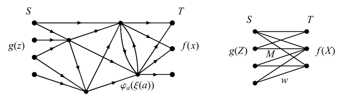
Figure 3: Transformation by a network and a bipartite graph

M^♮-concave functions can be transformed through networks. Let $G=(V,A)$ be a directed graph with two disjoint vertex subsets $S\subseteq V$ and $T\subseteq V$ specified as the entrance and the exit (Fig. 3, left). Suppose that, for each arc $a\in A$, we are given a univariate concave function $\varphi_{a}:\mathbb{Z}\to\mathbb{R}\cup\{-\infty\}$ representing the weight of flow on the arc $a$. Let $\xi\in\mathbb{Z}^{A}$ be a vector representing a flow, and $\partial\xi\in\mathbb{Z}^{V}$ be the boundary of flow $\xi$ defined by (4.36).

Given a function $g:\mathbb{Z}^{S}\to\mathbb{R}\cup\{-\infty\}$ on the entrance set $S$, we define a function $f:\mathbb{Z}^{T}\to\mathbb{R}\cup\{-\infty,+\infty\}$ on the exit set $T$ by

$$f(x)=\sup_{\xi,z}\{g(z)+\sum_{a\in A}\varphi_{a}(\xi(a))\mid\xi\in\mathbb{Z}^{A},\partial\xi=(z,-x,{\bf 0})\in\mathbb{Z}^{S}\times\mathbb{Z}^{T}\times\mathbb{Z}^{V\setminus(S\cup T)}\}\quad(x\in\mathbb{Z}^{T}).$$ (6.7)

This function $f(x)$ represents the maximum weight to meet the demand specification $x$ at the exit, subject to the flow conservation at the vertices not in $S\cup T$. The weight consists of two parts, the weight $g(z)$ of supply $z$ at the entrance $S$ and the weight $\sum_{a\in A}\varphi_{a}(\xi(a))$ in the arcs.

We can regard (6.7) as a transformation of $g$ to $f$ by the network. If the given function $g$ is M^♮-concave, the resultant function $f$ is also M^♮-concave, provided that $f$ does not take the value $+\infty$ and ${\rm dom\,}f$ is nonempty. In other words, the transformation (6.7) by a network preserves M^♮-concavity. See Section 9.6 of Murota (2003) for a proof. An alternative proof is given by Kobayashi et al. (2007).

In particular, an M^♮-concave set function is transformed to another M^♮-concave set function through a bipartite graph (Fig. 3, right). Let $G=(S,T;E)$ be a bipartite graph with vertex bipartition $(S,T)$ and edge set $E$, with weight $w_{e}\in\mathbb{R}$ associated with each edge $e\in E$. Given an M^♮-concave set function $g:2^{S}\to\mathbb{R}\cup\{-\infty\}$ on $S$, define a set function $f$ on $T$ by

$$f(X)=\max\{g(Z)+w(M)\mid\mbox{$M$ is a matching, $S\cap\partial M=Z$, $T\cap\partial M=X$}\}\quad(X\subseteq T),$$ (6.8)

where $f(X)=-\infty$ if no such $M$ exists for $X$. If $g$ is M^♮-concave, then $f$ is also M^♮-concave, as long as ${\rm dom\,}f$ is nonempty. A proof tailored to set functions is given in the proof of Theorem 5.2.18 of Murota (2000a).

6.3 Concluding remarks of section 6

Efficient algorithms are available for the operations listed in Theorem 6.1. In particular, the convolution (6.6), corresponding to the aggregation of utility functions, can be computed efficiently (Murota and Tamura 2003b). The transformation by networks is also accompanied by efficient algorithms. For M^♮-concave function maximization algorithms, see Chapter 10 of Murota (2003), and more recent papers, e.g., Shioura (2004), Tamura (2005), Murota (2010), Moriguchi et al. (2011), Fujishige et al. (2015), and Shioura (2015).

7 Conjugacy and L^♮-convexity

Conjugacy under the Legendre transformation is one of the most appealing facts in convex analysis. This is also the case in discrete convex analysis. The conjugacy theorem in discrete convex analysis says that the Legendre transformation gives a one-to-one correspondence between M^♮-concave functions and L^♮-convex functions. Since M^♮-concavity expresses substitutability of valuation or utility functions, L^♮-convexity characterizes substitutability in terms of indirect utility functions. This fact has a significant application to auction theory, to be expounded in Section 8.

7.1 L^♮-convex function

The concept of L^♮-convexity is defined for functions in discrete (integer) variables and for those in continuous (real) variables. We start with discrete variables.

L^♮-convex function on $\mathbb{Z}^{n}$:

First recall that a function $g:\mathbb{Z}^{n}\to\mathbb{R}\cup\{+\infty\}$ is called submodular if

$$g(p)+g(q)\geq g(p\vee q)+g(p\wedge q)\qquad(p,q\in\mathbb{Z}^{n}),$$ (7.1)

where $p\vee q$ and $p\wedge q$ mean the vectors of componentwise maximum and minimum of $p$ and $q$, respectively. To define L^♮-convexity of $g$, we consider a function $\tilde{g}$ in $n+1$ variables $(p_{0},p)=(p_{0},p_{1},\ldots,p_{n})$ defined as

$$\tilde{g}(p_{0},p)=g(p-p_{0}{\bf 1})\qquad(p_{0}\in\mathbb{Z},p\in\mathbb{Z}^{n}),$$ (7.2)

where $\bm{1}=(1,1,\ldots,1)$. Then we say that $g:\mathbb{Z}^{n}\to\mathbb{R}\cup\{+\infty\}$ is L^♮-convex if the associated function $\tilde{g}:\mathbb{Z}^{n+1}\to\mathbb{R}\cup\{+\infty\}$ is a submodular function in $(p_{0},p)$, i.e., if

$$g(p-p_{0}{\bf 1})+g(q-q_{0}{\bf 1})\geq g((p\vee q)-(p_{0}\vee q_{0}){\bf 1})+g((p\wedge q)-(p_{0}\wedge q_{0}){\bf 1})\quad(p_{0},q_{0}\in\mathbb{Z},p,q\in\mathbb{Z}^{n}).$$ (7.3)

Remark 7.1.

The significance of the extra variable $p_{0}$ in the definition of L^♮-convexity is most transparent when $n=1$. When $n=1$ we have $(p\vee q,p\wedge q)=(p,q)$ or $(q,p)$, according to whether $p\geq q$ or $p\leq q$. Hence the submodular inequality (7.1) is always satisfied, and every function $g:\mathbb{Z}\to\mathbb{R}\cup\{+\infty\}$ is submodular. On the other hand, the inequality (7.3) for $(p_{0},p)=(1,t)$ and $(q_{0},q)=(0,t+1)$ yields $g(t-1)+g(t+1)\geq 2g(t)$ for $t\in\mathbb{Z}$, which shows the convexity of $g$ on $\mathbb{Z}$. The converse is also true. Therefore, a function $g:\mathbb{Z}\to\mathbb{R}\cup\{+\infty\}$ is L^♮-convex if and only if $g(t-1)+g(t+1)\geq 2g(t)$ for all $t\in\mathbb{Z}$.  

Remark 7.2.

For a set function $\mu:2^{N}\to\mathbb{R}\cup\{+\infty\}$, L^♮-convexity is equivalent to submodularity (3.8). Recall the notation $\chi_{X}$ for the characteristic vector of a subset $X$; see (2.1). A set function $\mu$ can be identified with a function $g:\mathbb{Z}^{N}\to\mathbb{R}\cup\{+\infty\}$ with ${\rm dom\,}g\subseteq\{0,1\}^{N}$ by $\mu(X)=g(\chi_{X})$ for $X\subseteq N$, and $\mu$ is submodular if and only if the corresponding $g$ is L^♮-convex.  

Remark 7.3.

Matroid rank functions have a dual character of being both L^♮-convex and M^♮-concave. It is L^♮-convex as it is submodular, and M^♮-concave as already mentioned in Section 3.6.  

L^♮-convexity can be characterized by a number of equivalent conditions (Favati and Tardella 1990, Fujishige and Murota 2000, Murota 2003).

Theorem 7.1.

For $g:\mathbb{Z}^{n}\to\mathbb{R}\cup\{+\infty\}$ the following conditions, (a) to (d), are equivalent:

(a) L^♮-convexity, i.e., (7.3).

(b) Translation-submodularity:

$$g(p)+g(q)\geq g((p-\alpha{\bf 1})\vee q)+g(p\wedge(q+\alpha{\bf 1}))\qquad(\forall p,q\in\mathbb{Z}^{n},\forall\alpha\in\mathbb{Z}_{+}).$$ (7.4)

(c) Discrete midpoint convexity:

$$g(p)+g(q)\geq g\left(\left\lceil\frac{p+q}{2}\right\rceil\right)+g\left(\left\lfloor\frac{p+q}{2}\right\rfloor\right)\qquad(p,q\in\mathbb{Z}^{n}),$$ (7.5)

where $\lceil\cdot\rceil$ and $\lfloor\cdot\rfloor$ denote the integer vectors obtained by componentwise rounding-up and rounding-down to the nearest integers, respectively.

(d) For any $p,q\in\mathbb{Z}^{n}$ with ${\rm supp}^{+}(p-q)\not=\emptyset$, it holds that

$$g(p)+g(q)\geq g(p-\chi_{A})+g(q+\chi_{A}),$$ (7.6)

where $\displaystyle A=\arg\max_{i}\{p_{i}-q_{i}\}$.

It is known (Theorem 7.20 of Murota 2003) that an L^♮-convex function $g:\mathbb{Z}^{n}\to\mathbb{R}\cup\{+\infty\}$ is convex-extensible, i.e., there exists a convex function $\overline{g}:\mathbb{R}^{n}\to\mathbb{R}\cup\{+\infty\}$ such that $\overline{g}(p)=g(p)$ for all $p\in\mathbb{Z}^{n}$. Moreover, the convex extension $\overline{g}$ can be constructed by a simple procedure; see Theorem 7.19 of Murota (2003).

Remark 7.4.

A nonempty set $P\subseteq\mathbb{Z}^{n}$ is called an L^♮-convex set if its indicator function is an L^♮-convex function. In other words, $P\not=\emptyset$ is an L^♮-convex set if it satisfies one of the following equivalent conditions, where $p,q\in\mathbb{Z}^{n}$ and $p_{0},q_{0}\in\mathbb{Z}$:

• $p-p_{0}{\bf 1},\ q-q_{0}{\bf 1}\ \in P$  $\Longrightarrow$  $(p\vee q)-(p_{0}\vee q_{0}){\bf 1},\ (p\wedge q)-(p_{0}\wedge q_{0}){\bf 1}\ \in P$.

• $p,q\in P$, $\alpha\in\mathbb{Z}_{+}$  $\Longrightarrow$  $(p-\alpha{\bf 1})\vee q,\ p\wedge(q+\alpha{\bf 1})\ \in P$.

• $p,q\in P$  $\Longrightarrow$  $\left\lceil\frac{p+q}{2}\right\rceil,\ \left\lfloor\frac{p+q}{2}\right\rfloor\ \in P$.

• $p,q\in P$,   ${\rm supp}^{+}(p-q)\not=\emptyset$  $\Longrightarrow$  $p-\chi_{A},\ q+\chi_{A}\ \in P$ with $\displaystyle A=\arg\max_{i}\{p_{i}-q_{i}\}$.

For an L^♮-convex function $g$, the effective domain ${\rm dom\,}g$ and the set of minimizers $\arg\min g$ are L^♮-convex sets. See Section 5.5 of Murota (2003) for more about L^♮-convex sets.  

Remark 7.5.

A function $g:\mathbb{Z}^{n}\to\mathbb{R}\cup\{+\infty\}$ is called an L-convex function if it is an L^♮-convex function such that there exists $r\in\mathbb{R}$ for which $g(p+{\bf 1})=g(p)+r$ for all $p\in\mathbb{Z}^{n}$. L-convex functions and L^♮-convex functions are equivalent concepts, in that L^♮-convex functions in $n$ variables can be identified, up to the constant $r$, with L-convex functions in $n+1$ variables. Indeed, a function $g:\mathbb{Z}^{n}\to\mathbb{R}\cup\{+\infty\}$ is L^♮-convex if and only if the function $\tilde{g}:\mathbb{Z}^{n+1}\to\mathbb{R}\cup\{+\infty\}$ in (7.2) is an L-convex function (with $r=0$).  

L^♮-convex function on $\mathbb{R}^{n}$:

We turn to continuous variables. A function $g:\mathbb{R}^{n}\to\mathbb{R}\cup\{+\infty\}$ is said to be L^♮-convex if it is a convex function (in the ordinary sense) such that $\tilde{g}(p_{0},p)=g(p-p_{0}{\bf 1})$ $(p_{0}\in\mathbb{R},p\in\mathbb{R}^{n})$ is a submodular function in $n+1$ variables, i.e.,

$$g(p-p_{0}{\bf 1})+g(q-q_{0}{\bf 1})\geq g((p\vee q)-(p_{0}\vee q_{0}){\bf 1})+g((p\wedge q)-(p_{0}\wedge q_{0}){\bf 1})\quad(p_{0},q_{0}\in\mathbb{R},p,q\in\mathbb{R}^{n}).$$ (7.7)

In the following we restrict ourselves to closed proper L^♮-convex functions, for which the closure of the effective domain ${\rm dom\,}g$ is a well-behaved polyhedron (L^♮-convex polyhedron); see Theorem 3.3 of Murota and Shioura (2008). For a closed proper convex function $g:\mathbb{R}^{n}\to\mathbb{R}\cup\{+\infty\}$, the condition (7.7) for L^♮-convexity is equivalent to translation-submodularity:

$$g(p)+g(q)\geq g((p-\alpha{\bf 1})\vee q)+g(p\wedge(q+\alpha{\bf 1}))\qquad(\forall p,q\in\mathbb{R}^{n},\forall\alpha\in\mathbb{R}_{+}).$$ (7.8)

Often we are interested in polyhedral L^♮-convex functions.

L^♮-convex functions in real variables are investigated by Murota and Shioura (2000, 2004a, 2004b, 2008).

7.2 Conjugacy

Functions in continuous variables:

For a function $f:\mathbb{R}^{n}\to\mathbb{R}\cup\{+\infty\}$ (not necessarily convex) with ${\rm dom\,}f\not=\emptyset$, the convex conjugate $f^{\bullet}:\mathbb{R}^{n}\to\mathbb{R}\cup\{+\infty\}$ is defined by

$$f^{\bullet}(p)=\sup\{\langle p,x\rangle-f(x)\mid x\in\mathbb{R}^{n}\}\qquad(p\in\mathbb{R}^{n}),$$ (7.9)

where $\langle p,x\rangle=\sum_{i=1}^{n}p_{i}x_{i}$ is the inner product of $p=(p_{i})\in\mathbb{R}^{n}$ and $x=(x_{i})\in\mathbb{R}^{n}$. The function $f^{\bullet}$ is also referred to as the (convex) Legendre(–Fenchel) transform of $f$, and the mapping $f\mapsto f^{\bullet}$ as the (convex) Legendre(–Fenchel) transformation. A fundamental theorem in convex analysis states that the Legendre transformation gives a symmetric one-to-one correspondence in the class of all closed proper convex functions. That is, for a closed proper convex function $f$, the conjugate function $f^{\bullet}$ is a closed proper convex function and the biconjugacy $(f^{\bullet})^{\bullet}=f$ holds.

To formulate the correspondence between concave functions $f:\mathbb{R}^{n}\to\mathbb{R}\cup\{-\infty\}$ and convex functions $g:\mathbb{R}^{n}\to\mathbb{R}\cup\{+\infty\}$ with ${\rm dom\,}f\not=\emptyset$ and ${\rm dom\,}g\not=\emptyset$, we introduce the following variants of the transformation (7.9):

$$f^{\triangledown}(p) =\sup\{f(x)-\langle p,x\rangle\mid x\in\mathbb{R}^{n}\}\qquad(p\in\mathbb{R}^{n}),$$ (7.10)

$$g^{\triangle}(x) =\inf\{g(p)+\langle p,x\rangle\mid p\in\mathbb{R}^{n}\}\qquad(x\in\mathbb{R}^{n}),$$ (7.11)

where $f^{\triangledown}:\mathbb{R}^{n}\to\mathbb{R}\cup\{+\infty\}$ and $g^{\triangle}:\mathbb{R}^{n}\to\mathbb{R}\cup\{-\infty\}$. The biconjugacy is expressed as $(f^{\triangledown})^{\triangle}=f$, $(g^{\triangle})^{\triangledown}=g$ for closed proper concave functions $f$ and closed proper convex functions $g$.

Theorem 7.2.

(1) The transformations (7.10) and (7.11) give a one-to-one correspondence between the classes of all closed proper concave functions $f$ and closed proper convex functions $g$.

(2) For a closed proper concave function $f:\mathbb{R}^{n}\to\mathbb{R}\cup\{-\infty\}$, the conjugate function $f^{\triangledown}:\mathbb{R}^{n}\to\mathbb{R}\cup\{+\infty\}$ is a closed proper convex function and $(f^{\triangledown})^{\triangle}=f$.

(3) For a closed proper convex function $g:\mathbb{R}^{n}\to\mathbb{R}\cup\{+\infty\}$, the conjugate function $g^{\triangle}:\mathbb{R}^{n}\to\mathbb{R}\cup\{-\infty\}$ is a closed proper concave function and $(g^{\triangle})^{\triangledown}=g$.

Addition of combinatorial ingredients to the above theorem yields the conjugacy theorem between M^♮-concave and L^♮-convex functions (Murota and Shioura 2004a).

Theorem 7.3.

(1) The transformations (7.10) and (7.11) give a one-to-one correspondence between the classes of all closed proper M^♮-concave functions $f$ and closed proper L^♮-convex functions $g$.

(2) For a closed proper M^♮-concave function $f:\mathbb{R}^{n}\to\mathbb{R}\cup\{-\infty\}$, the conjugate function $f^{\triangledown}:\mathbb{R}^{n}\to\mathbb{R}\cup\{+\infty\}$ is a closed proper L^♮-convex function and $(f^{\triangledown})^{\triangle}=f$.

(3) For a closed proper L^♮-convex function $g:\mathbb{R}^{n}\to\mathbb{R}\cup\{+\infty\}$, the conjugate function $g^{\triangle}:\mathbb{R}^{n}\to\mathbb{R}\cup\{-\infty\}$ is a closed proper M^♮-concave function and $(g^{\triangle})^{\triangledown}=g$.

The M^♮/L^♮-conjugacy is also valid for polyhedral concave/convex functions (Murota and Shioura 2000, Theorem 8.4 of Murota 2003).

Theorem 7.4.

(1) The transformations (7.10) and (7.11) give a one-to-one correspondence between the classes of all polyhedral M^♮-concave functions $f$ and polyhedral L^♮-convex functions $g$.

(2) For a polyhedral M^♮-concave function $f:\mathbb{R}^{n}\to\mathbb{R}\cup\{-\infty\}$, the conjugate function $f^{\triangledown}:\mathbb{R}^{n}\to\mathbb{R}\cup\{+\infty\}$ is a polyhedral L^♮-convex function and $(f^{\triangledown})^{\triangle}=f$.

(3) For a polyhedral L^♮-convex function $g:\mathbb{R}^{n}\to\mathbb{R}\cup\{+\infty\}$, the conjugate function $g^{\triangle}:\mathbb{R}^{n}\to\mathbb{R}\cup\{-\infty\}$ is a polyhedral M^♮-concave function and $(g^{\triangle})^{\triangledown}=g$.

As corollaries of the conjugacy theorems, the following characterizations of M^♮-concavity and L^♮-convexity in terms of the conjugate functions are obtained.

Theorem 7.5.

(1) A function $f:\mathbb{R}^{n}\to\mathbb{R}\cup\{-\infty\}$ is closed proper M^♮-concave if and only if the conjugate function $f^{\triangledown}:\mathbb{R}^{n}\to\mathbb{R}\cup\{+\infty\}$ by (7.10) is closed proper L^♮-convex.

(2) A function $f:\mathbb{R}^{n}\to\mathbb{R}\cup\{-\infty\}$ is polyhedral M^♮-concave if and only if the conjugate function $f^{\triangledown}:\mathbb{R}^{n}\to\mathbb{R}\cup\{+\infty\}$ by (7.10) is polyhedral L^♮-convex.

Theorem 7.6.

(1) A function $g:\mathbb{R}^{n}\to\mathbb{R}\cup\{+\infty\}$ is closed proper L^♮-convex if and only if the conjugate function $g^{\triangle}:\mathbb{R}^{n}\to\mathbb{R}\cup\{-\infty\}$ by (7.11) is closed proper M^♮-concave.

(2) A function $g:\mathbb{R}^{n}\to\mathbb{R}\cup\{+\infty\}$ is polyhedral L^♮-convex if and only if the conjugate function $g^{\triangle}:\mathbb{R}^{n}\to\mathbb{R}\cup\{-\infty\}$ by (7.11) is polyhedral M^♮-concave.

L^♮-convexity, being equivalent to translation-submodularity, is a stronger property than mere submodularity. When we replace L^♮-convexity of $f^{\triangledown}$ in Theorem 7.5 (2) with submodularity, we obtain a larger class of polyhedral concave functions $f$ than M^♮-concave functions. The following theorem is ascribed to Danilov and Lang (2001) in Danilov et al. (2003); see also Appendix of Shioura and Tamura (2015) for technical supplements.

Theorem 7.7.

Let $f:\mathbb{R}^{N}\to\mathbb{R}\cup\{-\infty\}$ be a polyhedral concave function with a bounded effective domain. Then the following conditions are equivalent:

(a) $f$ satisfies (GS[$\mathbb{R}$]).

(b) For every $p\in\mathbb{R}^{N}$, each edge (one-dimensional face) of $D(p;f)$ is parallel to a vector $d$ with $|{\rm supp}^{+}(d)|\leq 1$ and $|{\rm supp}^{-}(d)|\leq 1$.

(c) $f^{\triangledown}:\mathbb{R}^{N}\to\mathbb{R}\cup\{+\infty\}$ by (7.10) is a submodular function.

Remark 7.6.

In Danilov et al. (2003) a bounded polyhedron $P$ is called a quasi-polymatroid if each edge (one-dimensional face) is parallel to a vector $d$ with $|{\rm supp}^{+}(d)|\leq 1$ and $|{\rm supp}^{-}(d)|\leq 1$. It follows from Theorem 3.1 of Fujishige et al. (2004) that every face of a quasi-polymatroid whose normal vector has the full support $N$ is obtained from an M-convex polyhedron (base polyhedron) by a scaling along axes. We mention in passing that a pointed convex polyhedron is called polybasic if each edge is parallel to a vector $d$ with $|{\rm supp}^{+}(d)|+|{\rm supp}^{-}(d)|\leq 2$ (Fujishige et al. 2004).  

Remark 7.7.

In the canonical situation, where $f:\mathbb{R}^{n}\to\mathbb{R}$ is a strictly concave smooth function, the equivalence between (GS[$\mathbb{R}$]) of $f$ and the submodularity of $g=f^{\triangledown}$ is easily derived by simple calculus. Let $x(p)$ be the unique maximizer of $f(x)-\langle p,x\rangle$. We have $p_{i}=\partial f/\partial x_{i}$ for $i=1,\ldots,n$, and $g(p)=f(x(p))-\langle p,x(p)\rangle$. This implies $\partial g/\partial p_{i}=-x_{i}$ $(i=1,\ldots,n)$, and hence $\partial^{2}g/\partial p_{i}\partial p_{j}=-\partial x_{i}/\partial p_{j}$ $(i,j=1,\ldots,n)$. On the other hand, the submodularity of $g$ is equivalent to $\partial^{2}g/\partial p_{i}\partial p_{j}\leq 0$ $(i\not=j)$, and (GS[$\mathbb{R}$]) of $f$ is represented as $\partial x_{i}/\partial p_{j}\geq 0$ $(i\not=j)$.  

Functions in discrete variables:

We turn to functions defined on integer vectors. For functions $f:\mathbb{Z}^{n}\to\mathbb{R}\cup\{-\infty\}$ and $g:\mathbb{Z}^{n}\to\mathbb{R}\cup\{+\infty\}$ with ${\rm dom\,}f\not=\emptyset$ and ${\rm dom\,}g\not=\emptyset$, the transformations (7.10) and (7.11) are modified to

$$f^{\triangledown}(p) =\sup\{f(x)-\langle p,x\rangle\mid x\in\mathbb{Z}^{n}\}\qquad(p\in\mathbb{R}^{n}),$$ (7.12)

$$g^{\triangle}(x) =\inf\{g(p)+\langle p,x\rangle\mid p\in\mathbb{Z}^{n}\}\qquad(x\in\mathbb{R}^{n}),$$ (7.13)

where $f^{\triangledown}:\mathbb{R}^{n}\to\mathbb{R}\cup\{+\infty\}$ and $g^{\triangle}:\mathbb{R}^{n}\to\mathbb{R}\cup\{-\infty\}$.

The conjugacy between M^♮-concavity and L^♮-convexity in this case reads as follows.

Theorem 7.8.

(1) For an M^♮-concave function $f:\mathbb{Z}^{n}\to\mathbb{R}\cup\{-\infty\}$, the conjugate function $f^{\triangledown}:\mathbb{R}^{n}\to\mathbb{R}\cup\{+\infty\}$ is a (locally polyhedral) L^♮-convex function, and $(f^{\triangledown})^{\triangle}(x)=f(x)$ for $x\in\mathbb{Z}^{n}$.

(2) For an L^♮-convex function $g:\mathbb{Z}^{n}\to\mathbb{R}\cup\{+\infty\}$, the conjugate function $g^{\triangle}:\mathbb{R}^{n}\to\mathbb{R}\cup\{-\infty\}$ is a (locally polyhedral) M^♮-concave function, and $(g^{\triangle})^{\triangledown}(p)=g(p)$ for $p\in\mathbb{Z}^{n}$.

For integer-valued functions $f$ and $g$, $f^{\triangledown}(p)$ and $g^{\triangle}(x)$ are integers for integer vectors $p$ and $x$. Hence (7.12) with $p\in\mathbb{Z}^{n}$ and (7.13) with $x\in\mathbb{Z}^{n}$, i.e.,

$$f^{\triangledown}(p) =\sup\{f(x)-\langle p,x\rangle\mid x\in\mathbb{Z}^{n}\}\qquad(p\in\mathbb{Z}^{n}),$$ (7.14)

$$g^{\triangle}(x) =\inf\{g(p)+\langle p,x\rangle\mid p\in\mathbb{Z}^{n}\}\qquad(x\in\mathbb{Z}^{n}),$$ (7.15)

define transformations of $f:\mathbb{Z}^{n}\to\mathbb{Z}\cup\{-\infty\}$ to $f^{\triangledown}:\mathbb{Z}^{n}\to\mathbb{Z}\cup\{+\infty\}$ and $g:\mathbb{Z}^{n}\to\mathbb{Z}\cup\{+\infty\}$ to $g^{\triangle}:\mathbb{Z}^{n}\to\mathbb{Z}\cup\{-\infty\}$, respectively.

The conjugacy theorem for integer-valued discrete-variable M^♮-concave and L^♮-convex functions reads as follows (Murota 1998, Theorem 8.12 of Murota 2003).

Theorem 7.9.

(1) The transformations (7.14) and (7.15) give a one-to-one correspondence between the classes of all integer-valued M^♮-concave functions $f$ and integer-valued L^♮-convex functions $g$.

(2) For an integer-valued M^♮-concave function $f:\mathbb{Z}^{n}\to\mathbb{Z}\cup\{-\infty\}$, the conjugate function $f^{\triangledown}:\mathbb{Z}^{n}\to\mathbb{Z}\cup\{+\infty\}$ is an integer-valued L^♮-convex function and $(f^{\triangledown})^{\triangle}=f$.

(3) For an integer-valued L^♮-convex function $g:\mathbb{Z}^{n}\to\mathbb{Z}\cup\{+\infty\}$, the conjugate function $g^{\triangle}:\mathbb{Z}^{n}\to\mathbb{Z}\cup\{-\infty\}$ is an integer-valued M^♮-concave function and $(g^{\triangle})^{\triangledown}=g$.

As corollaries of the conjugacy theorems, the following characterizations of M^♮-concavity and L^♮-convexity in terms of the conjugate functions are obtained.

Theorem 7.10.

(1) A function $f:\mathbb{Z}^{n}\to\mathbb{R}\cup\{-\infty\}$ is M^♮-concave if and only if the conjugate function $f^{\triangledown}:\mathbb{R}^{n}\to\mathbb{R}\cup\{+\infty\}$ by (7.12) is (locally polyhedral) L^♮-convex.

(2) A function $f:\mathbb{Z}^{n}\to\mathbb{Z}\cup\{-\infty\}$ is M^♮-concave if and only if the conjugate function $f^{\triangledown}:\mathbb{Z}^{n}\to\mathbb{Z}\cup\{+\infty\}$ by (7.14) is L^♮-convex.

Theorem 7.11.

(1) A function $g:\mathbb{Z}^{n}\to\mathbb{R}\cup\{+\infty\}$ is L^♮-convex if and only if the conjugate function $g^{\triangle}:\mathbb{R}^{n}\to\mathbb{R}\cup\{-\infty\}$ by (7.13) is (locally polyhedral) M^♮-concave.

(2) A function $g:\mathbb{Z}^{n}\to\mathbb{Z}\cup\{+\infty\}$ is L^♮-convex if and only if the conjugate function $g^{\triangle}:\mathbb{Z}^{n}\to\mathbb{Z}\cup\{-\infty\}$ by (7.15) is M^♮-concave.

L^♮-convexity, being equivalent to translation-submodularity, is a stronger property than mere submodularity. Naturally, we may wonder if L^♮-convexity of $f^{\triangledown}$ in Theorem 7.10 can be replaced by submodularity. However, the following example denies this possibility.

Example 7.1.

Here is an example of a function $f$ such that the conjugate function $f^{\triangledown}$ is submodular, but $f$ is not M^♮-concave. Let $f:\mathbb{Z}^{2}\to\mathbb{R}\cup\{-\infty\}$ be defined by $f(x_{1},x_{2})=\min(2,x_{1}+2x_{2})$ on ${\rm dom\,}f=\{(x_{1},x_{2})\in\mathbb{Z}^{2}\mid 0\leq x_{1}\leq 2,0\leq x_{2}\leq 1\}$, whose numerical values are

$$f(0,0)=0,\ f(1,0)=1,\ f(2,0)=2;\quad f(0,1)=f(1,1)=f(2,1)=2.$$

This function is not M^♮-concave because (M^♮-EXC[$\mathbb{Z}$]) fails for $x=(2,0)$, $y=(0,1)$ and $i=1$. The conjugate function $f^{\triangledown}:\mathbb{R}^{2}\to\mathbb{R}\cup\{+\infty\}$ of (7.12) is given by

$$f^{\triangledown}(p_{1},p_{2})=\max(0,2-2p_{1},2-p_{2},2-2p_{1}-p_{2})=\left\{\begin{array}[]{ll}0&(p_{1}\geq 1,p_{2}\geq 2),\\ 2-2p_{1}&(2p_{1}\leq\min(2,p_{2}),p_{2}\geq 0),\\ 2-p_{2}&(p_{2}\leq\min(2,2p_{1}),p_{1}\geq 0),\\ 2-2p_{1}-p_{2}&(p_{1}\leq 0,p_{2}\leq 0).\\ \end{array}\right.$$

The function $f^{\triangledown}$ is submodular, as is easily verified, but it is not L^♮-convex since the translation-submodularity (7.8) fails for $g=f^{\triangledown}$, $p=(1,2)$, $q=(0,0)$ and $\alpha=1$ with $g(p)+g(q)=0+2=2$ and $g((p-\alpha{\bf 1})\vee q)+g(p\wedge(q+\alpha{\bf 1}))=g(0,1)+g(1,1)=2+1=3$. It is also noted that $f^{\triangledown}(p_{1}/2,p_{2})$ is L^♮-convex in $(p_{1},p_{2})$.  

In spite of the above example, M^♮-concavity of a set function $f:2^{N}\to\mathbb{R}\cup\{-\infty\}$ can be characterized by submodularity of the conjugate function $f^{\triangledown}$, which is defined by

$$f^{\triangledown}(p) =\max\{f(X)-p(X)\mid X\subseteq N\}\qquad(p\in\mathbb{R}^{n})$$ (7.16)

as an adaptation of (7.12).

Theorem 7.12.

A set function $f:2^{N}\to\mathbb{R}\cup\{-\infty\}$ is M^♮-concave if and only if the conjugate function $f^{\triangledown}:\mathbb{R}^{n}\to\mathbb{R}\cup\{+\infty\}$ in (7.16) is submodular.

This theorem can be derived from a combination of Theorem 10 of Ausubel and Milgrom (2002) with Theorem 3.7 in Section 3.3; see also Section 7.2.2 of Shioura and Tamura (2015) for an alternative proof.

7.3 Minimization of L^♮-convex functions

The set of the minimizers of an L^♮-convex function on $\mathbb{Z}^{n}$ forms a well-behaved “discrete convex” subset of $\mathbb{Z}^{n}$. Recall from Remark 7.4 that a nonempty set $P\subseteq\mathbb{Z}^{n}$ is called an L^♮-convex set if

$$p,q\in P\ \Longrightarrow\ (p-\alpha{\bf 1})\vee q,\ p\wedge(q+\alpha{\bf 1})\in P\qquad(\forall\alpha\in\mathbb{Z}_{+}).$$ (7.17)

This condition with $\alpha=0$ gives

$$p,q\in P\ \Longrightarrow\ p\vee q,\ p\wedge q\in P,$$ (7.18)

which shows that an L^♮-convex set forms a sublattice of $\mathbb{Z}^{n}$. A bounded L^♮-convex set has the (uniquely determined) maximal element and the (uniquely determined) minimal element.

Theorem 7.13.

Let $g:\mathbb{Z}^{N}\to\mathbb{R}\cup\{+\infty\}$ be an L^♮-convex function and assume $\arg\min g\not=\emptyset$. Then the set of the minimizers $\arg\min g$ is an L^♮-convex set. If $\arg\min g$ is bounded, there exist the maximal and the minimal minimizer of $g$.

Proof.

This follows easily from the translation-submodularity in Theorem 7.1 (b). ∎

For an L^♮-convex function, the minimality of a function value is characterized by a local condition as follows (Theorem 7.14 of Murota 2003). Recall the notation $\chi_{Y}$ for the characteristic vector of a subset $Y$; see (2.1).

Theorem 7.14.

Let $g:\mathbb{Z}^{N}\to\mathbb{R}\cup\{+\infty\}$ be an L^♮-convex function and $p\in{\rm dom\,}g$.

(1) If $g(p)>g(q)$ for $q\in{\rm dom\,}g$, then $g(p)>g(p+\chi_{Y})$ for some $Y\subseteq{\rm supp}^{+}(q-p)$ or $g(p)>g(p-\chi_{Z})$ for some $Z\subseteq{\rm supp}^{-}(q-p)$.

(2) $p$ is a minimizer of $g$ if and only if

$$g(p)\leq g(p+\chi_{Y})\quad(\forall\,Y\subseteq N),\qquad g(p)\leq g(p-\chi_{Z})\quad(\forall\,Z\subseteq N).$$ (7.19)

Proof.

(1) This follows from Theorem 7.15 below. If $g(q)<g(p)$ in (7.20), $g(p+\chi_{Y_{k}})-g(p)<0$ for some $k$ or $g(p-\chi_{Z_{j}})-g(p)<0$ for some $j$. (2) This is immediate from (1). ∎

Theorem 7.15.

Let $g:\mathbb{Z}^{N}\to\mathbb{R}\cup\{+\infty\}$ be an L^♮-convex function. For $p,q\in{\rm dom\,}g$ we have

$$g(q)\geq g(p)+\sum_{k=1}^{m}[g(p+\chi_{Y_{k}})-g(p)]+\sum_{j=1}^{l}[g(p-\chi_{Z_{j}})-g(p)],$$ (7.20)

where $\emptyset\not=Y_{1}\subseteq Y_{2}\subseteq\cdots\subseteq Y_{m}={\rm supp}^{+}(q-p)$,  $\emptyset\not=Z_{1}\subseteq Z_{2}\subseteq\cdots\subseteq Z_{l}={\rm supp}^{-}(q-p)$, and

$$q-p=\sum_{k=1}^{m}\chi_{Y_{k}}-\sum_{j=1}^{l}\chi_{Z_{j}}.$$ (7.21)

Proof.

(1) If ${\rm supp}^{+}(q-p)$ is nonempty, (7.6) for $(q,p)$ implies

$$g(q)\geq g(p+\chi_{Y_{1}})+g(q-\chi_{Y_{1}})-g(p)=[g(p+\chi_{Y_{1}})-g(p)]+g(q_{2}),$$

where $q_{2}=q-\chi_{Y_{1}}$. If ${\rm supp}^{+}(q_{2}-p)$ is nonempty, (7.6) for $(q_{2},p)$ implies

$$g(q_{2})\geq g(p+\chi_{Y_{2}})+g(q_{2}-\chi_{Y_{2}})-g(p)=[g(p+\chi_{Y_{2}})-g(p)]+g(q_{3}),$$

where $q_{3}=q_{2}-\chi_{Y_{2}}=q-\chi_{Y_{1}}-\chi_{Y_{2}}$. Repeating this, we obtain $q^{\prime}=q-\sum_{k=1}^{m}\chi_{Y_{k}}=p\wedge q$ and

$$g(q)\geq g(q^{\prime})+\sum_{k=1}^{m}[g(p+\chi_{Y_{k}})-g(p)].$$ (7.22)

By the similar procedure starting with $(p,q^{\prime})$ we obtain $p=q^{\prime}+\sum_{j=1}^{l}\chi_{Z_{j}}$ and

$$g(q^{\prime})\geq g(p)+\sum_{j=1}^{l}[g(p-\chi_{Z_{j}})-g(p)].$$ (7.23)

Adding (7.22) and (7.23) we obtain (7.20). ∎

Algorithms for L^♮-convex minimization:

Algorithms for L^♮-convex function minimization are considered by Murota (2000b), Kolmogorov and Shioura (2009), Murota and Shioura (2014, 2017), Murota et al. (2016), and Shioura (2017); see also Section 10.3 of Murota (2003). Among others we present here the following two algorithms.

Algorithm Greedy

Step 0: Find a vector $p^{\circ}\in{\rm dom\,}g$   and set $p:=p^{\circ}$.

Step 1: Find $\varepsilon\in\{+1,-1\}$ and $X\subseteq N$ that minimize $g(p+\varepsilon\chi_{X})$.

Step 2: If $g(p)\leq g(p+\varepsilon\chi_{X})$, then output $p$ and stop.

Step 3: Set $p:=p+\varepsilon\chi_{X}$  and  go to Step 1.

Algorithm GreedyUpMinimal

Step 0: Find a vector $p^{\circ}\in{\rm dom\,}g$ such that $\{q\mid q\geq p^{\circ}\}\cap\arg\min g\not=\emptyset$    and set $p:=p^{\circ}$.

Step 1: Find the minimal minimizer $X\subseteq N$ of $g(p+\chi_{X})$.

Step 2: If $X=\emptyset$, then output $p$ and stop.

Step 3: Set $p:=p+\chi_{X}$  and  go to Step 1.

The algorithm Greedy can start with an arbitrary initial vector $p^{\circ}$ in the effective domain, and the vector $p$ may increase or decrease depending on $\varepsilon=+1$ or $-1$. The output of the algorithm Greedy is not uniquely determined, varying with the choice of $\varepsilon$ and $X$ in case of ties in minimizing $g(p+\varepsilon\chi_{X})$ in Step 1. Step 1 amounts to minimizing two set functions $\rho_{+}(X)=g(p+\chi_{X})-g(p)$ and $\rho_{-}(X)=g(p-\chi_{X})-g(p)$ over all subsets $X$ of $N$. As a consequence of submodularity of $g$, both $\rho_{+}$ and $\rho_{-}$ are submodular set functions and they can be minimized efficiently (i.e., in strongly polynomial time). The second algorithm, GreedyUpMinimal, keeps increasing the vector $p$, until it reaches the smallest minimizer of $g$ that is greater than or equal to $p^{\circ}$. Accordingly, the initial vector $p^{\circ}$ must be small enough to ensure $\{q\mid q\geq p^{\circ}\}\cap\arg\min g\not=\emptyset$. If $g$ has the minimal minimizer $p^{*}_{\min}$ and $p^{\circ}\leq p^{*}_{\min}$, then the algorithm GreedyUpMinimal outputs $p^{*}_{\min}$.

The correctness of the algorithms, at their termination, is guaranteed by Theorem 7.14, whereas the following exact bounds for the number of updates of $p$ are established recently by Murota and Shioura (2014).

Theorem 7.16.

(1) The number of updates of $p$ in the algorithm Greedy is exactly equal to

$$\mu(p^{\circ})=\min\{\|p^{\circ}-p^{*}\|_{\infty}^{+}+\|p^{\circ}-p^{*}\|_{\infty}^{-}\mid p^{*}\in\arg\min g\}$$ (7.24)

under the assumption of $\arg\min g\not=\emptyset$, where $\|q\|_{\infty}^{+}=\max(0,q_{1},q_{2},\ldots,q_{n})$ and $\|q\|_{\infty}^{-}=\max(0,-q_{1},-q_{2},\ldots,-q_{n})$.

(2) The number of updates of $p$ in the algorithm GreedyUpMinimal is exactly equal to

$$\hat{\mu}(p^{\circ})=\min\{\|p^{\circ}-p^{*}\|_{\infty}\mid p^{*}\in\arg\min g,\ p^{\circ}\leq p^{*}\}$$ (7.25)

under the assumption of $\{q\mid q\geq p^{\circ}\}\cap\arg\min g\not=\emptyset$. If the minimal minimizer $p^{*}_{\min}$ exists and $p^{\circ}\leq p^{*}_{\min}$, then $\hat{\mu}(p^{\circ})=\|p^{\circ}-p^{*}_{\min}\|_{\infty}$.

We can conceive variants of GreedyUpMinimal by changing “Up” to “Down” and/or “Minimal” to “Maximal” according to Table 1 (a). For example, the algorithm GreedyDownMinimal is obtained from GreedyUpMinimal by changing Steps 0 and 1 to:

Step 0: Find a vector $p^{\circ}\in{\rm dom\,}g$ such that $\{q\mid q\leq p^{\circ}\}$ $\cap\arg\min g\not=\emptyset$    and set $p:=p^{\circ}$.

Step 1: Find the maximal minimizer $X\subseteq N$ of $g(p-\chi_{X})$.

Starting with an initial vector $p^{\circ}$ large enough to ensure $\{q\mid q\leq p^{\circ}\}\cap\arg\min g\not=\emptyset$, this algorithm keeps decreasing the vector $p$. If $g$ has the minimal minimizer $p^{*}_{\min}$, the algorithm stops when it reaches $p^{*}_{\min}$. The number of updates of $p$ in GreedyDownMinimal is exactly equal to $\|p^{\circ}-p^{*}_{\min}\|_{\infty}$ (Proposition 3.7 of Murota et al. 2016). Table 1 (b) shows the output and the number of updates of $p$ for the four algorithms.

Table 1: Algorithms Greedy-{Up, Down}-{Minimal, Maximal}

(a) Description of the algorithms

Greedy		Minimal	Maximal
Up	Step 0	$p^{\circ}$ such that  $\{q\mid q\geq p^{\circ}\}\cap\arg\min g\not=\emptyset$  (i.e., $p^{*}_{\max}\geq p^{\circ}$)
	Step 1	minimal minimizer $X$ of $g(p+\chi_{X})$	maximal minimizer $X$ of $g(p+\chi_{X})$
Down	Step 0	$p^{\circ}$ such that  $\{q\mid q\leq p^{\circ}\}\cap\arg\min g\not=\emptyset$  (i.e., $p^{*}_{\min}\leq p^{\circ}$)
	Step 1	maximal minimizer $X$ of $g(p-\chi_{X})$	minimal minimizer $X$ of $g(p-\chi_{X})$
(b) Output and the exact number of updates of $p$
Greedy		Minimal	Maximal
Up	Output	$p^{*}_{\min}$ if $p^{*}_{\min}\geq p^{\circ}$; otherwise	$p^{*}_{\max}$
		$\min(\{q\mid q\geq p^{\circ}\}\cap\arg\min g)$
# Updates		$\|p^{\circ}-p^{*}_{\min}\|_{\infty}$ if $p^{*}_{\min}\geq p^{\circ}$;	$\|p^{\circ}-p^{*}_{\max}\|_{\infty}$
		otherwise $\hat{\mu}(p^{\circ})$
Down	Output	$p^{*}_{\min}$	$p^{*}_{\max}$ if $p^{*}_{\max}\leq p^{\circ}$; otherwise
			$\max(\{q\mid q\leq p^{\circ}\}\cap\arg\min g)$
# Updates		$\|p^{\circ}-p^{*}_{\min}\|_{\infty}$	$\|p^{\circ}-p^{*}_{\max}\|_{\infty}$ if $p^{*}_{\max}\leq p^{\circ}$;
			otherwise $\check{\mu}(p^{\circ})$
$p^{\circ}$: initial vector,   $p^{*}_{\min}$: minimal minimizer of $g$,   $p^{*}_{\max}$: maximal minimizer of $g$
$\hat{\mu}(p^{\circ})=\min\{\|p^{\circ}-p^{*}\|_{\infty}\mid p^{*}\in\arg\min g,\ p^{\circ}\leq p^{*}\}$
$\check{\mu}(p^{\circ})=\min\{\|p^{\circ}-p^{*}\|_{\infty}\mid p^{*}\in\arg\min g,\ p^{\circ}\geq p^{*}\}$

In Section 8 we shall discuss connection of L^♮-convex function minimization to iterative auctions. The algorithm GreedyUpMinimal corresponds to ascending (English) auctions, and GreedyDownMaximal to descending (Dutch) auctions. In connection to two-phase (English–Dutch) auctions it is natural to consider two-phase algorithms for L^♮-convex function minimization.

The combination of GreedyUpMinimal and GreedyDownMaximal results in the following algorithm:

Algorithm TwoPhaseMinMax

Step 0: Find a vector $p^{\circ}\in{\rm dom\,}g$  and set $p:=p^{\circ}$. Go to Up Phase.

Up Phase:

Step U1: Find the minimal minimizer $X\subseteq N$ of $g(p+\chi_{X})$.

Step U2: If $X=\emptyset$, then go to Down Phase.

Step U3: Set $p:=p+\chi_{X}$  and  go to Step U1.

Down Phase:

Step D1: Find the minimal minimizer $X\subseteq N$ of $g(p-\chi_{X})$.

Step D2: If $X=\emptyset$, then output $p$ and stop.

Step D3: Set $p:=p-\chi_{X}$  and  go to Step D1.

It can be shown from Theorem 7.1 (d) that, at the end of the up phase, the vector $p$ satisfies the condition  $\{q\mid q\leq p\}\cap\arg\min g\not=\emptyset$  required for an initial vector of GreedyDownMaximal. Therefore, the output of TwoPhaseMinMax is guaranteed to be a minimizer of $g$. An upper bound on the number of updates of $p$ is given in Theorem 4.13 of Murota et al. (2016), which is improved to the following statement by Murota and Shioura (2017); see also Remark 7.8. Recall the definition of $\mu(p^{\circ})$ from (7.24).

Theorem 7.17.

For any initial vector $p^{\circ}$, the algorithm TwoPhaseMinMax terminates by outputting some minimizer of $g$. The number of updates of the vector $p$ is bounded by $\mu(p^{\circ})$ in the up phase and by $\mu(p^{\circ})$ in the down phase; in total, bounded by $2\mu(p^{\circ})$.

For the analysis of the Vickrey–English–Dutch auction algorithm (Section 8.3), it is convenient to consider the combination of GreedyUpMinimal and GreedyDownMinimal. The resulting two-phase algorithm is called TwoPhaseMinMin, which is the same as TwoPhaseMinMax except that Step D1 is replaced by

Step D1: Find the maximal minimizer $X\subseteq N$ of $g(p-\chi_{X})$.

An upper bound on the number of updates of $p$ is given in Theorem 4.12 of Murota et al. (2016), which is improved by Murota and Shioura (2017) to the following statement; see also Remark 7.9. Recall the notation $\|q\|_{\infty}^{+}=\max(0,q_{1},q_{2},\ldots,q_{n})$ for $q\in\mathbb{Z}^{n}$.

Theorem 7.18.

For any initial vector $p^{\circ}$, the algorithm TwoPhaseMinMin terminates by outputting the minimal minimizer $p^{*}_{\min}$ of $g$, if $p^{*}_{\min}$ exists. The number of updates of the vector $p$ is bounded by $\mu(p^{\circ})$ in the up phase and is exactly equal to $\|p^{\circ}-p^{*}_{\min}\|_{\infty}^{+}$ in the down phase; in total, bounded by $\mu(p^{\circ})+\|p^{\circ}-p^{*}_{\min}\|_{\infty}^{+}$.

Remark 7.8.

For the algorithm TwoPhaseMinMax, Theorem 4.13 of Murota et al. (2016) shows that the number of updates of $p$ is bounded by $\eta(p^{\circ},p^{*})=\|p^{\circ}-p^{*}\|_{\infty}^{+}+\|p^{\circ}-p^{*}\|_{\infty}^{-}$ in the up phase, by $2\eta(p^{\circ},p^{*})$ in the down phase, and in total by $3\eta(p^{\circ},p^{*})$, where $p^{*}$ denotes the output of the algorithm. Theorem 7.17 gives an improved bound since $\eta(p^{\circ},p^{*})\geq\mu(p^{\circ})$. Theorem 3.2 of Murota et al. (2013a), though stated as a bound for a two-phase auction algorithm, implies that the number of updates of $p$ in TwoPhaseMinMax is bounded by $\mu(p^{\circ})$ in the up phase, by $2\mu(p^{\circ})$ in the down phase, and in total by $3\mu(p^{\circ})$; see Murota et al. (2013b) for the proof.  

Remark 7.9.

For the algorithm TwoPhaseMinMin, Theorem 4.12 of Murota et al. (2016) shows that the number of updates of $p$ is bounded by $\eta(p^{\circ},p^{*}_{\min})=\|p^{\circ}-p^{*}_{\min}\|_{\infty}^{+}+\|p^{\circ}-p^{*}_{\min}\|_{\infty}^{-}$ in the up phase, by $2\eta(p^{\circ},p^{*}_{\min})$ in the down phase, and in total by $3\eta(p^{\circ},p^{*}_{\min})$. Theorem 7.18 gives an improved bound since $\eta(p^{\circ},p^{*}_{\min})\geq\mu(p^{\circ})$ and $\eta(p^{\circ},p^{*}_{\min})\geq\|p^{\circ}-p^{*}_{\min}\|_{\infty}^{+}$.  

Remark 7.10.

Besides TwoPhaseMinMax and TwoPhaseMinMin, we can obtain other variants of two-phase algorithms by choosing appropriate combinations from among the algorithms Greedy-{Up, Down}-{Minimal, Maximal} listed in Table 1.  

7.4 Concluding remarks of section 7

In this paper we put more emphasis on M^♮-concave functions and give L^♮-convex functions only a secondary role as the conjugate of M^♮-concave functions, though, in fact, they are equally important and play symmetric roles in discrete convex analysis.

The concept of L-convex functions is formulated by Murota (1998), compatibly with the accepted understanding of the relationship between submodularity and convexity expounded by Lovász (1983). Then L^♮-convex functions are introduced by Fujishige and Murota (2000) as a variant of L-convex functions, together with the observation that they coincide with submodular integrally convex functions considered earlier by Favati and Tardella (1990). The concept of quasi L-convex functions is also introduced by Murota and Shioura (2003), in accordance with quasisupermodularity of Milgrom and Shannon (1994). L-convex functions in continuous variables are defined by Murota and Shioura (2000, 2004a), partly motivated by a phenomenon inherent in the network flow/tension problem described in Section 2.2.1 of Murota (2003).

Recently, the concept of L-convex functions is extended to functions on graph structures, which are more general than $\mathbb{Z}^{n}$. See Kolmogorov (2011), Huber and Kolmogorov (2012), Fujishige (2014), and Hirai (2015, 2016a, 2018) for the recent development.

8 Iterative Auctions

This section presents a unified method of analysis for iterative auctions (dynamic auctions) by combining the Lyapunov function approach of Ausubel (2006) with discrete convex analysis. We are mainly concerned with the multi-item multi-unit model, where there are multiple indivisible goods for sale and each good may have several units. The bidders’ valuation functions are assumed to have gross substitutes property. This section is mostly based on Murota et al. (2013a, 2016) with some new results from Murota and Shioura (2017).

8.1 Auction models and Walrasian equilibrium

Fundamental concepts about auctions are introduced here only briefly; see, e.g., Milgrom (2004), Cramton et al. (2006), and Blumrosen and Nisan (2007) for comprehensive accounts.

In the auction market, there are $n$ types of items or goods, denoted by $N=\{1,2,\ldots,n\}$, and $m$ bidders, denoted by $M=\{1,2,\ldots,m\}$, where $m\geq 2$. We have $u_{i}$ units available for each item $i\in N$, where $u_{i}$ is a positive integer. We denote the integer interval as $[\bm{0},u]_{\mathbb{Z}}=\{x\in\mathbb{Z}^{n}\mid\ \bm{0}\leq x\leq u\}$, where $u=(u_{1},u_{2},\ldots,u_{n})$. Each vector $x\in[\bm{0},u]_{\mathbb{Z}}$ is called a bundle; a bundle $x=(x_{1},x_{2},\ldots,x_{n})$ corresponds to a (multi-)set of items, where $x_{i}$ represents the multiplicity of item $i\in N$. Each bidder $j\in M$ has his valuation function $f_{j}:[\bm{0},u]_{\mathbb{Z}}\to\mathbb{R}$; the number $f_{j}(x)$ represents the value of the bundle $x$ worth to bidder $j$. The case with $u_{i}=1$ for all $i\in N$ is referred to as single-unit auction, while the general case with $u\in\mathbb{Z}_{++}^{n}$ as multi-unit auction. Note that $[\bm{0},\bm{1}]_{\mathbb{Z}}=\{0,1\}^{n}$, where $\bm{1}=(1,1,\ldots,1)$. A further special case where each bidder is interested in getting at most one item is called unit-demand auction.

In an auction, we want to find an efficient allocation and market clearing prices. An allocation of items is defined as a set of bundles $x_{1},x_{2},\ldots,x_{m}\in[\bm{0},u]_{\mathbb{Z}}$ satisfying $\sum_{j=1}^{m}x_{j}=u$. Given a price vector $p\in\mathbb{R}^{n}_{+}$, each bidder $j\in M$ wants to have a bundle $x$ which maximizes the value $f_{j}(x)-p^{\top}x$. For $j\in M$ and $p\in\mathbb{R}^{n}_{+}$, define

$$D_{j}(p) = D(p;f_{j})=\arg\max\{f_{j}(x)-p^{\top}x\mid x\in[\bm{0},u]_{\mathbb{Z}}\,\}.$$ (8.1)

We call the set $D_{j}(p)\subseteq[\bm{0},u]_{\mathbb{Z}}$ the demand set. The auctioneer wants to find a pair of a price vector $p^{*}$ and an allocation $x_{1}^{*},x_{2}^{*},\ldots,x_{m}^{*}$ such that $x_{j}^{*}\in D_{j}(p^{*})$ for all $j\in M$. Such a pair is called a (Walrasian) equilibrium and $p^{*}$ is called a (Walrasian) equilibrium price vector.

Although the Walrasian equilibrium possesses several desirable properties, it does not always exist. Some condition has to be imposed on bidders’ valuation functions before the existence of a Walrasian equilibrium can be guaranteed. Throughout this section we assume the following conditions for bidders’ valuation functions $f_{j}$ $(j=1,2,\ldots,m)$:

(A0) $f_{j}$ is monotone nondecreasing,
(A1) $f_{j}$ is an M^♮-concave function,
(A2) $f_{j}$ takes integer values.

Recall from Sections 3.3 and 4.3 that a valuation function is M^♮-concave if and only if it has the gross substitutes (GS) property (in its stronger form); see Theorems 3.7 and 4.6, in particular.

Remark 8.1.

Whereas we are mainly concerned with the multi-unit model here, the single-unit model is treated more extensively in the literature, e.g., Kelso and Crawford (1982), Gul and Stacchetti (1999, 2000), Milgrom (2004), Blumrosen and Nisan (2007), Cramton et al. (2006), and Milgrom and Strulovici (2009). The method of analysis presented in this section remains meaningful and interesting also for the single-unit model.  

Remark 8.2.

Iterative auctions for unit-demand auction are discussed extensively in the literature, e.g., Vickrey (1961), Demange et al. (1986), Mo et al. (1988), Sankaran (1994), Mishra and Parkes (2009), Andersson et al. (2013), and Andersson and Erlanson (2013). Specifically, the Vickrey–English auction by Demange et al. (1986), the Vickrey–Dutch auction by Mishra and Parkes (2009), and the Vickrey–English–Dutch auction by Andersson and Erlanson (2013) are such iterative auctions. Although these three algorithms are proposed independently of the iterative auction algorithms for the multi-unit model, it is possible to give a unified treatment of these iterative auction algorithms by revealing their relationship to the Lyapunov function approach (Section 8.3).  

8.2 Lyapunov function approach to iterative auctions

In this section we describe the Lyapunov function-based iterative auctions, which is proposed by Ausubel (2006). Our objective is to clarify the underlying mathematical structure with the aid of discrete convex analysis, and to derive sharp upper or exact bounds on the number of iterations in the iterative auctions.

For $j\in M$ and $p\in\mathbb{R}^{n}_{+}$, we define the indirect utility function $V_{j}:\mathbb{R}^{n}_{+}\to\mathbb{R}$ by

$$V_{j}(p) = V(p;f_{j})=\max\{f_{j}(x)-p^{\top}x\mid x\in[\bm{0},u]_{\mathbb{Z}}\,\},$$ (8.2)

and the Lyapunov function by

$$L(p)=\sum_{j=1}^{m}V_{j}(p)+u^{\top}p\qquad(p\in\mathbb{R}^{n}),$$ (8.3)

where the vector $u\in\mathbb{Z}^{n}_{+}$ represents the numbers of available units for items in $N$.

Under the assumptions (A0)–(A2) it can be shown that there exists an equilibrium price vector $p^{*}$ whose components are nonnegative integers. Henceforth we assume that the price vector $p$ in iterative auctions is always chosen to be a nonnegative integer vector, i.e., $p\in\mathbb{Z}_{+}^{n}$. Accordingly, we regard $V_{j}$ and $L$ as integer-valued functions defined on nonnegative integers, i.e., $V_{j}:\mathbb{Z}_{+}^{n}\to\mathbb{Z}$ and $L:\mathbb{Z}_{+}^{n}\to\mathbb{Z}$.

The ascending auction algorithm based on the Lyapunov function (Ausubel 2006) is as follows:

Algorithm AscendMinimal

Step 0: Set $p:=p^{\circ}$, where $p^{\circ}\in\mathbb{Z}_{+}^{n}$ is an arbitrary vector satisfying $p^{\circ}\leq p^{*}_{\min}$  (e.g., $p^{\circ}=\bm{0}$).

Step 1: Find the minimal minimizer $X\subseteq N$ of $L(p+\chi_{X})$.

Step 2: If $X=\emptyset$, then output $p$ and stop.

Step 3: Set $p:=p+\chi_{X}$  and  go to Step 1.

The above algorithm can be interpreted in auction terms as follows:

Algorithm AscendMinimal (in auction terms)

Step 0: The auctioneer sets $p:=p^{\circ}$, where $p^{\circ}\in\mathbb{Z}^{n}$ should satisfy $p^{\circ}\leq p^{*}_{\min}$.

Step 1: The auctioneer asks the bidders to report their demand sets $D_{j}(p)$ $(j\in M)$,

Step 1: and finds the minimal minimizer $X\subseteq N$ of $L(p+\chi_{X})$.

Step 2: The auctioneer checks if $X=\emptyset$; if $X=\emptyset$ holds, then the auctioneer

Step 1: reports $p$ as the final price vector and stop.

Step 3: The auctioneer sets $p:=p+\chi_{X}$ and returns to Step 1.

The analysis of the algorithm AscendMinimal can be made transparent by using concepts and results from discrete convex analysis. Before presenting formal theorems, we enumerate the major mathematical ingredients.

• As pointed out by Ausubel (2006), the Walrasian equilibrium price vector can be characterized as a minimizer of the Lyapunov function $L$ and an iterative auction algorithm can be understood as a minimization process of the Lyapunov function $L(p)$. See Theorem 8.1.

• The conjugate function of an M^♮-concave function is an L^♮-convex function, and vice versa (the conjugacy theorem in Section 7.2). Hence the indirect utility function $V_{j}$ is an L^♮-convex function and therefore, the Lyapunov function $L$ is an L^♮-convex function. See Theorem 8.2.

• The L^♮-convexity of the Lyapunov function $L$ implies a nice combinatorial structure of the equilibrium prices. The set of the equilibrium prices is an L^♮-convex set (Remark 7.4), which is more special than just being a sublattice. See Theorem 8.3.

• The L^♮-convexity of the Lyapunov function $L$ enables us to utilize general results on L^♮-convex function minimization (Section 7.3) to analyze the behavior of iterative auction algorithms, such as convergence to an equilibrium price and the number of iterations needed to reach the equilibrium price. See Theorem 8.4 as well as Theorem 8.9.

We now present the theorems substantiating the above-mentioned points. The conditions (A0)–(A2) are assumed implicitly in the following four theorems. The first theorem is due to Ausubel (2006).

Theorem 8.1.

A vector $p\in\mathbb{Z}_{+}^{n}$ is an equilibrium price vector if and only if it is a minimizer of the Lyapunov function $L$.

Proof.

The key of the proof is the fact that the set of excess supply vectors at a price vector $p$, i.e., $\{u-\sum_{j=1}^{m}x_{j}\mid x_{j}\in D_{j}(p)\ (j=1,2,\ldots,m)\}$, coincides with the set of subgradients of the Lyapunov function $L$ at $p$; see Ausubel (2006). ∎

Theorem 8.2.

(1) For each $j\in M$, the indirect utility function $V_{j}$ is an L^♮-convex function.

(2) The Lyapunov function $L$ is an L^♮-convex function.

Proof.

(1) When regarded as $V_{j}:\mathbb{Z}_{+}^{n}\to\mathbb{Z}$, the definition (8.2) of $V_{j}$ shows that $V_{j}$ is the conjugate function of $f_{j}$ in the sense of (7.14). That is, $V_{j}=f_{j}^{\triangledown}$ in the notation of Section 7.2. Then Theorem 7.9 (2) shows the L^♮-convexity of $V_{j}$.

(2) In the definition (8.3) of $L$, each $V_{j}$ is L^♮-convex by (1), and the linear term $u^{\top}p$ is obviously L^♮-convex. The sum of L^♮-convex functions is again L^♮-convex by Theorem 7.1. Hence the Lyapunov function $L$ is L^♮-convex. ∎

Theorem 8.3.

The equilibrium price vectors form a bounded L^♮-convex set. That is, for two equilibrium price vectors $p^{*}$, $q^{*}$ and any nonnegative integer $\alpha$, both $(p^{*}-\alpha{\bf 1})\vee q^{*}$ and $p^{*}\wedge(q^{*}+\alpha{\bf 1})$ are equilibrium price vectors. In particular, the minimal equilibrium price vector $p^{*}_{\min}$ and the maximal equilibrium price vector $p^{*}_{\max}$ are uniquely determined.

Proof.

This follows from the L^♮-convexity of the Lyapunov function (Theorem 8.2) and the L^♮-convexity of the set of the minimizers (Remark 7.4); the boundedness is easily shown. ∎

Theorem 8.4.

For an initial vector $p^{\circ}$ with $p^{\circ}\leq p^{*}_{\min}$, the algorithm AscendMinimal outputs the minimal equilibrium price vector $p^{*}_{\min}$ and the number of updates of the price vector is exactly equal to $\|p^{*}_{\min}-p^{\circ}\|_{\infty}$.

Proof.

The Lyapunov function $L$ is an L^♮-convex function by Theorem 8.2, and the algorithm AscendMinimal is nothing but the algorithm GreedyUpMinimal in Section 7.3 applied to $L$. Since the minimal minimizer of the Lyapunov function $L$ is the minimal equilibrium price vector $p^{*}_{\min}$ by Theorem 8.1, the auction algorithm AscendMinimal yields the minimal equilibrium price vector $p^{*}_{\min}$. The number of updates of the price vector is equal to $\|p^{*}_{\min}-p^{\circ}\|_{\infty}$ by Theorem 7.16 (2). ∎

Theorem 8.4 is due to Murota et al. (2016), while the finite termination is noted in Ausubel (2006). The bound for the number of iterations in AscendMinimal is given as the $\ell_{\infty}$-distance from the initial price vector $p^{\circ}$ to the minimal equilibrium price vector $p^{*}_{\min}$. This implies, in particular, that the trajectory of the price vector generated by the ascending auction is the “shortest” path between the initial vector and the minimal equilibrium price vector.

Variants of auction algorithms:

A variant of the ascending auction algorithm, called AscendMaximal, is obtained through the application of the algorithm GreedyUpMaximal in Section 7.3 to the Lyapunov function $L$. Two other variants of the descending auction algorithm, called DescendMaximal and DescendMinimal, are obtained through the application of the algorithms GreedyDownMaximal and GreedyDownMinimal in Section 7.3 to the Lyapunov function $L$, where DescendMaximal coincides with the descending auction algorithm in Ausubel (2006). The general results for L^♮-convex function minimization summarized in Table 1 (b) in Section 7.3 imply the following exact bounds (Murota et al. 2016).

Theorem 8.5.

(1) For an initial vector $p^{\circ}$ with $p^{\circ}\leq p^{*}_{\max}$, the algorithm AscendMaximal outputs $p^{*}_{\max}$ and the number of updates of the price vector is exactly equal to $\|p^{*}_{\max}-p^{\circ}\|_{\infty}$.

(2) For an initial vector $p^{\circ}$ with $p^{\circ}\geq p^{*}_{\max}$, the algorithm DescendMaximal outputs $p^{*}_{\max}$ and the number of updates of the price vector is exactly equal to $\|p^{*}_{\max}-p^{\circ}\|_{\infty}$.

(3) For any initial vector $p^{\circ}$ with $p^{\circ}\geq p^{*}_{\min}$, the algorithm DescendMinimal outputs $p^{*}_{\min}$ and the number of updates of the price vector is exactly equal to $\|p^{*}_{\min}-p^{\circ}\|_{\infty}$.

A two-phase auction algorithm, consisting of an ascending auction phase followed by a descending phase, can be obtained by applying the algorithm TwoPhaseMinMax in Section 7.3 to the Lyapunov function $L$. Another two-phase auction algorithm can be obtained from TwoPhaseMinMin. Then Theorems 7.17 and 7.18 imply the following (Murota and Shioura 2017).

Theorem 8.6.

(1) For any initial vector $p^{\circ}$, the two-phase algorithm TwoPhaseMinMax outputs some equilibrium price $p^{*}$. The number of updates of the vector $p$ is bounded by $\mu(p^{\circ})$ in the ascending phase and by $\mu(p^{\circ})$ in the descending phase; in total, bounded by $2\mu(p^{\circ})$.

(2) For any initial vector $p^{\circ}$, the two-phase algorithm TwoPhaseMinMin outputs the minimal equilibrium price $p^{*}_{\min}$. The number of updates of the vector $p$ is bounded by $\mu(p^{\circ})$ in the ascending phase and is exactly equal to $\|p^{\circ}-p^{*}_{\min}\|_{\infty}^{+}$ in the descending phase; in total, bounded by $\mu(p^{\circ})+\|p^{\circ}-p^{*}_{\min}\|_{\infty}^{+}$.

Two-phase algorithms with more flexibility are given in Murota et al. (2013a), and Murota and Shioura (2017).

Remark 8.3.

The algorithm TwoPhaseMinMax, when applied to valuation functions on $\{0,1\}^{N}$ (single-unit valuations), coincides with a special case of “Global Dynamic Double-Track (GDDT) procedure” proposed in Sun and Yang (2009). The “global Walrasian tâtonnement algorithm” proposed by Ausubel (2006) repeats ascending and descending phases until some equilibrium is found. Theorem 7.17 shows that the global Walrasian tâtonnement algorithm terminates after only one ascending phase and only one descending phase. Put differently, the behavior of the global Walrasian tâtonnement algorithm coincides with that of TwoPhaseMinMax.  

Remark 8.4.

Besides TwoPhaseMinMax, we can obtain many variants of two-phase algorithms by choosing appropriate combinations from among the algorithms Greedy-{Up, Down}-{Minimal, Maximal} listed in Table 1. In Section 8.3, for example, we consider the combination of GreedyUpMinimal and GreedyDownMinimal.  

8.3 Unit-demand auctions

Fundamental multi-item unit-demand auction algorithms such as the Vickrey–English, Vickrey–Dutch, Vickrey–English–Dutch auctions can be reformulated in the framework of the Lyapunov function approach. In so doing we can derive bounds for the number of iterations in these auction algorithms from the corresponding results about L^♮-convex function minimization presented in Section 7.3.

The unit-demand auction model is a special case of the single-unit auction model, where each bidder is a unit-demand bidder, being interested in getting at most one item. We continue to use notations $N=\{1,2,\ldots,n\}$ for the set of items and $M=\{1,2,\ldots,m\}$ for the set of bidders. For each item $i$ and each bidder $j$, we denote by $v_{ji}$ the valuation of item $i$ by bidder $j$, which is assumed to be a nonnegative integer, i.e., $v_{ji}\in\mathbb{Z}_{+}$. The valuation function $f_{j}:2^{N}\to\mathbb{Z}_{+}$ of bidder $j$ is given by

$$f_{j}(X)=\left\{\begin{array}[]{ll}\max\{v_{ji}\mid i\in X\}&(\mbox{if }X\neq\emptyset),\\ 0&(\mbox{if }X=\emptyset).\end{array}\right.$$ (8.4)

A valuation function of this form, often called a unit-demand valuation, is a gross substitutes valuation, as pointed out by Gul and Stacchetti (1999). In other words, a unit-demand valuation is M^♮-concave; see (3.21). We are interested in finding the minimal Walrasian equilibrium price vector $p^{*}_{\min}\in\mathbb{Z}_{+}^{N}$ by iterative auctions.

Fundamental iterative auction algorithms such as the Vickrey–English auction of Demange et al. (1986) (the variant by Mo et al. (1988) and Sankaran (1994), to be more specific), the Vickrey–Dutch auction of Mishra and Parkes (2009), and the Vickrey–English–Dutch auction of Andersson and Erlanson (2013) can be recast into the Lyapunov function-based framework. The following theorem is due to Murota et al. (2016); the specific forms of the auction algorithms are described in Remark 8.5.

Theorem 8.7.

Let $L:\mathbb{Z}_{+}^{N}\to\mathbb{Z}$ be the Lyapunov function associated with the unit-demand valuations (8.4).
(1) For any initial price vector $p^{\circ}$ with $p^{\circ}\leq p^{*}_{\min}$, the sequence of price vectors $p$ generated by the algorithm Vickrey_English is the same as that of GreedyUpMinimal applied to $L$.
(2) For any initial price vector $p^{\circ}$ with $p^{\circ}\geq p^{*}_{\min}$, the sequence of price vectors $p$ generated by the algorithm Vickrey_Dutch is the same as that of GreedyDownMinimal applied to $L$.
(3) For any initial price vector $p^{\circ}$, the sequence of price vectors $p$ generated by the algorithm Vickrey_English_Dutch is the same as that of TwoPhaseMinMin applied to $L$.

Theorem 8.7 above is established on the basis of the following technical observations (Lemma 5.7 of Murota et al. 2016), which relate the descending directions of the Lyapunov function with “sets in excess demand” (see Remark 8.5) used in the Vickrey–English, Vickrey–Dutch, Vickrey–English–Dutch auction algorithms.

Proposition 8.8.

Let $p\in\mathbb{Z}_{+}^{N}$ be a price vector.

(1) A set $X\subseteq N$ is the maximal set in excess demand at price $p$ if and only if $X$ is the minimal minimizer of $L(p+\chi_{X})-L(p)$.

(2) A set $Z\subseteq{\rm supp}^{+}(p)$ is the maximal set in positive excess demand at price $p$ if and only if $X={\rm supp}^{+}(p)\setminus Z$ is the maximal minimizer of $L(p-\chi_{X})-L(p)$.

Theorem 8.7 enables us to resort to the general results for L^♮-convex function minimization in Section 7.3 to establish the following (exact or upper) bounds on the number of iterations in the unit-demand auction algorithms, where (1) and (2) are given in Corollary 2 of Andersson and Erlanson (2013), and (3) is in Murota and Shioura (2017).

Theorem 8.9.

(1) For any initial price vector $p^{\circ}$ with $p^{\circ}\leq p^{*}_{\min}$, the number of updates of the price vector in the algorithm Vickrey_English is exactly equal to $\|p^{\circ}-p^{*}_{\min}\|_{\infty}$.
(2) For any initial price vector $p^{\circ}$ with $p^{\circ}\geq p^{*}_{\min}$, the number of updates of the price vector in the algorithm Vickrey_Dutch is exactly equal to $\|p^{\circ}-p^{*}_{\min}\|_{\infty}$.
(3) For any initial price vector $p^{\circ}$, the number of updates of the price vector in the algorithm Vickrey_English_Dutch is bounded by $\mu(p^{\circ})$ in the ascending phase and is exactly equal to $\|p^{\circ}-p^{*}_{\min}\|_{\infty}^{+}$ in the descending phase; in total, bounded by $\mu(p^{\circ})+\|p^{\circ}-p^{*}_{\min}\|_{\infty}^{+}$.

Proof.

We prove the claims to illustrate the use of the general results in Section 7.3. (1) follows from Theorem 8.7 (1) and Theorem 7.16 (2). (2) follows from Theorem 8.7 (2) and Table 1 (b). (3) follows from Theorem 8.7 (3) and Theorem 7.18. ∎

Remark 8.5.

The Vickrey–English, Vickrey–Dutch, Vickrey–English–Dutch auction algorithms are described here, following Andersson and Erlanson (2013) and Andersson et al. (2013). Denote by $0$ an artificial item (null-item) which has no value (i.e., $v_{j0}=0$ for all $j\in M$) and is available in an infinite number of units. For each bidder $j\in M$ and a price vector $p\in\mathbb{Z}_{+}^{N}$, define $D_{j}(p)\subseteq N\cup\{0\}$ by

$$D_{j}(p)=\arg\max\{v_{ji}-p_{i}\mid i\in N\cup\{0\}\}=\{i\in N\cup\{0\}\mid v_{ji}-p_{i}\geq v_{ji^{\prime}}-p_{i^{\prime}}\ (\forall i^{\prime}\in N\cup\{0\})\,\},$$

where $p_{0}=0$. For an item set $Y\subseteq N$ and a price vector $p\in\mathbb{Z}_{+}^{N}$, define

$$O(Y,p) =\{j\in M\mid D_{j}(p)\subseteq Y\},$$

$$U(Y,p) =\{j\in M\mid D_{j}(p)\cap Y\neq\emptyset\}.$$

The set $O(Y,p)$ consists of bidders who only demand items in $Y$ at price $p$, while $U(Y,p)$ is the set of bidders who demand some item in $Y$ at price $p$. Obviously, $O(Y,p)\subseteq U(Y,p)$. A set $X\subseteq N$ is said to be in excess demand at price $p$ if it satisfies

$$|U(Y,p)\cap O(X,p)|>|Y|\qquad(\emptyset\neq\forall Y\subseteq X).$$

For each price vector $p$ there uniquely exists a maximal set in excess demand. The Vickrey-English auction algorithm due to Mo et al. (1988) and Sankaran (1994), a variant of the one in Demange et al. (1986), is as follows:

Algorithm Vickrey_English

Step 0: Set $p:=p^{\circ}$, where $p^{\circ}\in\mathbb{Z}_{+}^{N}$ is an arbitrary vector satisfying $p^{\circ}\leq p^{*}_{\min}$  (e.g., $p^{\circ}=\bm{0}$).

Step 1: Find the maximal set $X\subseteq N$ in excess demand at price $p$.

Step 2: If $X=\emptyset$, then output $p$ and stop.

Step 3: Set $p:=p+\chi_{X}$  and  go to Step 1.

The Vickrey-Dutch auction algorithm refers to the variants of the sets $D_{j}(p)$ and $O(Y,p)$ defined as

$$D^{+}_{j}(p) =D_{j}(p)\cap{\rm supp}^{+}(p),$$

$$O^{+}(Y,p) =\{j\in M\mid D^{+}_{j}(p)\subseteq Y\}.$$

A set $X\subseteq N$ is said to be in positive excess demand at price $p$ if $X\subseteq{\rm supp}^{+}(p)$ and

$$|U(Y,p)\cap O^{+}(X,p)|>|Y|\qquad(\emptyset\neq\forall Y\subseteq X).$$

For each price vector $p$ there uniquely exists a maximal set in positive excess demand. The Vickrey–Dutch auction by Mishra and Parkes (2009) is as follows:

Algorithm Vickrey_Dutch

Step 0: Set $p:=p^{\circ}$, where $p^{\circ}\in\mathbb{Z}_{+}^{N}$ is an arbitrary vector satisfying $p^{\circ}\geq p^{*}_{\min}$.

Step 1: Find the maximal set $Z\subseteq N$ in positive excess demand at price $p$, and

Step 1: set $X:={\rm supp}^{+}(p)\setminus Z$.

Step 2: If $X=\emptyset$, then output $p$ and stop.

Step 3: Set $p:=p-\chi_{X}$  and  go to Step 1.

The Vickrey–English–Dutch auction by Andersson and Erlanson (2013) is a combination of the Vickrey–English and Vickrey–Dutch auctions, as follows:

Algorithm Vickrey_English_Dutch

Step 0: Set $p:=p^{\circ}$, where $p^{\circ}\in\mathbb{Z}^{N}_{+}$ is an arbitrary vector. Go to Ascending Phase.

Ascending Phase:

Step A1: Find the maximal set $X\subseteq N$ in excess demand at price $p$.

Step A2: If $X=\emptyset$, then go to Descending Phase.

Step A3: Set $p:=p+\chi_{X}$  and  go to Step A1.

Descending Phase:

Step D1: Find the maximal set $Z\subseteq N$ in positive excess demand at price $p$, and

Step D1: set $X:={\rm supp}^{+}(p)\setminus Z$.

Step D2: If $X=\emptyset$, then output $p$ and stop.

Step D3: Set $p:=p-\chi_{X}$  and  go to Step D1.

 

8.4 Concluding remarks of section 8

Use of discrete convex analysis in the Lyapunov function approach is also conceived by Drexl and Kleiner (2015). Besides the basic form of ascending auction, the paper proposes and analyzes the “singleton-based tâtonnement” which reflects a certain practice in auction design. It also discusses the double-track adjustment process of Sun and Yang (2009) as an application of the framework of Section 8.2; the underlying key fact here is that gross substitutes and complements are represented by twisted M^♮-concave functions (Section 3.5). Lehmann et al. (2006) shows a connection between discrete convex analysis and combinatorial auctions. Sun and Yang (2014) considers super-additive utility functions.

9 Intersection and Separation Theorems

9.1 Separation theorem

The duality principle in convex analysis can be expressed in a number of different forms. One of the most appealing statements is in the form of the separation theorem, which asserts the existence of a separating affine function $y=\alpha^{*}+\langle p^{*},x\rangle$ for a pair of convex and concave functions. In application to economic problems, the separating vector $p^{*}$ gives the equilibrium price.

In the continuous case we have the following.

Theorem 9.1.

Let $f:\mathbb{R}^{n}\to\mathbb{R}\cup\{+\infty\}$ and $h:\mathbb{R}^{n}\to\mathbb{R}\cup\{-\infty\}$ be convex and concave functions, respectively (satisfying certain regularity conditions). If

$$f(x)\geq h(x)\qquad(\forall x\in\mathbb{R}^{n}),$$

there exist $\alpha^{*}\in\mathbb{R}$ and $p^{*}\in\mathbb{R}^{n}$ such that

$$f(x)\geq\alpha^{*}+\langle p^{*},x\rangle\geq h(x)\qquad(\forall x\in\mathbb{R}^{n}).$$

In the discrete case we are concerned with functions defined on integer points: $f:\mathbb{Z}^{n}\to\mathbb{R}\cup\{+\infty\}$ and $h:\mathbb{Z}^{n}\to\mathbb{R}\cup\{-\infty\}$. A discrete separation theorem means a statement like:

For any $f:\mathbb{Z}^{n}\to\mathbb{R}\cup\{+\infty\}$ and $h:\mathbb{Z}^{n}\to\mathbb{R}\cup\{-\infty\}$ belonging to certain classes of functions, if $f(x)\geq h(x)$ for all $x\in\mathbb{Z}^{n}$, then there exist $\alpha^{*}\in\mathbb{R}$ and $p^{*}\in\mathbb{R}^{n}$ such that

$$f(x)\geq\alpha^{*}+\langle p^{*},x\rangle\geq h(x)\qquad(\forall x\in\mathbb{Z}^{n}).$$

Moreover, if $f$ and $h$ are integer-valued, there exist integer-valued $\alpha^{*}\in\mathbb{Z}$ and $p^{*}\in\mathbb{Z}^{n}$.

In application to economic problems, the separating vector $p^{*}$ in a discrete separation theorem often gives the equilibrium price in markets with indivisible goods.

Discrete separation theorems capture deep combinatorial properties in spite of the apparent similarity to the separation theorem in the continuous case. In this connection we note the following facts that indicate the difficulty inherent in discrete separation theorems. Let $f:\mathbb{Z}^{n}\to\mathbb{R}\cup\{+\infty\}$ be a convex-extensible function, with the convex closure $\overline{f}$. Also let $h:\mathbb{Z}^{n}\to\mathbb{R}\cup\{-\infty\}$ be a concave-extensible function, with the concave closure $\overline{h}$. In the following statements,   $\Longrightarrow$ $\not$       stands for “does not imply.”

1. $f(x)\geq h(x)$ $(\forall x\in\mathbb{Z}^{n})$   $\Longrightarrow$ $\not$       $\overline{f}(x)\geq\overline{h}(x)$ $(\forall x\in\mathbb{R}^{n})$.

2. $f(x)\geq h(x)$ $(\forall x\in\mathbb{Z}^{n})$   $\Longrightarrow$ $\not$       existence of $\alpha^{*}\in\mathbb{R}$ and $p^{*}\in\mathbb{R}^{n}$.

3. existence of $\alpha^{*}\in\mathbb{R}$ and $p^{*}\in\mathbb{R}^{n}$   $\Longrightarrow$ $\not$       existence of $\alpha^{*}\in\mathbb{Z}$ and $p^{*}\in\mathbb{Z}^{n}$.

It is known that discrete separation theorems hold for M^♮-convex/M^♮-concave functions and for L^♮-convex/L^♮-concave functions. The M^♮-separation theorem (Theorem 9.2) is shown by Murota (1996c, 1998, 1999) in terms of M-convex/concave functions, and the L^♮-separation theorem (Theorem 9.3) by Murota (1998) in terms of L-convex/concave functions. The assumptions of the theorems refer to the convex and concave conjugate functions of $f$ and $h$ defined, respectively, by

$$f^{\bullet}(p) = \sup\{\langle p,x\rangle-f(x)\mid x\in\mathbb{Z}^{n}\}\qquad(p\in\mathbb{R}^{n}),$$ (9.1)

$$h^{\circ}(p) = \inf\{\langle p,x\rangle-h(x)\mid x\in\mathbb{Z}^{n}\}\qquad(p\in\mathbb{R}^{n}).$$ (9.2)

Theorem 9.2 (M^♮-separation theorem).

Let $f:\mathbb{Z}^{n}\to\mathbb{R}\cup\{+\infty\}$ be an M^♮-convex function and $h:\mathbb{Z}^{n}\to\mathbb{R}\cup\{-\infty\}$ be an M^♮-concave function such that ${\rm dom_{\mathbb{Z}}}f\cap{\rm dom_{\mathbb{Z}}}h\not=\emptyset$ or ${\rm dom_{\mathbb{R}}}f^{\bullet}\cap{\rm dom_{\mathbb{R}}}h^{\circ}\not=\emptyset$. If $f(x)\geq h(x)$ $(\forall x\in\mathbb{Z}^{n})$, there exist $\alpha^{*}\in\mathbb{R}$ and $p^{*}\in\mathbb{R}^{n}$ such that

$$f(x)\geq\alpha^{*}+\langle p^{*},x\rangle\geq h(x)\qquad(\forall x\in\mathbb{Z}^{n}).$$

Moreover, if $f$ and $h$ are integer-valued, there exist integer-valued $\alpha^{*}\in\mathbb{Z}$ and $p^{*}\in\mathbb{Z}^{n}$.

Theorem 9.3 (L^♮-separation theorem).

Let $g:\mathbb{Z}^{n}\to\mathbb{R}\cup\{+\infty\}$ be an L^♮-convex function and $k:\mathbb{Z}^{n}\to\mathbb{R}\cup\{-\infty\}$ be an L^♮-concave function such that ${\rm dom_{\mathbb{Z}}}g\cap{\rm dom_{\mathbb{Z}}}k\not=\emptyset$ or ${\rm dom_{\mathbb{R}}}g^{\bullet}\cap{\rm dom_{\mathbb{R}}}k^{\circ}\not=\emptyset$. If $g(p)\geq k(p)$ $(\forall p\in\mathbb{Z}^{n})$, there exist $\beta^{*}\in\mathbb{R}$ and $x^{*}\in\mathbb{R}^{n}$ such that

$$g(p)\geq\beta^{*}+\langle p,x^{*}\rangle\geq k(p)\qquad(\forall p\in\mathbb{Z}^{n}).$$

Moreover, if $g$ and $k$ are integer-valued, there exist integer-valued $\beta^{*}\in\mathbb{Z}$ and $x^{*}\in\mathbb{Z}^{n}$.

As an immediate corollary of the M^♮-separation theorem we can obtain an optimality criterion for the problem of maximizing the sum of two M^♮-concave functions, which we call the M^♮-concave intersection problem. Note that the sum of M^♮-concave functions is no longer M^♮-concave and Theorem 4.4 does not apply. Recall the notation $f[-p](x)=f(x)-\langle p,x\rangle$.

Theorem 9.4 (M^♮-concave intersection theorem).

For M^♮-concave functions $f_{1},f_{2}:\mathbb{Z}^{n}\to\mathbb{R}\cup\{-\infty\}$ and a point $x^{*}\in{\rm dom_{\mathbb{Z}}}f_{1}\cap{\rm dom_{\mathbb{Z}}}f_{2}$ we have

$$f_{1}(x^{*})+f_{2}(x^{*})\geq f_{1}(x)+f_{2}(x)\qquad(\forall x\in\mathbb{Z}^{n})$$

if and only if there exists $p^{*}\in\mathbb{R}^{n}$ such that

$$f_{1}[-p^{*}](x^{*}) \geq f_{1}[-p^{*}](x)\qquad(\forall x\in\mathbb{Z}^{n}),$$

$$f_{2}[+p^{*}](x^{*}) \geq f_{2}[+p^{*}](x)\qquad(\forall x\in\mathbb{Z}^{n}).$$

These conditions are equivalent, respectively, to

$$f_{1}[-p^{*}](x^{*}) \geq f_{1}[-p^{*}](x^{*}+\chi_{i}-\chi_{j})\qquad(\forall\,i,j\in\{0,1,\ldots,n\}),$$

$$f_{2}[+p^{*}](x^{*}) \geq f_{2}[+p^{*}](x^{*}+\chi_{i}-\chi_{j})\qquad(\forall\,i,j\in\{0,1,\ldots,n\}),$$

and for such $p^{*}$ we have

$$\arg\max_{\mathbb{Z}}(f_{1}+f_{2})=\arg\max_{\mathbb{Z}}f_{1}[-p^{*}]\cap\arg\max_{\mathbb{Z}}f_{2}[+p^{*}].$$

Moreover, if $f_{1}$ and $f_{2}$ are integer-valued, we can choose integer-valued $p^{*}\in\mathbb{Z}^{n}$.

An extension of the M^♮-concave intersection theorem is given in Theorem 10.4, which constitutes the technical pivot in the Fujishige–Tamura model that unifies the stable marriage and the assignment game (see Remark 10.1).

Remark 9.1.

Three different proofs are available for the M^♮-concave intersection theorem. The original proof (Murota 1996c) is based on the reduction of the M^♮-concave intersection problem to the M-convex submodular flow problem; see Remark 12.2 in Section 12.1. Then Theorem 9.4 is derived from the negative-cycle optimality criterion (Theorem 12.2) for the M-convex submodular flow problem. The second proof is based on the reduction to the discrete separation theorem, which is proved by the polyhedral-combinatorial method using the (standard) separation theorem in convex analysis; see the proof of Theorem 8.15 of Murota (2003). The third proof (Murota 2004a) is a direct constructive proof based on the successive shortest path algorithm.  

9.2 Fenchel duality

Another expression of the duality principle is in the form of the Fenchel duality. This is a min-max relation between a pair of convex and concave functions and their conjugate functions. Such a min-max theorem is computationally useful in that it affords a certificate of optimality.

We start with the continuous case. For a function $f:\mathbb{R}^{n}\to\mathbb{R}\cup\{+\infty\}$ with ${\rm dom\,}f\not=\emptyset$, the convex conjugate $f^{\bullet}:\mathbb{R}^{n}\to\mathbb{R}\cup\{+\infty\}$ is defined by

$$f^{\bullet}(p)=\sup\{\langle p,x\rangle-f(x)\mid x\in\mathbb{R}^{n}\}\qquad(p\in\mathbb{R}^{n}).$$ (9.3)

For $h:\mathbb{R}^{n}\to\mathbb{R}\cup\{-\infty\}$, the concave conjugate $h^{\circ}:\mathbb{R}^{n}\to\mathbb{R}\cup\{-\infty\}$ is defined by

$$h^{\circ}(p)=\inf\{\langle p,x\rangle-h(x)\mid x\in\mathbb{R}^{n}\}\qquad(p\in\mathbb{R}^{n}).$$ (9.4)

Theorem 9.5.

Let $f:\mathbb{R}^{n}\to\mathbb{R}\cup\{+\infty\}$ and $h:\mathbb{R}^{n}\to\mathbb{R}\cup\{-\infty\}$ be convex and concave functions, respectively (satisfying certain regularity conditions). Then

$$\inf\{f(x)-h(x)\mid x\in\mathbb{R}^{n}\}=\sup\{h^{\circ}(p)-f^{\bullet}(p)\mid p\in\mathbb{R}^{n}\}.$$

We now turn to the discrete case. For any functions $f:\mathbb{Z}^{n}\to\mathbb{Z}\cup\{+\infty\}$ and $h:\mathbb{Z}^{n}\to\mathbb{Z}\cup\{-\infty\}$, we define the discrete versions of (9.3) and (9.4) as

$$f^{\bullet}(p) = \sup\{\langle p,x\rangle-f(x)\mid x\in\mathbb{Z}^{n}\}\qquad(p\in\mathbb{Z}^{n}),$$ (9.5)

$$h^{\circ}(p) = \inf\{\langle p,x\rangle-h(x)\mid x\in\mathbb{Z}^{n}\}\qquad(p\in\mathbb{Z}^{n}).$$ (9.6)

Then we have a chain of inequalities:

$$\begin{array}[]{ccc}\inf\{f(x)-h(x)\mid x\in\mathbb{Z}^{n}\}&&\sup\{h^{\circ}(p)-f^{\bullet}(p)\mid p\in\mathbb{Z}^{n}\}\\ \raisebox{7.11317pt}{\rotatebox{270.0}{$\geq$}}&&\raisebox{0.0pt}{\rotatebox{90.0}{$\geq$}}\\ \inf\{\overline{f}(x)-\overline{h}(x)\mid x\in\mathbb{R}^{n}\}&\geq&\sup\{\overline{h}^{\circ}(p)-\overline{f}^{\bullet}(p)\mid p\in\mathbb{R}^{n}\},\end{array}$$ (9.7)

where $\overline{f}$ and $\overline{h}$ are the convex and concave closures of $f$ and $h$, respectively, and $\overline{f}^{\bullet}$ and $\overline{h}^{\circ}$ are defined by (9.3) for $\overline{f}$ and (9.4) for $\overline{h}$. We observe that

1. The second inequality ($\geq$) in the middle of (9.7) is in fact an equality ($=$) (under mild regularity conditions) by the Fenchel duality theorem in convex analysis (Theorem 9.5);

2. The first inequality (  $\geq$  ) in the left of (9.7) can be strict (i.e., $\not=$) even when $f$ is convex-extensible and $h$ is concave-extensible, and similarly for the third inequality (  $\geq$  ) in the right. See Examples 9.1 and 9.2 below.

Example 9.1.

For $f,h:\mathbb{Z}^{2}\to\mathbb{Z}$ defined as

$$f(x_{1},x_{2})=|x_{1}+x_{2}-1|,\qquad h(x_{1},x_{2})=1-|x_{1}-x_{2}|$$

we have $\inf\{f-h\}=0$, $\inf\{\overline{f}-\overline{h}\}=-1$. The conjugate functions (9.5) and (9.6) are given by

$$f^{\bullet}(p_{1},p_{2})=\left\{\begin{array}[]{ll}p_{1}&((p_{1},p_{2})\in S)\\ +\infty&(\mbox{otherwise}),\\ \end{array}\right.\quad h^{\circ}(p_{1},p_{2})=\left\{\begin{array}[]{ll}-1&((p_{1},p_{2})\in T)\\ -\infty&(\mbox{otherwise})\\ \end{array}\right.$$

with $S=\{(-1,-1),(0,0),(1,1)\}$ and $T=\{(-1,1),(0,0),(1,-1)\}$. Hence $\sup\{h^{\circ}-f^{\bullet}\}=h^{\circ}(0,0)-f^{\bullet}(0,0)=-1-0=-1$. Then (9.7) reads as

$$\begin{array}[]{ccccccc}\inf\{f-h\}&>&\inf\{\overline{f}-\overline{h}\}&=&\sup\{\overline{h}^{\circ}-\overline{f}^{\bullet}\}&=&\sup\{h^{\circ}-f^{\bullet}\}.\\ (0)&&(-1)&&(-1)&&(-1)\end{array}$$

 

Example 9.2.

For $f,h:\mathbb{Z}^{2}\to\mathbb{Z}$ defined as

$$f(x_{1},x_{2})=\max(0,x_{1}+x_{2}),\qquad h(x_{1},x_{2})=\min(x_{1},x_{2})$$

we have $\inf\{f-h\}=\inf\{\overline{f}-\overline{h}\}=0$. The conjugate functions (9.5) and (9.6) are given as $f^{\bullet}=\delta_{S}$ and $h^{\circ}=-\delta_{T}$ in terms of the (convex) indicator functions of $S=\{(0,0),(1,1)\}$ and $T=\{(1,0),(0,1)\}$. Since $S\cap T=\emptyset$, the function $h^{\circ}-f^{\bullet}$ is identically equal to $-\infty$, whereas $\sup\{\overline{h}^{\circ}-\overline{f}^{\bullet}\}=0$ since $\overline{f}^{\bullet}=\delta_{\overline{S}}$, $\overline{h}^{\circ}=-\delta_{\overline{T}}$ and $\overline{S}\cap\overline{T}=\{(1/2,1/2)\}$. Then (9.7) reads as

$$\begin{array}[]{ccccccc}\inf\{f-h\}&=&\inf\{\overline{f}-\overline{h}\}&=&\sup\{\overline{h}^{\circ}-\overline{f}^{\bullet}\}&>&\sup\{h^{\circ}-f^{\bullet}\}.\\ (0)&&(0)&&(0)&&(-\infty)\end{array}$$

 

The Fenchel-type duality holds for M^♮-convex/M^♮-concave functions and L^♮-convex/L^♮-concave functions. The Fenchel-type duality theorem originates in Murota (1996c) (see also Murota 1998) and formulated into the following form in Murota (2003). The essence of the theorem is the assertion that the first and third inequalities in (9.7) are in fact equalities for M^♮-convex/M^♮-concave functions and L^♮-convex/L^♮-concave functions.

Theorem 9.6 (Fenchel-type duality theorem).

(1) Let $f:\mathbb{Z}^{n}\to\mathbb{Z}\cup\{+\infty\}$ be an integer-valued M^♮-convex function and $h:\mathbb{Z}^{n}\to\mathbb{Z}\cup\{-\infty\}$ be an integer-valued M^♮-concave function such that ${\rm dom_{\mathbb{Z}}}f\cap{\rm dom_{\mathbb{Z}}}h\not=\emptyset$ or ${\rm dom_{\mathbb{Z}}}f^{\bullet}\cap{\rm dom_{\mathbb{Z}}}h^{\circ}\not=\emptyset$, where $f^{\bullet}$ and $h^{\circ}$ are defined by (9.5) and (9.6). Then we have

$$\inf\{f(x)-h(x)\mid x\in\mathbb{Z}^{n}\}=\sup\{h^{\circ}(p)-f^{\bullet}(p)\mid p\in\mathbb{Z}^{n}\}.$$ (9.8)

If this common value is finite, the infimum and the supremum are attained.

(2) Let $g:\mathbb{Z}^{n}\to\mathbb{Z}\cup\{+\infty\}$ be an integer-valued L^♮-convex function and $k:\mathbb{Z}^{n}\to\mathbb{Z}\cup\{-\infty\}$ be an integer-valued L^♮-concave function such that ${\rm dom_{\mathbb{Z}}}g\cap{\rm dom_{\mathbb{Z}}}k\not=\emptyset$ or ${\rm dom_{\mathbb{Z}}}g^{\bullet}\cap{\rm dom_{\mathbb{Z}}}k^{\circ}\not=\emptyset$, where $g^{\bullet}$ and $k^{\circ}$ are defined by (9.5) and (9.6). Then we have

$$\inf\{g(p)-k(p)\mid p\in\mathbb{Z}^{n}\}=\sup\{k^{\circ}(x)-g^{\bullet}(x)\mid x\in\mathbb{Z}^{n}\}.$$ (9.9)

If this common value is finite, the infimum and the supremum are attained.

The Fenchel-type duality theorem can be formulated for real-valued functions $f,g:\mathbb{Z}^{n}\to\mathbb{R}\cup\{+\infty\}$ and $h,k:\mathbb{Z}^{n}\to\mathbb{R}\cup\{-\infty\}$ as well; see Theorem 8.21 of Murota (2003).

Remark 9.2.

For the Fenchel-type duality, the two functions must be consistent with respect to the types (M^♮ or L^♮). In Example 9.1, $f$ is M^♮-convex and $h$ is L^♮-concave. This is also the case in Example 9.2.  

Remark 9.3.

Whereas the L^♮-separation and M^♮-separation theorems are parallel or conjugate to each other in their statements, the Fenchel-type duality theorem is self-conjugate, in that the substitution of $f=g^{\bullet}$ and $h=k^{\circ}$ into (9.8) results in (9.9) by virtue of the biconjugacy $g=(g^{\bullet})^{\bullet}$ and $k=(k^{\circ})^{\circ}$ (Theorem 7.9). With the knowledge of M-/L-conjugacy (Section 7.2), these three duality theorems are almost equivalent to one another; once one of them is established, the other two theorems can be derived by relatively easy formal calculations.  

9.3 Concluding remarks of section 9

The significance of the duality theorems of this section in combinatorial optimization is mentioned here. Frank’s discrete separation theorem (Frank 1982) for submodular/supermodular set functions is a special case of the L^♮-separation theorem. Frank’s weight splitting theorem (Frank 1981) for the weighted matroid intersection problem is a special case of the M^♮-concave intersection problem. Edmonds’s intersection theorem (Edmonds 1970) for (poly) matroids in the integral case is a special case of the Fenchel-type duality (Theorem 9.6 (1)). Fujishige’s Fenchel-type duality theorem (Fujishige 1984; also Section 6.1 of Fujishige 2005) for submodular set functions is a special case of Theorem 9.6 (2). Section 8.2.3 of Murota (2003) gives more details.

10 Stable Marriage and Assignment Game

Two-sided matching (Roth and Sotomayor 1990, Abdulkadiroğlu and Sönmez 2013) affords a fairly general framework in game theory, including the stable matching of Gale and Shapley (1962) and the assignment model of Shapley and Shubik (1972) as special cases. An even more general framework has been proposed by Fujishige and Tamura (2007), in which the existence of an equilibrium is established on the basis of a novel duality-related property of M^♮-concave functions. The results of Fujishige and Tamura (2007) are described in this section.

10.1 Fujishige–Tamura model

Let $P$ and $Q$ be finite sets and put

$$E=P\times Q=\{(i,j)\mid i\in P,j\in Q\},$$

where we think of $P$ as a set of workers and $Q$ as a set of firms, respectively. We suppose that worker $i$ works at firm $j$ for $x_{ij}$ units of time, gaining a salary $s_{ij}$ per unit time. Then the labor allocation is represented by an integer vector

$$x=(x_{ij}\mid(i,j)\in E)\in\mathbb{Z}^{E}$$

and the salary by a real vector $s=(s_{ij}\mid(i,j)\in E)\in\mathbb{R}^{E}$. We are interested in the stability of a pair $(x,s)$ in the sense to be made precise later.

For $i\in P$ and $j\in Q$ we put

$$E_{(i)}=\{i\}\times Q=\{(i,j)\mid j\in Q\},\qquad E_{(j)}=P\times\{j\}=\{(i,j)\mid i\in P\},$$

and for a vector $y$ on $E$ we denote by $y_{(i)}$ and $y_{(j)}$ the restrictions of $y$ to $E_{(i)}$ and $E_{(j)}$, respectively. For example, for the labor allocation $x$ we obtain

$$x_{(i)}=(x_{ij}\mid j\in Q)\in\mathbb{Z}^{E_{(i)}},\qquad x_{(j)}=(x_{ij}\mid i\in P)\in\mathbb{Z}^{E_{(j)}}$$

and this convention also applies to the salary vector $s$ to yield $s_{(i)}$ and $s_{(j)}$.

It is supposed that for each $(i,j)\in E$ lower and upper bounds on the salary $s_{ij}$ are given, denoted by $\underline{\pi}_{ij}\in\mathbb{R}\cup\{-\infty\}$ and $\overline{\pi}_{ij}\in\mathbb{R}\cup\{+\infty\}$, where $\underline{\pi}_{ij}\leq\overline{\pi}_{ij}$. A salary $s$ is called feasible if $\underline{\pi}_{ij}\leq s_{ij}\leq\overline{\pi}_{ij}$ for all $(i,j)\in E$. We put

$$\underline{\pi}=(\underline{\pi}_{ij}\mid(i,j)\in E)\in(\mathbb{R}\cup\{-\infty\})^{E},\qquad\overline{\pi}=(\overline{\pi}_{ij}\mid(i,j)\in E)\in(\mathbb{R}\cup\{+\infty\})^{E}.$$

Each agent (worker or firm) $k\in P\cup Q$ evaluates his/her state $x_{(k)}$ of labor allocation in monetary terms through a function $f_{k}:\mathbb{Z}^{E_{(k)}}\to\mathbb{R}\cup\{-\infty\}$. Here the effective domain ${\rm dom\,}f_{k}=\{z\in\mathbb{Z}^{E_{(k)}}\mid f_{k}(z)>-\infty\}$ is assumed to satisfy the following natural condition:

$${\rm dom\,}f_{k} {\bf 0}$$ is bounded and hereditary, with unique minimal element , (10.1)

where ${\rm dom\,}f_{k}$ being hereditary means that ${\bf 0}\leq z\leq y\in{\rm dom\,}f_{k}$ implies $z\in{\rm dom\,}f_{k}$. In what follows we always assume that $x$ is feasible in the sense that

$$x_{(i)}\in{\rm dom\,}f_{i}\quad(i\in P),\qquad x_{(j)}\in{\rm dom\,}f_{j}\quad(j\in Q).$$

A pair $(x,s)$ of feasible allocation $x$ and feasible salary $s$ is called an outcome.

Example 10.1.

The stable marriage problem can be formulated as a special case of the present setting. Put $\underline{\pi}=\overline{\pi}={\bf 0}$ and define $f_{i}:\mathbb{Z}^{E_{(i)}}\to\mathbb{R}\cup\{-\infty\}$ for $i\in P$ and $f_{j}:\mathbb{Z}^{E_{(j)}}\to\mathbb{R}\cup\{-\infty\}$ for $j\in Q$ as

$$f_{i}(y)=\left\{\begin{array}[]{ll}a_{ij}&(y=\chi_{j},j\in Q),\\ 0&(y={\bf 0}),\\ -\infty&(\mbox{otherwise}),\end{array}\right.\quad f_{j}(z)=\left\{\begin{array}[]{ll}b_{ij}&(z=\chi_{i},i\in P),\\ 0&(z={\bf 0}),\\ -\infty&(\mbox{otherwise}),\end{array}\right.$$ (10.2)

where the vector $(a_{ij}\mid j\in Q)\in{\mathbb{R}}^{Q}$ represents (or, is an encoding of) the preference of “man” $i\in P$ over “women” $Q$, and $(b_{ij}\mid i\in P)\in{\mathbb{R}}^{P}$ the preference of “woman” $j\in Q$ over “men” $P$. Then a matching $X$ is stable if and only if $(x,s)=(\chi_{X},{\bf 0})$ is stable in the present model.  

Example 10.2.

The assignment model is a special case where $\underline{\pi}=(-\infty,\ldots,-\infty)$, $\overline{\pi}=(+\infty,\ldots,+\infty)$ and the functions $f_{i}$ and $f_{j}$ are of the form of (10.2) with some $a_{ij},b_{ij}\in\mathbb{R}$ for all $i\in P,j\in Q$.  

10.2 Market equilibrium

Given an outcome $(x,s)$ the payoff of worker $i\in P$ is defined to be the sum of his/her evaluation of $x_{(i)}$ and the total income from firms:

$$f_{i}(x_{(i)})+\sum_{j\in Q}s_{ij}x_{ij}\qquad(=:(f_{i}+s_{(i)})(x_{(i)})).$$ (10.3)

Similarly, the payoff of firm $j\in Q$ is defined as

$$f_{j}(x_{(j)})-\sum_{i\in P}s_{ij}x_{ij}\qquad(=:(f_{j}-s_{(j)})(x_{(j)})).$$ (10.4)

Each agent ($i\in P$ or $j\in Q$) naturally wishes to maximize his/her payoff function.

A market equilibrium is defined as an outcome $(x,s)$ that is stable under reasonable actions (i) by each worker $i$, (ii) by each firm $j$, and (iii) by each worker-firm pair $(i,j)$. To be specific, we say that $(x,s)$ is stable with respect to $i\in P$ if

$$(f_{i}+s_{(i)})(x_{(i)})=\max\{(f_{i}+s_{(i)})(y)\mid y\leq x_{(i)}\}.$$ (10.5)

Similarly, $(x,s)$ is said to be stable with respect to $j\in Q$ if

$$(f_{j}-s_{(j)})(x_{(j)})=\max\{(f_{j}-s_{(j)})(z)\mid z\leq x_{(j)}\}.$$ (10.6)

In technical terms $(x,s)$ is said to satisfy the incentive constraint if it satisfies (10.5) and (10.6).

The stability of $(x,s)$ with respect to $(i,j)$ is defined as follows. Suppose that worker $i$ and firm $j$ think of a change of their contract to a new salary $\alpha\in[\underline{\pi}_{ij},\overline{\pi}_{ij}]_{\mathbb{R}}$ and a new working time of $\beta\in\mathbb{Z}_{+}$ units. Worker $i$ will be happy with this contract if there exists $y\in\mathbb{Z}^{E_{(i)}}$ such that

$$y_{j}=\beta,\qquad y_{k}\leq x_{ik}\quad(k\in Q\setminus\{j\}),$$ (10.7)

$$(f_{i}+s_{(i)})(x_{(i)})<(f_{i}+(s_{(i)}^{-j},\alpha))(y),$$ (10.8)

where $(s_{(i)}^{-j},\alpha)$ denotes the vector $s_{(i)}$ with its $j$-th component replaced by $\alpha$. Note that $y$ means the new labor allocation of worker $i$ with an increased payoff given on the right-hand side of (10.8). Similarly, firm $j$ is motivated to make the new contract if there exists $z\in\mathbb{Z}^{E_{(j)}}$ such that

$$z_{i}=\beta,\qquad z_{k}\leq x_{kj}\quad(k\in P\setminus\{i\}),$$ (10.9)

$$(f_{j}-s_{(j)})(x_{(j)})<(f_{j}-(s_{(j)}^{-i},\alpha))(z),$$ (10.10)

where $(s_{(j)}^{-i},\alpha)$ is the vector $s_{(j)}$ with its $i$-th component replaced by $\alpha$. Then we say that $(x,s)$ is stable with respect to $(i,j)$ if there exists no $(\alpha,\beta,y,z)$ that simultaneously satisfies (10.7), (10.8), (10.9) and (10.10).

We now define an outcome $(x,s)$ to be stable if, for every $i\in P$, $j\in Q$, $(x,s)$ is (i) stable with respect to $i$, (ii) stable with respect to $j$, and (iii) stable with respect to $(i,j)$. This is our concept of market equilibrium.

A remarkable fact, found by Fujishige and Tamura (2007), is that a market equilibrium exists if the functions $f_{k}$ are M^♮-concave.

Theorem 10.1.

Assume that $\underline{\pi}\leq\overline{\pi}$ and, for each $k\in P\cup Q$, $f_{k}$ is an M^♮-concave function satisfying (10.1). Then a stable outcome $(x,s)\in\mathbb{Z}^{E}\times\mathbb{R}^{E}$ exists. Furthermore, we can take an integral $s\in\mathbb{Z}^{E}$ if $\underline{\pi}\in(\mathbb{Z}\cup\{-\infty\})^{E}$, $\overline{\pi}\in(\mathbb{Z}\cup\{+\infty\})^{E}$, and $f_{k}$ is integer-valued for every $k\in P\cup Q$.

10.3 Technical ingredients

The technical ingredients of the above theorem can be divided into the following two theorems, due to Fujishige and Tamura (2007). Note also that sufficiency part of Theorem 10.2 (which we need here) is independent of M^♮-concavity.

Theorem 10.2.

Under the same assumption as in Theorem 10.1 let $x$ be a feasible allocation. Then $(x,s)$ is a stable outcome for some $s$ if and only if there exist $p\in\mathbb{R}^{E}$, $u=(u_{(i)}\mid i\in P)\in(\mathbb{Z}\cup\{+\infty\})^{E}$ and $v=(v_{(j)}\mid j\in Q)\in(\mathbb{Z}\cup\{+\infty\})^{E}$ such that

$$x_{(i)}\in\arg\max\{(f_{i}+p_{(i)})(y)\mid y\leq u_{(i)}\},$$ (10.11)

$$x_{(j)}\in\arg\max\{(f_{j}-p_{(j)})(z)\mid z\leq v_{(j)}\},$$ (10.12)

$$\underline{\pi}\leq p\leq\overline{\pi},$$ (10.13)

$$(i,j)\in E,u_{ij}<+\infty\ \Longrightarrow\ p_{ij}=\underline{\pi}_{ij},v_{ij}=+\infty,$$ (10.14)

$$(i,j)\in E,v_{ij}<+\infty\ \Longrightarrow\ p_{ij}=\overline{\pi}_{ij},u_{ij}=+\infty.$$ (10.15)

Moreover, $(x,p)$ is a stable outcome for any $(x,p,u,v)$ satisfying the above conditions.

Theorem 10.3.

Under the same assumption as in Theorem 10.1 there exists $(x,p,u,v)$ that satisfies (10.11)–(10.15). Furthermore, we can take an integral $p\in\mathbb{Z}^{E}$ if $\underline{\pi}\in(\mathbb{Z}\cup\{-\infty\})^{E}$, $\overline{\pi}\in(\mathbb{Z}\cup\{+\infty\})^{E}$, and $f_{k}$ is integer-valued for every $k\in P\cup Q$.

It is worth while noting that the essence of Theorem 10.3 is an intersection-type theorem for a pair of M^♮-concave functions, Theorem 10.4 below, due to Fujishige and Tamura (2007). Indeed Theorem 10.3 can be derived easily from Theorem 10.4 applied to

$$f_{P}(x)=\sum_{i\in P}f_{i}(x_{(i)}),\qquad f_{Q}(x)=\sum_{j\in Q}f_{j}(x_{(j)}).$$ (10.16)

Theorem 10.4.

Assume $\underline{\pi}\leq\overline{\pi}$ for $\underline{\pi}\in(\mathbb{R}\cup\{-\infty\})^{E}$ and $\overline{\pi}\in(\mathbb{R}\cup\{+\infty\})^{E}$, and let $f,g:\mathbb{Z}^{E}\to\mathbb{R}\cup\{-\infty\}$ be M^♮-concave functions such that the effective domains are bounded and hereditary, with unique minimal element ${\bf 0}$. Then there exist $x\in{\rm dom\,}f\cap{\rm dom\,}g$, $p\in\mathbb{R}^{E}$, $u\in(\mathbb{Z}\cup\{+\infty\})^{E}$ and $v\in(\mathbb{Z}\cup\{+\infty\})^{E}$ such that

$$x\in\arg\max\{(f+p)(y)\mid y\leq u\},$$ (10.17)

$$x\in\arg\max\{(g-p)(z)\mid z\leq v\},$$ (10.18)

$$\underline{\pi}\leq p\leq\overline{\pi},$$ (10.19)

$$e\in E,u_{e}<+\infty\ \Longrightarrow\ p_{e}=\underline{\pi}_{e},v_{e}=+\infty,$$ (10.20)

$$e\in E,v_{e}<+\infty\ \Longrightarrow\ p_{e}=\overline{\pi}_{e},u_{e}=+\infty.$$ (10.21)

Furthermore, we can take an integral $p\in\mathbb{Z}^{E}$ if $\underline{\pi}\in(\mathbb{Z}\cup\{-\infty\})^{E}$, $\overline{\pi}\in(\mathbb{Z}\cup\{+\infty\})^{E}$, and $f$ and $g$ are integer-valued.

Remark 10.1.

Two special cases of Theorem 10.4 are worth mentioning.

• The first case is where $\underline{\pi}=(-\infty,\ldots,-\infty)$ and $\overline{\pi}=(+\infty,\ldots,+\infty)$. In this case, (10.19) is void, and we must have $u_{e}=v_{e}=+\infty$ for all $e\in E$ by (10.20) and (10.21). Therefore, the assertion of Theorem 10.4 reduces to: There exist $x\in{\rm dom\,}f\cap{\rm dom\,}g$ and $p\in\mathbb{R}^{E}$ such that $x\in\arg\max(f+p)$ and $x\in\arg\max(g-p)$, which coincides with the M^♮-concave intersection theorem (Theorem 9.4).

• The second case is where $\underline{\pi}=\overline{\pi}={\bf 0}$, which corresponds to the discrete concave stable marriage model of Eguchi et al. (2003). Let $w$ be a vector such that $y\leq w$ for all $y\in{\rm dom\,}f\cap{\rm dom\,}g$. By (10.19) we must have $p_{e}=0$ for all $e\in E$. For each $e\in E$, we must have $u_{e}=+\infty$ or $v_{e}=+\infty$ (or both) by (10.20) and (10.21). Therefore, the assertion of Theorem 10.4 reduces to: There exist $x\in{\rm dom\,}f\cap{\rm dom\,}g$, $u\in\mathbb{Z}^{E}$, and $v\in\mathbb{Z}^{E}$ such that $w=u\vee v$, $x\in\arg\max\{f(y)\mid y\leq u\}$, and $x\in\arg\max\{g(z)\mid z\leq v\}$. This is the main technical result of Eguchi et al. (2003) that implies the existence of a stable allocation in their model.  

10.4 Concluding remarks of section 10

The Fujishige–Tamura model contains several recently proposed matching models such as Eriksson and Karlander (2000), Fleiner (2001), Sotomayor (2002) as well as Eguchi and Fujishige (2002), Eguchi et al. (2003), Fujishige and Tamura (2006) as special cases. In particular, the hybrid model of Eriksson and Karlander (2000), with flexible and rigid agents, is a special case where $P$ and $Q$ are partitioned as $P=P_{\infty}\cup P_{0}$ and $Q=Q_{\infty}\cup Q_{0}$, and $\underline{\pi}_{ij}=-\infty$, $\overline{\pi}_{ij}=+\infty$ for $(i,j)\in P_{\infty}\times Q_{\infty}$ and $\underline{\pi}_{ij}=\overline{\pi}_{ij}=0$ for other $(i,j)$. Realistic constraints on matchings such as lower quotas can be expressed in terms of matroids (Fleiner 2001, Fleiner and Kamiyama 2016, Kojima et al. 2018, Goto et al. 2017, Yokoi 2017).

11 Valuated Assignment Problem

As we have seen in Sections 3.6 and 6.2, M^♮-concave set functions are amenable to (bipartite) graph structures. As a further step in this direction we describe the valuated (independent) assignment problem, introduced by Murota (1996a, 1996b). In contrast to the original formulation of the problem in terms of valuated matroids (or M-convex set functions), we present here a reformulation in terms of M^♮-concave set functions for the convenience of applications to economics and game theory.

11.1 Problem description

The problem we consider is the following:

[M^♮-concave matching problem] Given a bipartite graph $G=(V^{+},V^{-};A)$, a pair of M^♮-concave set functions $f^{+}:2^{V^{+}}\to\mathbb{R}\cup\{-\infty\}$ and $f^{-}:2^{V^{-}}\to\mathbb{R}\cup\{-\infty\}$, and a weight function $w:A\to\mathbb{R}$ (see Fig. 4), find a matching $M\ (\subseteq A)$ that maximizes

$$w(M)+f^{+}(\partial^{+}M)+f^{-}(\partial^{-}M),$$ (11.1)

where $w(M)=\sum\{w(a)\mid a\in M\}$, and $\partial^{+}M$ (resp., $\partial^{-}M$) denotes the set of the vertices in $V^{+}$ (resp., $V^{-}$) incident to $M$. For (11.1) to be finite, we have implicit constraints that

$$\partial^{+}M\in{\rm dom\,}f^{+},\qquad\partial^{-}M\in{\rm dom\,}f^{-}.$$ (11.2)

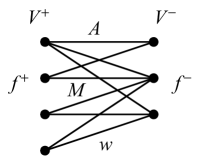
Figure 4: Valuated assignment problem

In applications the empty set often belongs to ${\rm dom\,}f^{+}$ (resp., ${\rm dom\,}f^{-}$), in which case ${\rm dom\,}f^{+}$ (resp., ${\rm dom\,}f^{-}$) forms the family of independent sets of a matroid. If $f^{+}\equiv 0$ and $f^{-}\equiv 0$ (with ${\rm dom\,}f^{+}=2^{V^{+}}$ and ${\rm dom\,}f^{-}=2^{V^{-}}$), this problem coincides with the conventional weighted matching problem.

An important special case of the M^♮-concave matching problem arises from a very special underlying graph $G_{\equiv}=(V^{+},V^{-};A_{\equiv})$ that represents a one-to-one correspondence between $V^{+}$ and $V^{-}$. In other words, given a pair of M^♮-concave set functions $f_{1},f_{2}:2^{V}\to\mathbb{R}\cup\{-\infty\}$ and a weight function $w:V\to\mathbb{R}$, let $V^{+}$ and $V^{-}$ be disjoint copies of $V$ and $A_{\equiv}=\{(v^{+},v^{-})\mid v\in V\}$, where $v^{+}\in V^{+}$ and $v^{-}\in V^{-}$ denote the copies of $v\in V$. The given functions $f_{1}$ and $f_{2}$ are regarded as set functions on $V^{+}$ and $V^{-}$, respectively. Then we obtain the following problem:

[M^♮-concave intersection problem] Given a pair of M^♮-concave set functions $f_{1},f_{2}:2^{V}\to\mathbb{R}\cup\{-\infty\}$ and a weight function $w:V\to\mathbb{R}$, find a subset $X$ that maximizes

$$w(X)+f_{1}(X)+f_{2}(X),$$ (11.3)

where $w(X)=\sum_{v\in X}w(v)$.

11.2 Optimality criterion by potentials

We show the optimality criterion for the M^♮-concave matching problem in terms of potentials, where a potential means a function $p:V^{+}\cup V^{-}\to\mathbb{R}$ (or a vector $p\in\mathbb{R}^{V^{+}\cup V^{-}}$) on the vertex set $V^{+}\cup V^{-}$. In the following theorem due to Murota (1996a) (see also Theorem 5.2.39 of Murota 2000a), the statement (1) refers to the existence of an appropriate potential, whereas its reformulation in (2) reveals the duality nature. For each arc $a=(u,v)\in A$, $\partial^{+}a$ denotes the initial (tail) vertex of $a$, and $\partial^{-}a$ the terminal (head) vertex of $a$, i.e., $\partial^{+}a=u\in V^{+}$ and $\partial^{-}a=v\in V^{-}$, where all the arcs are assumed to be directed from $V^{+}$ to $V^{-}$.

Theorem 11.1 (Potential criterion).

Let $M$ be a matching in $G=(V^{+},V^{-};A)$ satisfying (11.2) for the M^♮-concave matching problem to maximize (11.1).

(1) $M$ is an optimal matching if and only if there exists a potential $p:V^{+}\cup V^{-}\to\mathbb{R}$ such that

(i)  ${\displaystyle w(a)-p(\partial^{+}a)+p(\partial^{-}a)\ \left\{\begin{array}[]{ll}\leq 0&(a\in A),\\ =0&(a\in M),\end{array}\right.}$

(ii)  $\partial^{+}M$ is a maximizer of $f^{+}[+p^{+}]$,

(iii)  $\partial^{-}M$ is a maximizer of $f^{-}[-p^{-}]$,

where $p^{+}$ and $p^{-}$ are the restrictions of $p$ to $V^{+}$ and $V^{-}$, respectively, and $f^{+}[+p^{+}]$ and $f^{-}[-p^{-}]$ are defined by

$$f^{+}[+p^{+}](X) =f^{+}(X)+\sum\{p(u)\mid u\in X\}\qquad(X\subseteq V^{+}),$$

$$f^{-}[-p^{-}](Y) =f^{-}(Y)-\sum\{p(v)\mid v\in Y\}\qquad(Y\subseteq V^{-}).$$

(2)  ${\displaystyle\max_{M}\{w(M)+f^{+}(\partial^{+}M)+f^{-}(\partial^{-}M)\}}$

${\displaystyle=\min_{p}\{\max(f^{+}[+p^{+}])+\max(f^{-}[-p^{-}])\mid w(a)-p(\partial^{+}a)+p(\partial^{-}a)\leq 0\ (a\in A)\}.}$

(3) If $f^{+}$, $f^{-}$ and $w$ are all integer-valued, the potential $p$ in (1) and (2) can be chosen to be integer-valued.

(4) Let $p$ be a potential that satisfies (i)–(iii) in (1) for some (optimal) matching $M=M_{0}$. A matching $M^{\prime}$ is optimal if and only if it satisfies (i)–(iii) (with $M$ replaced by $M^{\prime}$).

In connection to (ii) and (iii) in (1) in Theorem 11.1, Theorem 3.4 shows:

$$X\in\arg\max(f^{+}[+p^{+}])$$

$$\iff\left\{\begin{array}[]{ll}f^{+}(X)-f^{+}(X-u+v)+p(u)-p(v)\geq 0&(\forall\,u\in X,\ \forall\,v\in V^{+}\setminus X),\\ f^{+}(X)-f^{+}(X-u)+p(u)\geq 0&(\forall\,u\in X),\\ f^{+}(X)-f^{+}(X+v)-p(v)\geq 0&(\forall\,v\in V^{+}\setminus X),\\ \end{array}\right.$$ (11.7)

$$Y\in\arg\max(f^{-}[-p^{-}])$$

$$\iff\left\{\begin{array}[]{ll}f^{-}(Y)-f^{-}(Y-u+v)-p(u)+p(v)\geq 0&(\forall\,u\in Y,\ \forall\,v\in V^{-}\setminus Y),\\ f^{-}(Y)-f^{-}(Y-u)-p(u)\geq 0&(\forall\,u\in Y),\\ f^{-}(Y)-f^{-}(Y+v)+p(v)\geq 0&(\forall\,v\in V^{-}\setminus Y).\\ \end{array}\right.$$ (11.11)

These expressions are crucial in deriving the second optimality criterion (Theorem 11.3) in Section 11.3 and in designing efficient algorithms for the M^♮-concave matching problem.

The optimality condition for the M^♮-concave intersection problem (11.3) deserves a separate statement in the form of weight splitting, though it is an immediate corollary of the above theorem.

Theorem 11.2 (Weight splitting for M^♮-concave intersection).

(1) A subset $X\subseteq V$ maximizes $w(X)+f_{1}(X)+f_{2}(X)$ if and only if there exist $w_{1},w_{2}:V\to\mathbb{R}$ such that

(i) [“weight splitting”]  $w(v)=w_{1}(v)+w_{2}(v)$   $(v\in V)$,

(ii)  $X$ is a maximizer of $f_{1}[+w_{1}]$,

(iii)  $X$ is a maximizer of $f_{2}[+w_{2}]$.

(2) ${\displaystyle\max_{X}\{w(X)+f_{1}(X)+f_{2}(X)\}}$

${\displaystyle=\min_{w_{1},w_{2}}\{\max(f_{1}[+w_{1}])+\max(f_{2}[+w_{2}])\mid w(v)=w_{1}(v)+w_{2}(v)\ (v\in V)\}.}$

(3) If $f_{1}$, $f_{2}$ and $w$ are all integer-valued, we may assume that $w_{1},w_{2}:V\to\mathbb{Z}$.

11.3 Optimality criterion by negative-cycles

As the second criterion for optimality we describe the negative-cycle criterion. First we need to introduce the auxiliary graph $G_{M}=(\tilde{V},A_{M})$ associated with a matching $M$ satisfying $\partial^{+}M\in{\rm dom\,}f^{+}$ and $\partial^{-}M\in{\rm dom\,}f^{-}$ in (11.2). Define $X=\partial^{+}M$ and $Y=\partial^{-}M$.

The vertex set $\tilde{V}$ of the auxiliary graph $G_{M}$ is given by $\tilde{V}=V^{+}\cup V^{-}\cup\{s^{+},s^{-}\}$, where $s^{+}$ and $s^{-}$ are new vertices often referred to as “source vertex” and “sink vertex” respectively. The arc set $A_{M}$ consists of nine disjoint parts:

$$A_{M}=(A^{\circ}\cup M^{\circ})\cup(A^{+}\cup F^{+}\cup S^{+})\cup(A^{-}\cup F^{-}\cup S^{-})\cup R,$$

where

$$A^{\circ} = \{a\mid a\in A\}\qquad\mbox{(copy of $A$)},$$

$$M^{\circ} = \{\overline{a}\mid a\in M\}\qquad\mbox{($\overline{a}$: reorientation of $a$)},$$

$$A^{+} = \{(u,v)\mid u\in X,\ v\in V^{+}\setminus X,\ X-u+v\in{\rm dom\,}f^{+}\},$$

$$F^{+} = \{(u,s^{+})\mid{u\in X,\ X-u\in{\rm dom\,}f^{+}\},}$$ (11.12)

$$S^{+} = \{(s^{+},v)\mid{v\in V^{+}\setminus X,\ X+v\in{\rm dom\,}f^{+}\},}$$

$$A^{-} = \{(v,u)\mid u\in Y,\ v\in V^{-}\setminus Y,\ Y-u+v\in{\rm dom\,}f^{-}\},$$

$$F^{-} = \{(s^{-},u)\mid{u\in Y,\ Y-u\in{\rm dom\,}f^{-}\},}$$

$$S^{-} = \{(v,s^{-})\mid{v\in V^{-}\setminus Y,\ Y+v\in{\rm dom\,}f^{-}\},}$$

$$R\ = {\{(s^{-},s^{+}),(s^{+},s^{-})\}.}$$

The arc length $\ell_{M}(a)$ for $a\in A_{M}$ is defined by

$$\ell_{M}(a)=\left\{\begin{array}[]{ll}-w(a)&(a\in A^{\circ}),\\ w(\overline{a})&(a=(u,v)\in M^{\circ},\ \overline{a}=(v,u)\in M),\\ f^{+}(X)-f^{+}(X-u+v)&(a=(u,v)\in A^{+}),\\ f^{+}(X)-f^{+}(X-u)&(a=(u,s^{+})\in F^{+}),\\ f^{+}(X)-f^{+}(X+v)&(a=(s^{+},v)\in S^{+}),\\ f^{-}(Y)-f^{-}(Y-u+v)&(a=(v,u)\in A^{-}),\\ f^{-}(Y)-f^{-}(Y-u)&(a=(s^{-},u)\in F^{-}),\\ f^{-}(Y)-f^{-}(Y+v)&(a=(v,s^{-})\in S^{-}),\\ 0&{(a\in R).}\end{array}\right.$$ (11.13)

A directed cycle in $G_{M}$ of a negative length with respect to the arc length $\ell_{M}$ is called a negative cycle. As is well known in network flow theory, there exists no negative cycle in $(G_{M},\ell_{M})$ if and only if there exists a potential $p:\tilde{V}\to\mathbb{R}$ such that

$$\ell_{M}(a)+p(\partial^{+}a)-p(\partial^{-}a)\geq 0\qquad(a\in A_{M}),$$ (11.14)

where $\partial^{+}a$ denotes the initial (tail) vertex of $a$, and $\partial^{-}a$ the terminal (head) vertex of $a$. With the use of (11.7), (11.11) and (11.14), Theorem 11.1 is translated into the following theorem; see Remark 11.1. This theorem (Murota 1996a, Theorem 5.2.42 of Murota 2003) gives an optimality criterion in terms of negative cycles.

Theorem 11.3 (Negative-cycle criterion).

In the M^♮-concave matching problem to maximize (11.1), a matching $M$ satisfying (11.2) is optimal if and only if there exists in the auxiliary graph $G_{M}$ no negative cycle with respect to the arc length $\ell_{M}$.

Remark 11.1.

The condition (11.14) for $a\in(F^{+}\cup S^{+})\cup(F^{-}\cup S^{-})$ refers to $p(s^{+})$ and $p(s^{-})$, while the potential $p$ in Theorem 11.1 is defined only on $V^{+}\cup V^{-}$. To derive (11.14) from Theorem 11.1 we may define $p(s^{+})=p(s^{-})=0$. Indeed, the conditions imposed on $p(s^{+})$ by (11.14) are

$$f^{+}(X)-f^{+}(X-u)+p(u)-p(s^{+})\geq 0\qquad(u\in X),$$

$$f^{+}(X)-f^{+}(X+v)+p(s^{+})-p(v)\geq 0\qquad(v\in V^{+}\setminus X),$$

which are satisfied by (11.7) if $p(s^{+})=0$. Similarly for $p(s^{-})$.  

11.4 Concluding remarks of section 11

Theorems 11.1 and 11.3 contain several standard results in matroid optimization, such as Frank’s weight splitting theorem (Frank 1981) for the weighted matroid intersection problem. The proofs of Theorems 11.1 and 11.3 can be found in Murota (1996a) and Section 5.2 of Murota (2000a). There are two key lemmas, called “upper-bound lemma” and “unique-max lemma,” which capture the essential properties inherent in M-concavity. On the basis of these optimality criteria efficient algorithms can be designed for the M^♮-concave matching problem. For algorithmic issues, see Murota (1996b) and Section 6.2 of Murota (2000a).

The valuated matching problem treated in this section is generalized to the submodular flow problem in Section 12.

12 Submodular Flow Problem

12.1 Submodular flow problem

Let $G=(V,A)$ be a directed graph with vertex set $V$ and arc set $A$. Suppose that each arc $a\in A$ is associated with upper-capacity $\overline{c}(a)$, lower-capacity $\underline{c}(a)$, and cost $\gamma(a)$ per unit flow. Furthermore, for each vertex $v\in V$, the amount of flow supply at $v$ is specified by $x(v)$.

The minimum cost flow problem is to find a flow $\xi=(\xi(a)\mid a\in A)$ that minimizes the total cost $\langle\gamma,\xi\rangle_{A}=\sum_{a\in A}\gamma(a)\xi(a)$ subject to the capacity constraint $\underline{c}(a)\leq\xi(a)\leq\overline{c}(a)$ $(a\in A)$ and the supply specification. Here the supply specification means a constraint that the boundary $\partial\xi$ of $\xi$ defined by

$$\partial\xi(v)=\sum\{\xi(a)\mid a\in\delta^{+}v\}-\sum\{\xi(a)\mid a\in\delta^{-}v\}\qquad(v\in V)$$ (12.1)

should be equal to a given value $x(v)$, where $\delta^{+}v$ and $\delta^{-}v$ denote the sets of arcs leaving (going out of) $v$ and entering (coming into) $v$, respectively. We can interpret $x(v)=\partial\xi(v)$ as the net amount of flow entering the network at $v$ from outside.

We consider the integer flow problem, which is described by an integer-valued upper-capacity $\overline{c}:A\to\mathbb{Z}\cup\{+\infty\}$, an integer-valued lower-capacity $\underline{c}:A\to\mathbb{Z}\cup\{-\infty\}$, a real-valued cost function $\gamma:A\to\mathbb{R}$, and an integer supply vector $x:V\to\mathbb{Z}$, where it is assumed that $\overline{c}(a)\geq\underline{c}(a)$ for each $a\in A$. The variable to be optimized is an integral flow $\xi:A\to\mathbb{Z}$.

[Minimum cost flow problem MCFP (linear arc cost)]

Minimize $$\Gamma_{0}(\xi)=\sum_{a\in A}\gamma(a)\xi(a)$$ (12.2)

subject to $$\underline{c}(a)\leq\xi(a)\leq\overline{c}(a)\qquad(a\in A),$$ (12.5)

$$\partial\xi=x,$$

$$\xi(a)\in\mathbb{Z}\qquad(a\in A).$$

A generalization of the minimum cost flow problem MCFP is obtained by relaxing the supply specification $\partial\xi=x$ to the constraint that the flow boundary $\partial\xi$ should belong to a given subset $B$ of $\mathbb{Z}^{V}$ representing “feasible” or “admissible” supplies:

$$\partial\xi\in B.$$ (12.6)

Such problem is called the submodular flow problem, if $B$ is an M-convex set (integral base polyhedron; see Remark 4.2). This problem is introduced by Edmonds and Giles (1977).

[Submodular flow problem MSFP₁ (linear arc cost)]

Minimize $$\Gamma_{1}(\xi)=\sum_{a\in A}\gamma(a)\xi(a)$$ (12.7)

subject to $$\underline{c}(a)\leq\xi(a)\leq\overline{c}(a)\qquad(a\in A),$$ (12.10)

$$\partial\xi\in B,$$

$$\xi(a)\in\mathbb{Z}\qquad(a\in A).$$

A further generalization of the problem is obtained by introducing a cost function for the flow boundary $\partial\xi$ rather than merely imposing the constraint $\partial\xi\in B$. Namely, with a function $f:\mathbb{Z}^{V}\to\mathbb{R}\cup\{+\infty\}$ we add a new term $f(\partial\xi)$ to the objective function, thereby imposing constraint $\partial\xi\in B={\rm dom\,}f$ implicitly. If the function $f$ is M-convex, the generalized problem is called the M-convex submodular flow problem, introduced by Murota (1999).

[M-convex submodular flow problem MSFP₂ (linear arc cost)]

Minimize $$\Gamma_{2}(\xi)=\sum_{a\in A}\gamma(a)\xi(a)+f(\partial\xi)$$ (12.11)

subject to $$\underline{c}(a)\leq\xi(a)\leq\overline{c}(a)\qquad(a\in A),$$ (12.14)

$$\partial\xi\in{\rm dom\,}f,$$

$$\xi(a)\in\mathbb{Z}\qquad(a\in A).$$

The special case of the M-convex submodular flow problem MSFP₂ with a $\{0,+\infty\}$-valued $f$ reduces to the submodular flow problem MSFP₁.

A still further generalization is possible by replacing the linear arc cost in $\Gamma_{2}$ with a separable convex function. Namely, using univariate convex functions $f_{a}:\mathbb{Z}\to\mathbb{R}\cup\{+\infty\}$ $(a\in A)$, we consider ${\displaystyle\sum_{a\in A}f_{a}(\xi(a))}$ instead of ${\displaystyle\sum_{a\in A}\gamma(a)\xi(a)}$ to obtain MSFP₃ below.

[M-convex submodular flow problem MSFP₃ (nonlinear arc cost)]

Minimize $$\Gamma_{3}(\xi)=\sum_{a\in A}f_{a}(\xi(a))+f(\partial\xi)$$ (12.15)

subject to $$\xi(a)\in{\rm dom\,}f_{a}\qquad(a\in A),$$ (12.18)

$$\partial\xi\in{\rm dom\,}f,$$

$$\xi(a)\in\mathbb{Z}\qquad(a\in A).$$

Obviously, MSFP₂ is a special case of MSFP₃ with

$$f_{a}(t)=\left\{\begin{array}[]{ll}\gamma(a)t&(t\in[\underline{c}(a),\overline{c}(a)]_{\mathbb{Z}}),\\ +\infty&(\mbox{otherwise}).\end{array}\right.$$ (12.19)

Conversely, MSFP₃ can be put into the form MSFP₂; see Remark 12.1.

Remark 12.1.

Problem MSFP₃ on $G=(V,A)$ can be written in the form of MSFP₂ on a larger graph $\tilde{G}=(\tilde{V},\tilde{A})$. We replace each arc $a=(u,v)\in A$ with a pair of arcs, $a^{+}=(u,v_{a}^{-})$ and $a^{-}=(v_{a}^{+},v)$, where $v_{a}^{+}$ and $v_{a}^{-}$ are newly introduced vertices. Accordingly, we have $\tilde{A}=\{a^{+},a^{-}\mid a\in A\}$ and $\tilde{V}=V\cup\{v_{a}^{+},v_{a}^{-}\mid a\in A\}$. For each $a\in A$ we consider a function $\tilde{f}_{a}:\mathbb{Z}^{2}\to\mathbb{R}\cup\{+\infty\}$ given by

$$\tilde{f}_{a}(t,s)=\left\{\begin{array}[]{ll}f_{a}(t)&(t+s=0),\\ +\infty&(\mbox{otherwise}),\end{array}\right.$$

and define $\tilde{f}:\mathbb{Z}^{\tilde{V}}\to\mathbb{R}\cup\{+\infty\}$ by

$$\tilde{f}(\tilde{x})=\sum_{a\in A}\tilde{f}_{a}(\tilde{x}(v_{a}^{+}),\tilde{x}(v_{a}^{-}))+f(\tilde{x}|_{V})\qquad(\tilde{x}\in\mathbb{Z}^{\tilde{V}}),$$

where $\tilde{x}|_{V}$ denotes the restriction of $\tilde{x}$ to $V$. For a flow $\tilde{\xi}:\tilde{A}\to\mathbb{Z}$, we have $\tilde{\xi}(a^{+})=\tilde{\xi}(a^{-})$ if $(\partial\tilde{\xi}(v_{a}^{+}),\partial\tilde{\xi}(v_{a}^{-}))\in{\rm dom\,}\tilde{f}_{a}$. Problem MSFP₃ is thus reduced to MSFP₂ with objective function $\tilde{\Gamma}_{2}(\tilde{\xi})=\tilde{f}(\partial\tilde{\xi})$, where the function $\tilde{f}$ is M-convex.  

Remark 12.2.

The M^♮-concave intersection problem (Section 9.1) can be formulated as an M-convex submodular flow problem. Suppose we want to maximize the sum $f_{1}(x)+f_{2}(x)$ of two M^♮-concave functions $f_{1},f_{2}:\mathbb{Z}^{n}\to\mathbb{R}\cup\{-\infty\}$. Let $\tilde{f}_{1},\tilde{f}_{2}:\mathbb{Z}^{n+1}\to\mathbb{R}\cup\{-\infty\}$ be the associated M-concave functions; see (4.18). We consider an M-convex submodular flow problem on the bipartite graph $G=(V_{1}\cup V_{2},A)$ in Fig. 5, where $V_{i}=\{v_{i0},v_{i1},\ldots,v_{in}\}$ for $i=1,2$ and $A=\{(v_{1j},v_{2j})\mid j=0,1,\ldots,n\}$. The boundary cost function $f:\mathbb{Z}^{V_{1}}\times\mathbb{Z}^{V_{2}}\to\mathbb{R}\cup\{+\infty\}$ is defined by $f(x_{1},x_{2})=-\tilde{f}_{1}(x_{1})-\tilde{f}_{2}(-x_{2})$ for $x_{1}\in\mathbb{Z}^{V_{1}}$ and $x_{2}\in\mathbb{Z}^{V_{2}}$, which is an M-convex function. The arc costs are identically zero and no capacity constraints are imposed ($\gamma(a)=0$, $\overline{c}(a)=+\infty$, $\underline{c}(a)=-\infty$ for all $a\in A$). Since $x_{1}=-x_{2}$ if $(x_{1},x_{2})=\partial\xi$ for a flow $\xi$ in this network, this M-convex submodular flow problem is equivalent to the problem of maximizing $f_{1}(x)+f_{2}(x)$. Theorem 9.4 for the M-convex intersection problem can be regarded as a special case of Theorem 12.1 for the M-convex submodular flow problem.  

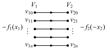
Figure 5: M-convex submodular flow problem for M^♮-concave intersection problem

In subsequent sections we show optimality criteria for the M-convex submodular flow problem in terms of potentials and negative cycles.

12.2 Optimality criterion by potentials

We show the optimality criterion for the M-convex submodular flow problem MSFP₃ in terms of potentials. A potential means a function $p:V\to\mathbb{R}$ (or a vector $p\in\mathbb{R}^{V}$) on the vertex set $V$. The coboundary of a potential $p$ is a function $\delta p:A\to\mathbb{R}$ on the arc set $A$ defined by

$$\delta p(a)=p(\partial^{+}a)-p(\partial^{-}a)\qquad(a\in A),$$ (12.20)

where, for each arc $a\in A$, $\partial^{+}a$ denotes the initial (tail) vertex of $a$ and, $\partial^{-}a$ the terminal (head) vertex of $a$. The following theorem is due to Murota (1999); see also Section 9.4 of Murota (2003).

Theorem 12.1 (Potential criterion).

Consider the M-convex submodular flow problem MSFP₃.

(1) For a feasible flow $\xi:A\to\mathbb{Z}$, two conditions (OPT) and (POT) below are equivalent.

(OPT) $\xi$ is an optimal flow.

(POT) There exists a potential $p:V\to\mathbb{R}$ such that

(i)  $\xi(a)\in\arg\min f_{a}[+\delta p(a)]$   for every $a\in A$,   and

(ii)  $\partial\xi\in\arg\min f[-p]$.

(2) Suppose that a potential $p:V\to\mathbb{R}$ satisfies (i) and (ii) above for an optimal flow $\xi$. A feasible flow $\xi^{\prime}$ is optimal if and only if

(i)  $\xi^{\prime}(a)\in\arg\min f_{a}[+\delta p(a)]$   for every $a\in A$,   and

(ii)  $\partial\xi^{\prime}\in\arg\min f[-p]$.

(3) If the cost functions $f_{a}$ $(a\in A)$ and $f$ are integer-valued, there exists an integer-valued potential $p:V\to\mathbb{Z}$ in (POT). Moreover, the set of integer-valued optimal potentials,

$$\Pi^{*}=\{p\mid p:\mbox{integer-valued optimal potential\,}\},$$

is an L-convex set .

In connection to (i) and (ii) in (POT) in Theorem 12.1, note the equivalences:

$$\xi(a)\in\arg\min f_{a}[+\delta p(a)]$$

$$\iff f_{a}(\xi(a)+d)-f_{a}(\xi(a))+d[p(\partial^{+}a)-p(\partial^{-}a)]\geq 0\qquad(d=\pm 1),$$ (12.21)

$$\partial\xi\in\arg\min f[-p]$$

$$\iff\Delta f(\partial\xi;v,u)+p(u)-p(v)\geq 0\qquad(\forall u,v\in V),$$ (12.22)

where

$$\Delta f(z;v,u)=f(z+\chi_{v}-\chi_{u})-f(z)\qquad(z\in{\rm dom\,}f;u,v\in V).$$ (12.23)

These expressions are crucial in deriving the second optimality criterion (Theorem 12.2) in Section 12.3 and in designing efficient algorithms for the M-convex submodular flow problem.

12.3 Optimality criterion by negative cycles

The optimality of an M-convex submodular flow can also be characterized by the nonexistence of negative cycles in an auxiliary network. This fact leads to the cycle-cancelling algorithm. We consider the M-convex submodular flow problem MSFP₂ that has a linear arc cost. This is not restrictive, since MSFP₃ can be put in the form of MSFP₂ (Remark 12.1).

For a feasible flow $\xi:A\to\mathbb{Z}$ we define an auxiliary network as follows. Let $G_{\xi}=(V,A_{\xi})$ be a directed graph with vertex set $V$ and arc set $A_{\xi}=A_{\xi}^{\circ}\cup B_{\xi}^{\circ}\cup C_{\xi}$ consisting of three disjoint parts:

$$A_{\xi}^{\circ} = \{a\mid a\in A,\ \xi(a)<\overline{c}(a)\},$$

$$B_{\xi}^{\circ} = \{\overline{a}\mid a\in A,\ \underline{c}(a)<\xi(a)\}\qquad\mbox{($\overline{a}$: reorientation of $a$)},$$

$$C_{\xi} = \{(u,v)\mid u,v\in V,\ u\not=v,\ \partial\xi-(\chi_{u}-\chi_{v})\in{\rm dom\,}f\}.$$ (12.24)

We define an arc length function $\ell_{\xi}:A_{\xi}\to\mathbb{R}$ by

$$\ell_{\xi}(a)=\left\{\begin{array}[]{ll}\gamma(a)&(a\in A_{\xi}^{\circ}),\\ -\gamma(\overline{a})&(a\in B_{\xi}^{\circ},\ \overline{a}\in A),\\ \Delta f(\partial\xi;v,u)&(a=(u,v)\in C_{\xi}).\\ \end{array}\right.$$ (12.25)

We refer to $(G_{\xi},\ell_{\xi})$ as the auxiliary network.

A directed cycle in $G_{\xi}$ of a negative length with respect to the arc length $\ell_{\xi}$ is called a negative cycle. As is well known in network flow theory, there exists no negative cycle in $(G_{\xi},\ell_{\xi})$ if and only if there exists a potential $p:V\to\mathbb{R}$ such that

$$\ell_{\xi}(a)+p(\partial^{+}a)-p(\partial^{-}a)\geq 0\qquad(a\in A_{\xi}).$$ (12.26)

With the use of (12.21), (12.22) and (12.26), Theorem 12.1 is translated into the following theorem (Murota 1999; see also Section 9.5 of Murota 2003), which gives an optimality criterion in terms of negative cycles.

Theorem 12.2 (Negative-cycle criterion).

For a feasible flow $\xi:A\to\mathbb{Z}$ to the M-convex submodular flow problem MSFP₂, the conditions (OPT) and (NNC) below are equivalent.

(OPT) $\xi$ is an optimal flow.

(NNC) There exists no negative cycle in the auxiliary network $(G_{\xi},\ell_{\xi})$ with $\ell_{\xi}$ of (12.25).

Cycle cancellation:

The negative-cycle optimality criterion states that the existence of a negative cycle implies the non-optimality of a feasible flow. This suggests the possibility of improving a non-optimal feasible flow by the cancellation of a suitably chosen negative cycle.

Suppose that negative cycles exist in the auxiliary network $(G_{\xi},\ell_{\xi})$ for a feasible flow $\xi$, where the arc length $\ell_{\xi}$ is defined by (12.25). Choose a negative cycle having the smallest number of arcs, and let $Q$ $(\subseteq A_{\xi})$ be the set of its arcs. Modifying the flow $\xi$ along $Q$ by a unit amount we obtain a new flow $\overline{\xi}$ defined by

$$\overline{\xi}(a)=\left\{\begin{array}[]{ll}\xi(a)+1&(a\in Q\cap A_{\xi}^{\circ}),\\ \xi(a)-1&(\overline{a}\in Q\cap B_{\xi}^{\circ}),\\ \xi(a)&\mbox{(otherwise)}.\end{array}\right.$$ (12.27)

The following theorem shows that the updated flow $\overline{\xi}$ is a feasible flow with an improvement in the objective function in (12.11):

$$\Gamma_{2}(\xi)=\sum_{a\in A}\gamma(a)\xi(a)+f(\partial\xi).$$

Theorem 12.3.

For a feasible flow $\xi:A\to\mathbb{Z}$ to the M-convex submodular flow problem MSFP₂, let $Q$ be a negative cycle having the smallest number of arcs in $(G_{\xi},\ell_{\xi})$. Then $\overline{\xi}$ in (12.27) is a feasible flow and

$$\Gamma_{2}(\overline{\xi})\leq\Gamma_{2}(\xi)+\ell_{\xi}(Q)<\Gamma_{2}(\xi).$$ (12.28)

12.4 Concluding remarks of section 12

On the basis of the optimality criteria in Theorems 12.1 and 12.2 we can design efficient algorithms for the M-convex submodular flow problem, where the expressions (12.21) and (12.22) are crucial. For algorithmic issues, see Murota (1999), Section 10.4 of Murota (2003), Iwata and Shigeno (2003), Murota and Tamura (2003b), and Iwata et al. (2005).

13 Discrete Fixed Point Theorem

Discrete fixed point theorems in discrete convex analysis originate in the theorem of Iimura et al. (2005) based on Iimura (2003), which is described in this section. Subsequent development and other types of discrete fixed point theorems are mentioned in Section 13.5.

13.1 Discrete fixed point theorem

To motivate the discrete fixed point theorem of Iimura et al. (2005), we first take a glimpse at Kakutani’s fixed point theorem.

Let $S$ be a subset of $\mathbb{R}^{n}$ and $F$ be a set-valued mapping (correspondence) from $S$ to itself, which is denoted as $F:S\to\to S$ (or $F:S\to 2^{S}$). A point $x\in S$ satisfying $x\in F(x)$ is said to be a fixed point of $F$. Kakutani’s fixed point theorem reads as follows.

Theorem 13.1.

A set-valued mapping $F:S\to\to S$, where $S\subseteq\mathbb{R}^{n}$, has a fixed point if

(a) $S$ is a bounded closed convex subset of $\mathbb{R}^{n}$,

(b) For each $x\in S$, $F(x)$ is a nonempty closed convex set, and

(c) $F$ is upper-hemicontinuous.

In the discrete fixed point theorem (Theorem 13.2 below) we are concerned with $F:S\to\to S$, where $S$ is a subset of $\mathbb{Z}^{n}$. The three conditions (a) to (c) in Theorem 13.1 above are “discretized” as follows.

• Condition (a) assumes that the domain of definition $S$ is nicely-shaped or well-behaved. In the discrete case we assume $S$ to be “integrally convex.”

• Condition (b) assumes that each value $F(x)$ is nicely-shaped or well-behaved. In the discrete case we assume that $F(x)=\overline{F(x)}\cap\mathbb{Z}^{n}$, where $\overline{F(x)}$ denotes the convex hull of $F(x)$.

• Condition (c) assumes that mapping $F$ is continuous in some appropriate sense. In the discrete case we assume $F$ to be “direction-preserving.”

The key concepts, “integrally convex set” and “direction-preserving mapping,” are explained in Section 13.2. The discrete fixed point theorem of Iimura et al. (2005) is the following.

Theorem 13.2.

A set-valued mapping $F:S\to\to S$, where $S\subseteq\mathbb{Z}^{n}$, has a fixed point if

(a) $S$ is a nonempty finite integrally convex subset of $\mathbb{Z}^{n}$,

(b) For each $x\in S$, $F(x)$ is nonempty and $F(x)=\overline{F(x)}\cap\mathbb{Z}^{n}$, and

(c) $F$ is direction-preserving.

13.2 Integrally convex set and direction-preserving mapping

Integrally convex set:

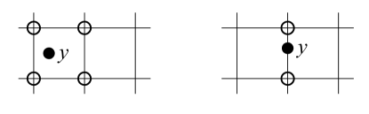
Figure 6: Integral neighbor $N(y)$ of $y$   ($\circ$: point of $N(y)$)

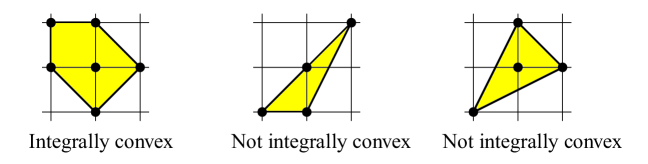
Figure 7: Concept of integrally convex sets

The integral neighborhood of a point $y\in\mathbb{R}^{n}$ is defined as

$$N(y)=\{z\in\mathbb{Z}^{n}\mid\|z-y\|_{\infty}<1\}.$$ (13.1)

See Fig. 6. A set $S\subseteq\mathbb{Z}^{n}$ is said to be integrally convex if

$$y\in\overline{S}\ \Longrightarrow y\in\overline{S\cap N(y)}$$ (13.2)

for any $y\in\mathbb{R}^{n}$ (Favati and Tardella 1990). Figure 7 illustrates this concept. We have $S=\overline{S}\cap\mathbb{Z}^{n}$ for an integrally convex set $S$. It is known that L^♮-convex sets and M^♮-convex sets are integrally convex. See Section 3.4 of Murota (2003) and Moriguchi et al. (2016) for more about integral convexity.

Direction-preserving mapping:

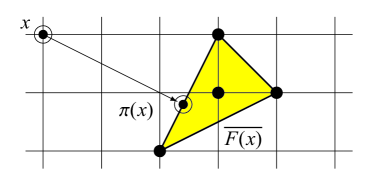
Figure 8: Projection $\pi(x)$ with $\sigma(x)={\rm sign\,}(\pi(x)-x)=(+1,-1)$

Let $S$ be a subset of $\mathbb{Z}^{n}$ and $F:S\to\to S$ be a set-valued mapping (correspondence) from $S$ to $S$. For $x=(x_{1},\ldots,x_{n})\in\mathbb{Z}^{n}$ we denote by $\pi(x)=(\pi_{1}(x),\ldots,\pi_{n}(x))\in\mathbb{R}^{n}$ the projection of $x$ to $\overline{F(x)}$; see Fig. 8. This means that $\pi(x)$ is the point of $\overline{F(x)}$ that is nearest to $x$ with respect to the Euclidean norm. We define the direction sign vector $\sigma(x)\in\{+1,0,-1\}^{n}$ as

$$\sigma(x)=(\sigma_{1}(x),\ldots,\sigma_{n}(x))=({\rm sign\,}(\pi_{1}(x)-x_{1}),\ldots,{\rm sign\,}(\pi_{n}(x)-x_{n})),$$

where

$${\rm sign\,}(y)=\left\{\begin{array}[]{rl}+1&(y>0),\\ 0&(y=0),\\ -1&(y<0).\\ \end{array}\right.$$

Then we say that $F$ is direction-preserving if for all $x,z\in S$ with $\|x-z\|_{\infty}\leq 1$ it holds that

$$\sigma_{i}(x)>0\ \Longrightarrow\ \sigma_{i}(z)\geq 0\qquad(i=1,\ldots,n).$$ (13.3)

Note that this is equivalent to saying that $\sigma_{i}(x)\sigma_{i}(z)\not=-1$ for each $i=1,\ldots,n$ if $x,z\in S$ and $\|x-z\|_{\infty}\leq 1$. Being direction-preserving is interpreted as being “continuous” in the discrete setting.

13.3 Illustrative examples

Example 13.1.

The significance of being direction-preserving is most transparent in the case of $n=1$. Let $S=[a,b]_{\mathbb{Z}}$ be an integer interval with $a,b\in\mathbb{Z}$ and $a\leq b$. Consider $F:S\to\to S$ represented as $F(x)=[\alpha(x),\beta(x)]_{\mathbb{Z}}$, where $\alpha(x),\beta(x)\in\mathbb{Z}$ and $a\leq\alpha(x)\leq\beta(x)\leq b$. The projection $\pi(x)$ and the direction sign vector $\sigma(x)$ are given by

$$\pi(x)=\left\{\begin{array}[]{ll}x&(\alpha(x)\leq x\leq\beta(x)),\\ \alpha(x)&(x\leq\alpha(x)-1),\\ \beta(x)&(x\geq\beta(x)+1),\\ \end{array}\right.\quad\sigma(x)=\left\{\begin{array}[]{ll}0&(\alpha(x)\leq x\leq\beta(x)),\\ +1&(x\leq\alpha(x)-1),\\ -1&(x\geq\beta(x)+1).\\ \end{array}\right.$$

Suppose that $F$ is direction-preserving, which means $\sigma(x)\sigma(x+1)\not=-1$ for all $x$ with $a\leq x<b$. There are three possibilities:

(i) $\sigma(x)=+1$ for all $x\in S$,

(ii) $\sigma(x)=-1$ for all $x\in S$,

(iii) $\sigma(x)=0$ for some $x\in S$.

In the first case (i) we must have $x+1\leq\alpha(x)\leq b$ for all $x\in S$, but this is impossible for $x=b$. Similarly, the second case (ii) is not possible, either. Therefore, we must have the third case (iii), and then the $x$ satisfying $\sigma(x)=0$ is a fixed point of $F$.  

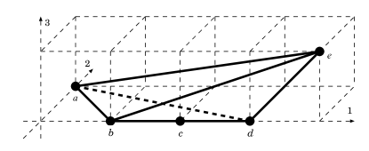
Figure 9: Necessity of the assumption of integral convexity

Example 13.2.

The assumption (a) of integral convexity in Theorem 13.2 cannot be weakened to the “hole-free” property: $S=\overline{S}\cap\mathbb{Z}^{n}$. Let $n=3$ and consider a subset $S$ of $\mathbb{Z}^{3}$ (Fig. 9) given by

$$S=\{a=(0,1,0),\ b=(1,0,0),\ c=(2,0,0),\ d=(3,0,0),\ e=(4,0,1)\},$$

which is not integrally convex, but satisfies $S=\overline{S}\cap\mathbb{Z}^{n}$. Define $F:S\to\to S$ by

$$F(a)=F(b)=\{e\},\quad F(c)=\{a,e\},\quad F(d)=F(e)=\{a\}.$$

For each $x\in S$, $F(x)$ is a nonempty subset of $S$ satisfying $F(x)=\overline{F(x)}\cap\mathbb{Z}^{n}$. Furthermore, $F$ is direction-preserving. Indeed we have

$$\begin{array}[]{lcl@{}rrr@{}l}\pi(a)-a&=&(&4,&-1,&1&),\\ \pi(b)-b&=&(&3,&0,&1&),\\ \pi(c)-c&=&(&0,&1/2,&1/2&),\\ \pi(d)-d&=&(&-3,&1,&0&),\\ \pi(e)-e&=&(&-4,&1,&-1&),\end{array}\quad\begin{array}[]{lcl@{}rrr@{}l}\sigma(a)&=&(&+1,&-1,&+1&),\\ \sigma(b)&=&(&+1,&0,&+1&),\\ \sigma(c)&=&(&0,&+1,&+1&),\\ \sigma(d)&=&(&-1,&+1,&0&),\\ \sigma(e)&=&(&-1,&+1,&-1&)\end{array}$$

and the condition (13.3) holds for every pair $(x,z)$ with $\|x-z\|_{\infty}\leq 1$, i.e., for $(x,z)=(a,b),(b,c),(c,d),(d,e)$. Thus, $F$ meets the conditions (b) and (c) in Theorem 13.2, but $F$ has no fixed point.  

13.4 Proof outline

The proof of Theorem 13.2 consists of the following three major steps; the reader is referred to Iimura et al. (2005) for the detail.

1. An integrally convex set $S$ has a simplicial decomposition $\mathcal{T}$ with a nice property. For each $y\in\mathbb{R}^{n}$ contained in the convex hull of $S$, let $T(y)$ denote the smallest simplex in $\mathcal{T}$ that contains $y$. Then the simplicial decomposition $\mathcal{T}$ has the property that all the vertices of $T(y)$ belong to the integral neighborhood $N(y)$ of $y$. That is, the set of the vertices of $T(y)$, to be denoted by $V(y)$, is given as $V(y)=T(y)\cap N(y)$.

2. With reference to the simplicial decomposition $\mathcal{T}$, we define a piecewise linear extension, say, $f$ of the projection $\pi$ by

   $$f(y)=\sum_{x\in V(y)}\lambda_{x}\pi(x)\qquad(y=\sum_{x\in V(y)}\lambda_{x}x,\ \ \sum_{x\in V(y)}\lambda_{x}=1,\quad\lambda_{x}\geq 0).$$

   By Brouwer’s fixed point theorem applied to $f:\overline{S}\to\overline{S}$, we obtain a fixed point $y^{*}\in\overline{S}$ of $f$, i.e., $y^{*}=f(y^{*})$.

3. From the equations

   $$\sum_{x\in V(y^{*})}\lambda_{x}(\pi(x)-x)=\sum_{x\in V(y^{*})}\lambda_{x}\pi(x)-\sum_{x\in V(y^{*})}\lambda_{x}x=f(y^{*})-y^{*}={\bf 0}$$

   and the assumption of $F$ being direction-preserving, we see that $\pi(x)-x={\bf 0}$ for some $x\in V(y^{*})$. Let $x^{*}$ be such a point in $V(y^{*})$. Then $x^{*}$ is a fixed point of $F$, since $x^{*}=\pi(x^{*})\in\overline{F(x^{*})}$, from which follows $x^{*}\in\overline{F(x^{*})}\cap\mathbb{Z}^{n}=F(x^{*})$ by condition (b).

13.5 Concluding remarks of section 13

The discrete fixed point theorem initiated by Iimura (2003) and Iimura et al. (2005) aims at a discrete version of Brouwer’s fixed point theorem. Related work in this direction includes van der Laan et al. (2006), Danilov and Koshevoi (2007), Chen and Deng (2006, 2008, 2009), Yang (2008, 2009), Talman and Yang (2009), Iimura and Yang (2009), Iimura (2010), Deng et al. (2011), van der Laan et al. (2011), and Iimura et al. (2012). Discrete fixed point theorems are used successfully in showing the existence of a competitive equilibrium under indivisibility, a pure Nash equilibrium with discrete strategy sets, etc.

Efforts are made to weaken the condition (c) of “direction preserving” in Theorem 13.2. Weaker conditions called “locally gross direction preserving” and “simplicially locally gross direction preserving” are considered by Yang (2008, 2009), Iimura and Yang (2009), Iimura (2010). Further variants are found in Talman and Yang (2009), van der Laan et al. (2011), and Iimura et al. (2012). These studies, however, share the framework of mappings and correspondences defined on integrally convex sets or their simplicial divisions.

The proof of Theorem 13.2 by Iimura et al. (2005) is not constructive, relying on Brouwer’s fixed point theorem. Constructive proofs are given by van der Laan et al. (2006) and van der Laan et al. (2011). Computational complexity of finding a fixed point for direction-preserving mappings is discussed by Chen and Deng (2006, 2008, 2009) and Deng et al. (2011).

Another type of (discrete) fixed point theorem, the lattice-theoretical fixed point theorem of Tarski (1955), is a powerful tool used extensively in economics and game theory; see Milgrom and Roberts (1990), Vives (1990), and Topkis (1998). For stable matchings, use and power of Tarski’s fixed point theorem are demonstrated by Adachi (2000), Fleiner (2003), and Farooq et al. (2012). It may be said, however, that Tarski’s fixed point theorem is rather independent of discrete convex analysis.

Yet another type of discrete fixed point theorems are considered in the literature, including Robert (1986), Shih and Dong (2005), Richard (2008), Sato and Kawasaki (2009) and Kawasaki et al. (2013).

14 Other Topics

14.1 Matching market and economy with indivisible goods

Since the seminal paper by Kelso and Crawford (1982), the concept of gross substitutes with its variants has turned out to be pivotal in discussing matching market and economy with indivisible goods. The literature includes, e.g., Roth and Sotomayor (1990), Bikhchandani and Mamer (1997), Gul and Stacchetti (1999), Ausubel and Milgrom (2002), Milgrom (2004), Hatfield and Milgrom (2005), Ausubel (2006), Sun and Yang (2006), Milgrom and Strulovici (2009), and Hatfield et al. (2016).

Application of discrete convex analysis to economics was started by Danilov et al. (1998, 2001) for the Walrasian equilibrium of indivisible markets (see also Chapter 11 of Murota 2003). The interaction between economics and discrete convex analysis was reinforced decisively by the observation of Fujishige and Yang (2003) that M^♮-concavity (of set functions) is equivalent to the gross substitutes property (Theorem 3.7 in Section 3.3). This equivalence is extended to functions in integer variables (Section 4.3). While the reader is referred to Tamura (2004) and Chapter 11 of Murota (2003) for this earlier development, we mention more recent papers below.

As described in Section 10, the Fujishige-Tamura model of two-sided matching markets, proposed by Fujishige and Tamura (2006, 2007), is a common generalization of the stable marriage model (Gale and Shapley 1962) and the assignment game (Shapley and Shubik 1972).

Inoue (2008) uses the property of M^♮-convex sets that they are closed under (Minkowski) summation, to show that the weak core in a finite exchange economy is nonempty if every agent’s upper contour set is M^♮-convex. Kojima et al. (2018) present a unified treatment of two-sided matching markets with a variety of distributional constraints that can be represented by M^♮-concave functions. It is shown that the generalized deferred acceptance algorithm is strategy-proof and yields a stable matching. Yokote (2016) considers a market in which each buyer demands at most one unit of commodity and each seller produces multiple units of several types of commodities. The core and the competitive equilibria are shown to exist and coincide under the assumption that the cost function of each seller is M^♮-convex.

Algorithmic aspects of Walrasian equilibria are fully investigated by Paes Leme and Wong (2020) in a general setting, in which the algorithms from discrete convex analysis are singled out as efficient methods for the gross substitutes case. See also Paes Leme (2017) as well as Murota and Tamura (2003b) and Section 11.5 of Murota (2003).

14.2 Trading networks

M^♮-concavity plays a substantial role in the modeling and analysis of vertical trading networks (supply chain networks) introduced by Ostrovsky (2008) and investigated in a more general setting by Hatfield et al. (2013), Fleiner (2014), Fleiner et al. (2015), Ikebe et al. (2015), Ikebe and Tamura (2015), and Candogan et al. (2016).

In a trading network, an agent is identified with a vertex (node) of the network. In-coming arcs to a vertex represent the trades in which the agent acts as a buyer and out-going arcs represent the trades in which the agent acts as a seller. Each vertex $v$ of the network is associated with a choice function $C_{v}$ and/or a valuation function $f_{v}$ of the agent, defined on the set $U_{v}\cup W_{v}$ of the arcs incident to $v$, where $U_{v}$ is the set of in-coming arcs to the vertex $v$ and $W_{v}$ is the set of out-going arcs from $v$. In particular, the function $f_{v}$ is a set function on $U_{v}\cup W_{v}$ in the single-unit case, whereas it is a function on $\mathbb{Z}^{U_{v}\cup W_{v}}$ in the multi-unit case.

In the single-unit case, Ostrovsky (2008) identifies the key property of a choice function, called the same-side substitutability (SSS) and the cross-side complementarity (CSC), which are discussed in Section 3.5. These properties are satisfied by the choice function induced from a unique-selecting twisted M^♮-concave valuation function $f_{v}$, with twisting by $W_{v}$; see Theorem 3.13. The multi-unit case is treated by Ikebe and Tamura (2015). The conditions (SSS) and (CSC) are generalized to (SSS-CSC¹[$\mathbb{Z}$]) and (SSS-CSC²[$\mathbb{Z}$]), and these conditions are shown to be satisfied by the choice function induced from a unique-selecting twisted M^♮-concave valuation $f_{v}$; see Theorem 4.14 in Section 4.5.

Discrete convex analysis is especially relevant and useful when valuation functions and the price vector $p$ are explicitly involved in the model as in Hatfield et al. (2013), Ikebe et al. (2015), and Candogan et al. (2016). Specifically, we can use the results from discrete convex analysis as follows:

• The existence of a competitive equilibrium (Hatfield et al. 2013, Definition 3) can be proved with the aid of the M^♮-concave intersection theorem (Theorem 9.4).

• The lattice structure of the equilibrium price vectors can be shown through the conjugacy relationship between M^♮-concavity and L^♮-convexity (Section 7.2).

• The equivalence of chain stability and stability can be established with the aid of the negative-cycle criterion for the M-convex submodular flow problem (Theorem 12.2). Recall from Remark 12.2 that the M^♮-concave intersection problem can be formulated as an M-convex submodular flow problem.

• Fundamental computational problems for a trading network, such as checking stability, computing a competitive equilibrium, and maximizing the welfare, can often be solved with the aid of algorithms known in discrete convex analysis, such as those for maximizing M^♮-concave functions and for solving the M-convex submodular flow problem. See Candogan et al. (2016) as well as Murota and Tamura (2003b), Section 11.5 of Murota (2003), and Ikebe et al. (2015).

14.3 Congestion games

Congestion games (Rosenthal 1973), which are equivalent to (exact) “finite” potential games (Monderer and Shapley 1996), are a class of games possessing a Nash equilibrium in pure strategies. There are various generalizations of potential games, such as: ordinal and generalized ordinal (Monderer and Shapley 1996) and best-response (Voorneveld 2000) potential games. For algorithmic aspects of congestion games, we refer to Roughgarden (2007) and Tardos and Wexler (2007).

Recently, a connection is made by Fujishige et al. (2015) between congestion games on networks and discrete convex analysis. It has been known (Fotakis 2010) that for every congestion game on an extension-parallel network, considered by Holzman and Law-yone (2003), any best-response sequence reaches a pure Nash equilibrium of the game in $n$ steps, where $n$ is the number of players. It is pointed out by Fujishige et al. (2015) that the fast convergence of best-response sequences is a consequence of M^♮-convexity of the associated potential function, which is a laminar convex function and hence is M^♮-convex; see (4.35) in Section 4.6.

In economics, potential games on some subset of a Euclidean space are more widely studied. A maximizer of (some sort of) potential function is a Nash equilibrium. We also have the converse if the potential function is “concave,” since local optimality implies the global optimality there. Ui (2006, 2008) studies the condition for a local maximizer of a function on the integer lattice to become a global maximizer of the function as well, with application to best-response potential games on the integer lattice. In Ui (2008), it is shown that a condition analogous to midpoint concavity, called “larger midpoint property,” is sufficient for the equivalence of local optimality and global optimality, and shows the equivalence of a Nash equilibrium and a maximizer of the best-response potential function. A more general condition for the equivalence of local and global optimality is studied in Ui (2006), along with its relation to M-, L-, L^♮-, and M^♮-convex functions.

14.4 Integrally concave games

Another study on the games on the integer lattice $\mathbb{Z}^{n}$ is found in Iimura and Watanabe (2014), which deals with $n$-person symmetric games with integrally concave payoff functions defined on the $n$-product of a finite integer interval. Here, the integral concavity is in the sense of Favati and Tardella (1990); see also Section 3.4 of Murota (2003). It is shown that every game in this class of games has a (not necessarily symmetric) Nash equilibrium, which is located within a unit distance from the diagonal of strategy space. Although assuming concavity on the entire strategy space is somewhat stringent, this result generalizes the result of Cheng et al. (2004) that every $n$-person symmetric “two-strategy” game has a (not necessarily symmetric) Nash equilibrium, because any real-valued function on the $n$-product of a doubleton is integrally concave. A further generalization has been made by Iimura and Watanabe (2016), which implies the existence of an equilibrium in discrete Cournot game with concave industry revenue, convex cost, and nonincreasing inverse demand.

14.5 Unimodularity and tropical geometry

Unimodular coordinate transformations are a natural operation for discrete convexity. In Section 4.7 we have mentioned that a function $f$ is twisted M^♮-concave if and only if it is represented as $f(x)=g(Ux)$ with $U={\rm diag}(1,\ldots,1,-1,\ldots,-1)$ for some M^♮-concave function $g$. Another such example is multimodular functions of Hajek (1985) used in discrete-event control (Altman et al. 2000). A function $f:\mathbb{Z}^{n}\to\mathbb{R}\cup\{+\infty\}$ is said to be multimodular if the function $\tilde{f}:\mathbb{Z}^{n+1}\to\mathbb{R}\cup\{+\infty\}$ defined by $\tilde{f}(x_{0},x)=f(x_{1}-x_{0},x_{2}-x_{1},\ldots,x_{n}-x_{n-1})$ for $x_{0}\in\mathbb{Z}$ and $x\in\mathbb{Z}^{n}$ is submodular in $n+1$ variables. This means that $f$ is multimodular if and only if the function $g(x)=f(Dx)$ is L^♮-convex, where $D=(d_{ij}\mid 1\leq i,j\leq n)$ is a bidiagonal matrix defined by $d_{ii}=1\ (i=1,\ldots,n)$ and $d_{i+1,i}=-1\ (i=1,\ldots,n-1)$. This matrix $D$ is unimodular, and its inverse $D^{-1}$ is an integral matrix with $(D^{-1})_{ij}=1$ for $i\geq j$ and $(D^{-1})_{ij}=0$ for $i<j$. Therefore, a function $f$ is multimodular if and only if it is represented as $f(x)=g(Ux)$ with $U=D^{-1}$ for some L^♮-convex function $g$.

The fundamental role of unimodularity for discrete convexity, beyond unimodular coordinate transformations, is investigated in Danilov and Koshevoy (2004) under the name of “unimodular systems.” An application of unimodular systems to competitive equilibrium is found in Danilov et al. (2001).

Another recent topic, of a similar flavor, is tropical geometry. Baldwin and Klemperer (2019) investigate indivisibility issues in terms of tropical geometry. The Ricardian theory of international trade is treated by Shiozawa (2015), mechanism design by Crowell and Tran (2016), and dominant strategy implementation by Weymark (2016). The interaction of tropical geometry with economics has just begun.

Acknowledgements

The author would like to thank Zaifu Yang for offering the opportunity of this survey paper. Special thanks go to Akiyoshi Shioura and Akihisa Tamura for carefully reading all the manuscript and making constructive comments. The author is also indebted to Satoru Fujishige, Takuya Iimura, Satoko Moriguchi, and Yu Yokoi for helpful suggestions. This work was supported by The Mitsubishi Foundation, CREST, JST, and JSPS KAKENHI Grant Number 26280004.

References

- [1]
- [2] A. Abdulkadiroğlu and T. Sönmez (2013): Matching Markets: Theory and Practice, in: D. Acemoglu, M. Arello, and E. Dekel, eds., Advances in Economics and Econometrics, Vol.1, Cambridge University Press, Cambridge, 3–47.
- [3] H. Adachi (2000): On a characterization of stable matchings, Economic Letters, 68, 43–49 .
- [4] A. Alkan (2002): A class of multipartner matching markets with a strong lattice structure, Economic Theory, 19, 737–746.
- [5] A. Alkan and D. Gale (2003): Stable schedule matching under revealed preference, Journal of Economic Theory, 112, 289–306.
- [6] E. Altman, B. Gaujal, and A. Hordijk (2000): Multimodularity, convexity, and optimization properties, Mathematics of Operations Research, 25, 324–347.
- [7] T. Andersson, C. Andersson, and A.J.J. Talman (2013): Sets in excess demand in simple ascending auctions with unit-demand bidders, Annals of Operations Research, 211, 27–36.
- [8] T. Andersson and A. Erlanson (2013): Multi-item Vickrey–English–Dutch auctions, Games and Economic Behavior, 81, 116–129.
- [9] K. J. Arrow and F. H. Hahn (1971): General Competitive Analysis, Holden–Day, San Francisco.
- [10] L. M. Ausubel (2006): An efficient dynamic auction for heterogeneous commodities, American Economic Review, 96, 602–629.
- [11] L. M. Ausubel, P. Milgrom (2002): Ascending auctions with package bidding, Frontiers of Theoretical Economics, 1, Issue 1, Article 1.
- [12] E. Baldwin and P. Klemperer (2019): Understanding preferences: “demand types”, and the existence of equilibrium with indivisibilities, Econometrica, 87, 867–932.
- [13] S. Bikhchandani and J. W. Mamer (1997): Competitive equilibrium in an exchange economy with indivisibilities, Journal of Economic Theory, 74, 385–413.
- [14] L. Blumrosen and N. Nisan (2007): Combinatorial auctions, in: N. Nisan, T. Roughgarden, É. Tardos, V. V. Vazirani, eds., Algorithmic Game Theory, Cambridge University Press, Cambridge, Chapter 11, 267–299.
- [15] O. Candogan, M. Epitropou and R. V. Vohra (2016): Competitive equilibrium and trading networks: A network flow approach, EC’16, The 17th ACM Conference on Economics and Computation, July 2016, Maastricht, The Netherlands.
- [16] X. Chen and X. Deng (2006): Lattice embedding of direction-preserving correspondence over integrally convex set, in: S.-W. Cheng and C. K. Poon, eds., Algorithmic Aspects in Information and Management Second International Conference, AAIM 2006, Hong Kong, China, June 20-22, 2006. Lecture Notes in Computer Science, 4041, 53–63.
- [17] X. Chen and X. Deng (2008): Matching algorithmic bounds for finding a Brouwer fixed point, Journal of ACM, 55, no. 3, Article 13.
- [18] X. Chen and X. Deng (2009): A simplicial approach for discrete fixed point theorems, Algorithmica, 53, 250–262.
- [19] S.-F. Cheng, D. M. Reeves, Y. Vorobeychik, M. P. Wellman (2004): Notes on equilibria in symmetric games, in: Proceedings of the 6th International Workshop on Game Theoretic and Decision Theoretic Agents GTDT 2004.
- [20] P. Cramton, Y. Shoham, and R. Steinberg (2006): Combinatorial Auctions, MIT Press, Cambridge.
- [21] R. A. Crowell and N. M. Tran (2016): Tropical geometry and mechanism design, Preprint arXiv:1606.04880.
- [22] V. I. Danilov and G. A. Koshevoy (2004): Discrete convexity and unimodularity, I, Advances in Mathematics, 189, 301–324.
- [23] V.I. Danilov and G.A. Koshevoi (2007): Existence of fixed points for mappings of finite sets (in Russian), Mathematicheskie Zametki, 82, 201–206; English translation: Mathematical Notes, 82, 174–179.
- [24] V. Danilov, G. Koshevoy, and C. Lang (2003): Gross substitution, discrete convexity, and submodularity, Discrete Applied Mathematics, 131, 283–298.
- [25] V. Danilov, G. Koshevoy, and K. Murota (1998): Equilibria in economies with indivisible goods and money, RIMS Preprint 1204, Kyoto University.
- [26] V. Danilov, G. Koshevoy, and K. Murota (2001): Discrete convexity and equilibria in economies with indivisible goods and money, Mathematical Social Sciences, 41, 251–273.
- [27] V. I. Danilov and C. Lang (2001): The gross substitution property for piece-wise functions. Economics and Mathematical Methods, 37, 50-63 (in Russian).
- [28] G. Debreu (1959): Theory of Value—An Axiomatic Analysis of Economic Equilibrium, John Wiley and Sons, New York.
- [29] G. Demange, D. Gale, and M. Sotomayor (1986): Multi-item auctions, Journal of Political Economy, 94, 863–872.
- [30] X. Deng, Q. Qi, A. Saberi, and J. Zhang (2011): Discrete fixed points: Models, complexities, and applications, Mathematics of Operations Research, 36, 636–652.
- [31] A. W. M. Dress and W. Wenzel (1990): Valuated matroid: A new look at the greedy algorithm, Applied Mathematics Letters, 3, 33–35.
- [32] A. W. M. Dress and W. Wenzel (1992): Valuated matroids, Advances in Mathematics, 93, 214–250.
- [33] M. Drexl and A. Kleiner (2015): An efficient dynamic auction for general economies with indivisibilities, Working Paper.
- [34] J. Edmonds (1970): Submodular functions, matroids and certain polyhedra, in: R. Guy, H. Hanani, N. Sauer, and J. Schönheim, eds., Combinatorial Structures and Their Applications, Gordon and Breach, New York, 69–87. Also in: M. Jünger, G. Reinelt, and G. Rinaldi, eds., Combinatorial Optimization—Eureka, You Shrink!, Lecture Notes in Computer Science, 2570, Springer-Verlag, Berlin, 2003, 11–26.
- [35] J. Edmonds and R. Giles (1977): A min-max relation for submodular functions on graphs, Annals of Discrete Mathematics, 1, 185–204.
- [36] A. Eguchi and S. Fujishige (2002): An extension of the Gale–Shapley stable matching algorithm to a pair of M♮-concave functions. Discrete Mathematics and Systems Science Research Report, No. 02-05, Division of Systems Science, Osaka University.
- [37] A. Eguchi, S. Fujishige, and A. Tamura (2003): A generalized Gale-Shapley algorithm for a discrete-concave stable-marriage model. in: T. Ibaraki, N. Katoh, and H. Ono, eds., Algorithms and Computation, ISAAC2003, Lecture Notes in Computer Science, 2906, Springer-Verlag, Berlin, 495–504.
- [38] K. Eriksson and J. Karlander (2000): Stable matching in a common generalization of the marriage and assignment models, Discrete Mathematics, 217, 135–156.
- [39] R. Farooq, T. Fleiner and A. Tamura (2012): Matching with partially ordered contracts, Japan Journal of Industrial and Applied Mathematics, 29, 401–417.
- [40] R. Farooq and A. Shioura (2005): A note on the equivalence between substitutability and M♮-convexity, Pacific Journal of Optimization, 1, 243–252.
- [41] R. Farooq and A. Tamura (2004): A new characterization of M♮-convex set functions by substitutability, Journal of Operations Research Society of Japan, 47, 18–24.
- [42] P. Favati and F. Tardella (1990): Convexity in nonlinear integer programming, Ricerca Operativa, 53, 3–44.
- [43] T. Fleiner (2001): A matroid generalization of the stable matching polytope, in: B. Gerards and K. Aardal, eds., Integer Programming and Combinatorial Optimization, Lecture Notes in Computer Science, 2081, Springer-Verlag, Berlin, 105–114.
- [44] T. Fleiner (2003): A fixed point approach to stable matchings and some applications, Mathematics of Operations Research, 28, 103–126.
- [45] T. Fleiner (2014): On stable matchings and flows, Algorithms, 7, 1–14.
- [46] T. Fleiner, Z. Jankó, A. Tamura, and A. Teytelboym (2015): Stability in cyclic supply chains, Proceedings of the 9th Hungarian-Japanese Symposium on Discrete Mathematics and Its Applications, 423–429.
- [47] T. Fleiner and N. Kamiyama (2016): A matroidal approach to stable matchings with lower quotas, Mathematics of Operations Research, 41, 734–744.
- [48] D. Fotakis (2010): Congestion games with linearly independent paths: Convergence time and price of anarchy, Theory of Computing Systems, 47, 113–136.
- [49] A. Frank (1981): A weighted matroid intersection algorithm, Journal of Algorithms, 2, 328–336.
- [50] A. Frank (1982): An algorithm for submodular functions on graphs, Annals of Discrete Mathematics, 16, 97–120.
- [51] D. Fudenberg and J. Tirole (1991): Game Theory, MIT Press, Cambridge, MA.
- [52] S. Fujishige (1984): Theory of submodular programs: A Fenchel-type min-max theorem and subgradients of submodular functions, Mathematical Programming, 29, 142–155.
- [53] S. Fujishige (2005): Submodular Functions and Optimization, 2nd ed., Elsevier, Amsterdam.
- [54] S. Fujishige (2014): Bisubmodular polyhedra, simplicial divisions, and discrete convexity, Discrete Optimization, 12, 115–120.
- [55] S. Fujishige, M. X. Goemans, T. Harks, B. Peis, and R. Zenklusen (2015): Congestion games viewed from M-convexity, Operations Research Letters, 43, 329–333.
- [56] S. Fujishige, K. Makino, T. Takabatake, and K. Kashiwabara (2004): Polybasic polyhedra: structure of polyhedra with edge vectors of support size at most 2, Discrete Mathematics, 280, 13–27.
- [57] S. Fujishige and K. Murota (2000): Notes on L-/M-convex functions and the separation theorems, Mathematical Programming, 88, 129–146.
- [58] S. Fujishige and A. Tamura (2006): A general two-sided matching market with discrete concave utility functions, Discrete Applied Mathematics, 154, 950–970.
- [59] S. Fujishige and A. Tamura (2007): A two-sided discrete-concave market with possibly bounded side payments: An approach by discrete convex analysis, Mathematics of Operations Research, 32, 136–155.
- [60] S. Fujishige and Z. Yang (2003): A note on Kelso and Crawford’s gross substitutes condition, Mathematics of Operations Research, 28, 463–469.
- [61] D. Gale and L. S. Shapley (1962): College admissions and stability of marriage, American Mathematical Monthly, 69, 9–15.
- [62] M. Goto, F. Kojima, R. Kurata, A. Tamura and M. Yokoo (2017): Designing matching mechanisms under general distributional constraints, American Economic Journal: Microeconomics, 9, 226–262.
- [63] F. Gul and E. Stacchetti (1999): Walrasian equilibrium with gross substitutes, Journal of Economic Theory, 87, 95–124.
- [64] F. Gul and E. Stacchetti (2000): The English auction with differentiated commodities, Journal of Economic Theory, 92, 66–95.
- [65] B. Hajek (1985): Extremal splittings of point processes, Mathematics of Operations Research, 10, 543–556.
- [66] J. W. Hatfield, S. D. Kominers, A. Nichifor, M. Ostrovsky, and A. Westkamp (2013): Stability and competitive equilibrium in trading networks, Journal of Political Economy, 121, 966–1005.
- [67] J. W. Hatfield, S. D. Kominers, A. Nichifor, M. Ostrovsky, and A. Westkamp (2019): Full substitutability, Theoretical Economics, 14, 1535–1590.
- [68] J. W. Hatfield and P. R. Milgrom (2005): Matching with contracts, American Economic Review, 95, 913–935.
- [69] H. Hirai (2015): L-extendable functions and a proximity scaling algorithm for minimum cost multiflow problem, Discrete Optimization, 18, 1–37.
- [70] H. Hirai (2016a): Discrete convexity and polynomial solvability in minimum 0-extension problems, Mathematical Programming, Series A, 155, 1–55.
- [71] H. Hirai (2018): L-convexity on graph structures, Journal of the Operations Research Society of Japan, 61, 71–109.
- [72] H. Hirai and K. Murota (2004): M-convex functions and tree metrics, Japan Journal of Industrial and Applied Mathematics, 21, 391–403.
- [73] R. Holzman and N. Law-yone (2003): Network structure and strong equilibrium in route selection games, Mathematical Social Sciences, 46, 193–205.
- [74] A. Huber and V. Kolmogorov (2012): Towards minimizing -submodular functions, Proceedings of the Second International Symposium on Combinatorial Optimization (ISCO), Lecture Notes in Computer Science 7422, Springer-Verlag, Berlin, 451–462.
- [75] T. Iimura (2003): A discrete fixed point theorem and its applications, Journal of Mathematical Economics, 39, 725–742.
- [76] T. Iimura (2010): Discrete modeling of economic equilibrium problems, Pacific Journal of Optimization, 6, 57–64.
- [77] T. Iimura, K. Murota, and A. Tamura (2005): Discrete fixed point theorem reconsidered. Journal of Mathematical Economics, 41, 1030–1036.
- [78] T. Iimura, K. Murota, and A. Tamura (2012): Sperner’s lemma and zero point theorems on a discrete simplex and a discrete simplotope, Discrete Applied Mathematics, 160, 588–592.
- [79] T. Iimura and T. Watanabe (2014): Existence of a pure strategy equilibrium in finite symmetric games where payoff functions are integrally concave, Discrete Applied Mathematics, 166, 26–33.
- [80] T. Iimura and T. Watanabe (2016): Pure strategy equilibria in finite symmetric concave games and an application to symmetric discrete Cournot games, in: P. von Mouche and F. Quartieri, eds., Equilibrium Theory for Cournot Oligopolies and Related Games: Essays in Honour of Koji Okuguchi, Springer-Verlag, Berlin, 85–96.
- [81] T. Iimura and Z. Yang (2009): A study on the demand and response correspondences in the presence of indivisibilities, Journal of Fixed Point Theory and Applications, 6, 333–349.
- [82] Y. T. Ikebe, Y. Sekiguchi, A. Shioura and, A. Tamura (2015): Stability and competitive equilibria in multi-unit trading networks with discrete concave utility functions, Japan Journal of Industrial and Applied Mathematics, 32, 373–410.
- [83] Y. Ikebe and A. Tamura (2015): Stability in supply chain networks: an approach by discrete convex analysis, Journal of Operations Research Society of Japan, 58, 271–290.
- [84] T. Inoue (2008): Indivisible commodities and the nonemptiness of the weak core, Journal of Mathematical Economics, 44, 96–111.
- [85] S. Iwata, S. Moriguchi, and K. Murota (2005): A capacity scaling algorithm for M-convex submodular flow, Mathematical Programming, 103, 181–202.
- [86] S. Iwata and M. Shigeno (2003): Conjugate scaling algorithm for Fenchel-type duality in discrete convex optimization, SIAM Journal on Optimization, 13, 204–211.
- [87] N. Katoh, A. Shioura, and T. Ibaraki (2013): Resource allocation problems, in: P. M. Pardalos, D.-Z. Du, and R. L. Graham, eds., Handbook of Combinatorial Optimization, 2nd ed., Vol. 5, Springer-Verlag, Berlin, 2897–2988.
- [88] H. Kawasaki, A. Kira, and S. Kira (2013): An application of a discrete fixed point theorem to a game in expansive form, Asia-Pacific Journal of Operational Research, 30, 1340013-1–1340013-7.
- [89] A. S. Kelso, Jr., V.P. Crawford (1982): Job matching, coalition formation and gross substitutes, Econometrica, 50, 1483–1504.
- [90] Y. Kobayashi, K. Murota, and K. Tanaka (2007): Operations on M-convex functions on jump systems, SIAM Journal on Discrete Mathematics, 21, 107–129.
- [91] F. Kojima, A. Tamura, and M. Yokoo (2018): Designing matching mechanisms under constraints: An approach from discrete convex analysis, Journal of Economic Theory, 176, 803–833.
- [92] V. Kolmogorov (2011): Submodularity on a tree: Unifying L♮-convex and bisubmodular functions, in: F. Murlak and P. Sankowski, eds., Mathematical Foundations of Computer Science 2011, Lecture Notes in Computer Science 6907, Springer-Verlag, Berlin, 400–411.
- [93] V. Kolmogorov and A. Shioura (2009): New algorithms for convex cost tension problem with application to computer vision, Discrete Optimization, 6, 378–393.
- [94] B. Korte and J. Vygen (2012): Combinatorial Optimization: Theory and Algorithms, 5th ed., Springer-Verlag, Heidelberg.
- [95] G. van der Laan, D. Talman, and Z. Yang (2006): Solving discrete zero point problems, Mathematical Programming, 108, 127–134.
- [96] G. van der Laan, D. Talman, and Z. Yang (2011): Solving discrete systems of nonlinear equations, European Journal of Operational Research, 214, 493–500.
- [97] B. Lehmann, D. Lehmann, and N. Nisan (2006): Combinatorial auctions with decreasing marginal utilities, Games and Economic Behavior, 55, 270–296.
- [98] L. Lovász (1983): Submodular functions and convexity, in: A. Bachem, M. Grötschel and B. Korte, eds., Mathematical Programming—The State of the Art, Springer-Verlag, Berlin, 235–257.
- [99] P. Milgrom (2004): Putting Auction Theory to Work, Cambridge University Press, Cambridge.
- [100] P. Milgrom and J. Roberts (1990): Rationalizability, learning, and equilibrium in games with strategic complementarities, Econometrica, 58, 1255–1277.
- [101] P. Milgrom and C. Shannon (1994): Monotone comparative statics, Econometrica, 62, 157–180.
- [102] P. Milgrom and B. Strulovici (2009): Substitute goods, auctions, and equilibrium, Journal of Economic Theory, 144, 212–247.
- [103] D. Mishra and D.C. Parkes (2009): Multi-item Vickrey–Dutch auctions, Games and Economic Behavior, 66, 326–347.
- [104] J.-P. Mo, P.-S. Tsai, S.-C. Lin (1988): Pure and minimal overdemanded sets: A note on Demange, Gale and Sotomayor, Unpublished Mimeo.
- [105] D. Monderer and L. S. Shapley (1996): Potential games, Games and Economic Behavior, 14, 124–143.
- [106] S. Moriguchi, K. Murota, A. Tamura, and F. Tardella (2016): Scaling and proximity properties of integrally convex functions, The 27th International Symposium on Algorithms and Computation (ISAAC 2016). Seok-Hee Hong (ed.): ISAAC2016, Leibniz International Proceedings in Informatics (LIPIcs), 64, Article No. 56, pp.56:1–56:12.
- [107] S. Moriguchi, A. Shioura, and N. Tsuchimura (2011): M-convex function minimization by continuous relaxation approach—Proximity theorem and algorithm, SIAM Journal on Optimization, 21, 633–668.
- [108] R. Müller (2006): Tractable cases of the winner determination problem, in: P. Cramton, Y. Shoham, and R. Steinberg, eds., Combinatorial Auctions, MIT Press, Cambridge, MA, Chapter 13, 319–336.
- [109] K. Murota (1996a): Valuated matroid intersection, I: optimality criteria, SIAM Journal on Discrete Mathematics, 9, 545–561.
- [110] K. Murota (1996b): Valuated matroid intersection, II: algorithms, SIAM Journal on Discrete Mathematics, 9, 562–576.
- [111] K. Murota (1996c): Convexity and Steinitz’s exchange property, Advances in Mathematics, 124, 272–311.
- [112] K. Murota (1998): Discrete convex analysis, Mathematical Programming, 83, 313–371.
- [113] K. Murota (1999): Submodular flow problem with a nonseparable cost function, Combinatorica, 19, 87–109.
- [114] K. Murota (2000a): Matrices and Matroids for Systems Analysis, Springer-Verlag, Berlin.
- [115] K. Murota (2000b): Algorithms in discrete convex analysis, IEICE Transactions on Systems and Information, E83-D, 344–352.
- [116] K. Murota (2003): Discrete Convex Analysis, Society for Industrial and Applied Mathematics, Philadelphia.
- [117] K. Murota (2004a): A proof of the M-convex intersection theorem, RIMS Kokyuroku, 1371, 13–19.
- [118] K. Murota (2004b): On infimal convolution of M-convex functions, RIMS Kokyuroku, 1371, 20–26.
- [119] K. Murota (2006): M-convex functions on jump systems: A general framework for minsquare graph factor problem, SIAM Journal on Discrete Mathematics, 20, 213–226.
- [120] K. Murota (2007): Primer of Discrete Convex Analysis—Discrete versus Continuous Optimization (in Japanese), Kyoritsu Publishing Co., Tokyo.
- [121] K. Murota (2009): Recent developments in discrete convex analysis, in: W. Cook, L. Lovász and J. Vygen, eds., Research Trends in Combinatorial Optimization, Bonn 2008, Springer-Verlag, Berlin, Chapter 11, 219–260.
- [122] K. Murota (2010): Submodular function minimization and maximization in discrete convex analysis, RIMS Kokyuroku Bessatsu, B23, 193–211.
- [123] K. Murota (2018): Multiple exchange property for M♮-concave functions and valuated matroids, Mathematics of Operations Research, 43, 781–788.
- [124] K. Murota and A. Shioura (1999): M-convex function on generalized polymatroid, Mathematics of Operations Research, 24, 95–105.
- [125] K. Murota and A. Shioura (2000): Extension of M-convexity and L-convexity to polyhedral convex functions, Advances in Applied Mathematics, 25, 352–427.
- [126] K. Murota and A. Shioura (2003): Quasi M-convex and L-convex functions: quasi-convexity in discrete optimization, Discrete Applied Mathematics, 131, 467–494.
- [127] K. Murota and A. Shioura (2004a): Conjugacy relationship between M-convex and L-convex functions in continuous variables, Mathematical Programming, 101, 415–433.
- [128] K. Murota and A. Shioura (2004b): Fundamental properties of M-convex and L-convex functions in continuous variables, IEICE Transactions on Fundamentals of Electronics, Communications and Computer Sciences, E87-A, 1042–1052.
- [129] K. Murota and A. Shioura (2008): Note on the continuity of M-convex and L-convex functions in continuous variables, Journal of Operations Research Society of Japan, 51, 265–273.
- [130] K. Murota and A. Shioura (2014): Exact bounds for steepest descent algorithms of L-convex function minimization, Operations Research Letters, 42, 361–366.
- [131] K. Murota and A. Shioura (2017): Note on time bounds for two-phase algorithms of L-convex function minimization, Japan Journal of Industrial and Applied Mathematics, 34, 429–440.
- [132] K. Murota, A. Shioura, and Z. Yang (2013a): Computing a Walrasian equilibrium in iterative auctions with multiple differentiated items, The 24th International Symposium on Algorithms and Computation (ISAAC 2013), L. Cai, S.-W. Cheng, and T.-W. Lam (eds.): ISAAC2013, Lecture Note in Computer Science 8283, Springer-Verlag, Berlin Heidelberg, 468–478.
- [133] K. Murota, A. Shioura, and Z. Yang (2013b): Computing a Walrasian equilibrium in iterative auctions with multiple differentiated items, Technical Report METR 2013-10, University of Tokyo.
- [134] K. Murota, A. Shioura, and Z. Yang (2016): Time bounds for iterative auctions: A unified approach by discrete convex analysis, Discrete Optimization, 19, 36–62.
- [135] K. Murota and A. Tamura (2003a): New characterizations of M-convex functions and their applications to economic equilibrium models with indivisibilities, Discrete Applied Mathematics, 131, 495–512.
- [136] K. Murota and A. Tamura (2003b): Application of M-convex submodular flow problem to mathematical economics, Japan Journal of Industrial and Applied Mathematics, 20, 257–277.
- [137] K. Murota and Y. Yokoi (2015): On the lattice structure of stable allocations in two-sided discrete-concave market, Mathematics of Operations Research, 40, 460–473.
- [138] M. Ostrovsky (2008): Stability in supply chain networks, American Economic Review, 98, 897–923.
- [139] M. Ostrovsky and R. Paes Leme (2015): Gross substitutes and endowed assignment valuations, Theoretical Economics, 10, 853–865.
- [140] J. G. Oxley (2011): Matroid Theory, 2nd ed., Oxford University Press, Oxford.
- [141] R. Paes Leme (2017): Gross substitutability: an algorithmic survey, Games and Economic Behavior, 106, 294–316.
- [142] R. Paes Leme, and S C.-w. Wong (2020): Computing Walrasian equilibria: fast algorithms and structural properties, Mathematical Programming, 179, 343–384.
- [143] C. R. Plott (1973): Path independence, rationality, and social choice, Econometrica, 41, 1075–1091.
- [144] H. Reijnierse, A. van Gallekom, and J. A. M. Potters (2002): Verifying gross substitutability, Economic Theory, 20, 767–776.
- [145] A. Richard (2008): An extension of the Shin-Dong’s combinatorial fixed point theorem, Advances in Mathematics, 41, 620–627.
- [146] F. Robert (1986): Discrete Iterations: A Metric Study, Springer-Verlag, Berlin.
- [147] R. T. Rockafellar (1970): Convex Analysis, Princeton University Press, Princeton.
- [148] R. W. Rosenthal (1973): A class of games possessing pure-strategy Nash equilibria, International Journal of Game Theory, 2, 65–67.
- [149] A. E. Roth (1984): Stability and polarization of interests in job matching, Econometrica, 52, 47–58.
- [150] A. E. Roth and M. A. O. Sotomayor (1990): Two-Sided Matching—A Study in Game-Theoretic Modeling and Analysis, Cambridge University Press, Cambridge.
- [151] T. Roughgarden (2007): Routing games, in: N. Nisan, T. Roughgarden, É. Tardos, V. V. Vazirani, eds., Algorithmic Game Theory, Cambridge University Press, Cambridge, Chapter 18, 461–486.
- [152] J. K. Sankaran (1994): On a dynamic auction mechanism for a bilateral assignment problem, Mathematical Social Sciences, 28, 143–150.
- [153] J. Sato and H. Kawasaki (2009): Discrete fixed point theorems and their application to Nash equilibrium, Taiwanese Journal of Mathematics, 13, 431–440.
- [154] A. Schrijver (1986): Theory of Linear and Integer Programming, John Wiley and Sons, New York.
- [155] A. Schrijver (2003): Combinatorial Optimization—Polyhedra and Efficiency, Springer-Verlag, Heidelberg.
- [156] L. S. Shapley and M. Shubik (1972): The assignment game I: The core, International Journal of Game Theory, 1, 111–130.
- [157] M.-H. Shih and J.-L. Dong (2005): A combinatorial analogue of the Jacobian problem in automata networks, Advances in Applied Mathematics, 34, 30–46.
- [158] A. Shioura (2004): Fast scaling algorithms for M-convex function minimization with application to the resource allocation problem, Discrete Applied Mathematics, 134, 303–316.
- [159] A. Shioura (2012): Matroid rank functions and discrete concavity, Japan Journal of Industrial and Applied Mathematics, 29, 535–546.
- [160] A. Shioura (2015): Polynomial-time approximation schemes for maximizing gross substitutes utility under budget constraints, Mathematics of Operations Research, 40, 171–191.
- [161] A. Shioura (2017): Algorithms for L-convex function minimization: Connection between discrete convex analysis and other research areas, Journal of Operations Research Society of Japan, 60, 216–243.
- [162] A. Shioura and A. Tamura (2015): Gross substitutes condition and discrete concavity for multi-unit valuations: A survey, Journal of Operations Research Society of Japan, 58, 61–103.
- [163] A. Shioura and Z. Yang (2015): Equilibrium, auction, and generalized gross substitutes and complements, Journal of Operations Research Society of Japan, 58, 410–435.
- [164] Y. Shiozawa (2015): International trade theory and exotic algebra, Evolutionary and Institutional Economics Review, 12, 177–212.
- [165] D. Simchi-Levi, X. Chen and J. Bramel (2014): The Logic of Logistics: Theory, Algorithms, and Applications for Logistics Management, 3rd ed. Springer-Verlag, New York.
- [166] M. Sotomayor (1999): Three remarks on the many-to-many stable matching problem, Mathematical Social Sciences, 38, 55–70.
- [167] M. Sotomayor (2002): A labor market with heterogeneous firms and workers, International Journal of Game Theory, 31, 269–283.
- [168] N. Sun and Z. Yang (2006): Equilibria and indivisibilities: Gross substitutes and complements, Econometrica, 74, 1385–1402.
- [169] N. Sun and Z. Yang (2008): On a class of discrete convolution concave functions and their applications, Yokohama Business Review, 29, 255–262.
- [170] N. Sun and Z. Yang (2009): A double-track adjustment process for discrete markets with substitutes and complements, Econometrica, 77, 933–952.
- [171] N. Sun and Z. Yang (2014): An efficient and incentive compatible dynamic auction for multiple complements, Journal of Political Economy, 122, 422–466.
- [172] D. Talman, and Z. Yang (2009): A discrete multivariate mean value theorem with applications, European Journal of Operational Research, 192, 374–381.
- [173] A. Tamura (2004): Applications of discrete convex analysis to mathematical economics, Publications of Research Institute for Mathematical Sciences, 40, 1015–1037.
- [174] A. Tamura (2005): Coordinatewise domain scaling algorithm for M-convex function minimization, Mathematical Programming, 102, 339–354.
- [175] A. Tamura (2009): Discrete Convex Analysis and Game Theory (in Japanese), Asakura Publishing Co., Tokyo.
- [176] É. Tardos and T. Wexler (2007): Network formation games and the potential function method, in: N. Nisan, T. Roughgarden, É. Tardos, V. V. Vazirani, eds., Algorithmic Game Theory, Cambridge University Press, Cambridge, Chapter 19, 487–516.
- [177] A. Tarski (1955): A lattice-theoretical fixpoint theorem and its applications, Pacific Journal of Mathematics, 5, 285–309.
- [178] D. M. Topkis (1998): Supermodularity and Complementarity, Princeton University Press, Princeton, NJ.
- [179] T. Ui (2006): A note on discrete convexity and local optimality, Japan Journal of Industrial and Applied Mathematics, 23, 21–29.
- [180] T. Ui (2008): Discrete concavity for potential games, International Game Theory Review, 10, 137–143.
- [181] W. Vickrey (1961): Counterspeculation, auctions, and competitive sealed tenders, Journal of Finance, 16, 8–37.
- [182] X. Vives (1990): Nash equilibrium with strategic complementarities, Journal of Mathematical Economics, 19, 305–321.
- [183] M. Voorneveld (2000): Best-response potential games, Economics Letters, 66, 289–295.
- [184] J. A. Weymark (2016): A geometric approach to dominant strategy implementation, Presentation at Hausdorff Center Summer School “Economics and Tropical Geometry”.
- [185] Z. Yang (2008): On the solutions of discrete nonlinear complementarity and related problems. Mathematics of Operations Research, 33, 976–990.
- [186] Z. Yang (2009): Discrete fixed point analysis and its applications, Journal of Fixed Point Theory and Applications, 6, 351–371.
- [187] Y. Yokoi (2017): A generalized polymatroid approach to stable matchings with lower quotas, Mathematics of Operations Research, 42, 238–255.
- [188] K. Yokote (2016): Core and competitive equilibria: An approach from discrete convex analysis, Journal of Mathematical Economics, 66, 1–13.