Discrete Element Simulations and Machine Learning for Improving the Performance of Dry Catalyst Continuous Impregnation Processes

Abstract

In this work, discrete element method (DEM) simulations coupled with machine learning are used to study the process of dry impregnation. Our results show that the particle bed contains two regimes. Regime 1 shows smaller inclination angles and a larger mass hold-up which implies more forces restricting the particle movement. Regime 2 reveals larger inclination angles and rotational speeds and a smaller mass holdup, which indicates a smaller bed height. Using Machine learning, we found a general function for the Relative Standard Deviation (RSD) as a function of time, angle of inclination and speed of rotation for both even and uneven flow rates for a full range of the parameters fed in the LASSO algorithm. Machine learning gives insight on both regimes and reveals that for low RPM and low angles, uneven spraying gives a lower RSD which is consistent with our observations of the DEM studies.

1 Introduction

The impregnation of metal solutions onto porous catalyst supports is one of the key steps for preparing industrial metal-supported catalysts [1, 2, 3]. In this process, metal salts or complexes are firstly dissolved in an aqueous solution [4, 5, 6]. The volume of the metal solution applied is the same as or less than the total pore volume of the catalyst support. When conducting dry impregnation in a rotating vessel, the metal solution is typically sprayed over a granular bed containing porous catalyst support such as alumina (Al2O3) or silica (SiO2) [7, 8, 9]. During spraying, capillary action draws the metal solution into the pores and metal complexes are adsorbed onto the high surface area support particles. The operation typically takes 30 to 60 minutes which includes impregnation time and subsequent mixing time. After impregnation, the catalyst support is dried, calcined, and further pretreated to its desired active form. In some cases, this process (impregnation, drying, calcination) is repeated in order to add more metal to the support.

Many types of granular mixers are used in dry impregnation in batch processes, including double cone blenders, V-blenders, and rotating drum mixers [1, 2, 3]. Each blender has its own unique advantages and disadvantages to mixing, from dead zones to poor directional mixing. Ideally, the granular catalyst support should be exposed to a homogeneous distribution of fluid, resulting in adequate content uniformity. However, as the liquid penetrates into the dry support, the density and cohesion of the particles increase accordingly. A problem may arise as excess liquid forms liquid bridges between particles, which causes wet cohesive forces and disrupts the flow, and further affects granular mixing processes [6].

Lately continuous processes have emerged as a new alternative to batch processes [10, 11, 12, 13, 14, 15, 16, 17]. In a continuous process, the material is typically fed into a reactor from a feeder box at one end, flow and tumble within the reactor and exit at the other end where it is collected in a collection box. Continuous processes have several advantages with respect to a batch process, such as for example better efficiency (a continuous impregnator can process from 75 to 1200kg/hr), reduced processing time, increased throughput, improved robustness. There has been a lot of attention in the literature on continuous processes, however not much has been done on continuous impregnation. Kumar [10] and Dubey [11] have studied continuous coating and blending of particles. However, non-porous particles have been considered, and the liquid considered was not spraying droplets. Gao and coworkers have studied periodic section modeling of convective continuous powder mixing processes [12, 13]. This study does not consider impregnation of liquid. Sarkar and collaborators [14] have done DEM simulations on a comparison of flow microdynamics for a continuous mixer, and Suzzi et al. [15] did simulations of continuous tablet coating. Shirazian et al. [16] and Behjani et al. [17] have both worked on DEM simulations on continuous granulation. Despite the amount of work on continuous processes there has not been any studies focusing on continuous impregnation of solutions on porous catalyst particles. To the best of our knowledge, this is the first work on DEM simulations of continuous impregnation on porous particles.

Due to the large volumes and high cost associated with producing heterogeneous catalysts in continuous impregnation, several open questions regarding the optimization of this process still remain unanswered: (i) how mixing and flow are affected when the particles have a certain degree of moisture or are saturated with fluid, (ii) how to improve fluid distribution to and within the granular bed, (iii) the extent and distribution of dead zones for a given impregnator configuration, (iv) how does the metal transport throughout the granular bed when compared to fluid transfer, (v) can the mixing and content uniformity be improved by using alternate geometries, such as baffles, spray pattern, or systems, (vi) how does the rotation pattern, nozzle and spray pattern, as well as the morphology of the catalyst support affect mixing profiles within the granular bed, and finally, (vii) what are the rules of thumb for process scale-up?

In this work, catalyst dry impregnation is explored by applying modern computational techniques and machine learning. The discrete element method (DEM) has been increasingly used to study granular materials and particle systems [18, 19]. In particular, a commercial program known as EDEM™ (by DEM Solutions Inc.) has been used as per the members’ recommendations for the ease of technology transfer [20, 21, 22, 23, 24]. The capabilities of this software include user-defined functions and various features for simulating dry impregnation. In a typical simulation, initially, catalyst support particles are placed in a rotating mixer, such as double cone blenders or rotating drums, and then water droplets are continuously created by a nozzle. A novel algorithm has been developed to allow water droplets to transfer their mass to the catalyst support particles when they are in contact [25]. After contact, water droplets “disappear”. The catalyst support particles have a predetermined threshold to mimic the pore volume of the experimental catalyst. When the amount of water absorbed exceeds this value, the excess is tracked. The water transfer algorithm allows the excess water on a specific particle to be transferred to another adjacent particle, at a user-specified rate.

The DEM model together with the water transfer algorithm had been validated by a series of geometrically and parametrically identical experiments [26, 27]. In both simulations and experiments, spherical g-alumina support particles of 4.7mm diameter and 35% or 20% pore volume (after recycled) were considered initially. Two distinct fill levels (30% and 45%) were combined with three flow rates (1.5, 2.5, and 5 L/hr) for the double cone geometry. The rotation speed was fixed at 25 rpm. The nozzle was set up to spray in a conical pattern of 1/3 across the axis of rotation. The fluid content was monitored both experimentally and computationally over time, and the relative standard deviation of fluid distribution was used to analyze mixing. The initial study had determined that lower fill levels (30% fill) and lower spray rates (1.5 L/Hr) resulted in the best mixing and content uniformity. The results of the computations and experiments were also found to have an excellent agreement.

2 Model Details

The two main objectives for this study are 1) obtaining a fundamental understanding of the continuous impregnation process for particles and powders, and 2) investigate process parameters and develop scientific relationships to increase the efficiency of continuous impregnation (optimize). Some key parameters for the continuous impregnation process include the residence time distribution, the axial dispersion coefficient, the product RSD (relative standard deviation), and the mass transfer coefficients.

We focused on DEM simulations of the continuous impregnation process before reaching a steady state. We have done a systematic study covering before and after a steady state was reached focusing on the relative standard deviation (RSD) and water content of tracers particles in the collection box. The focus was to reveal details about the parameters that affect the homogeneity of the particle bed, such as the mean residence time (MRT) and the residence time distribution (RTD) of the tracer particles, the separation of the nozzles and the flow rate distribution in the nozzles.

We studied three different values for the rotational speed: (1RPM, 3RPM and 5RPM), and 3 different angles (1, 3 and 5 degrees) in two different flow rate configurations (even and uneven) with 4 nozzles. We observe the following results. We considered two different flow rate settings:

Setting 1: Nozzles have uneven distribution

Q1: 40% of the total; Q2: 30% of the total; Q3: 20% of the total; Q4: 10% of the total.

Setting 2: Nozzles have even distribution: Q1: 25% of the total; Q2: 25% of the total; Q3: 25% of the total; Q4: 25% of the total.

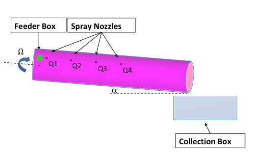
Figure 1: DEM simulation setup for a continuous impregnation process.

Figure 1 shows the simulation setup. A full-length rotating cylinder with a given inclination angle and RPM, and a series of nozzles (1 to 4 nozzles) are used for the impregnation process. A feeder box is located at one end of the cylinder and a collection box at the other end. Particles are fed from the feeder box, flow through the cylinder, and are collected in the collection box. The residence time is defined as the time that particles stay inside the drum. The probability distribution of the residence time is the Residence Time Distribution (RTD). Figure 1 shows the depiction of the nozzle position along the axis. In this figure, $Q_{1}$ to $Q_{4}$ indicates the flow rates through the four nozzles respectively and $\alpha$ indicates the angle of inclination. The nozzles were selected to be in positions that are equally spaced at 10 cm from each other.

3 Results of DEM simulations

3.1 Effect of the Inclination Angle and the Rotational Speed

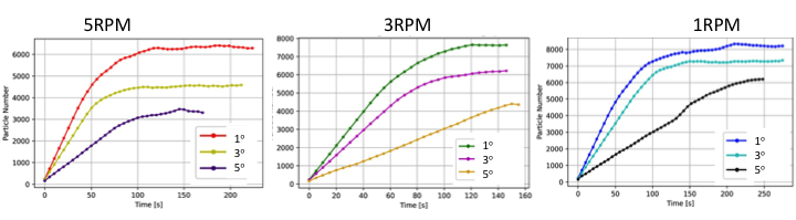
Figure 2: Number of particles as a function of time for different speeds.

We first studied the number of particles (NP) in the vessel. The mass holds up in the vessel is equal to the number of particles inside the cylinder. The mass hold up is dependent on the flow rate and it is the same for both patterns of flow rate. The number of particles in the cylinder is calculated and plotted as a function of time, see Figure 2. The number of particles in the cylinder first increases, and then reaches a plateau, which is considered a steady state.

We then examined the effect of inclination angle and rotational speed and how they affect the time to reach a steady state. We varied the inclination angle: 1, 3, and 5 degrees, and observed the time to reach a steady state within the cylinder. The first thing that we observe is that the number of particles inside the cylinder increases as the rotational speed decreases. The higher the rotational speed, the faster the steady state is reached and the shallower the bed is the smaller the number of particles. The number of particles inside the cylinder does not depend on the even or uneven distribution of flow rates. Let us analyze what happens for small and large speeds.

Figure 2 shows that at 1 RPM, for 1 degree, there are approximately 8,100 particles inside the drum, for 3 degrees there are roughly 7,000 particles inside the drum at steady state and for 5 degrees there are roughly 6,000 particles. This plot clearly shows that the larger the angle, the lower the number of particles that hold up in the cylinder at the steady state (i.e. the shallower the bed) and the sooner the steady state is reached.

At high speeds, at 5 RPM, for 1 degree, there are approximately 6,200 particles inside the drum, for 3 degrees there are roughly 4,500 particles inside the drum at the steady state and for 5 degrees there are roughly 3,200 particles. This plot clearly shows that the larger the angle, and the larger the speed, the lower the number of particles that hold up in the cylinder at the steady state (i.e. the shallower the bed) and the sooner the steady state is reached.

3.2 Behavior After Steady State

After reaching steady state, we focused on calculating the residence time distribution of the particles. Residence time (RT) is defined by the time interval between feeding and draining. For impregnation, the time that particles stay under the spraying zone directly depends on the RT. Tracer particles are “injected” at the inlet after steady state is reached by labeling a specific set of particles. Equation (1) shows the residence time distribution, $E(t)$:

$$E(t)=\frac{C(t)}{\int_{t=0}^{\infty}C(t)dt},$$ (1)

where $C(t)$ is the concentration of tracer particle at the outlet as a function of time. While the mean residence time (MRT) can be predicted by Sullivan’s model:

$$MRT=\frac{\sqrt{\phi}Lf}{\alpha D\omega}.$$ (2)

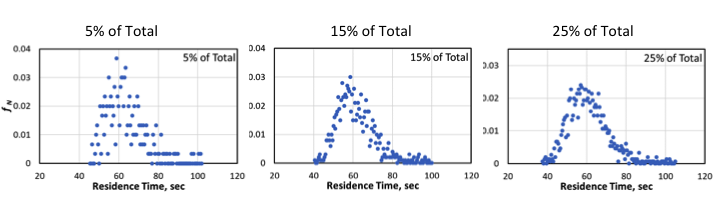
Figure 3: Residence time distribution for different amount of tracer particles used.

In Eq. (2), $\phi$ is the angle of repose, $D$ and $L$ are the diameter and length of the cylinder, $\alpha$ is the inclination angle, $\omega$ is the rotational speed. The quantity of tracer was chosen to have a good RTD. Different percentages of tracer particles (w.r.t. Total Number of Particles) were tested. Figure 3 shows the RTD for different tracer particle amounts. For a smaller ratio of tracer particles, the RTD shows scattered points. For a larger ratio of tracer particles, the RTD looks good, but it needs more computational time. Therefore, it was found that a convenient number for the tracer particles is 15% of the total number of particles. Similar ratios for the tracer particles were used by Gao et al. [13].

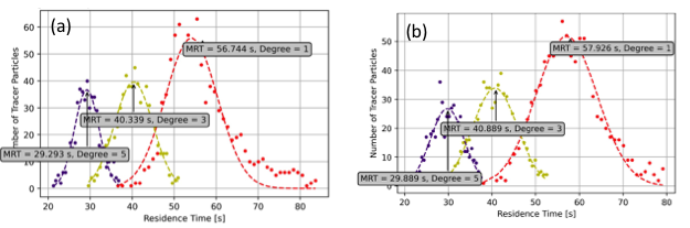
Figure 4: Residence time distribution of tracer particles in a continuous impregnator for 5 RPM at different inclinations angles, (1, 3 and 5 degrees) for (a) uneven pattern (b) even pattern. The points are the simulation results, and the dash curves are fittings with a Gaussian function.

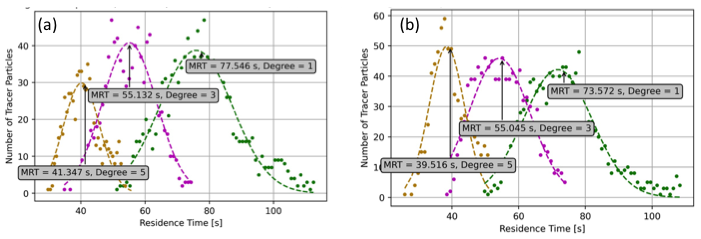
Figure 5: Residence time distribution of tracer particles in a continuous impregnator for 3 RPM at different inclinations angles, (1, 3 and 5 degrees) for (a) uneven pattern (b) even pattern.

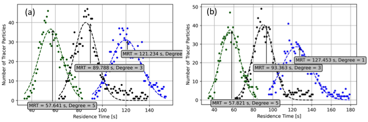
Figure 6: Residence time distribution of tracer particles in a continuous impregnator for 1 RPM at different inclinations angles, (1, 3 and 5 degrees) for (a) uneven pattern (b) even pattern.

We then examined the effects of rotational speed and inclination angle on the mean residence time (MRT). Figures 4, 5 and 6 show the plot of the tracer particles for 5 RPM, 3 RPM, and 1 RPM respectively as a function of the residence time, for even and uneven patterns.

For example, looking at the plot in Figure 4 for a fixed rotational speed (5rpm), the mean residence time (MRT) increases for smaller angles of inclination. In other words, the smaller the angle of inclination, the larger the MRT, which is consistent with Sullivan’s prediction. Particles stay in the cylinder for a longer time when the inclination angle is smaller. These findings are also reflected for the other speeds. In other words, all the results shown in Figures 4, 5 and 6 show that the larger the angle, the smaller the MRT, and the larger the speed of rotation, the smaller the MRT. The results reflect that Sullivan’s model can successfully predict the MRT as particles flow through the cylinder.

We then examined the water content of the tracer particles.

It is noticeable that the larger the number of particles inside the cylinder (i.e. the larger the mass holdup) the longer it takes to reach 100 percent saturation. We also observe that the uneven distributions reach 100 percent faster than the even distributions for all cases.

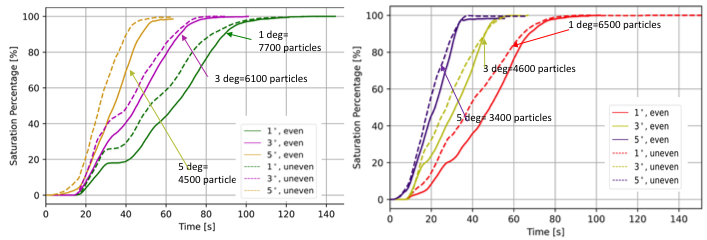
Figure 7: Percentage of pore filling of the tracer particles as a function of time for (a) 3 RPM and (b) 5 RPM.

The larger the MRT, the longer it takes to reach uniformity. This is not surprising, because as we see in Figure 7a the longest MRT corresponds to 1 degree. At this angle, the number of particles inside the cylinder is very high ($\sim$7,700). This is one of the highest beds possible and for that reason it takes the longest time to fill the pore volume. Notice that the yellow curve in Figure 7a corresponds to $5^{\circ}$ ($\sim$4,500 particles). It has fewer particles inside the cylinder, so it takes less time to reach full pore volume at saturation. Notice also that the two systems that have similar MRT (even and uneven) reach uniformity at a similar time (solid and dash lines). Figure 7b shows that the larger the MRT, the better the RSD as was found previously.

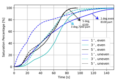
Figure 8: Percentage of pore filling of the tracer particles for 1 RPM considered as a function of time for 1, 3, and 5 degrees for even and uneven flow rate patterns.

We also did the case of 1 RPM. Results are shown in Figure 8. For 1 RPM, we also observe that the uneven distributions reach 100 percent faster than the even distributions. However, for 1 RPM only after 60 seconds it is possible to observe the expected trend that higher angles reach saturation faster (or vice versa: smaller angles take more time to reach saturation).

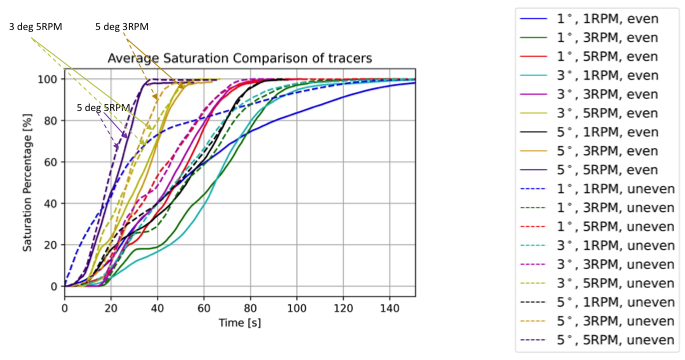
Figure 9: Percentage of pore filling of the tracer particles for all cases considered as a function of time for 1 RPM, 3 RPM and 5 RPM, for 1, 3 and 5 degrees for even and uneven flow rate patterns.

Figure 9 shows all the cases considered. We corroborate that for higher drum speeds and higher angles the system reaches saturation faster. As always, we can observe that the uneven pattern configurations reach saturation faster than the even patterns of flow rates. Higher rates and/or inclinations result in particle beds that are so shallow that some of the sprays misses the bed.

3.3 Relative Standard Deviation: Comparison of Even and Uneven Distribution of Flow Rates

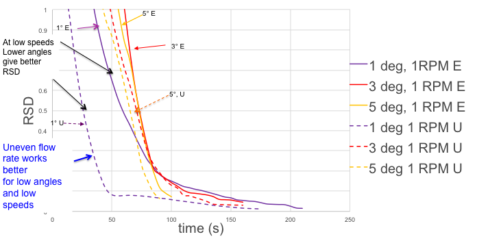
Figure 10: Plot of RSD of tracers for both even and uneven for $\Omega=1$.

Figure 10 shows that for rotational speeds lower angles give a better RSD as shown by the black arrows for both even and uneven flow rates. We also see that at low angles of inclination (1 degree) there is a dense packing of particles at the beginning of the vessel because the bed height is higher. So uneven flow rates favor uniformity in this case.

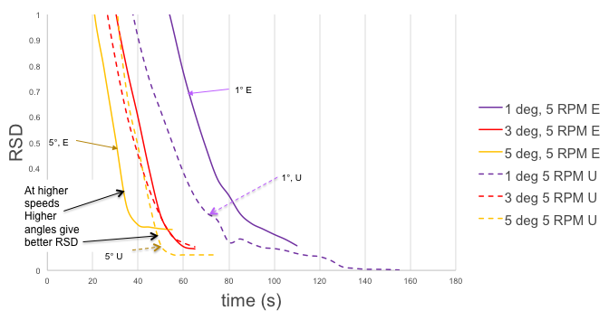
Figure 11: Plot of RSD of tracers for both even and uneven for $\Omega=5$.

Figure 11 shows that at high speeds and higher angles, RSD drops very quickly however the final values are not necessarily the lowest as it can be observed in the solid yellow line and the dashed yellow line. We see however that for high speeds and low angles (1 degree even and uneven), the RSD takes more time to drop (Distance from the y axis is much longer) but the final value of the RSD is a lot smaller as can be seen in the purple dashed and purple solid lines because the MRT is a bit larger.

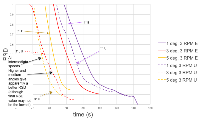
Figure 12: Plot of RSD of tracers for both even and uneven for $\Omega=3$.

Figure 12 shows that at intermediate rotational speeds we observe a somehow similar behavior to high speeds. For higher and medium angles RSD has a quick drop but they do not give the smallest RSD values. For low angles, medium speed such as 3 RPM does not provide enough mixing for the large packing at the left so RSD does not drop too quickly, however, MRT is large so ultimately RSD has the lowest values.

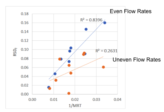
Figure 13: $RSD_{f}$: Value of the RSD when all tracers exit the vessel(at $t_{f}$).

We also plotted the RSD of the tracers as a function of 1/MRT in Figure 13. In this figure we observe a lower (better) RSD at higher MRT: more time, better product. This figure also shows that the RSD values for even flow rates nicely follow the trend of 1/MRT. When we use uneven flow rates, RSD is not a monotonic function of 1/MRT. In most cases, the RSD of tracer particles at the time the final tracer particle exits the vessel ($RSD_{f}$) will decrease if MRT increases. Increasing MRT means particles remain in the vessel longer. Particles have more exposure to water and more time to mix. So, increasing either RPM or angle of inclination results in lower MRT and higher RSD (in most cases). In general, uneven flow rate distributions improve $RSD_{f}$. For uneven flow rate cases, sufficiently high RPM appears to compensate the decrease in MRT, resulting in improved $RSD_{f}$.

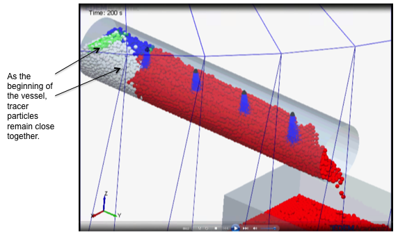
Figure 14: Snapshot of 1 degree, 1 RPM uneven at 200 seconds. At the beginning, tracer particles remain close together.

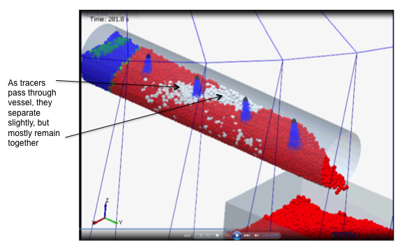
Figure 15: Snapshot of 1 degree, 1 RPM, uneven at 281 seconds. We observe that as tracers pass through the vessel, they separate slightly, but mostly remain together.

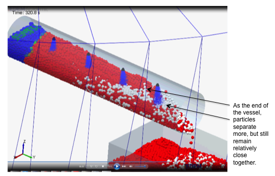
Figure 16: Snapshot of 1 degree, 1 RPM, uneven at 320 seconds. At the end of the vessel, particles separate more but still remain relatively close together.

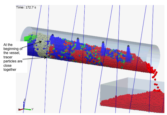
Figure 17: Snapshot of 1 degree, 5 RPM, uneven at 172.7 seconds. At the beginning of the vessel, tracer particles are close together.

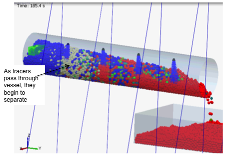
Figure 18: Snapshot of 1 degree, 5 RPM uneven at 185.4 seconds. As tracers pass through the vessel, they begin to separate.

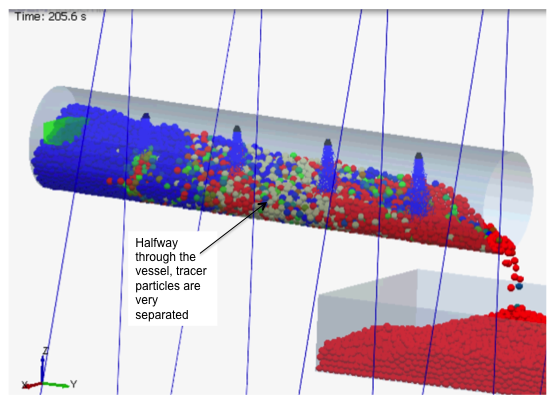
Figure 19: Snapshot of 1 degree, 5 RPM, uneven at 205.6 seconds. Halfway through the vessel, tracer particles are very separated.

Figures 14 to 19 show different snapshots of the system at different times. Figure 14 shows a snapshot of the system at 200 seconds and low speed of the vessel (1RPM). We observe that tracer particles remain close together at the begining of the vessel. Figure 15 shows a snapshot at 281 seconds where we can see that tracers pass through the vessel, they separate slightly but remain mostly together. A 320 seconds particles separate a bit more but still remain relatively close together (see Figure 16). As we increase the speed of the vessel to 5RPM we observe the same characteristics at the beginning of the vessel (Figure 17): particles remain close together and as they pass through the vessel they separate and until they are mostly mixed (see Figures 18 and 19).

From Figures 14 to 19 we observed that the bed appears to contain two regimes:

• Regime 1. This appears towards the beginning of the vessel. Here, neighboring particles tend to remain close together, and the height of the bed is large.

• Regime 2: As tracer particles move through vessel, they tend to mix. Towards the end of the vessel, particles that were close together in the beginning of the vessel are now mixed and the height of the bed is more shallow.

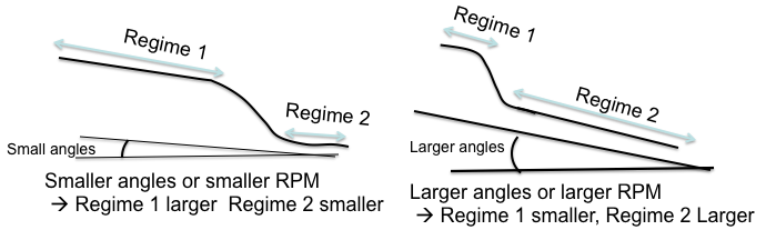
Figure 20: Schematic of different regimes observed at different RPM and different angles.

Figure 20 shows a schematic of the different regimes observed at different rotational speeds and different angles. The two regimes in the vessel should be treated differently. More water should be sprayed in regime 1, where neighboring particles remain close together. Particles will be exposed to similar amounts of water and have more time to exchange fluid. Less water should be sprayed in regime 2: water content uniformity will be benefited by water exchange between particles. We obtained better results when 70% of the total amount of fluid is sprayed in regime 1 and 30% in regime 2.

We also observed that the size of the regimes is a function of inclination angle and RPM. More RPM generates more mixing and therefore will decrease the size of regime 1 and increase the size of regime 2 (mixing regime). Smaller inclination angles generate a larger mass hold-up with stronger forces restricting the particle movement. Larger inclination angle and/or RPM generate a smaller mass holdup and therefore a smaller bed height, consequently a smaller regime 1 and a larger regime 2.

4 Machine Learning

In order to elucidate the role of the parameters that affect the process of continuous impregnation we use machine learning regressions. Machine learning is a type of artificial intelligence that allows software applications to become more accurate at predicting outcomes without being explicitly programmed to do so. Machine learning algorithms use data as input to predict new output values. We focus on processing the data we got for different values of RPM, angles of inclination, the final time for tracers, and flow patterns, even and uneven. There are different approaches to fit the experimental data and build the regressed function such as LASSO (Least Absolute Shrinkage and Selection Operator) [28], MARS (Multivariate Adaptive Regression Splines) [28], and Neural Network Deep Learning. Particularly the neural network usually requires many samples which we don’t have. Between LASSO and MARS, we employed LASSO since it gives higher accuracy compared to MARS in our case. The LASSO method is a regression analysis method that performs both variable selection and regularization in order to enhance the prediction, accuracy, and interpretability of the resulting statistical model [28].

4.1 Procedure using the LASSO Method

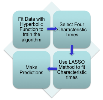
Figure 21: Schematic of the method followed to use the LASSO method.

We follow the scheme depicted in Figure 21, as follows. From the simulations we obtained RSDs as functions of time for samples with different parameters (inclination degree and rotation speed). We first fit these data using hyperbolic functions. Then we select four characteristic times and use the LASSO method [28] to fit those characteristic times from the parameters. In the end, we make predictions with fitted functions and new parameters to get new characteristic times, thus RSD vs. time curves of new parameters can be determined.

4.1.1 Data Fitting with Hyperbolic Function: Even and Uneven Spraying

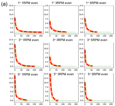
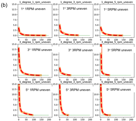
Figure 22: Fitted hyperbolic functions and data point for (a) even and (b) uneven cases. The dashed lines are the fitted hyperbolic function and the orange lines are the real Data.

The first step is to get a hyperbolic function that fits the data to have a continuous curve, since the data points are discrete and we need a continuous curve to predict new values. Figure 22 shows the fitted hyperbolic functions for (a) even, and (b) for uneven spraying cases.

The hyperbolic function (red dashed line) in Figure 22 was used to fit the RSD discrete data points obtained from our experiments by using the following equation:

$$RSD(t)=\frac{a}{t+b}+c.$$ (3)

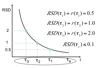
Figure 23: Schematic of the Relative Standard Deviation as a function of time showing the different characteristic times $\tau_{1}$, $\tau_{2}$, $\tau_{3}$, and $\tau_{e}$. Each of these times are chose according to: RSD($\tau_{1}$)= 0.5 , RSD($\tau_{2}$)= 1 , RSD($\tau_{3}$)= 2 , and RSD($\tau_{e})<0.1$ .

An hyperbola described by the equation above is determined by three parameters $a$, $b$ and $c$. But, more generally, an hyperbola can be determined by any three points defined on it. In order to give parameters more realistic meanings, we extracted 3 characteristic times $\tau_{1}$, $\tau_{2}$, $\tau_{3}$, and also the final time $\tau_{e}$ at which all the tracers exit the vessel. We will use these four parameters to feed into the regression algorithm. Figure 23 shows the characteristic times that are located on the time axis, and each of these characteristic times corresponds to a pre-selected certain value of the RSD. The goal is to find the lowest $\tau_{1}$, $\tau_{2}$, and $\tau_{3}$ to obtain the highest quality product. Notice that lower values of $\tau_{e}$ relates to higher production rate.

We then considered two parameters to determine the RSD function for a simulation: the rotational speed $\Omega$ of our samples and the angle of inclination $\alpha$ of the vessel, for both even and uneven spraying. The goal is to find the functions $f^{1}$, $f^{2}$, $f^{3}$, and $f^{e}$, such that $\tau_{i}=f^{(i)}(\Omega,\alpha)$, where $i=1,2,3,e$.

In LASSO, functions $f^{(i)}$ are parameterized by $\beta$s in the following way:

$$\tau_{i}=\beta_{1}^{i}+\beta_{2}^{i}\Omega+\beta_{3}^{i}\alpha+\beta_{4}^{i}\Omega^{2}+\beta_{5}^{i}\alpha^{2}+\beta_{6}^{i}\Omega\alpha+\beta_{7}^{i}\Omega^{3}+\beta_{8}^{i}\Omega^{2}\alpha+\beta_{9}^{i}\Omega\alpha^{2}+\beta_{1}0^{i}\alpha^{3},$$

where $i=1,2,3$. Specifically, when fitting $f^{(e)}$ we expand it only to the second order of parameters since the fitting is already good enough so overfitting is avoided.

In the LASSO method [28], the idea is to make the fit small by making the residual squares small plus a penalty, in such a way that:

$$\min(\sum^{9}_{j=1}(\tau_{i,j}-\tau_{i,j}^{real})^{2}+\lambda\sum^{10}_{k=1}|\beta_{i,k}|),$$ (4)

where $i$ labels different characteristic time, $j$ labels all 9 samples we have, and $k$ labels 10 $\beta$s used in the fitting functions.

4.1.2 Predictions from Fitted Hyperbolic Functions

Once we have fitted functions we are able to predict three characteristic times from any given new parameters $\Omega$ and $\alpha$. Thus we can obtain the parameters $a$, $b$, and $c$ in the hyperbolic function from three characteristic times following:

$$b=\frac{\frac{\tau_{3}}{\tau_{3}-\tau_{2}}-\frac{\tau_{1}}{2(\tau_{2}-\tau_{1})}}{\frac{1}{2(\tau_{2}-\tau_{1})}-\frac{1}{\tau_{3}-\tau_{2}}},$$ (5)

$$a=-\frac{1}{2}(\frac{(\tau_{1}+b)(\tau_{2}+b)}{2(\tau_{2}-\tau_{1})}+\frac{(\tau_{2}+b)(\tau_{3}+b)}{\tau_{3}-\tau_{2}}),$$ (6)

$$c=\frac{1}{3}(\frac{7}{2}-\frac{a}{\tau_{1}+b}-\frac{a}{\tau_{2}+b}-\frac{a}{\tau_{3}+b}).$$ (7)

Using these values of $a$, $b$, and $c$ we are able to draw the full RSD vs time curve for intermediate values of all rotational speeds and angles within the limits of the parameters fed in the LASSO algorithm, as shown in Figure 24.

5 Results: Predictions from Machine Learning

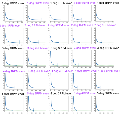
Figure 25: Even cases. Panels with purple titles are new predictions that were not included in the data fed to the LASSO algorithm (i.e. these cases were never run with DEM before).

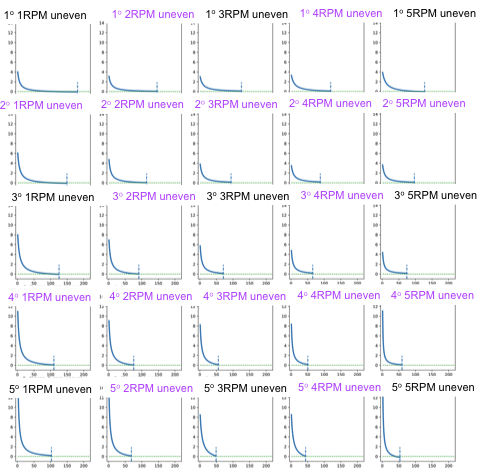
Figure 26: Uneven cases. Panels with purple titles are new predictions never run with DEM before. We can predict intermediate RPMs and angles. The decay of RSD is faster for uneven spraying.

In Figures 25 and 26 we depict our predictions for the even and uneven spraying cases. Using the RSD obtained as shown in Figures 25 and 26, we were able to make predictions using the LASSO algorithm for the even case and uneven cases respectively. Notice that the panels with titles in purple correspond to the new predictions of cases that were not included in the data fed to the algorithm (i.e. they were not run with DEM).

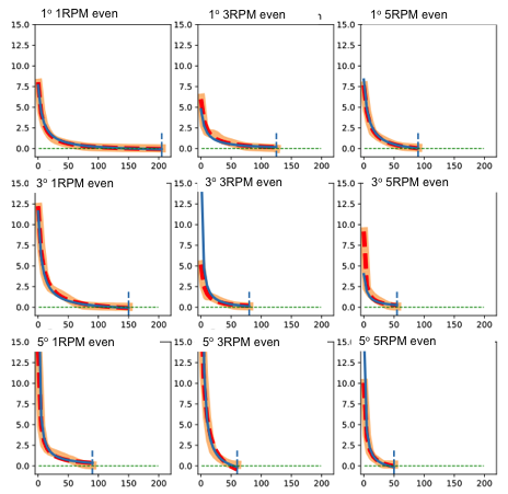
Figure 27: Even cases. Red Dashed: hyperbolic fit, Orange: Real Data, Blue: Prediction with LASSO. We observe great agreement with the original data.

With machine learning we can predict intermediate cases for other RPM values and angle values. We can observe in this figure that the decay of the RSD is faster for uneven spraying in general. Predictions need to be checked for accuracy against the data and the fitted functions. Figure 27 shows the accuracy of the predictions compared to the experimental data and the fitted hyperbola for both even and uneven cases respectively.

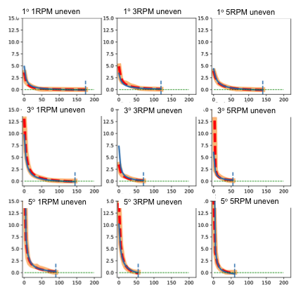
Figure 28: Uneven cases. Red Dashed: hyperbolic fit, Orange: Real Data, Blue: Prediction with LASSO. We observe great agreement with the original data.

In Figure 28 we present the data for uneven cases. There is great agreement with the original data and the fitted hyperbola. In these figures we can observe that for low RPM and low angles, when the bed is larger in particle density and displays a larger regime 1, the lower RSD values correspond to the uneven cases. And for the cases of large RPM and larger angles, when the particle bed is shallow and even and mostly in regime 2, the lower RSD values correspond to the even spraying scenario.

Figures 27 and 28 show that the larger the RPM the longer it takes to achieve uniformity as seen for the cases of RPM =1. It is interesting to notice that a slight increase in the angle for high RPM reduces the time of uniformity by 3 as can be observed when comparing 5 RPM and 1 degree with 5 RPM and 3 degrees.

5.1 Qualitative Study of Regime 1 and Regime 2

We can get a qualitative estimation of the distribution of the regimes by looking at the particle densities in the cylinder. The particle density $\phi$ is calculated using the feeding rate (100 particles/second), the particle diameter $d$, the cylinder’s diameter and length $D$ and $L$, and the MRT as:

$$\phi=\frac{NV_{part}}{V_{drum}}=\frac{100\ part/s\ MRT\ V_{part}}{V_{drum}}=\frac{100MRT\frac{4}{3}\pi(d/2)^{3}}{\pi(D/2)^{2}L}=\frac{200d^{3}MRT}{3D^{2}L}$$

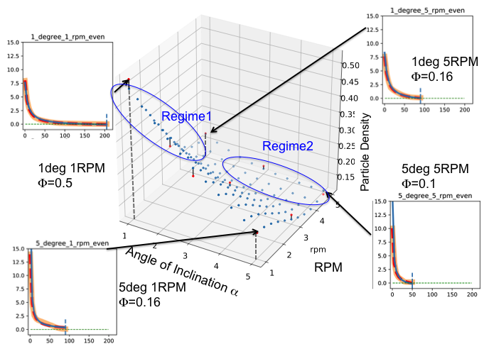
Figure 29: Even case. Regimes do not depend on the spray pattern. Regimes depend on the MRT.

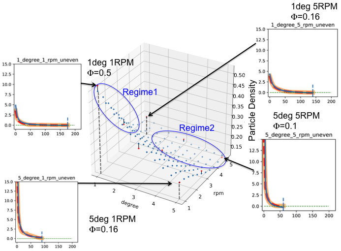
Figure 30: Uneven case. Regimes do not depend on the spray pattern. Regimes depend on the MRT.

Figure 29 shows qualitatively the two different regimes, 1 and 2. Notice that for small angles of inclination and small RPM, the particle density is the highest as indicated by the dashed line $\phi=0.5$. We can see that the large values of the density extend until 3 RPM and 1 degree of inclination. The RSD for these cases is not the lowest, as indicated by the two insets. If we compare these values with the same values in Figure 30 we see that uneven spraying works better. That is because when there is larger density of particles it is better to use uneven spraying, more water at the very left of the vessel to saturate the large accumulation of particles.

Larger angles of inclination do not show a great accumulation of particles. We can also observe in this figure that for 5 degrees and 1 RPM ($\phi=0.16$) and 5 degrees, 5 RPM, ($\phi=0.1$) the density of particles is the lowest indicating that the system is in regime 2. We would expect that for this regime the even distribution would give a lower RSD compared to the uneven spraying. This can be seen in Figure 30 in the inset 5 deg 5 RPM, where the RSD for uneven spraying has a higher value than for the even case depicted in Figure 29.

5.2 Fitting functions found by LASSO

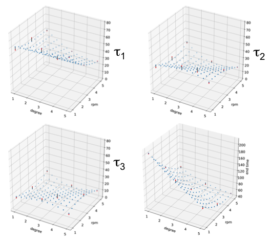
Figure 31: Even cases. $\tau_{1}$, $\tau_{2}$, $\tau_{3}$ and $\tau_{e}$ as functions of $\Omega$ and $\alpha$.

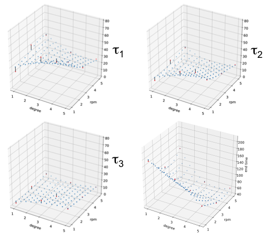
Figure 32: Uneven cases. $\tau_{1}$, $\tau_{2}$, $\tau_{3}$ and $\tau_{e}$ as functions of $\Omega$ and $\alpha$.

As mentioned earlier the goal is to predict $\tau$s that depend on the rotational speed and the angles. Figures 31 and 32 below shows the functions found by the LASSO algorithm for the even cases and uneven cases.

Notice that low values of $\tau_{1}$, $\tau_{2}$ and $\tau_{3}$ relate to high quality product. Also, lower $\tau_{e}$ relates to a higher production rate. In Figure 32, in general for uneven spraying cases, we observe a faster decay of the RSD.

Functions found by LASSO: $\tau_{1}$

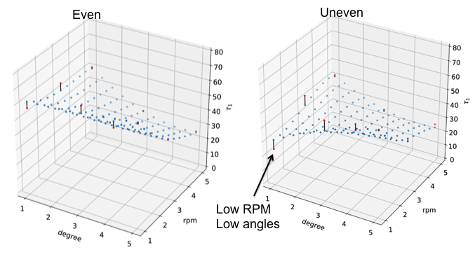
Figure 33: Comparison side by side of the plots of $\tau_{1}$ as a function of RPM and angle of inclination (a) even, (b) uneven.

Figure 33 depicts the plots of $\tau_{1}$ as a function of RPM and angle of inclination. We can observe that for uneven cases (b), $\tau_{1}$ reveals that for low RPM in general gives lower RSD. Also, this confirms that for low RPM and low angles uneven gives better RSD as we had concluded with our DEM simulations.

Notice that, in the inset of Figure 33 we can observe that the smallest the value of $\tau_{1}$, the faster RSD decays to zero, indicating a better quality of the product.

Functions found by LASSO: $\tau_{2}$

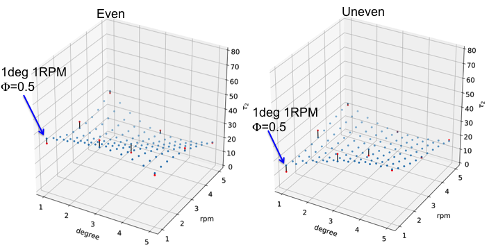
Figure 34: Comparison side by side of the plots of $\tau_{2}$ as a function of RPM and angle of inclination (a) even, (b) uneven.

Figure 34 shows the function $\tau_{2}$ found with the LASSO algorithm as a function of RPM and angle of inclination. We can observe that for 1 degree and 1RPM, low angles and low velocities of the drum, the uneven spraying gives a lower value of the RSD. This makes sense because at low angles and low velocities there is a larger Regime 1, therefore, an uneven distribution of the spraying should give a more uniform distribution to counteract the accumulation of particles at the left of the vessel.

Functions found by LASSO: $\tau_{3}$

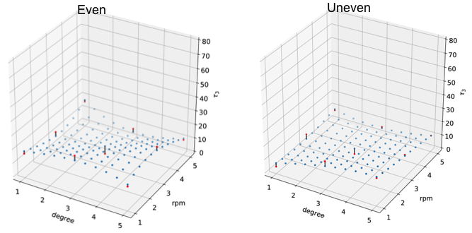
Figure 35: Comparison side by side of the plots of $\tau_{3}$ as a function of RPM and angle of inclination (a) even, (b) uneven.

Figure 35 shows the function $\tau_{3}$ found with the LASSO algorithm as a function of RPM and angle of inclination. We see that in general for uneven spraying we observe a faster decay (quick drop) of the RSD.

Functions found by LASSO: $\tau_{e}$

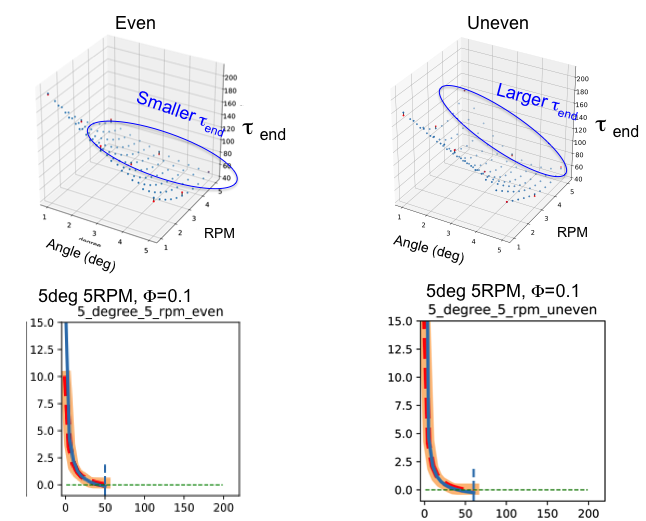
Figure 36: Comparison side by side of the plots of $\tau_{e}$ as a function of RPM and angle of inclination (a) even, (b) uneven.

Figure 36 corresponds to $\tau_{e}$. In Figure 36(a) we see that for even spraying, the smaller values of $\tau_{e}$, which indicate a really good uniformity since RSD would decay very quickly, correspond to the highest values of the speed of drum (high RPM) for any value of the angle of inclination. This may indicate that when the speed of the drum is high, the height of the bed tends to even out, and for high angles is shallow and leveled off. Therefore, even spraying will provide more uniformity than uneven spraying. Notice that for high RPM and high angles the $\tau_{e}$ is really small in value indicating that the RSD decays very quickly. This happens for both even and uneven although if we observe the curves closely, the lowest value of tend for high RPM and high angles occurs for even spraying.

6 Conclusions

We developed a DEM framework for a systematic study of the continuous impregnation process. This framework allows to test and optimize the effect of various parameters, such as the number of nozzles, the nozzle spacing, the angle of inclination of the vessel, the wetted area, the drum speed, the flow rate patterns, etc.

During startup, the number of particles inside the cylinder first increases and then reaches a steady state value. The higher the rotational speed and the higher the inclination angle, the sooner the steady state is reached and the shallower the bed is.

In all our studies, we see that the effects of inclination angle and rotational speed are consistent with Sullivan’s prediction: the MRT is inversely proportional to the angle of inclination and rotational speed. However, more studies are needed to elucidate the role of the wetted area. The RSD for the water saturation of the tracers reveals some general trends. We observe that at low rotational speeds lower angles give better RSD. At high speeds higher angles give a quick drop in RSD however they do not yield the lowest values of the RSD. At low angles and low rotational speeds uneven flow rate helps to have a lower RSD due to the large packing of the particles at the beginning of the vessel.

Using machine learning we found a general function for the relative standard deviation as a function of time, $\alpha$, $\Omega$ and for both even and uneven flow rates. We are able to predict the full RSD vs time for intermediate values of all rotational speeds and angles within the limits of parameter values fed in the LASSO algorithm. In general for uneven spraying we observe a faster decay of the RSD which should give a better product quality. That is evident with the value of $\tau_{1}$ and $\tau_{2}$ being lower for the uneven flow rate pattern in general. Machine learning also reveals that for low RPM and low angles, since the particles are mostly in the regime 1, uneven spraying yields much lower values of the RSD (better product quality), which is consistent with our previous observations of the DEM snapshots. We see that for high RPM and high angles (particles within the vessel are in regime 2), the particle bed is very shallow and even works better (characteristic times are smaller). We also verify that regimes do not depend on the spray pattern but on the MRT, as it was expected. The recommendation is to use uneven spraying unless the bed is purely in Regime 2. Ultimately we developed a computational framework that could find optimal performance within the parameter space.

Author contributions: KL performed the machine learning calculations, YS and JS performed the DEM simulations, BB advised on the project, HAM directed the machine learning part, and MST performed some of the DEM simulations wrote the paper and directed the project.

Funding source: This work was funded by the Rutgers Catalyst Manufacturing Consortium (RCMC) and NSF DMR-1945909.

Figure 24: Schematic of the process followed to find the RSD as a function of the characteristic time.

References

- [1] James A. Schwarz, Methods for preparation of catalytic materials, Chemical Reviews, 95, 477-510, 1995.
- [2] A.J. van Dillen, R.J.A.M. Terörde, D.J. Lensveld, J.W. Geus, K.P. de Jong, Synthesis of supported catalysts by impregnation and drying using aqueous chelated metal complexes, Journal of Catalysis, 216, 257-264, 2003.
- [3] L. Barthe, S. Desportes, M. Hemati, K. Philippot, B. Chaudret, Synthesis of supported catalysts by dry impregnation in fluidized bed, Chemical Engineering Research and Design, 85, 767-777, 2007.
- [4] Gluba, T., Kochaski, B., Water penetration into the bed of fine-grained materials, Physicochemical Problems of Mineral Processing, 39, 67-76, 2005.
- [5] Danov K.D., Pouligny B., Kralchevsky P.A., Capillary forces between colloidal particles confined in a liquid film: the finite-meniscus problem, Langmuir, 17, 6599-6609, 2001.
- [6] Lekhal, A., Conway, S.L. Glasser, B.J., Khinast, J.G., Characterization of granular flow of wet solids in a bladed mixer, AICHE Journal, 52, 2757-2766, 2006.
- [7] Peter Munnik, Petra E. de Jongh, and Krijn P. de Jong, Recent developments in the synthesis of supported catalysts, Chemical Reviews, 115, 6687-6718, 2015.
- [8] Lekhal, A., Glasser, B.J., and Khinast J.G., Influence of ph and ionic strength on the metal profile of impregnation catalysts, Chem. Eng. Sci., 59, 1063-1077, (2004).
- [9] Liu, X., Khinast, J.G. and Glasser, B.J., A Parametric Investigation of Impregnation and Drying of Supported Catalysts, Chem. Eng. Sci., 63, 4517-4530, (2008).
- [10] Kumar et al. Inter-particle coating variability in a continuous coater, Chemical Engineering Science, 117, 1-7 (2014).
- [11] Dubey et al. Impact of process parameters on critical performance attributes of a continuous blender: A DEM-based study, AIChE Journal, 58, 3676-3684 (2012).
- [12] Gao et al. Periodic section modeling of convective continuous powder mixing processes, AIChE Journal, 58, 69-78 (2012).
- [13] Gao et al. Optimizing continuous powder mixing processes using periodic section modeling, Chemical Engineering Science, 80, 70-80, 2012.
- [14] Sarkar et al. Comparison of flow microdynamics for a continuous granular mixer with predictions from periodic slice DEM simulations, Powder Technology, 221, 325-336 (2012).
- [15] Suzzi et al. DEM simulation of continuous tablet coating: Effects of tablet shape and fill level on inter-particle coating variability, Chemical Engineering Science, 69, 107-121 (2012).
- [16] Shirazian et al. Continuous twin screw wet granulation: The combined effect of process parameters on residence time, particle size, and granule morphology, Journal of Drug Delivery Science and Technology, 48, 319-327 (2018).
- [17] Behjani et al. An investigation on process of seeded granulation in a continuous drum granulator using DEM, Advanced Powder Technology, 28, 2456-2464 (2017).
- [18] Weber, M. W., D. K. Hoffman, and C. M. Hrenya, Discrete-particle simulations of cohesive granular flow using a square-well potential, Granular Matter, 6, 239-254 (2004).
- [19] LaMarche, C. Q., P. Liu, K. M. Kellogg, A. W. Weimer, and C. M. Hrenya, A system-size independent validation of CFD-DEM for noncohesive particles, AICHE Journal, 61, 12, 4051-4058, 2015.
- [20] B. Chaudhuri, A. Mehrotra, F.J. Muzzio, M.S. Tomassone, Cohesive effects in powder mixing in a tumbling blender, Powder Technology 165 (2) (2006) 105–114.
- [21] A. Faqih, B. Chaudhuri, A.W. Alexander, C. Davies, F.J. Muzzio, M. Silvina Tomassone, An experimental/computational approach for examining unconfined cohesive powder flow, International Journal of Pharmaceutics 324 (2) (2006) 116–127.
- [22] E. Sahni, R. Yau, B. Chaudhuri, Understanding granular mixing to enhance coating performance in a pan coater: experiments and simulations, Powder Technology 205 (1–3) (2011) 231–241.
- [23] Shi, D., Vargas, W. L., and Mccarthy, J. J., Heat transfer in rotary kilns with interstitial gases, Chemical Engineering Science, 63, 4506-4516, 2008.
- [24] Shi. D., McCarthy, J. J., Numerical simulation of liquid transfer between particles, Powder Technology, 184, 64-75, 2008.
- [25] Romanski, F. S., Dubey, A., Chester, A. W., Tomassone, M. S., Dry catalyst impregnation in a double cone blender: A computational and experimental analysis, Powder Technology, 221, 57-69, 2012.
- [26] A. Chester, J. Kowalski, M. Coles, E. Muegge, F. Muzzio, D. Brone, Mixing dynamics in catalyst impregnation in double cone blenders, Powder Technology, 102, 85-94, 1999.
- [27] Brone, D., Muzzio, F.J., Enhanced mixing in double-cone blenders, Powder Technology, 110, 179-189, 2000.
- [28] T. Hastie, R. Tibshirani, and J. Friedman, The Elements of Statistical Learning: Data Mining, Inference, and Prediction, Springer Series in Statistics (Springer New York, 2013).