Quantum states in disordered media. I. Low-pass filter approach

Abstract

The current burst in research activities on disordered semiconductors calls for the development of appropriate theoretical tools that reveal the features of electron states in random potentials while avoiding the time-consuming numerical solution of the Schrödinger equation. Among various approaches suggested so far, the low-pass filter approach of Halperin and Lax (HL) and the so-called localization landscape technique (LLT) have received most recognition in the community. We prove that the HL approach becomes equivalent to the LLT for the specific case of a Lorentzian filter when applied to the Schrödinger equation with a constant mass. Advantageously, the low-pass filter approach allows further optimization beyond the Lorentzian shape. We propose the global HL filter as optimal filter with only a single length scale, namely, the size of the localized wave packets. As an application, we design an optimized potential landscape for a (semi-)classical calculation of the number of strongly localized states that faithfully reproduce the exact solution for a random white-noise potential in one dimension.

I Introduction

Disordered semiconductors are in the focus of intensive experimental and theoretical research because these materials are successfully applied in various devices, and promise many fruitful applications in the future [1]. The term ‘disordered materials’ usually describes amorphous organic and inorganic solids without perfect crystalline structure. However, multi-component crystalline semiconductors with random atomic occupancies also belong to the broad class of disordered materials.

Alloying semiconductors is often used to tune material properties, such as band gaps and effective masses of charge carriers, depending on the device application. The price for this tunability is the extra disorder caused by spatial fluctuations in the distributions of the material components. These compositional fluctuations cause spatial fluctuations of the band gap which in turn create a random potential ${\cal V}(\vec{r}\,)$ acting on electrons and holes [2, 3]. The random potential leads to the spatial localization of charge carriers in electronic states at low energies.

It is desirable to develop theoretical techniques for an appropriate treatment of such localized states. A complete solution of the Schrödinger equation to obtain all localized states is too time-consuming. Therefore, theoretical tools to obtain the essential features of localized states without solving the Schrödinger equation are of extreme value. One of such tools is the recently introduced ‘localization landscape theory’ (LLT) [4, 5, 6, 7].

The LLT can be applied to any wave operator, quantum or classical. In the case of the Schrödinger equation, the localization-landscape potential can be seen as a regularization of the original potential, and provides an efficient access to the features of the low-energy localized states. The random potential ${\cal V}(\vec{r}\,)$ is converted into the ‘effective potential’ $W(\vec{r}\,)\equiv u^{-1}(\vec{r}\,)$, where $u(\vec{r}\,)$ is the solution of the LLT equation

$$-\frac{\hbar^{2}}{2m}\Delta u(\vec{r}\,)+{\cal V}(\vec{r}\,)u(\vec{r}\,)=1\;,$$ (1)

where $m$ is the carrier mass, $\hbar$ is the reduced Planck constant, and $\Delta$ is the Laplace operator. The LLT potential $W(\vec{r}\,)$ is then used to describe, e.g., the spatial dependence of the band edge $E_{c}(\vec{r}\,)$ [4, 5, 6, 7].

The LLT is widely considered as one of the efficient theoretical approaches to calculate the local density of states in disordered systems, for instance, in GaN-based light emitting diodes (LEDs) [8, 9]. The LLT has been used to simulate the carrier effective potential fluctuations induced by alloy disorder in InGaN/GaN core-shell microrods [10] and for direct modeling of carrier transport in multi-quantum-well (QW) LEDs [11] and in a type-II superlattice InAs/InAsSb photoconductor system [12]. The LLT is considered to be a promising approach to simulate random alloy effects in III-nitride LEDs [13], to connect atomistic and continuum-based models of III-nitride QWs [14], and to simulate carrier escape in InGaN/GaN multiple QW photodetectors [15]. Furthermore, the LLT has been applied to compute the eigenstate localization length at very low energies in two-dimensional disorder potentials [16]. Occasionally, the LLT is considered capable to reveal errors in the finite-element method software in applications to alloys [17]. It is also used for a three-dimensional modeling of minority-carrier lateral diffusion length in (In,Ga)N and (Al,Ga)N QWs and to analysis of light-emission polarization ratio in deep-ultraviolet LEDs by considering random alloy fluctuations [18, 19]. Moreover, the LLT frequently serves as a decisive ingredient in quantum-corrected drift-diffusion models [20, 21, 22].

Several attempts to extend and improve the LLT approach have been made. Chaudhuri et al. [23] suggested to search for the effective potential $W(\vec{r}\,)$ replacing Eq. (1), $\widehat{H}u=1$, by the equation $\widehat{H}^{2}u=1$. This improves the convergence of the calculated energies and the robustness of the method against the chosen integration region for $u$ to obtain the corresponding energies. Balasubramanian et al. [24] extended the LLT, developed initially for the single-particle Schrödinger operator, to a wide class of interacting many-body Hamiltonians. Steinerberger and collaborators [25, 26, 27] suggested to replace the LLT effective potential by a convolution of the initial random potential with a kernel function arising from a random Brownian motion. Altmann et al. [28, 29] and Jia and coworkers [30] addressed the relation between the LLT and Anderson localization problem. Harrell and Maltsev adapted the LLT approach for the eigenfunctions of quantum graphs [31]. Chenn et al. [32] focused on studying the features of the localized wave functions in the framework of the LLT. Grubišić et al. [33] used the deep neural network model to study eigenmode localization in the framework of the LLT. Lemut et al. [34] adapted the LLT to construct the landscape functions for Dirac fermions. Herviou and Bardarson [35] generalized the LLT approach to eigenstates at arbitrary energies.

In view of the variety of applications and extensions, the foundations of the LLT and its accuracy deserve more consideration. For instance, Comtet and Texier have shown that LLT does not reproduce the energy spectrum for some simple exactly solvable models, namely for the Pieces model and for supersymmetric quantum mechanics [36]. The group of Witzigmann argued that the LLT is not practical because it is either not deterministic or requires expensive experimental data. They found that when the LLT is restricted to a numerically expensive three-dimensional simulation, it does not perform well in optimization or calibration [37]. In their work, the effect of compound disorder was investigated with a statistical model. This modelling was embedded into a multi-scale multi-population carrier-transport simulator to study its influence on the electronic features [37]. Therefore, the question arises how to justify, and systematically improve, the LLT for solid-state applications. In the present work, we elucidate the meaning of the LLT as a Lorentzian low-pass filter to the random potential, and propose and justify the Halperin-Lax filter as a generic improvement.

Already in the 1960s, Halperin and Lax [38] suggested to apply a filter to smooth the random potential. They used a variational approach to describe the shape of the low-energy tail in the density of states in a random potential. The absolute square of the wave function serves as their filter function, whereby the width of the wave function depends on the energy of the localized state [38]. Later, Baranovskii and Efros [39] addressed the same problem by a slightly different variational technique and confirmed the result of Halperin and Lax for the density of states in a random potential.

However, neither of the two groups considered the individual features of localized states but restricted themselves to the description of the tails of the density of states. In the present paper, we further develop the idea of Halperin and Lax [38] to show that a low-pass filter applied to a random potential permits to reveal the energy together with the spatial positions of low-energy localized states in disordered media.

Our paper is organized as follows. In Sec. II we briefly summarize and formalize the problem of localized states in disordered systems and recall the main ingredients of the localization landscape theory [4, 5, 6, 7]. In Sect. III we outline the low-pass filter approach and show that the localization landscape theory, applied to the Schrödinger equation, is equivalent to a low-pass filter of Lorentzian form. In Sec. IV we show that low-pass filters belongs to the class of variational approaches to the low-energy localized states, and discuss various local filters (Gauss, Gauss-Lorentz, Halperin-Lax) that permit to find energy and position of individual localized states from effective potentials without solving the Schrödinger equation. Finally, we extend our analysis to define the Halperin-Lax low-pass filter globally. Comparing with the results of numerical studies of the localization problem in one dimension, we show that the global Halperin-Lax filter is superior to the global Lorentzian low-pass filter used thus far within the framework of the LLT. Moreover, we construct a landscape potential that can be used for the semi-classical approximation of the density of states in the band tails. Concluding remarks are gathered in Sec. V. In appendix A, we concisely re-derive the exact integrated particle density for the case of a random white-noise potential in one dimension. In appendix B, we identify the generic energy and length scales of the localization problem.

The focus of the LLT and, concomitantly, the focus of the current paper is set on the features of the temperature-independent effective potential $W(\vec{r}\,)$. In the LLT, $W(\vec{r}\,)$ determines the space- and temperature-dependent electron distribution $n(\vec{r},T)$ that is used to derive the opto-electronic properties of disordered semiconductors [7]. However, the effective potential that describes a correct distribution $n(\vec{r},T)$ should also depend on temperature. In our subsequent paper [40] we present two powerful techniques to access $n(\vec{r},T)$ without solving the Schrödinger equation. First, we derive the density for non-degenerate electrons by applying the Hamiltonian recursively to random wave functions. Second, we obtain a temperature-dependent effective potential $W(\vec{r}\,,T)$ from the application of a universal linear filter to the random potential acting on the charge carriers in disordered media. Thereby, the full quantum-mechanical problem is reduced to the quasi-classical description of $n(\vec{r},T)$ in a temperature-dependent effective potential. Both approaches prove superior to the LLT when we compare our approximate results for $n(\vec{r},T)$ and for the carrier mobility at elevated temperatures with those from the exact solution of the Schrödinger equation [40].

II Localized states in disordered systems

We start with a short description of the physical setting and define a Hamiltonian to model localized states in disordered systems. Next, we summarize the essence of localization landscape theory.

II.1 Model

First, we motivate the Hamiltonian used for the description of quantum mechanical states deeply localized in the band tails. Second, we define some physical quantities such as the single-particle density of states that can be derived from the solution of the Schrödinger equation.

II.1.1 Hamiltonian

In ideal crystals, there are no impurities and vacancies in the lattice. As a consequence, Bloch’s theorem applies so that the perfectly periodic lattice potential leads to bands in reciprocal space with single-particle states that extend over the whole crystal [41]. In the vicinity of the lower band edge, the dispersion is parabolic so that we can describe the band states using the kinetic energy operator in the form

$$T^{\rm op}(\vec{r}\,)=-\frac{\hbar^{2}}{2m}\Delta=-\frac{\hbar^{2}}{2m}\sum_{i=1}^{d}\frac{\partial^{2}}{\partial r_{i}^{2}}\;,$$ (2)

where $m$ is the effective mass determined by the curvature of the band at the $\Gamma$-point; for simplicity, we assume that the band minimum lies at the $\Gamma$-point in reciprocal space in dimension $d$.

When a single impurity is added to such a system, an anti-/bound state forms above/below the upper/lower band edge, provided the impurity potential is strong enough. In the presence of a finite density of impurities and other lattice imperfections, the band edges smear out and the single-particle states in the band tails are spatially localized. When semiconductors are optically excited, the density of charge carriers is small and they readily relax into localized states. The trap states and their properties thus dominate the (hopping) transport in these materials [1].

In alloy semiconductors, the site occupancies randomly vary so that the charge carriers experience potential fluctuations on an atomic length scale, $\ell_{\rm pf}\sim 1\,\hbox{\AA}$. The Hamiltonian to describe charge carriers in the band tails is thus defined in position space by

$${\cal H}_{\rm R}(\vec{r}\,)=T^{\rm op}(\vec{r}\,)+{\cal V}_{\rm R}(\vec{r}\,)\;,$$ (3)

where ${\cal V}_{\rm R}(\vec{r})$ describes a specific realization of the fluctuating potential. To calculate measurable quantities, an average over many realizations ${\rm R}$ must be carried out.

Following Halperin and Lax [38], we consider a random potential which arises in the limit of a finite density of $\delta$-function scatterers. This is permitted because the strength ${\cal V}$ of the scattering potential is small compared to the band width which leads to a typical size of the localized wave packet $\ell_{\rm wp}\sim 10\,\hbox{\AA}$ that is large compared to the potential fluctuation scale, $\ell_{\rm wp}\gg\ell_{\rm pf}$. For an estimate of $\ell_{\rm wp}$ we introduce

$${\cal T}=\frac{\hbar^{2}}{2m\ell_{\rm wp}^{2}}$$ (4)

as the typical average kinetic energy of a localized state. The estimate (4) implies that, while the band width is of the order of several electron volts, the typical average kinetic energy ${\cal T}$ of a localized state is of the order of several ten milli-electron volts. Algebraic expressions for $\ell_{\rm wp}$ and ${\cal T}$ through the model parameters are given in eq. (117).

To be definite, we assume that the potential is characterized by Gaussian statistics (‘white noise’), i.e., the potential obeys $\langle{\cal V}_{\rm R}(\vec{r}\,)\rangle_{\rm R}=0$ with the auto-correlation function [38]

$$\langle{\cal V}_{\rm R}(\vec{r}\,){\cal V}_{\rm R}(\vec{r}\,{}^{\prime})\rangle_{\rm R}=\frac{1}{12}{\cal V}^{2}(\ell_{\rm pf})^{d}\delta\left(\vec{r}-\vec{r}\,{}^{\prime}\right)\equiv S\delta\left(\vec{r}-\vec{r}\,{}^{\prime}\right)\;,$$ (5)

where $\langle\ldots\rangle_{\rm R}$ indicates the average over many realizations ${\rm R}$ of the random potential and $S$ is the strength of the interaction.

Only the energetically lowest-lying states are relevant for charge transport at low carrier concentrations and low temperatures. Therefore, a third length scale becomes important, $\ell_{\rm hop}$, for the typically hopping distance a particle travels between two localized states. States that are spatially close but disparate in energy cannot be accessed due to the lack of activation energy. Therefore, a hopping event only takes place between localized sites that are close enough in space and in energy. Depending on temperature, $\ell_{\rm hop}\sim 100\,\hbox{\AA}$, or larger. In this work, we shall not discuss transport, and it suffices to state that localized states that are close in energy are typically separated in distance by $\ell_{\rm hop}\gg\ell_{\rm wp}$. The precise definition of $\ell_{\rm hop}$ can be found in the monograph by Shklovskii and Efros [42].

II.1.2 Numerical simulations

Since ${\cal T}$ is the relevant energy scale for the localized states and $\ell_{\rm wp}$ is the corresponding length scale, we consider the dimensionless Hamiltonian in $d$ dimensions

$$\bar{\cal H}_{\rm R}(\vec{x}\,)=-\sum_{i=1}^{d}\frac{\partial^{2}}{\partial x_{i}^{2}}+\bar{{\cal V}}_{\rm R}(\vec{x}\,)$$ (6)

for our numerical simulations, where we measure lengths in units of $\ell_{\rm wp}$, $\vec{r}=\ell_{\rm wp}\vec{x}$, and energies in units of ${\cal T}$, i.e., $E=E/{\cal T}$, $\bar{{\cal V}}_{\rm R}(\vec{x}\,)={\cal V}_{\rm R}(\ell_{\rm wp}\vec{x}\,)/{\cal T}$, and $\bar{\cal V}={\cal V}/{\cal T}$.

The calculations can be simplified further when we re-discretize the Hamiltonian. In this way, we do not have to solve a differential equation but we are left with the diagonalization of a real symmetric matrix. Thus, we address the corresponding lattice problem on a $d$-dimensional cube of edge length $L$,

$$\bar{\cal H}_{\rm R}^{\rm latt} = -t\sum_{||\bm{l}-\bm{m}||=1}\left(|\bm{l}\rangle\langle\bm{m}|+|\bm{m}\rangle\langle\bm{l}|\right)$$ (7)

$$+\sum_{\bm{l}}\left(2dt+\bar{\cal V}_{\bm{l},{\rm R}}\right)|\bm{l}\rangle\langle\bm{l}|\;,$$

where $|\bm{l}\rangle$ denotes a state with a particle on lattice site $\bm{l}=(l_{1},l_{2},\ldots,l_{d})$, and $||\bm{l}-\bm{m}||=1$ implies that the sites $\bm{l},\bm{m}$ are nearest neighbors on a simple cubic lattice of neighboring distance $a$ in $d$ dimensions. There are $L_{\rm s}\gg 1$ lattice sites in each direction, i.e., $l_{j}=1,2,\ldots,L_{\rm s}$, and $L=L_{\rm s}a$.

In one dimension, $\bar{\cal H}_{\rm R}^{\rm latt}$ describes an $L_{\rm s}\times L_{\rm s}$ matrix with entries $2t+\bar{\cal V}_{l,{\rm R}}$ on the diagonal and $(-t)$ on the secondary diagonal and at its corners. Matrices with size $L_{\rm s}={\cal O}(10^{4})$ are readily fully diagonalized on present-day computers.

The bare dispersion of the lattice model in $d$ dimensions is

$$\epsilon(\bm{k})=2t\sum_{j=1}^{d}\left(1-\cos(k_{j}a)\right)$$ (8)

where $\bm{k}=(k_{1},k_{2},\ldots,k_{d})=2\pi/(L_{\rm s}a)(m_{1},m_{2},\ldots,m_{d})$ with integer $-L_{\rm s}/2\leq m_{j}<L_{\rm s}/2$ for periodic boundary conditions. For $\bm{k}\to\bm{0}$, we have $\epsilon(\bm{k})\approx ta^{2}\bm{k}^{2}$ which is the Fourier transform of the Laplace operator in eq. (6) if we identify

$$ta^{2}\equiv 1\;.$$ (9)

The bandwidth must be large compared to the unit energy set by ${\cal T}$ so that we demand $a\ll 1$ for the discretization step to ensure $t\gg 1$. The microscopic scale in units of $\ell_{\rm wp}$ is given by $L/L_{\rm s}$ so that we typically choose $a=\ell_{\rm pf}/\ell_{\rm wp}\approx 1/10$. In this way, the discretization re-introduces the length-scale for potential fluctuations $\ell_{\rm pf}$ as the microscopic length scale of the localization problem.

The values for the random potential $\bar{\cal V}_{\bm{l},{\rm R}}/\bar{\cal V}_{L}$ are chosen with equal probability from the interval $I=[-1/2,1/2]$ (box distribution). Then, averaging over many realizations ${\rm R}$ gives

$$\langle\bar{\cal V}_{\bm{l},{\rm R}}\rangle_{\rm R} = \bar{\cal V}_{L}\int_{-1/2}^{1/2}{\rm d}p\,p=0\;,$$

$$\langle\bar{\cal V}_{\bm{l},{\rm R}}\bar{\cal V}_{\bm{m},{\rm R}}\rangle_{\rm R} = \delta_{\bm{l},\bm{m}}\bar{\cal V}_{L}^{2}\int_{-1/2}^{1/2}{\rm d}p\,p^{2}=\frac{\bar{\cal V}_{L}^{2}}{12}\delta_{\bm{l},\bm{m}}$$ (10)

because $\bar{\cal V}_{\bm{l},{\rm R}}/\bar{\cal V}_{L}$ has the value $p$ with equal probability $w(p)=1$ in the interval $I$.

Eq. (10) is the lattice version of eq. (5). Correspondingly, the dimensionless strength $S_{L}$ of the potential is given by

$$S_{L}=\frac{\bar{\cal V}_{L}^{2}a^{d}}{12}$$ (11)

or

$$\bar{\cal V}_{L}=\sqrt{\frac{12S_{L}}{a^{d}}}$$ (12)

for the prefactor $\bar{\cal V}_{L}$ in the potential as a function of the strength $S_{L}$ and of the discretization $a$. The spectrum at low energies scales with the impurity interaction strength $S_{L}$.

In our numerical simulations in one dimension, we choose $a=0.1$, i.e., the potential fluctuates on the scale $\ell_{\rm pf}=a\ell_{\rm wp}=\ell_{\rm wp}/10$. The half-width at half maximum of the wave packets in position space is of the order $\ell_{\rm wp}$ when we set $S_{L}\equiv 1$ so that the typical energies of the bound states are of order ${\cal T}\equiv 1$. On average, the energy and the width of the wave packets are proportional to $S_{L}^{\nu}$ with $\nu_{e}^{d=1}=2/3$ for the energy and $\nu_{\rm w}^{d=1}=-1/3$ for the width, see appendix B.

II.1.3 Physical quantities

The solutions of the Schrödinger equation

$${\cal H}_{\rm R}(\vec{r}\,)\psi(\vec{r}\,)=E\psi(\vec{r}\,)$$ (13)

with the Hamiltonian from eq. (3) provide the spectrum $\{E_{l,{\rm R}}\}$ and the corresponding eigenfunctions $\{\psi_{l,{\rm R}}(\vec{r}\,)\}$ from which several physical quantities of interest can be deduced.

The single-particle density of states is defined by

$$\rho(E)=\frac{1}{L}\langle\sum_{l}\delta(E-E_{l,{\rm R}})\rangle_{\rm R}\;.$$ (14)

It permits to derive the (average) Fermi level $E_{\rm F}$ for given particle density $n$,

$$n=\frac{N}{L}=\int_{-\infty}^{E_{\rm F}}{\rm d}E\rho(E)\;.$$ (15)

The local particle density at temperature $T$ for a given realization of the impurity potential is given by ($k_{\rm B}\equiv 1$)

$$n_{\rm R}(\vec{r},\mu_{\rm R},T)=\sum_{l}e^{-(E_{l,{\rm R}}-\mu_{\rm R})/T}|\psi_{l,{\rm R}}(\vec{r}\,)|^{2}$$ (16)

with the normalization

$$\int{\rm d}^{3}r\,n_{\rm R}(\vec{r},\mu_{\rm R},T)=1$$ (17)

that fixes the chemical potential $\mu_{\rm R}\equiv\mu_{\rm R}(T)$.

The two-point correlation function remains non-trivial after averaging,

$$C(\vec{r}-\vec{r}\,{}^{\prime},T) \equiv C(\vec{r},\vec{r}\,{}^{\prime},T)$$

$$= \langle\sum_{l_{1},l_{2}}e^{(E_{{l_{1},{\rm R}}}-\mu_{\rm R})/T}|\psi_{l_{1},{\rm R}}(\vec{r}\,)|^{2}$$

$$\hphantom{\langle\sum_{l_{1},l_{2}}}e^{(E_{{l_{2},{\rm R}}}-\mu_{\rm R})/T}|\psi_{l_{2},{\rm R}}(\vec{r}\,{}^{\prime})|^{2}\rangle_{\rm R}$$

$$-n(\vec{r},T)n(\vec{r}\,{}^{\prime},T)\;,$$

$$n(\vec{r},T)\equiv n(T) = \langle n_{\rm R}(\vec{r},\mu_{\rm R},T)\rangle_{\rm R}\;.$$ (18)

The two-point correlation function permits to identify the typical distance between occupied sites at low temperature, i.e., it can be used to determine $l_{\rm hop}$.

Another quantity of interest is the spatially resolved density-of-states for a given realization of the impurity potential

$$\rho_{\rm R}(E,\vec{r}\,)=\sum_{l}|\psi_{l,{\rm R}}(\vec{r}\,)|^{2}\delta(E_{l,{\rm R}}-E)$$ (19)

because it contains the information where states are localized in position space that have the energy $E$.

II.2 Localization landscape theory

The calculation of the density of states and other physical quantities requires the full spectrum for many realizations. Complete numerical calculations can be carried out for fairly large one-dimensional systems where also exact solutions for some quantities are available for comparison. Apparently, this is not feasible for large systems in three dimensions, in particular when these microscopic calculations are part of larger program packages that aim to describe transport on mesoscopic length scales self-consistently. Therefore, approximate theories must be developed.

One successful approach is the localization landscape theory (LLT) [4, 5, 6, 7]. It starts from the idea that the deeply localized states can be described by some approximate potential $W_{\rm R}(\vec{r}\,)$ that is much smoother than the white-noise potential and describes the landscape that the localized states actually encounter in transport. Moreover, the smooth localization landscape $W_{\rm R}(\vec{r}\,)$ permits to calculate the density of states and the local density of states from semi-classical expressions [4, 5, 6, 7].

In LLT, the landscape potential $W_{\rm R}(\vec{r}\,)=1/u_{\rm R}(\vec{r}\,)$ is determined from the solution of a Poisson-type equation,

$${\cal H}_{\rm R}u_{\rm R}(\vec{r}\,)=1$$ (20)

that has to be solved only once for a given realization of the disorder potential, see eq. (1). Thus, averaging over many realizations does not pose an insurmountable problem, and the solution of the microscopic problem can be incorporated into mesoscopic transport equations. It turns out that it is favorable to apply a Gaussian smoothing to the white-noise potential, i.e., the LLT is not directly applied to ${\cal V}_{\rm R}(\vec{r}\,)$ but to

$${\cal V}_{\rm R,av}(\vec{r}\,) = \frac{1}{D}\int_{-\infty}^{\infty}{\rm d}^{3}r^{\prime}\exp\left(-\frac{(\vec{r}-\vec{r}\,{}^{\prime})^{2}}{2\sigma^{2}}\right){\cal V}_{\rm R}(\vec{r}\,{}^{\prime})$$

$$D = \int_{-\infty}^{\infty}{\rm d}^{3}r^{\prime}\exp\left(-\frac{(\vec{r}-\vec{r}\,{}^{\prime})^{2}}{2\sigma^{2}}\right)\;,$$ (21)

where $\sigma$ is the spatial scale of the Gaussian averaging. With these modifications and extensions, the LLT was successfully applied to, e.g., mesoscopic carrier transport and recombination in light emitting diodes [7]. Therefore, it is worthwhile to elaborate on the foundations of LLT in more detail.

III Low-pass filter approach

In this section we show that the LLT, when applied to the Schrödinger equation with a constant mass, is a special version of a more general low-pass filter approach to localized states at low energies.

III.1 Derivation

For simplicity and illustration, we study the one-dimensional Schrödinger equation. The resulting structure of the energetically lowest-lying states motivates the introduction of low-pass filters to the localization problem.

III.1.1 Motivation

We address the one-dimensional Schrödinger equation

$$\bar{\cal H}_{\rm R}^{\rm 1d}|\psi_{l,{\rm R}}\rangle = e_{l,{\rm R}}|\psi\rangle\;,$$

$$|\psi_{l,{\rm R}}\rangle = \sum_{n=1}^{L_{\rm s}}\psi_{l,{\rm R}}(n)|n\rangle$$ (22)

with

$$\bar{\cal H}_{\rm R}^{\rm 1d} = -t\sum_{n=1}^{L_{\rm s}}\left(|n\rangle\langle n+1|+|n+1\rangle\langle n|\right)$$ (23)

$$+\sum_{n=1}^{L_{\rm s}}\left(2t+\bar{\cal V}_{n,{\rm R}}\right)|n\rangle\langle n|$$

for periodic boundary conditions, $|n\rangle\equiv|n+L_{\rm s}\rangle$ and $t=1/a^{2}$, see eq. (9), for $a=0.1$. We specify a realization of the disorder potential ${\rm R}$, i.e., we choose $L_{\rm s}$ random numbers from the interval $I=[-1/2,1/2]$ and multiply it with the amplitude $\bar{\cal V}_{L}=\sqrt{12/a}$ for $S_{L}=1$ from eq. (12). A realization of the disorder potential is shown in Fig. 1(a) together with the occupation probabilities in position space $|\psi_{l,{\rm R}}(n)|^{2}$ for the four lowest-lying states in Fig. 1(b). The amplitudes are real for bound states in one dimension.

As seen from the figure, the potential oscillates from lattice site to lattice site, on the length scale $\ell_{\rm pf}=a\ell_{\rm wp}=\ell_{\rm wp}/10$. In contrast, the wave functions for the low-lying localized states are extended over the length scale $\ell_{\rm wp}\gg\ell_{\rm pf}$. This behavior is readily understood from quantum mechanics. Classical particles at low energy would localize at the minima of the disorder potential. For quantum mechanical particles this would imply a very high kinetic energy so that the uncertainty principle leads to a spread-out of the wave function in position space to reach a low total energy. The barriers between adjacent sites are high but they are also narrow so that tunneling between sites permits wave functions that spread over many neighboring sites.

The spreading of the ground-state wave function in position space over distances $\ell_{\rm wp}$ implies an equally localized wave packet in reciprocal space,

$$|\psi_{l,{\rm R}}\rangle=\sum_{k}\tilde{\psi}_{l,{\rm R}}(k)|k\rangle\;,$$ (24)

where

$$|k\rangle=\sqrt{\frac{1}{L_{\rm s}}}\sum_{n=1}^{L_{\rm s}}e^{{\rm i}kna}|n\rangle$$ (25)

are the eigenstates of the kinetic energy operator with wave number $k=2\pi m_{k}/(L_{\rm s}a)$, $m_{k}=-L_{\rm s}/2,\ldots,L_{\rm s}/2-1$, and energy $\epsilon(k)=2t(1-\cos(ka))$.

(a)

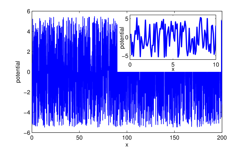
(b)

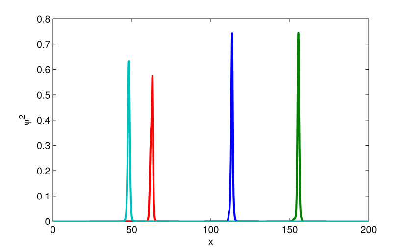
Figure 1: (a) Realization for the white-noise impurity potential on a one-dimensional strip with $L_{\rm s}=2.000$ sites for $L=200$ ($a=0.1$). (b) Occupation probabilities $|\psi_{l,{\rm R}}(n)|^{2}$ for the four lowest-energy eigenstates ($l=1,2,3,4$). At impurity strength $S_{L}=1$, the energies, positions, and standard deviations of the four states are $e=E/{\cal T}=(-1.44,-1.17,-1.10,-0.88)$, $\bar{x}=(113,155,63,48)$, $\Delta x=\sqrt{\bar{x^{2}}-\bar{x}^{2}}=(0.69,0.71,0.79,0.76)$.

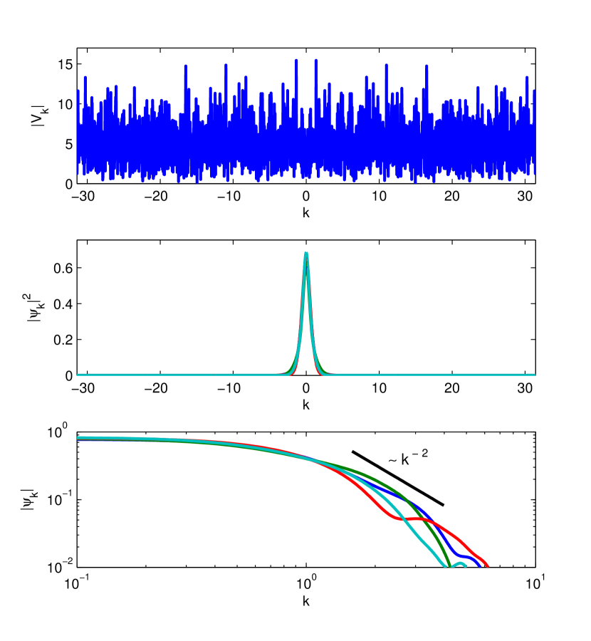
Figure 2: Wave function intensities in momentum space $|\tilde{\psi}_{l,{\rm R}}(k)|^{2}$ for the four states with lowest energy in the potential landscape of Fig. 1, shown in momentum space in the top part of the figure. Note that the Brillouin zone boundaries are at $\pi/a=10\pi$. The bottom part of the figure shows $|\tilde{\psi}_{l,{\rm R}}(k)|$ on a log-log scale.

The amplitude squares $|\tilde{\psi}_{1,{\rm R}}(k)|^{2}$ for the ground state of the Hamiltonian (22) are shown in Fig. 2; the specific realization of the disorder potential is the same as shown in Fig. 1(a). It is seen that a typical low-energy wave packet spreads over a distance $1/\ell_{\rm wp}$ in reciprocal space, and vanishes algebraically for large $k$,

$$\tilde{\psi}(k)\propto\frac{1}{(k\ell_{\rm wp})^{2}}$$ (26)

in one dimension.

This behavior is readily shown to be generic for low-energy states of a one-dimensional Hamiltonian with site-diagonal disorder. We transform the Schrödinger equation (13) in one dimension to reciprocal space,

$$\frac{\hbar^{2}k^{2}}{2m}\tilde{\psi}(k)+\int\frac{{\rm d}q}{2\pi}\tilde{\cal V}_{\rm R}(k-q)\tilde{\psi}(q)=E\tilde{\psi}(k)$$ (27)

with

$$\tilde{\cal V}_{\rm R}(q)=\int_{0}^{L}{\rm d}xe^{-{\rm i}qx}{\cal V}_{\rm R}(x)\;.$$ (28)

From eq. (27), we see that

$$\tilde{\psi}(k)=\frac{1}{\hbar^{2}k^{2}/(2m)-E+{\rm i}\eta}\int\frac{{\rm d}q}{2\pi}\tilde{\cal V}_{\rm R}(k-q)\tilde{\psi}(q)\;,$$ (29)

where $\eta=0^{+}$ to ensure a proper analytic behavior around the pole. Eq. (29) shows that, for small $E$ and large $k$, we reproduce the empirically observed behavior in eq. (26) because, for a representative $\tilde{\cal V}_{\rm R}(k)$, the integral becomes independent of $k$ when $|k|$ becomes large.

III.1.2 Definition of the low-pass filter

Eq. (29) shows that for small $k$ only small $(k-q)$ values contribute to the integral because $k$ and $q$ are both small. Therefore, only small Fourier components of the random potential in eq. (28) are important.

This observation constitutes the basis of the low-pass filter approach. The effective random potential

$$\tilde{W}_{\rm R}(k)=\tilde{\Gamma}(k)\tilde{\cal V}_{\rm R}(k)$$ (30)

leads to the same solution of the Schrödinger equation (27) when we apply the low-pass filter $\tilde{\Gamma}(k)$ that fulfills the conditions

$$\tilde{\Gamma}(k\ll 1/\ell) \approx 1\;,$$ (31)

$$\tilde{\Gamma}(k\gg 1/\ell) \approx \frac{1}{(k\ell)^{2}}\;,$$ (32)

where $\ell$ is a characteristic length scale that remains to be adjusted. Eq. (31) implies that a constant shift in $\bar{\cal V}_{\rm R}(x)$ leads to the same constant shift in $\bar{W}_{\rm R}(x)$.

The effective potential in position space is given by the convolution of the original potential and a weight function,

$$W_{\rm R}(x)=\int_{0}^{L}{\rm d}x^{\prime}\Gamma(x-x^{\prime}){\cal V}_{\rm R}(x^{\prime})$$ (33)

with

$$\Gamma(x)=\int\frac{{\rm d}q}{2\pi}e^{{\rm i}qx}\tilde{\Gamma}(q)\;.$$ (34)

This shows that the oscillations of the white-noise potential are smoothed by the filter function $\Gamma(x)$.

A particularly simple choice for $\tilde{\Gamma}(k)$ that fulfills eq. (32) is a Lorentzian low-pass filter,

$$\tilde{\Gamma}^{\rm L}(k)=\frac{1}{1+(k\ell_{\rm L})^{2}}\;.$$ (35)

In this way, the effective potential in position space is given by the convolution of the original potential and an exponential weight function,

$$W_{\rm R}^{\rm L}(x)=\int_{0}^{L}\frac{{\rm d}x^{\prime}}{2\ell_{\rm L}}e^{-|x-x^{\prime}|/\ell_{\rm L}}{\cal V}_{\rm R}(x^{\prime})\;.$$ (36)

Apparently, the original potential is averaged over the length scale $\ell_{\rm L}$.

III.2 Relation to localization landscape theory

Apart from its apparent simplicity, the Lorentzian low-pass filter offers yet another advantage: it permits to make close contact with the LLT [4, 5, 6, 7].

III.2.1 LLT as a low-pass filter

We note

$$-\frac{{\rm d}^{2}}{{\rm d}x^{2}}W_{\rm R}^{\rm L}(x) = \int\frac{{\rm d}k}{2\pi}\frac{k^{2}}{1+(k\ell_{\rm L})^{2}}e^{{\rm i}kx}\tilde{\cal V}_{\rm R}(k)$$ (38)

$$= \frac{1}{\ell_{\rm L}^{2}}\int\frac{{\rm d}k}{2\pi}e^{{\rm i}kx}\tilde{\cal V}_{\rm R}(k)$$

$$-\frac{1}{\ell_{\rm L}^{2}}\int\frac{{\rm d}k}{2\pi}\frac{1}{1+(k\ell_{\rm L})^{2}}e^{{\rm i}kx}\tilde{\cal V}_{\rm R}(k)$$

$$= \frac{1}{\ell_{\rm L}^{2}}\left({\cal V}_{\rm R}(x)-W_{\rm R}^{\rm L}(x)\right)\;.$$

Therefore, we obtain the defining equation for the effective potential with a Lorentzian low-pass filter in position space

$$\ell_{\rm L}^{2}\frac{{\rm d}^{2}}{{\rm d}x^{2}}W_{\rm R}^{\rm L}(x)+{\cal V}_{\rm R}(x)=W_{\rm R}^{\rm L}(x)\;.$$ (39)

In LLT, the defining equation for the effective potential also only involves the potential itself,

$$-\frac{\hbar^{2}}{2m}\frac{{\rm d}^{2}}{{\rm d}x^{2}}u_{\rm R}(x)+{\cal V}_{\rm R}(x)u_{\rm R}(x)=1$$ (40)

or, with

$$W_{\rm R}(x)=\frac{1}{u_{\rm R}(x)}\;,$$ (41)

we find the LLT equation

$$W_{\rm R}(x)\left(-\frac{\hbar^{2}}{2m}\frac{{\rm d}^{2}}{{\rm d}x^{2}}\right)\left(\frac{1}{W_{\rm R}(x)}\right)+{\cal V}_{\rm R}(x)=W_{\rm R}(x)\;,$$ (42)

which is very similar to the Lorentzian low-pass filter equation (39). We note that, for all practical applications,

$$u_{\rm R}(x)=c+\delta u_{\rm R}(x)$$ (43)

with

$$|\delta u_{\rm R}(x)|\ll c$$ (44)

holds. Therefore, in linear approximation, we have

$$W_{\rm R}(x)=\frac{1}{u_{\rm R}(x)}\approx\frac{1}{c}\left(1-\frac{1}{c}\delta u_{\rm R}(x)\right)$$ (45)

so that

$$\frac{{\rm d}^{2}}{{\rm d}x^{2}}W_{\rm R}(x) \approx -\frac{1}{c^{2}}\frac{{\rm d}^{2}}{{\rm d}x^{2}}\delta u_{\rm R}(x)$$ (46)

$$= -\frac{1}{c^{2}}\frac{{\rm d}^{2}}{{\rm d}x^{2}}u_{\rm R}(x)$$

$$= -\frac{1}{c^{2}}\frac{{\rm d}^{2}}{{\rm d}x^{2}}\left(\frac{1}{W_{\rm R}(x)}\right)\;.$$

When inserted into eq. (42), we find to linear order

$$\frac{1}{c}\left(-\frac{\hbar^{2}}{2m}\frac{{\rm d}^{2}}{{\rm d}x^{2}}\right)\left(-c^{2}W_{\rm R}(x)\right)+{\cal V}_{\rm R}(x)=W_{\rm R}(x)\;,$$ (47)

which reduces to eq. (39) when we identify

$$W_{\rm R}(x)=W_{\rm R}^{\rm L}(x)\;,$$ (48)

$$\frac{1}{c}=\frac{\hbar^{2}}{2m\ell_{\rm L}^{2}}\;.$$ (49)

Note that, since $\delta u_{\rm R}(x)$ is evenly distributed around zero, we have

$$\frac{1}{L}\int_{0}^{L}{\rm d}xW_{\rm R}(x)\approx\frac{1}{L}\int_{0}^{L}{\rm d}x\frac{1}{c}\left(1-\frac{1}{c}\delta u_{\rm R}(x)\right)=\frac{1}{c}\;.$$ (50)

Therefore, the solution of the LLT equation (40) gives $c$ and thus $\ell_{\rm L}$ via eq. (49). It means that the Lorentz-filtered potential is equivalent to the LLT potential when the Lorentz parameter $\ell_{\rm L}$ is determined from eq. (49), where $c^{-1}$ is the mean value of $W_{\rm R}(x)$.

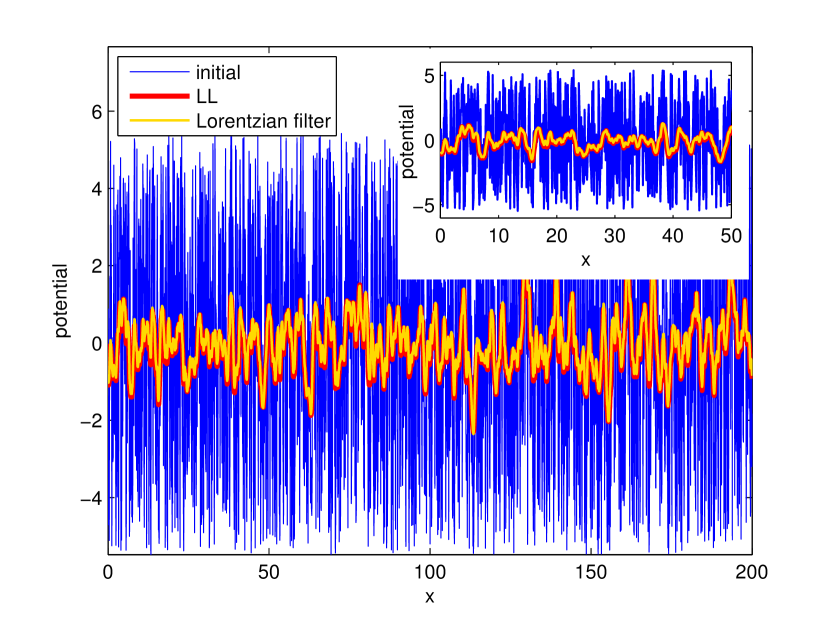
Figure 3: Comparison between LLT and a global Lorentzian filter. The random potential ${\cal V}_{\rm R}(x)$ of Fig. 1(a) is shown as a blue line. The red line is the result of LLT, $W_{\rm R}(x)$, from the solution of Eq. (40). The yellow line shows the potential $W_{\rm R}^{\rm L}(x)$ using a Lorentzian filter, see eq. (36), where $\ell_{\rm L}=0.436\,\ell_{\rm wp}$ is calculated from eqs. (49) and (50).

III.2.2 Visualization

In order to visualize the relation between LLT and the Lorentzian low-pass filter, we re-consider the one-dimensional random potential shown in Fig. 1(a). The LLT requires the solution of the Poisson-type equation (40). The spatial average of the solution $u_{\rm R}(x)$ defines $c$, see eq. (43), which in turn gives the parameter $\ell_{\rm L}$ in the Lorentzian low-pass filter using eq. (49).

In Fig. 3 we compare the effective potentials from LLT and from the Lorentzian low-pass filter. Apparently, the agreement is very good. This one-dimensional example illustrates that LLT and a Lorentzian low-pass filter applied to the white-noise potential lead to equivalent results.

III.2.3 Advantages of the low-pass filer approach

The low-pass filter approach offers several advantages. (i) There are no conceptual problems whereas some gradient terms in the Schrödinger equations are ignored in the motivation of the LLT. (ii) The physical picture of a coarse-grained potential becomes more obvious, see eq. (33). The coarse-graining is permitted because the low-energy wave functions themselves decay algebraically as a function of momentum. (iii) The low-pass filter is not restricted to a Lorentzian shape but the filter functions can be adapted for specific applications.

In the next section we address the improvement of the low-pass filter beyond the Lorentzian shape.

IV Variational approaches as low-pass filters

In the last section, the length-scale parameter $\ell$ in the Lorentzian low-pass filter was fixed by comparison with LLT. In general, however, one would prefer a criterion to optimize not only that length scale but to find the best filter function according to some physical criterion. Variational theories are best suited for this task because they optimize physically motivated cost functions.

The variational approach to the localization problem is far from new. Indeed, almost six decades ago, Halperin and Lax [38] used this approach to determine variationally the average density of states $\rho_{\rm var}(E)$; the result was quantitatively improved by including higher-order corrections [43]. For a Green function approach to white-noise disorder, see Zittartz and Langer [44].

IV.1 Variational theory for localized states

IV.1.1 Ritz variational principle

The Ritz variational principle states that any normalized single-particle wave function $\varphi(\vec{r}\,)$ provides an upper bound to the exact ground-state energy,

$$E_{\rm R}^{\rm var}(\left\{\varphi\right\})=\int{\rm d}^{3}r\varphi^{*}(\vec{r}\,){\cal H}_{\rm R}(\vec{r}\,)\varphi(\vec{r}\,)\geq E_{{\rm R},0}\;,$$ (51)

where $E_{{\rm R},0}$ is the exact ground-state energy for the realization ${\rm R}$. For a given variational state one has to calculate the kinetic energy,

$$t_{\rm var}(\left\{\varphi(\vec{r}\,)\right\})=\int{\rm d}^{3}r\varphi^{*}(\vec{r}\,)T^{\rm op}(\vec{r}\,)\varphi(\vec{r}\,)\;,$$ (52)

and the potential energy,

$$v_{\rm var}(\left\{\varphi(\vec{r}\,)\right\})=\int{\rm d}^{3}r|\varphi(\vec{r}\,)|^{2}{\cal V}_{\rm R}(\vec{r}\,)\;.$$ (53)

To carry out the Ritz variational optimization, the variational states must be further specified.

IV.1.2 Variational localized ground state

For the localization problem, we assume that low-energy states are localized around some $\vec{r}\,{}^{\prime}$ [38],

$$\varphi(\vec{r}\,)\equiv\varphi_{\bm{\alpha}}(\vec{r}\,{}^{\prime}-\vec{r}\,)\;.$$ (54)

Note that the variational state depends on $\vec{r}\,{}^{\prime}$ and further internal parameters $\bm{\alpha}=(\alpha_{1},\alpha_{2},\ldots,)$ that are to be determined variationally. It is assumed that the wave function vanishes fast for $|\vec{r}-\vec{r}\,{}^{\prime}|\gg\ell_{\rm wp}$.

The variational kinetic energy is independent of $\vec{r}\,{}^{\prime}$ because it only induces a constant shift in position space in the wave function. Therefore, the minimization of the variational energy $E_{\rm R}^{\rm var}(\left\{\varphi_{\bm{\alpha}}(\vec{r}\,{}^{\prime})\right\})$ in eq. (51) with respect to $\vec{r}\,{}^{\prime}$ leads to ($i=1,\ldots,d$)

$$\frac{\partial}{\partial r_{i}^{\prime}}\int{\rm d}^{3}r\left|\varphi_{\bm{\alpha}}(\vec{r}\,{}^{\prime}-\vec{r}\,)\right|^{2}{\cal V}_{\rm R}(\vec{r}\,)=0\;.$$ (55)

In other word, the wave function is localized around the minimum of the $\varphi$-potential

$$W_{\rm R}^{\varphi}(\vec{r},\bm{\alpha})=\int{\rm d}^{3}r^{\prime}\left|\varphi_{\bm{\alpha}}(\vec{r}-\vec{r}\,{}^{\prime})\right|^{2}{\cal V}_{\rm R}(\vec{r}\,{}^{\prime})\;.$$ (56)

Note that the variational state and energy remain to be optimized with respect to the variational parameters $\bm{\alpha}$ in $\varphi$, i.e., the total variational energy

$$E_{\rm R}^{\varphi}(\vec{r},\bm{\alpha})=t_{\rm R}^{\varphi}(\bm{\alpha})+W_{\rm R}^{\varphi}(\vec{r},\bm{\alpha})$$ (57)

remains to be optimized with respect to $\bm{\alpha}$. In this way, position, shape, and energy of the ground state of the Hamiltonian ${\cal H}_{\rm R}(\vec{r}\,)$ are determined variationally.

Apparently, we may interpret $W_{\rm R}^{\varphi}(\vec{r},\bm{\alpha})$ at the optimized values as the effective potential landscape in the vicinity of $\vec{r}\,{}^{\prime}$ where the particle is localized in the ground state.

IV.2 Local low-pass filters

IV.2.1 Concept

In general, the Ritz variational principle is restricted to find an upper bound for the ground-state energy. For the localization problem, it can be used to detect many more energetically low-lying states because these are typically separated by distances that are large compared to their width in position space, $\ell_{\rm hop}\gg\ell_{\rm wp}$. Thus, we may find the positions of several low-energy states by using the following strategy.

• For fixed parameter set $\bm{\alpha}^{(1)}\equiv\bm{a}$ define the global low-pass filter

  $$\Gamma_{\bm{a}}(\vec{r}\,{}^{\prime}-\vec{r}\,)=\left|\varphi_{\bm{a}}(\vec{r}\,{}^{\prime}-\vec{r}\,)\right|^{2}\;.$$ (58)

  A first estimate for the particle positions is given by the minima of

  $$W_{\rm R}^{\varphi}(\vec{r},\bm{a})=\int{\rm d}^{3}r^{\prime}\Gamma_{\bm{a}}(\vec{r}\,{}^{\prime}-\vec{r}\,){\cal V}_{\rm R}(\vec{r}\,{}^{\prime})\;,$$ (59)

  see eq. (56). The resulting minima are denoted by $\vec{s}_{j}^{\,(1)}$, $j=1,2,\ldots\;$.

• Iterate to convergence the following steps: For given $\vec{s}_{j}^{\,(n)}$, optimize the variational parameters to find a new set $\bm{\alpha}^{(n+1)}$; for this new set of parameters, optimize the position to obtain $\vec{s}_{j}^{\,(n+1)}$.

As a result, we obtain the variational landscape in the vicinity of the minima $\vec{s}_{j}^{\;{\rm opt}}$ as

$$W_{\rm R}(\vec{r},\bm{\alpha}^{\rm opt})=\int{\rm d}^{3}r^{\prime}\left|\varphi_{\bm{\alpha}^{\rm opt}}(\vec{r}-\vec{r}\,{}^{\prime})\right|^{2}{\cal V}_{\rm R}(\vec{r}\,{}^{\prime})$$ (60)

in the regions $|\vec{r}-\vec{s}_{j}^{\;{\rm opt}}|\lesssim\ell_{\rm wp}$.

IV.2.2 Gauss filter

To illustrate the concept of a local low-pass filter, we apply a Gauss filter to the one-dimensional localization problem,

$$\varphi(x^{\prime}-x,\omega)=\left(\frac{m\omega}{\pi\hbar}\right)^{1/4}\exp\left(-\frac{m\omega(x^{\prime}-x)^{2}}{2\hbar}\right)\;,$$ (61)

where $x^{\prime}$ is the position of the wave packet and $\omega$ characterizes its width $\ell_{\rm G}=\sqrt{\hbar^{2}/(2m\hbar\omega)}$, so that we must optimize only one internal parameter, $\alpha_{1}\equiv\omega$. The variational energy reads

$$E_{\rm R}^{\rm var}(x^{\prime},\omega)=\frac{\hbar\omega}{4}+\int_{-\infty}^{\infty}\frac{{\rm d}k}{2\pi}e^{{\rm i}kx^{\prime}}\exp\left(-\frac{(k\ell_{\rm G})^{2}}{2}\right)\tilde{\cal V}_{\rm R}(k)\;,$$ (62)

using Fourier transformation, where we used that the variational kinetic energy $t_{\rm G}=\hbar\omega/4$ for a Gaussian wave function.

The integral in eq. (62) can be calculated very efficiently by Fast-Fourier-Transformation so that the minima of the variational energy can be found from a scan of the two-dimensional $(x^{\prime},\omega)$ space. In Fig. 4 we show the results for the first ten localized states. It is seen that the positions of the lowest-lying states are very well reproduced, and that the variational energies provide a reasonable estimate for the exact values.

The energy estimate can be improved systematically by using a sum of several Gaussians with different widths as variational state. We shall not pursue this approach here.

IV.2.3 Gauss-Lorentz filter

The effective potential deviates from its quadratic shape when $|x-x^{\prime}|\gtrsim\ell_{\rm G}$. It approaches the shape of a potential barrier with constant height so that the wave function decays exponentially, as is also seen in reciprocal space in eq. (32). Therefore, it is preferable to combine a Gaussian and a Lorentzian filter so that the variational energy is determined from the minima of the function

$$E_{\rm R}^{\rm var} = t_{\rm GL}+v_{\rm GL}\;,$$

$$v_{\rm GL} = \int_{-\infty}^{\infty}\frac{{\rm d}k}{2\pi}\frac{e^{{\rm i}kx^{\prime}}}{1+\eta(k\ell_{\rm G})^{2}}e^{-\frac{(1-\eta)(k\ell_{\rm G})^{2}}{2}}\tilde{\cal V}_{\rm R}(k)\;,$$

$$\varphi(x) = \left[\int_{-\infty}^{\infty}\frac{{\rm d}k}{2\pi}\frac{e^{{\rm i}kx}}{1+\eta(k\ell_{\rm G})^{2}}e^{-\frac{(1-\eta)(k\ell_{\rm G})^{2}}{2}}\right]^{1/2}$$ (63)

$$t_{\rm GL} = \frac{\hbar^{2}}{2m}\int_{-\infty}^{\infty}{\rm d}x\left[\varphi^{\prime}(x)\right]^{2}\;,$$

where we abbreviated $E_{\rm R}^{\rm var}(x^{\prime},\omega,\eta)\equiv E_{\rm R}^{\rm var}$. The optimal values for $\eta_{j}$ for the localized states at $x_{j}^{\prime}$ are found to lie in the range $0.6\leq\eta_{j}\leq 0.8$.

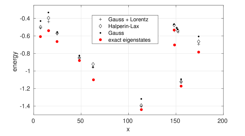
Figure 4: Positions of the ten lowest-lying localized states and their energies (red points) for the random potential of Fig. 1. The black dots, crosses, and diamonds indicate the positions and energies for Gauss, Gauss-Lorentz, and Halperin-Lax filters, respectively.

In Fig. 4 we also include the results from the Gauss-Lorentz filter. Since we enlarge the variational space, the energies from the Gauss-Lorentz states are closer to the exact results. Note that a combination of Gaussian and Lorentzian variational states is similar in spirit to the application of the LLT to a random potential with Gaussian averaging, see eq. (21).

IV.2.4 Halperin-Lax filter

Halperin and Lax used a variational approach to calculate the density of states deep in the band tails [38]. Their approach provides the functional form that best fits the typical low-energy localized state. In three dimensions, the Halperin-Lax state $f(\vec{r}\,)$ is obtained from the solution of the third-order equation

$$T^{\rm op}(\vec{r}\,)f(\vec{r}\,)-\mu\frac{{\cal V}^{2}(\ell_{\rm pf})^{3}}{12}[f(\vec{r}\,)]^{3}=Ef(\vec{r}\,)$$ (64)

for the case of Gaussian white noise. This equation is also obtained from the method of optimal fluctuations by Baranovskii and Efros [39].

We introduce the length unit $\ell_{\rm wp}$, $\vec{r}=\ell_{\rm wp}\vec{x}$, and the energy unit ${\cal T}$ so that $e=E/{\cal T}$ and $\bar{\cal V}={\cal V}/{\cal T}$. Moreover, we set $\mu=\tilde{\mu}/{\cal T}$, and $f(\vec{r}\,)=F(\vec{x}\,)/\sqrt{\ell_{\rm pf}^{3}}$. Then, the dimension-less Halperin-Lax equation reads

$$-\sum_{i=1}^{3}\frac{\partial^{2}F(\vec{x}\,)}{\partial x_{i}^{2}}-\tilde{\mu}S_{L}[F(\vec{x}\,)]^{3}=eF(\vec{x}\,)\;,$$ (65)

where

$$S_{L}=\frac{\bar{\cal V}^{2}}{12}\left(\frac{\ell_{\rm pf}}{\ell_{\rm wp}}\right)^{3}$$ (66)

is the dimensionless impurity interaction strength in three dimensions.

In one dimension, the dimensionless Halperin-Lax equation reads

$$-F^{\prime\prime}(x)-\tilde{\mu}S_{L}[F(x)]^{3}=eF(x)$$ (67)

with the normalized solution [38]

$$F(x)=\sqrt{\frac{\kappa}{2}}\frac{1}{\cosh(\kappa x)}\;,$$ (68)

where the decay length $\ell_{\rm HL}=1/\kappa$ depends on the energy $e$,

$$\kappa\equiv\kappa(e)=\sqrt{-e}=\frac{1}{\ell_{\rm HL}}$$ (69)

and $\tilde{\mu}=4\kappa/S_{L}$.

For low energies, the resulting variational density of states $\rho_{\rm var}(E)$ in one dimension agrees in its functional form with the exact solution [45, 46, 47] up to a factor $1/\sqrt{5}$ [38]. Extensions to variational states that include perturbative corrections to the form (68) permit to obtain the exact prefactor to the low-energy density of states [43, 44].

Apparently, the Halperin-Lax wave function $F(x)$ in eq. (68) interpolates between Gaussian behavior for small distances and exponential behavior for large distances using only a single parameter. The results for the Halperin-Lax filter where we replace $\varphi(x)$ in eqs. (51)–(53) by $F(x)$ are also included in Fig. 4. They are better than those obtained from the Gauss filter and comparably good as those obtained from the Gauss-Lorentz filter.

The Halperin-Lax filter offers the following advantages. First, it does not find too many states, i.e., as seen in Fig. 4, there is one Halperin-Lax state for every exact localized state whereas Gauss and Gauss-Lorentz find an additional state in the region of $x\approx 150$. We observed this behavior also for other realizations ${\rm R}$. Second, the Halperin-Lax wave function gives good variational energies using only a single variational parameter for its decay length, $\ell_{{\rm HL},j}=1/\kappa_{j}$ for the $j$th minimum. Third, the Halperin-Lax wave function provides the optimal form for localized low-energy states in a statistical sense. Therefore, we come to the conclusion that the Halperin-Lax filter is the most appropriate one-parameter local low-pass filter.

IV.3 Halperin-Lax global low-pass filter

A global low-pass filter includes a finite set of length scales that are independent of the realization ${\rm R}$. To determine their values, we should optimize the agreement with physical quantities that are obtained by averaging over many realizations, e.g., the density of states $\rho(E)$ in eq. (14). Below we shall focus on the construction of a global Halperin-Lax filter in one dimension.

IV.3.1 Motivation

Eq. (69) suggests that the width of the wave function increases as a function of energy. As expected, the lowest-lying states have the smallest spread in position space. For a given realization ${\rm R}$, the surrounding of the potential well also plays an important role. Therefore, the relation between between binding energy and wave-function width is not always so simple as suggested in eq. (69). This is shown in Fig. 5, where we display the relation between the lowest exact energies $e_{l}$ and the corresponding standard deviations $\ell_{{\rm HL},j}$ of the wave packets for $\ell_{\rm HL}$ for 26.000 realizations ${\rm R}$ of systems with $L_{s}=2.000$ and $L=200$ for $S_{L}=1$.

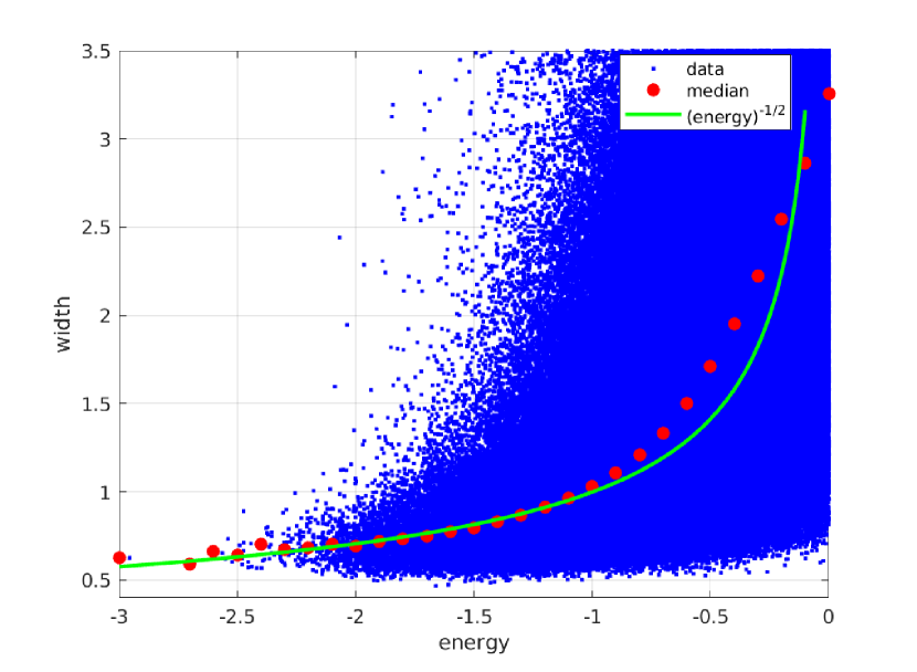
Figure 5: Relation between the exact energies for the lowest-lying localized states $e_{j}$ and the corresponding standard deviations $\ell_{{\rm HL},j}$ of the wave packets in the Halperin-Lax wave function in one dimension, see eq. (68). Also shown is the median of the data (red dots) and the Halperin-Lax relation $\ell_{\rm HL}(e)=1/\sqrt{-e}$, see eq. (69).

As seen from Fig. 5, the median follows the relation (69) but there is considerable spread in the values $\ell_{\rm HL}$. Nevertheless, since the typical energy values are of the order $S_{L}^{2/3}{\cal T}$, the full variety of local variational wave functions can be approximated by a prototypical wave function when $\ell_{\rm HL}/(\ell_{\rm wp}S_{L}^{1/3})$ lies in the fairly small interval $I_{\ell_{\rm HL}}=[0.8,1.2]$. Therefore, it is permissible to replace the set of local Halperin-Lax low-pass filters by a global Halperin-Lax low-pass filter,

$$\Gamma^{\rm HL}(y)=\frac{1}{2\ell_{\rm HL}}\frac{1}{\cosh^{2}(y/\ell_{\rm HL})}\;.$$ (70)

The corresponding potential landscape becomes

$$W_{\rm R}^{\rm HL}(x)=\int{\rm d}x^{\prime}\Gamma^{\rm HL}(x-x^{\prime}){\cal V}_{\rm R}(x^{\prime})$$ (71)

for a given realization ${\rm R}$ of the random white-noise potential. The remaining task is to determine the ‘best’ value for $\ell_{\rm HL}$.

IV.3.2 Tail optimization

One strategy suggested by Fig. 5 is to optimize the states in the low-energy tail. To optimize the tail states, one should choose

$$\frac{\ell_{\rm HL}^{\rm tail}S_{L}^{1/3}}{\ell_{\rm wp}}=0.8$$ (72)

in eq. (70). Since there are exponentially few states in the tails, this is not the best strategy to describe the system at elevated temperatures. Therefore, we shall not elaborate this choice any further.

IV.3.3 Classical state counting

In Fig. 6 (upper part) we reproduce the Lorentzian landscape from LLT with $\ell_{\rm L}=0.436\,\ell_{\rm wp}$ for the realization of the random potential shown in Fig. 1(a), as already shown in Fig. 3. Here, we add the exact positions and energies of the 30 lowest-lying states. It is seen that there is a reasonable overall agreement between the positions and depth of the minima in the LLT landscape and the exact results. However, the potential is still noisy and some minima do not support an exact eigenstate.

The Halperin-Lax potential landscape shown in the lower part of Fig. 6 is much smoother because $\ell_{\rm HL}=1.2\,\ell_{\rm wp}$ at $S_{L}=1$ is almost three times larger than $\ell_{\rm L}$. More importantly, all minima for energies below $e=-0.5$ correspond to a localized state in the exact solution of the Schrödinger equation. If we choose $\ell_{\rm L}=1.2\,\ell_{\rm wp}$ for the Lorentzian filter, the corresponding effective potential becomes less noisy but there still are quite a number of local minima that do not correspond to an exact bound state. The reason for this behavior is the cusp at $x=x^{\prime}$ in the Lorentzian filter, see eq. (36). The smooth Halperin-Lax filter in eq. (70) avoids these artificial potential fluctuations.

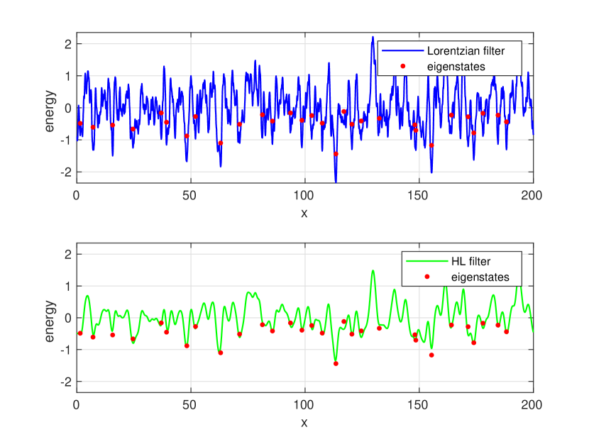
Figure 6: (a) Effective potential $W_{\rm R}^{\rm L}(x)$ for a global Lorentzian low-pass filter for $\ell_{\rm L}=0.436\,\ell_{\rm wp}$, see eq. (36) and Fig. 3. (b) Effective potential $W_{\rm R}^{\rm HL}(x)$ for a global Halperin-Lax low-pass filter for $\ell_{\rm HL}=1.2\,\ell_{\rm wp}$ ($S_{L}=1$), see eq. (71). Also shown in both figures are the exact positions and energies of the 30 states lowest in energy.

As seen from Fig. 6, the Halperin-Lax filter not only reproduces the spatial positions of the localized states but also their energy with very good accuracy. This indicates that a classical counting of states will provide a reasonable estimate for the integrated particle density $N(e)$ below the energy $e=E/{\cal T}$ that is known exactly for random white-noise potential in one dimension [45, 46, 47],

$$N(e) = \int_{-\infty}^{e}{\rm d}\epsilon\rho(\epsilon)\;,$$

$$= \frac{1}{2^{1/3}\pi^{2}}\left[[\mathop{\rm Ai}(-2^{2/3}e)]^{2}+[\mathop{\rm Bi}(-2^{2/3}e)]^{2}\right]^{-1},$$

where $\mathop{\rm Ai}(x)$ and $\mathop{\rm Bi}(x)$ are the Airy functions of the first and second kind,

$$\mathop{\rm Ai}(x) = {\frac{1}{\pi}}\int\limits_{0}^{\infty}{\rm d}t\cos\left({\frac{t^{3}}{3}}+xt\right)\;,$$ (74)

$$\mathop{\rm Bi}(x) = {\frac{1}{\pi}}\int\limits_{0}^{\infty}\,{\rm d}t\left[\exp\left(-{\frac{t^{3}}{3}}+xt\right)+\sin\left({\frac{t^{3}}{3}}+xt\right)\right]\;.$$

We concisely re-derive the result (IV.3.3) in appendix A. Furthermore, in the same appendix A we derive the expression for the energy-dependent localization length $a(e)$ in the white-noise one-dimensional potential.

Treating $W_{\rm R}^{\rm HL}(x)$ as a classical potential, we denote the minima at position $x_{i}$ with energy $e_{i}$ by the set $M_{\rm R}^{\rm HL}=\{(x_{i,{\rm R}},e_{i,{\rm R}})\}$. Then, the number of states up energy $e$ is given by classical counting

$$N_{\rm cl}^{\rm HL}(e) = \langle N_{\rm cl,R}(e)\rangle\;,$$

$$N_{\rm cl,R}(e) = \frac{1}{L}\sum_{M_{\rm R}^{\rm HL}}\Theta(e-e_{i,{\rm R}})\;,$$ (75)

where $\Theta(x)$ is the Heaviside step function. $N_{\rm cl,R}(e)$ simply counts the minima with energy up to $e$ in the realization ${\rm R}$ of the Halperin-Lax potential.

The exact result $N(e)$ in one dimension (IV.3.3) and the result from classical counting of minima (75) are compared in Fig. 7. It is seen that the classical counting works very well deep in the tail, $e\lesssim-1$, and still gives reasonable results up to the band edge, $e_{\rm be}=0$. The results are best for $\ell_{\rm HL}=1.2\,\ell_{\rm wp}$ and slightly poorer when we choose $\ell_{\rm HL}=\ell_{\rm wp}$.

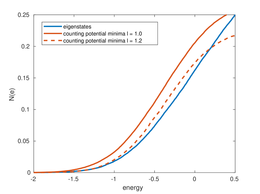
Figure 7: Exact result for the integrated particle density up to energy $e$, $N(e)$ from eq. (IV.3.3), in comparison with the classical counting of minima, $N_{\rm cl}(e)$ from eq. (75), for the Halperin-Lax potential for $\ell_{\rm HL}=1.2\,\ell_{\rm wp}$ (dashed line) and $\ell_{\rm HL}=1.0\,\ell_{\rm wp}$ (full line) ($S_{L}=1$). Averages are taken over 1.000 realizations ${\rm R}$.

The success of the classical counting of minima shows that the Halperin-Lax potential ought to be viewed as a suitable effective potential for classical particles.

IV.3.4 Semi-classical state counting

In Ref. [4], Arnold et al. proposed to use the LLT potential in the semi-classical Weyl expression [48] to approximate the integrated particle density $N(e)$. For particles in a potential landscape $W_{\rm R}(x)$ in one dimension it reads [4]

$$N_{\rm W}(E) = \frac{1}{L}\frac{\sqrt{2m}}{\pi\hbar}\langle\int{\rm d}r\sqrt{E-W_{\rm R}(r)}\Theta\left(E-W_{\rm R}(r)\right)\rangle\;,$$

$$N_{\rm W}(e) = \frac{1}{L}\frac{1}{\pi}\langle\int{\rm d}x\sqrt{e-\bar{W}_{\rm R}(x)}\Theta\left(e-\bar{W}_{\rm R}(x)\right)\rangle\;,$$ (76)

where the second line gives the dimensionless expression where energies are measured in units of ${\cal T}$.

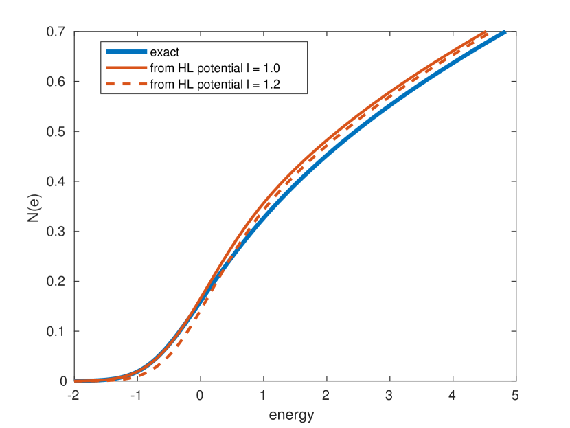
Figure 8: Integrated particle density $N(e)$ up to energy $e=E/{\cal T}$ in a one-dimensional random white-noise potential. The exact result (IV.3.3) is compared with the semi-classical state counting using eqs. (78) and (79) for a Halperin-Lax filter with $\ell_{\rm HL}=1.2\,\ell_{\rm wp}$ (dashed line) and with $\ell_{\rm HL}=1.0\,\ell_{\rm wp}$ (full line) ($S_{L}=1$), averaged over 1.000 configurations with 2.000 sites for $L=200$.

Obviously, one should not use $W_{\rm R}^{\rm HL}(x)$ in eq. (76) because the Weyl formula starts from the assumption that the total energy is the sum of the kinetic energy and the potential energy. For given $\ell_{\rm HL}$, the kinetic energy of the variational state is a constant,

$$\bar{T}_{0}=\frac{1}{{\cal T}}\frac{\hbar^{2}}{2m}\int{\rm d}r\left[F^{\prime}(r)\right]^{2}=\frac{1}{3}\left(\frac{\ell_{\rm wp}}{\ell_{\rm HL}}\right)^{2}$$ (77)

in units of ${\cal T}$. Therefore, we must shift the classical potential $\bar{W}_{\rm R}(x)$ by $\bar{T}_{0}$,

$$\widetilde{W}_{\rm R}(x)=\bar{W}_{\rm R}(x)-\bar{T}_{0}\;,$$ (78)

and we employ

$$N_{\rm scl}(e)=\frac{1}{L}\frac{1}{\pi}\langle\int{\rm d}x\sqrt{e-\widetilde{W}_{\rm R}(x)}\Theta\left(e-\widetilde{W}_{\rm R}(x)\right)\rangle$$ (79)

for an appropriate semi-classical approximation of the number of states up to energy $e$.

In Fig. 8 we compare the exact result for the integrated particle density up to energy $e$, eq. (IV.3.3), with the (shifted) semi-classical expression (79) for the Halperin-Lax potential at $\ell_{\rm HL}=1.2\,\ell_{\rm wp}$ and $\ell_{\rm HL}=1.0\,\ell_{\rm wp}$, obtained from an average over 1.000 configurations for $L_{\rm s}=2.000$ sites for system length $L=200$ ($S_{L}=1$). The comparison shows that the semi-classical approximation faithfully reproduces the exact result up to the band edge $e_{\rm be}=0$, and remains reasonable even beyond. The results for $\ell_{\rm HL}=1.2\,\ell_{\rm wp}$ are slightly poorer than those for $\ell_{\rm HL}=1.0\,\ell_{\rm wp}$ but still astonishingly good. Thus, the shifted Halperin-Lax potential provides a sound basis for a semi-classical description of particles in a localization landscape.

V Conclusions

In this work, we discussed a number of approaches to deeply localized states in disordered systems. Therefore, after we put our work into perspective, we summarize the proposed strategies. We close our presentation with a short outlook.

V.1 Perspective

In disordered systems, the potential experienced by the carriers fluctuates on an atomic length scale, $\ell_{\rm pf}=1\,\hbox{\AA}$. In contrast, the localized low-energy states spread over a much larger length scale, namely $\ell_{\rm wp}\approx 10\ell_{\rm pf}\gg\ell_{\rm pf}$. In addition, states with comparable energy are well separated in space, $\ell_{\rm hop}\gg\ell_{\rm wp}$. Therefore, it is advisable to take advantage of the separation of length and energy scales for localized states in the band tails.

When charge carriers move between these localized states, the microscopic length scale $\ell_{\rm pf}$ becomes irrelevant, and only a coarse-grained potential landscape remains to be considered. It is the goal of the localization landscape theory (LLT) [4, 5, 6, 7], in its application to electronic states in disordered media, to derive systematically useful landscape $W_{\rm R}(\vec{r}\,)$ for a given realization ${\rm R}$ of the fluctuating potential ${\cal V}_{\rm R}(\vec{r}\,)$. Landscapes are useful if they reliably reproduce the spatial positions and energies of the low-lying localized states.

The LLT application to the Schrödinger equation is based on the solution of eq. (1). The corresponding LLT potentials have been applied successfully to a variety of disordered systems. In this work, we first showed that the LLT corresponds to a global Lorentzian low-pass filter where the solution of eq. (1) fixes the single length-scale $\ell_{\rm L}$. This observation cleared the way to investigate the full range of decay lengths and a broader class of low-pass filters to extend and improve the LLT-inspired methods systematically. The resulting strategies are summarized as follows.

V.2 Strategies

For low temperatures, the low-energy states deep in the band tails are of particular importance. There are several ways to determine their physical properties, each of which having its merits and disadvantages.

• Exact results are obtained from the solution of the Schrödinger equation. From there, expectation values for physical quantities are calculated exactly for a given configuration of the disorder potential, and averages over many realizations are required.

  This approach is very time-consuming and not feasible in three dimensions, especially when the calculations are part of a self-consistent loop, i.e., when they need to be repeated a large number of times.

• The localization landscape theory (LLT) provides a far less time-consuming alternative [4, 5, 6, 7] because it provides a smooth potential $W_{\rm R}(\vec{r}\,)$ that can be used for (semi-)classical considerations.

  However, the LLT still requires the solution of eq. (1) for each realization. Moreover, the LLT foundations and limits for its applicability remained unclear.

• The structure of the low-energy wave functions of the Hamiltonian justifies the application of a low-pass filter to the potential. In particular, application of the LLT corresponds to a Lorentzian low-pass filter, see eq. (36) for the definition of the landscape $W_{\rm R}^{\rm L}(\vec{r}\,)$.

  The value for the decay length $\ell_{\rm L}$ in the Lorentzian low-pass filter can be estimated from the solution of the LLT eq. (1) for a single realization. Alternatively, one may take $\ell_{\rm L}$ as the width of the ground-state wave packet of the Hamiltonian for some configuration ${\rm R}$, or simply set $\ell_{\rm L}=\ell_{\rm wp}$. For an expression of $\ell_{\rm wp}$ as a function of the system parameters, see appendix B. In this way, the solution of eq. (1) becomes superfluous.

• When individual localized states are required for a given realization of the random potential, local low-pass filters (Gauss, Gauss-Lorentz, Halperin-Lax) can be applied. These methods are very efficient because expectation values can be calculated using Fast-Fourier-Transformation techniques, and the optimized states provide a fairly accurate variational description of deeply localized states.

• The best global low-pass filter is not provided by the Lorentzian filter. The optimal filter in a statistical sense is obtained from the solution of the Halperin-Lax equation (64); the latter equation is not limited to random white-noise potentials.

  Using the Halperin-Lax low-pass filter as global filter leads to the Halperin-Lax potential landscape $W_{\rm R}^{\rm HL}(\vec{r}\,)$, see eqs. (70) and (71) for one spatial dimension and a random white-noise potential. The Halperin-Lax potential can be viewed as potential landscape for classical particles. A classical state counting reproduces the exact integrated particle density $N(e)$ at low energies surprisingly well.

• When the kinetic energy is taken into account, the shifted Halperin-Lax potential $W_{\rm R}^{\rm HL}(\vec{r}\,)-T_{0}$, see eq. (78), can be used for a semi-classical description of particles in a random potential. The Weyl approximation for the density of states using $W_{\rm R}^{\rm HL}(\vec{r}\,)-T_{0}$ reproduces the exact result for the integrated particle density $N(e)$ in one dimension with very good accuracy.

V.3 Outlook

In this work, we derived the concept of a global Halperin-Lax low-pass filter for the localization landscape theory, and successfully applied it to particles in a one-dimensional random white-noise potential. It remains to be tested that the size of a typical wave packet can be used as characteristic length for the Halperin-Lax filter also in two and three dimensions.

The Halperin-Lax filter can be found from the solution of a integro-differential equation that reduces to a non-linear differential equation for the case of white noise. Therefore, the localization landscape obtained with a Halperin-Lax filter can readily be applied to random potentials with correlations. In this case, more than one length scale $\ell_{\rm wp}$ might be necessary to parameterize the low-pass filter appropriately.

For transport, not only the typical distance $\ell_{\rm hop}$ between energetically low-lying states is important but also the typical potential landscape between them determines the tunnel probabilities between those states. Further studies are necessary to clarify whether or not the localization landscape with Halperin-Lax filter is useful to describe hopping transport at finite temperatures.

The main focus of the LLT in solids is not the single-particle density of states but rather the particle density $n(\vec{r},T)$ that depends on space $\vec{r}$ and temperature $T$. In our subsequent paper [40] we calculate $n(\vec{r},T)$ without solving the Schrödinger equation. Thereby, the full quantum-mechanical problem is reduced to the quasi-classical description of $n(\vec{r},T)$ in a temperature-dependent effective potential $W(\vec{r}\,,T)$. Our approximate results for $n(\vec{r},T)$ and for the carrier mobility at elevated temperatures favorably compare with those from the exact solution of the Schrödinger equation [40]. The temperature-dependence of $W(\vec{r}\,,T)$ leads to superior results in comparison with the temperature-independent LLT landscape $W(\vec{r})$.

Appendix A Random white-noise potential in one dimension

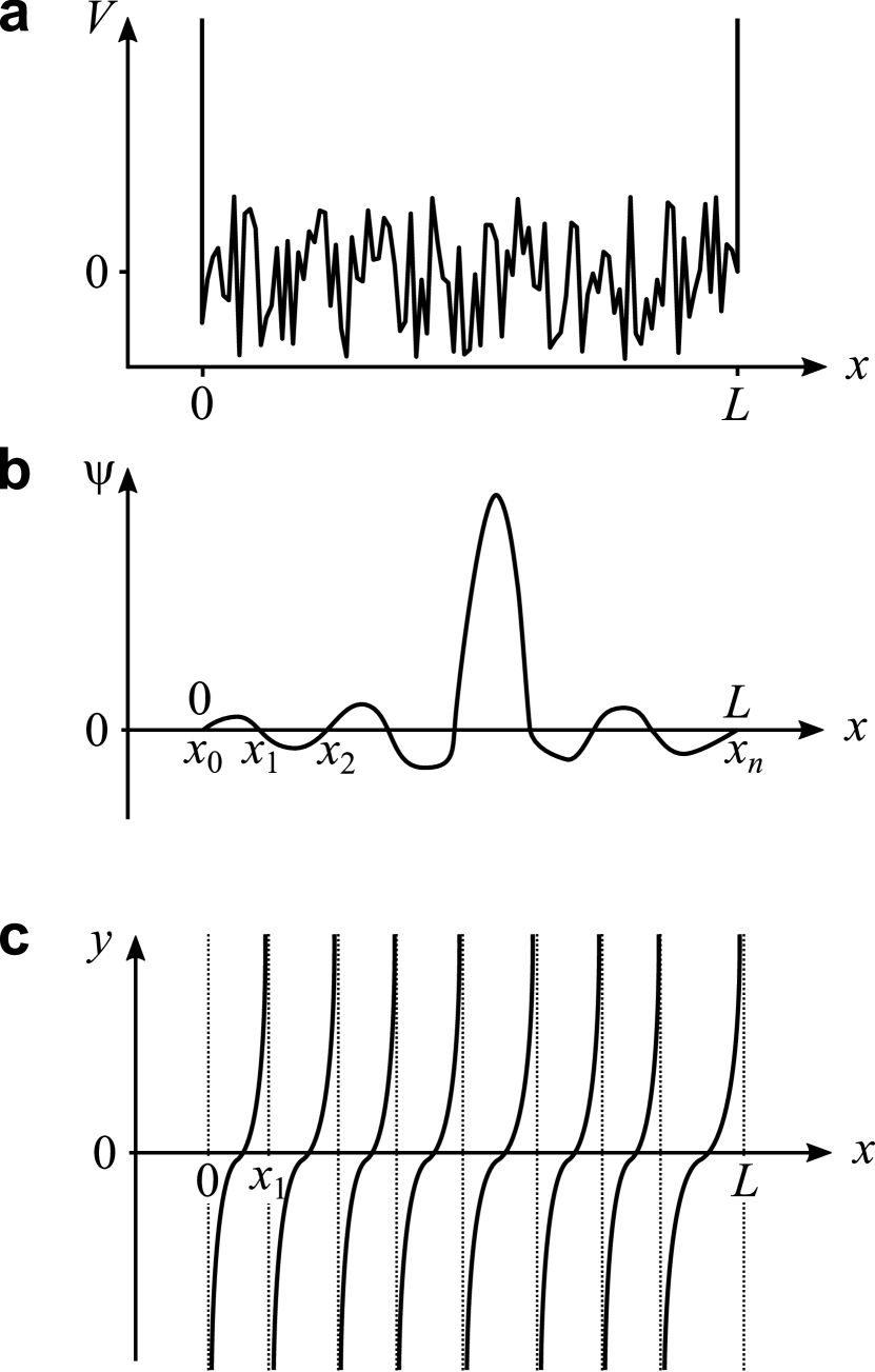
Figure 9: Localized state in a one-dimensional random white-noise potential. (a) sketch of potential $V(x)$; (b) wave function $\psi(x)$ that corresponds to the $n$th eigenstate whose energy is approximately equal to $e$; (c) function $y(x)=-\psi^{\prime}(x)/\psi(x)$. The particle is confined between infinite walls at $x=0$ and $x=L$. The zeros of the wave function are labeled by $x_{1}$, $x_{2}$, et cetera.

A.1 Density of states

The one-dimensional Hamiltonian eq. (6) gives rise to the Schrödinger equation

$$-\psi^{\prime\prime}(x)+V(x)\psi(x)=e\psi(x)\;,$$ (80)

where $V(x)$ is a normalized white-noise potential,

$$\langle V(x)\rangle=0\;,\quad\langle V(x_{1})V(x_{2})\rangle=\delta(x_{1}-x_{2})\;.$$ (81)

We consider a particle confined within a range $x\in[0,L]$, see Fig. 9(a), implying open boundary conditions

$$\psi(0)=\psi(L)=0\;.$$ (82)

In the limit $L\to\infty$, the energy spectrum of the particle becomes continuous. Therefore, for a very large length $L$, any given energy $e$ can be approximated by some energy level in this system, i.e., some solution of the Schrödinger equation (80). Let $n(e)$ denote the number of states up to this energy level, counting from below, so that

$$N(e)=\frac{n(e)}{L}\;.$$ (83)

The aim of this Appendix is to derive the expression (IV.3.3) for $N(e)$ in the limit of $L\to\infty$.

According to the oscillatory theorem, the wave function $\psi(x)$ that corresponds to the $n$th energy level has $n+1$ zeros, $x_{0}=0$, $x_{1}$, $\ldots$, $x_{n}=L$, see Fig. 9(b). Let us consider the function

$$y(x)=-\frac{\psi^{\prime}(x)}{\psi(x)}\;.$$ (84)

A schematic plot of this function is shown in Fig. 9(c).

Taking the derivative $y^{\prime}(x)$ in eq. (84) and expressing $\psi^{\prime\prime}$ via eq. (80), one can obtain a first-order differential equation for the function $y(x)$,

$$y^{\prime}(x)=y(x)^{2}+e-V(x)\;.$$ (85)

For a further analysis of eq. (85), it is convenient to interpret the variable $x$ as ‘time’. Then, the function $y(x)$ can be understood as describing the movement of some point along the ‘coordinate’ $y$ in ‘time’ $x$. According to eq. (85), this movement is a combination of drift with velocity

$$v(y)=y^{2}+e$$ (86)

and a diffusion due to a Langevin force introduced by the white-noise term in eq. (85) [49].

We determine the diffusion coefficient $D$ in the corresponding Fokker–Planck equation from the statistics of the random white-noise potential $V(x)$. To this end, we ignore the drift term, and consider the diffusive equation of motion with only the white-noise term present, $y^{\prime}=-V(x)$. Its solution is $y(x)=y(0)-\int_{0}^{x}V(x_{1})\,{\rm d}x_{1}$. Therefore, the mean square of the displacement along $y$ during the ‘time’ $x$ is

$$\left\langle[y(x)-y(0)]^{2}\right\rangle = \left\langle\int_{0}^{x}V(x_{1})\,{\rm d}x_{1}\int_{0}^{x}V(x_{2})\,{\rm d}x_{2}\right\rangle$$ (87)

$$= \int_{0}^{x}{\rm d}x_{1}\int_{0}^{x}{\rm d}x_{2}\left\langle V(x_{1})V(x_{2})\right\rangle$$

$$= x\;,$$

where we used the white-noise correlation function (81). By definition, the left-hand side of eq. (87) is equal to $2Dx$ [49]. Hence, $2Dx=x$, i.e.,

$$D=\frac{1}{2}$$ (88)

holds for the diffusion coefficient.

In the Fokker–Planck picture, the motion of a singular ‘point’ described by eq. (85) can be recast into the form of a flow of the distribution of such points. Let us introduce the distribution function $f(y)$ that correspond to uniformly distributed coordinate $x$ in the range $0\leq x\leq L$, i.e., $f(y){\rm d}y$ is the probability that $y(x)$ falls into the range $[y,y+{\rm d}y]$ when $x$ is distributed uniformly,

$$f(y){\rm d}y=\frac{1}{L}{\rm d}x\;.$$ (89)

Since the function $f(y)$ describes the ‘time’-averaged distribution, it must remain unchanged under the motion governed by eq. (85). Therefore, the continuity equation dictates that

$$\frac{{\rm d}j(y)}{{\rm d}y}=0\;,$$ (90)

where $j(y)$ is the flow of points due to drift and diffusion,

$$j(y)=v(y)f(y)-D\frac{{\rm d}f(y)}{{\rm d}y}\;.$$ (91)

Substituting the drift velocity $v(y)$ and the diffusion coefficient $D$ form eqs. (86) and (88), one obtains a differential equation for distribution function $f(y)$ [49],

$$(y^{2}+e)f(y)-\frac{1}{2}\frac{{\rm d}f(y)}{{\rm d}y}=c\;,$$ (92)

where $c$ is a constant that is determined from the boundary conditions below.

To find the unique solution $f(y)$ of this equation we employ the boundary conditions at $y\to\pm\infty$. It is evident from eq. (84) that large $|y|$ correspond to small $\psi(x)$, i.e., to the neighborhoods of the zeros $x_{0},\ldots,x_{n}$ of the wave function $\psi(x)$. Keeping only the linear term in the Taylor series around $r$th zero, $x_{r}$, we obtain

$$y(x)=-\frac{\psi^{\prime}(x)}{\psi(x)}\approx-\frac{\psi^{\prime}(x_{r})}{(x-x_{r})\,\psi^{\prime}(x_{r})}=\frac{1}{x_{r}-x}\;.$$ (93)

Using the equations (89) and (93), we see that $f(y)\approx 1/(Ly^{2})$ for large $y^{2}$. This result must be multiplied by the number of zeros $n$ because each of them gives a contribution to $f(y)$. We recall that $n(e)=LN(e)$ from eq. (83) and obtain the boundary conditions

$$f(y)\to\frac{N(e)}{y^{2}}\;\text{for}\;|y|\to\infty\;.$$ (94)

Inserting this expression into eq. (92) leads to the value of the constant $c$,

$$c=N(e)\;.$$ (95)

It is worth noting that the ‘flow’ $c$ has a meaning of the inverse average distance between zeros of the wave functions, i.e., the inverse average ‘time’ of the motion from $y=-\infty$ to $y=+\infty$.

The first-order differential equation (92) with $c=N(e)$ and boundary conditions (94) is readily solved by the method of undetermined coefficients,

$$f(y) = 2N(e)\exp\left(\frac{2y^{3}}{3}+2ey\right)$$ (96)

$$\times\int_{y}^{+\infty}\exp\left(-\frac{2u^{3}}{3}-2eu\right){\rm d}u\;.$$

Finally, $N(e)$ can be calculated by inserting (96) into the normalization condition for the distribution $f(y)$,

$$\int_{-\infty}^{+\infty}f(y){\rm d}y=1\;.$$ (97)

To evaluate eq. (97), we must perform the integrations over $u$ and $y$. It is convenient to make the substitution $u=y+t$ in eq. (96) after which the integral over the new variable $t$ acquires constant limits, $0\leq t<\infty$. Switching the order of integrations gives rise to a Gaussian integral over $y$. After integration over $y$, the normalization condition (97) takes the form

$$\sqrt{2\pi}N(e)\int_{0}^{\infty}\frac{{\rm d}t}{\sqrt{t}}\exp\left(-\frac{t^{3}}{6}-2et\right)=1\;.$$ (98)

The remaining integral can be expressed using Airy functions $\mathop{\rm Ai}(x)$ and $\mathop{\rm Bi}(x)$ of the first and the second kind [50, p. 32]. This leads to expression (IV.3.3) for the integrated particle density $N(e)$.

The result (IV.3.3) is valid for a certain set of unit lengths and energies in which the Schrödinger equation has the dimensionless form of eq. (80), and the statistics of the potential is also dimensionless, see eq. (81). However, it is easy to rewrite eq. (IV.3.3) in arbitrary units. To do this, it is enough to insert a factor of dimension (energy)^-1 into the arguments of the Airy functions, and to multiply the whole expression by a factor of dimension (length)^-1. These dimension factors must be products of appropriate powers of the quantities $\hbar$, $2m$, and $S$, where $S$ is defined by eq. (5). The resulting expression reads

$$N(E) = \frac{1}{\pi^{2}}\sqrt[3]{\frac{2Sm^{2}}{\hbar^{4}}}\Biggl{\{}\left[\mathop{\rm Ai}\left(-\sqrt[3]{\frac{2\hbar^{2}}{mS^{2}}}\;E\right)\right]^{2}$$ (99)

$$+\left[\mathop{\rm Bi}\left(-\sqrt[3]{\frac{2\hbar^{2}}{mS^{2}}}\;E\right)\right]^{2}\Biggr{\}}^{-1}.$$

Here, all quantities are expressed in SI units.

A.2 Localization length

In one dimension, all electron eigenstates are Anderson-localized. A wave function $\psi(x)$ of such an eigenstate has exponential tails at $x\to\pm\infty$:

$$\psi(x)\simeq\exp(-|x|/a),$$ (100)

where coordinate $x$ is counted from the center of the eigenstate, and $a$ is the localization length.

Here we calculate $a$ as a function of the electron energy in a random white-noise potential.

We consider the left tail ($x<0$), where $\ln\psi(x)\approx(x/a)+const$. The quantity $1/a$ is therefore equal to

$$\frac{1}{a}=\lim_{x\to-\infty}\frac{\ln[\psi(0)]-\ln[\psi(x)]}{0-x}=\left\langle\frac{\mathrm{d}\ln\psi(x)}{\mathrm{d}x}\right\rangle_{x\in(-\infty,0)}.$$ (101)

In terms of the function $y(x)$ determined by eq. (84),

$$\frac{1}{a}=-\langle y\rangle=-\int_{-\infty}^{+\infty}y\,f(y)\,\mathrm{d}y,$$ (102)

where $f(y)$ is the distribution function of $y$ determined by eq. (96). Substituting this expression into eq. (102), one can calculate the localization length $a$. A convenient way for this calculation is to make the substitution $u=y+t$, then integrate over $y$ from $-\infty$ to $+\infty$, and finally integrate over $t$ from 0 to $+\infty$. The result reads:

$$\frac{1}{a}=-\frac{\pi^{2}}{2^{5/3}}\,N(e)\,\frac{\mathrm{d}\left[[\mathop{\rm Ai}(-2^{2/3}e)]^{2}+[\mathop{\rm Bi}(-2^{2/3}e)]^{2}\right]}{\mathrm{d}e}\,,$$ (103)

where $e$ is the dimensionless energy, and $N(e)$ is the integrated DOS. The combination of Airy functions $\mathop{\rm Ai}$ and $\mathop{\rm Bi}$ in the latter equation is related to the integrated DOS by eq. (IV.3.3):

$$[\mathop{\rm Ai}(-2^{2/3}e)]^{2}+[\mathop{\rm Bi}(-2^{2/3}e)]^{2}=\frac{1}{2^{1/3}\pi^{2}N(e)}\,.$$ (104)

Combining equations (103) and (104), one can get the (dimensionless) localization length $a$ as a function of the dimensionless energy $e$:

$$a(e)=4\left[\frac{\mathrm{d}\ln N(e)}{\mathrm{d}e}\right]^{-1},$$ (105)

where $N(e)$ is given by eq. (IV.3.3).

One can rewrite this expression in physical (SI) units by replacing $\mathrm{d}/\mathrm{d}e$ with ${\cal T}(\mathrm{d}/\mathrm{d}E)$ and multiplying the right-hand side by $\ell_{\rm wp}$, where $\cal T$ and $\ell_{\rm wp}$ are given by eq. (117), and $E$ is the energy in physical units:

$$a(E)=\frac{2\hbar^{2}}{mS}\left[\frac{\mathrm{d}\ln N(E)}{\mathrm{d}E}\right]^{-1}.$$ (106)

Function $N(E)$ here is given by eq. (99).

Let us consider the limiting cases. At high energies, $E\to+\infty$, the integrated DOS $N(E)$ is proportional to $\sqrt{E}$, just as in a one-dimensional conduction band in the absence of disorder. Hence, $\mathrm{d}\ln N(E)/\mathrm{d}E=1/2E$, and

$$a(E)=\frac{4\hbar^{2}E}{mS}\,.$$ (107)

At low energies $E\to-\infty$, i. e. deeply in the band tail, one can omit $\mathop{\rm Ai}$ in eq. (99), and use asymptotic formula $\mathop{\rm Bi}(x)\approx\exp(\frac{2}{3}x^{3/2})/(\sqrt{\pi}x^{1/4})$, which gives $N(E)\sim\exp\left[\frac{4}{3}\sqrt{\frac{2\hbar^{2}}{mS^{2}}}(-E)^{3/2}\right]$. Substitution of this estimate into eq. (106) yields

$$a(E)=\frac{\hbar}{\sqrt{-2mE}}=\frac{1}{k}\,.$$ (108)

It is well-known [51] that the localization length $a(E)$ in 1D can be expressed via the integrated density of states $N(E)$ in an integral form. It follows from the results of Ref. [51] that

$$\frac{1}{a(E)}=\int_{-\infty}^{+\infty}\frac{N(E^{\prime})-N_{0}(E^{\prime})}{E-E^{\prime}}\,\mathrm{d}E^{\prime}+\kappa_{0}(E),$$ (109)

where the Cauchy principal value of the integral is assumed, $N_{0}(E)$ is the free-particle integrated density of states,

$$N_{0}(E)=\begin{cases}\;\;\;\;0&\text{ if }E\leq 0,\\ \frac{\sqrt{2mE}}{\pi\hbar}&\text{ if }E\geq 0,\end{cases}$$ (110)

and $\kappa_{0}(E)$ is the inverse localization length of a particle in zero barrier potential,

$$\kappa_{0}(E)=\begin{cases}\frac{\sqrt{-2mE}}{\hbar}&\text{ if }E\leq 0,\\ \;\;\;\;\;0&\text{ if }E\geq 0.\end{cases}$$ (111)

We have checked numerically that both expressions for localization length $a(E)$, eq. (106) and eq. (109), yield identical results for the white-noise integrated density of states $N(E)$ given by eq. (99).

The advantage of our eq. (106) is that it provides an expression for the localization length in a closed form, rather than in a form of an integral. On the other hand, this expression is valid only in the case of a white-noise random potential. For other 1D potentials, the more complicated eq. (109) should be used.

Appendix B Energy and length scales

In Section II.1, we considered features of a particle in a random potential such as the typical width of the wave packet $\ell_{\rm wp}$, the typical kinetic energy of a localized state $\cal T$, and the strength of the potential $S$. The latter two quantities are defined in eqs. (4) and (5), respectively. Then, we introduced a dimensionless representation, in which $\ell_{\rm wp}$ and $\cal T$ are used as units of length and energy. The aim of this appendix is to fix the values of $\ell_{\rm wp}$ and $\cal T$ so that the strength of the potential becomes equal to unity in dimensionless units.

To achieve this goal, we present a dimensionless version of eq. (5) that defines the dimensionless disorder strength $S_{L}$,

$$\langle\bar{\cal V}_{\rm R}(\vec{x}\,)\bar{\cal V}_{\rm R}(\vec{x}\,{}^{\prime})\rangle_{\rm R}=S_{L}\delta\left(\vec{x}-\vec{x}\,{}^{\prime}\right)\;,$$ (112)

where $\vec{x}=\vec{r}/\ell_{\rm wp}$ and $\bar{\cal V}_{\rm R}={\cal V}_{\rm R}/{\cal T}$ are scaled coordinates and potentials. We divide both sides of eq. (112) by the corresponding sides of eq. (5), and take into account that $\delta\left(\vec{x}-\vec{x}\,{}^{\prime}\right)=\delta\left[(\vec{r}-\vec{r}\,{}^{\prime})/\ell_{\rm wp}\right]=\ell_{\rm wp}^{d}\delta\left(\vec{r}-\vec{r}\,{}^{\prime}\right)$ and obtain

$$\frac{1}{{\cal T}^{2}}=\frac{S_{L}}{S}\,\ell_{\rm wp}^{d}$$ (113)

in $d$ dimensions. Substituting $\cal T$ from eq. (4), we express the dimensionless strength of the disorder potential as

$$S_{L}=\frac{S}{{\cal T}^{2}\ell_{\rm wp}^{d}}=S\frac{(2m)^{2}\ell_{\rm wp}^{4-d}}{\hbar^{4}}\;.$$ (114)

Now we assume $S_{L}=1$ which yields

$$\ell_{\rm wp}=\left(\frac{\hbar^{4}}{4m^{2}S}\right)^{1/(4-d)}$$ (115)

for the width of the wave packet and

$${\cal T}=\frac{\hbar^{2}}{2m\ell_{\rm wp}^{2}}=\left(\frac{2m}{\hbar^{2}}\right)^{d/(4-d)}S^{2/(4-d)}$$ (116)

for the typical kinetic energy of a localized state. In one dimension ($d=1$),

$$\ell_{\rm wp}=\frac{\hbar^{4/3}}{(2m)^{2/3}S^{1/3}}\quad,\quad{\cal T}=\frac{(2m)^{1/3}S^{2/3}}{\hbar^{2/3}}\;.$$ (117)

Note that the expressions (115)–(117) are unique combinations of $[2m]=\text{M}$, $[\hbar]=\text{M}\text{L}^{2}/\text{T}$ and $[S]=\text{E}^{2}\text{L}^{d}=\text{M}^{2}\text{L}^{4+d}/\text{T}^{4}$ that possess the correct dimensions.

References

- Baranovski [2006] S. D. Baranovski, ed., Charge Transport in Disordered Solids with Applications in Electronics (John Wiley and Sons, Ltd, Chichester, 2006).
- Masenda et al. [2021] H. Masenda, L. M. Schneider, M. Adel Aly, S. J. Machchhar, A. Usman, K. Meerholz, F. Gebhard, S. D. Baranovskii, and M. Koch, Energy scaling of compositional disorder in ternary transition-metal dichalcogenide monolayers, Adv. Electron. Mater. 7, 2100196 (2021).
- Weisbuch et al. [2021] C. Weisbuch, S. Nakamura, Y.-R. Wu, and J. S. Speck, Disorder effects in nitride semiconductors: impact on fundamental and device properties, Nanophotonics 10, 3 (2021).
- Arnold et al. [2016] D. N. Arnold, G. David, D. Jerison, S. Mayboroda, and M. Filoche, Effective confining potential of quantum states in disordered media, Phys. Rev. Lett. 116, 056602 (2016).
- Filoche et al. [2017] M. Filoche, M. Piccardo, Y.-R. Wu, C.-K. Li, C. Weisbuch, and S. Mayboroda, Localization Landscape Theory of disorder in semiconductors. I. Theory and modeling, Phys. Rev. B 95, 144204 (2017).
- Piccardo et al. [2017] M. Piccardo, C.-K. Li, Y.-R. Wu, J. S. Speck, B. Bonef, R. M. Farrell, M. Filoche, L. Martinelli, J. Peretti, and C. Weisbuch, Localization Landscape Theory of disorder in semiconductors. II. Urbach tails of disordered quantum well layers, Phys. Rev. B 95, 144205 (2017).
- Li et al. [2017] C.-K. Li, M. Piccardo, L.-S. Lu, S. Mayboroda, L. Martinelli, J. Peretti, J. S. Speck, C. Weisbuch, M. Filoche, and Y.-R. Wu, Localization Landscape Theory of disorder in semiconductors. III. Application to carrier transport and recombination in light emitting diodes, Phys. Rev. B 95, 144206 (2017).
- Montoya et al. [2021] J. A. G. Montoya, A. Tibaldi, C. De Santi, M. Meneghini, M. Goano, and F. Bertazzi, Nonequilibrium Green’s function modeling of trap-assisted tunneling in InxGa1-xN/ GaN light-emitting diodes, Phys. Rev. Appl. 16, 044023 (2021).
- Tibaldi et al. [2021] A. Tibaldi, J. A. G. Montoya, M. Vallone, M. Goano, E. Bellotti, and F. Bertazzi, Modeling infrared superlattice photodetectors: from nonequilibrium Green’s functions to quantum-corrected drift diffusion, Phys. Rev. Appl. 16, 044024 (2021).
- Liu et al. [2019] W. Liu, G. Rossbach, A. Avramescu, T. Schimpke, H.-J. Lugauer, M. Strassburg, C. Mounir, U. T. Schwarz, B. Deveaud, and G. Jacopin, Impact of alloy disorder on Auger recombination in single InGaN/GaN core-shell microrods, Phys. Rev. B 100, 235301 (2019).
- Chen et al. [2018] H.-H. Chen, J. S. Speck, C. Weisbuch, and Y.-R. Wu, Three-dimensional simulation on the transport and quantum efficiency of UVC-LEDs with random alloy fluctuations, Appl. Phys. Lett. 113, 153504 (2018).
- Tsai et al. [2020] T.-Y. Tsai, K. Michalczewski, P. Martyniuk, C.-H. Wu, and Y.-R. Wu, Application of Localization Landscape Theory and the kp model for direct modeling of carrier transport in a type-II superlattice InAs/InAsSb photoconductor system, J. Appl. Phys. 127, 033104 (2020).
- Di Vito et al. [2020] A. Di Vito, A. Pecchia, A. Di Carlo, and M. Auf der Maur, Simulating random alloy effects in III-nitride light emitting diodes, J. Appl. Phys. 128, 041102 (2020).
- Chaudhuri et al. [2021] D. Chaudhuri, M. O’Donovan, T. Streckenbach, O. Marquardt, P. Farrell, S. K. Patra, T. Koprucki, and S. Schulz, Multiscale simulations of the electronic structure of III-nitride quantum wells with varied indium content: Connecting atomistic and continuum-based models, J. Appl. Phys. 129, 073104 (2021).
- Chow et al. [2020] Y. C. Chow, C. Lee, M. S. Wong, Y.-R. Wu, S. Nakamura, S. P. DenBaars, J. E. Bowers, and J. S. Speck, Dependence of carrier escape lifetimes on quantum barrier thickness in InGaN/GaN multiple quantum well photodetectors, Opt. Express 28, 23796 (2020).
- Shamailov et al. [2021] S. S. Shamailov, D. J. Brown, T. A. Haase, and M. D. Hoogerland, Computing the eigenstate localisation length at very low energies from Localisation Landscape Theory, SciPost Phys. Core 4, 017 (2021).
- Zhan et al. [2021] J. Zhan, Z. Chen, C. Li, Y. Chen, J. Nie, Z. Pan, C. Deng, X. Xi, F. Jiao, X. Kang, S. Li, Q. Wang, T. Yu, Y. Tong, G. Zhang, and B. Shen, Investigation on many-body effects in micro-LEDs under ultra-high injection levels, Opt. Express 29, 13219 (2021).
- Shen et al. [2021] H.-T. Shen, C. Weisbuch, J. S. Speck, and Y.-R. Wu, Three-dimensional modeling of minority-carrier lateral diffusion length including random alloy fluctuations in (,) and (,) single quantum wells, Phys. Rev. Appl. 16, 024054 (2021).
- Shen et al. [2022] H.-T. Shen, Y.-C. Chang, and Y.-R. Wu, Analysis of light-emission polarization ratio in deep-ultraviolet light-emitting diodes by considering random alloy fluctuations with the 3d k·p method, physica status solidi (RRL) – Rapid Research Letters 16, 2100498 (2022).
- Bertazzi et al. [2020] F. Bertazzi, A. Tibaldi, M. Goano, J. A. G. Montoya, and E. Bellotti, Nonequilibrium Green’s function modeling of type-II superlattice detectors and its connection to semiclassical approaches, Phys. Rev. Appl. 14, 014083 (2020).
- O’Donovan et al. [2021] M. O’Donovan, D. Chaudhuri, T. Streckenbach, P. Farrell, S. Schulz, and T. Koprucki, From atomistic tight-binding theory to macroscale drift–diffusion: Multiscale modeling and numerical simulation of uni-polar charge transport in (In,Ga)N devices with random fluctuations, J. Appl. Phys. 130, 065702 (2021).
- O’Donovan et al. [2022] M. O’Donovan, P. Farrell, T. Streckenbach, T. Koprucki, and S. Schulz, Multiscale simulations of uni-polar hole transport in (In,Ga)N quantum well systems, Optical and Quantum Electronics 54, 405 (2022).
- Chaudhuri et al. [2020] D. Chaudhuri, J. C. Kelleher, M. R. O’Brien, E. P. O’Reilly, and S. Schulz, Electronic structure of semiconductor nanostructures: A modified Localization Landscape Theory, Phys. Rev. B 101, 035430 (2020).
- Balasubramanian et al. [2020] S. Balasubramanian, Y. Liao, and V. Galitski, Many-body localization landscape, Phys. Rev. B 101, 014201 (2020).
- Steinerberger [2017] S. Steinerberger, Localization of quantum states and landscape functions, Proc. Amer. Math. Soc. 145, 2895 (2017).
- Steinerberger [2021] S. Steinerberger, Regularized potentials of Schrödinger operators and a local landscape function, Communications in Partial Differential Equations 46, 1262 (2021).
- Lu et al. [2022] J. Lu, C. Murphey, and S. Steinerberger, Fast localization of eigenfunctions via smoothed potentials, Journal of Scientific Computing 90, 38 (2022).
- Altmann and Peterseim [2019] R. Altmann and D. Peterseim, Localized computation of eigenstates of random Schrödinger operators, SIAM Journal on Scientific Computing 41, B1211 (2019).
- Altmann et al. [2020] R. Altmann, P. Henning, and D. Peterseim, Quantitative Anderson localization of Schrödinger eigenstates under disorder potentials, Mathematical Models and Methods in Applied Sciences 30, 917 (2020).
- Jia et al. [2022] C. Jia, Z. Liu, and Z. Zhang, Some mathematical aspects of Anderson localization: boundary effect, multimodality, and bifurcation, Communications in Theoretical Physics 74, 115005 (2022).
- Harrell II and Maltsev [2020] E. M. Harrell II and A. V. Maltsev, Localization and landscape functions on quantum graphs, Trans. Amer. Math. Soc. 373, 1701 (2020).
- Chenn et al. [2022] I. Chenn, W. Wang, and S. Zhang, Approximating the ground state eigenvalue via the effective potential, Nonlinearity 35, 3004 (2022).
- Grubišić et al. [2021] L. Grubišić, M. Hajba, and D. Lacmanović, Deep neural network model for approximating eigenmodes localized by a confining potential, Entropy 23, 10.3390/e23010095 (2021).
- Lemut et al. [2020] G. Lemut, M. J. Pacholski, O. Ovdat, A. Grabsch, J. Tworzydło, and C. W. J. Beenakker, Localization landscape for Dirac fermions, Phys. Rev. B 101, 081405(R) (2020).
- Herviou and Bardarson [2020] L. Herviou and J. H. Bardarson, localization landscape for highly excited states, Phys. Rev. B 101, 220201(R) (2020).
- Comtet and Texier [2020] A. Comtet and C. Texier, Comment on “Effective confining potential of quantum states in disordered media”, Phys. Rev. Lett. 124, 219701 (2020).
- Römer et al. [2021] F. Römer, M. Guttmann, T. Wernicke, M. Kneissl, and B. Witzigmann, Effect of inhomogeneous broadening in ultraviolet III-nitride light-emitting diodes, Materials 14, 10.3390/ma14247890 (2021).
- Halperin and Lax [1966] B. I. Halperin and M. Lax, Impurity-band tails in the high-density limit. I. Minimum counting methods, Phys. Rev. 148, 722 (1966).
- Baranovskii and Efros [1978] S. D. Baranovskii and A. L. Efros, Band edge smearing in solid solutions, Sov. Phys. Semicond. 12, 1328 (1978).
- Nenashev et al. [2023] A. V. Nenashev, S. D. Baranovskii, K. Meerholz, and F. Gebhard, Quantum states in disordered media. II. Spatial charge carrier distribution, Phys. Rev. B (2023).
- Ashcroft and Mermin [1976] N. Ashcroft and D. Mermin, Solid State Physics (Holt, Rinehart and Winston, Philadelphia, 1976).
- Shklovskii and Efros [1984] B. I. Shklovskii and A. L. Efros, Electronic Properties of Doped Semiconductors (Springer, Berlin, 1984).
- Halperin and Lax [1967] B. I. Halperin and M. Lax, Impurity-band tails in the high-density limit. II. Higher order corrections, Phys. Rev. 153, 802 (1967).
- Zittartz and Langer [1966] J. Zittartz and J. S. Langer, Theory of bound states in a random potential, Phys. Rev. 148, 741 (1966).
- Frisch and Lloyd [1960] H. L. Frisch and S. P. Lloyd, Electron levels in a one-dimensional random lattice, Phys. Rev. 120, 1175 (1960).
- Halperin [1965] B. I. Halperin, Green’s functions for a particle in a one-dimensional random potential, Phys. Rev. 139, A104 (1965).
- Lax [1966] M. Lax, Classical noise IV: Langevin methods, Rev. Mod. Phys. 38, 541 (1966).
- Weyl [1912] H. Weyl, Das asymptotische Verteilungsgesetz der Eigenwerte linearer partieller Differentialgleichungen (mit einer Anwendung auf die Theorie der Hohlraumstrahlung), Mathematische Annalen 71, 441 (1912).
- van Kampen [2007] N. van Kampen, Stochastic Processes in Physics and Chemstry, 3rd ed. (Elsevier, Amsterdam, 2007).
- Muldoon [1977] M. E. Muldoon, Higher monotonicity properties of certain Sturm-Liouville functions. V, Proc. Roy. Soc. Edinburgh Sect. A 77, 23 (1977).
- Thouless [1972] D. J. Thouless, A relation between the density of states and range of localization for one dimensional random systems, J. Phys. C: Solid State Physics 5, 77 (1972).