Abstract

In this paper we try to understand the Island formula from a purely quantum information perspective. We propose that the island phase is a property of the quantum state and the Hilbert space where the state is embedded in. More explicitly, when certain constraints are imposed in a quantum system by projecting out certain states in the Hilbert space, such that for all the states remaining in the reduced Hilbert space, there exists a mapping from the state of the subset $\mathcal{R}$ to the state of another subset $I$, which we call a coding relation. We call such a system self-encoded. In a self-encoded system the way we compute the reduced density matrix changes essentially, which results in a new island formula to calculate the entanglement entropy. Furthermore, we propose that, the island formula in gravitational theories, which is proposed to rescue the unitarity in the process of black hole evaporation, should be a special application of this new island formula. The combination of these two island formulas indicates that the effective theory of a gravity is a self-encoded theory with the Hilbert spaces vastly reduced.

 

Contents

1. 1 Introduction
2. 2 Reduction in two-spins system
   1. 2.1 Self-encoded quantum systems
   2. 2.2 The simplest case of two spins
3. 3 Islands and Hilbert space reduction
   1. 3.1 Islands from more generic reductions
   2. 3.2 Self-encoding property from gravitational renormalization?
   3. 3.3 Requirements for the Hilbert space reductions
   4. 3.4 Islands beyond spatial regions
   5. 3.5 The resolution of the Mathur/AMPS paradox in a toy model
4. 4 A simulation of Hilbert space reduction via Weyl transformation
   1. 4.1 Finite cutoff from Weyl transformation in CFT₂
   2. 4.2 Weyl transformed CFT vs AdS/BCFT
5. 5 Discussion
6. A The cutoff spheres and their common tangent
7. B Islands in the lab?

 

1 Introduction

The information paradox for evaporating black holes [1, 2, 3, 4, 5] is one of the most important mysteries in our understanding of nature. It was expected that finding a solution to the information paradox could lead us to a window to understand the quantum theory of gravity. The AdS/CFT correspondence [6, 7, 8], which relates asymptotically AdS gravity theories with certain conformal field theories with large central charges and strong coupling, provides us a framework to study the quantum aspects of gravity through its field theory dual. This is called the holographic property of gravity and is believed to be a general property for gravity theories, which strongly indicates that the quantum theory of gravity should be manifestly unitary. Nevertheless, a concrete understanding of how the information is preserved during the black hole evaporation is not obvious at all. A major breakthrough along this line is the study of quantum entanglement structure of the field theories and their corresponding dual gravity counterparts. In the context of AdS/CFT, the Ryu-Takayanagi (RT) formula [9, 10, 11] relates the entanglement entropy of any subregion in the boundary CFT to certain co-dimension two minimal (extremal) surfaces in the bulk which are homologous to the corresponding boundary subregion. This formula was further refined to the quantum extremal surface (QES) formula which included the quantum correction from bulk fields [12, 13].

The authors of Ref. [19, 20, 21, 22] applied the QES prescription to compute the entanglement entropy of the radiation from an evaporating black hole after the Page time. Remarkably they found that, the result deviates from Hawking’s calculations and is consistent with unitary evolution. These computations further inspired the proposal of the so-called “island formula” [23, 24, 25, 26, 27], which is claimed to be the formula to compute the entanglement entropy in quantum systems coupled to gravity. The island formula has been extensively studied in configurations consisting of a system on a fixed spacetime background (or non-gravitational system) and a system with dynamical gravity. The two systems are glued together at some surface with transparent boundary conditions for matter fields, and hence the radiation from a black hole in the gravitating region can enter the non-gravitational system freely. In this setup the non-gravitational system plays the role of a reservoir that absorbs the Hawking radiation.

When we calculate the entanglement entropy for certain subregion $\mathcal{R}$ in an effective field theory, for example the radiation that is stored in the non-gravitational reservoir, the standard way is to calculate the von Neumann entropy for the quantum fields in $\mathcal{R}$, as was done by Hawking [1],

$$Hawking^{\prime}s~{}calculation:\qquad S(\rho_{\mathcal{R}})=S(\tilde{\rho}_{\mathcal{R}})\,.$$ (1)

Here $\rho_{\mathcal{R}}$ is the reduced density matrix for any region $\mathcal{R}$ in the ”full quantum theory” (including quantum gravity effects for which we do not have the exact description), while the tilde reduced density matrix $\tilde{\rho}_{\mathcal{A}}$ for the degrees of freedom settled on the region $\mathcal{A}$ is defined by tracing out all the degrees of freedom in the complement $\bar{\mathcal{A}}$ in the semi-classical effective theory description. It is taken for granted that, the degrees of freedom at different sites in the Cauchy surface where the effective theory lives should be independent from each other, as they are space-like separated. Then Hawking’s calculation follows a standard definition of the reduced density matrix in quantum information.

Nevertheless, unitarity requires the entanglement entropy for the Hawking radiation to follow the Page curve [2], which deviates from Hawking’s calculation after the Page time. Also the Mathur/AMPS puzzle [4, 5] arises after the Page time near the horizon, where the effective field theory description is believed to be valid by that time near the horizon. It seems that, something very important happens to the effective field theory after the Page time, which is hidden to us.

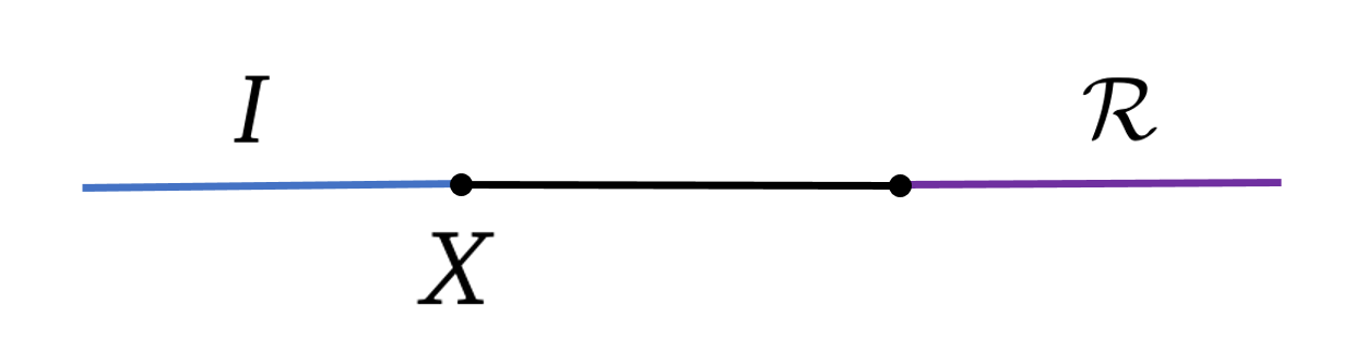
Figure 1: Schematics of the quantum extremal surface $X$ for a subregion $\mathcal{R}$ in a quantum field theory coupled to semiclassical gravity. The region $I$ in the gravitational background bounded by $X$ is the island corresponding to the region $\mathcal{R}$ in non-gravitational background.

The island formula claims that, when calculating $S_{\mathcal{R}}$ we should not only consider the degrees of freedom inside $\mathcal{R}$, but also certain degrees of freedom in the gravitational region $I$ outside $\mathcal{R}$, called the entanglement island, whose boundary is the quantum extremal surface $X$. More explicitly, $S_{\mathcal{R}}$ is still calculated in the semi-classic effective theory description, but with a different formula given by [23, 20, 24, 25, 26]:

$$Island~{}formula~{}I:\qquad S(\rho_{\mathcal{R}})=\text{min}\left\{\text{ext}_{X}\left[\frac{Area(X)}{4G}+S_{bulk}(\tilde{\rho}_{I\cup\mathcal{R}})\right]\right\}\,,$$ (2)

where $X$ is the co-dimension two surface that extrimizes $S({\rho_{\mathcal{R}}})$ calculated by (2), and $I$ represents the region bounded by $X$ and is termed “island” since it is usually disconnected from the region $\mathcal{R}$. See Fig.1 for a simple configuration of the island phase. Note that, according to [12] the sum of the two terms on the right hand side of (2) is indeed the von Neumann entropy of the reduced density matrix computed by tracing out the degrees of freedom outside $\mathcal{R}\cup I$, which we denote as $\tilde{\rho}_{\mathcal{R}\cup I}$, in the large $c$ limit. The area term is the gravitational contribution while the second term computes the non-gravitational contribution, i.e. the bulk entanglement entropy in the semi-classic effective field theory. Between the island formula (2) and the usual formula (1), one should choose the one that gives the smaller entanglement entropy. Remarkably, after the Page time there are configurations where (2) applies, thus entanglement islands emerges just after the Page time. The new formula to calculate entanglement entropy implies that in island phases the following equality may be questioned,

$$\rho_{\mathcal{R}}=\tilde{\rho}_{\mathcal{R}}\qquad??$$ (3)

The doubly holographic set-up discussed in [23] provides a special framework to explain the origin of the island formula. In this scenario, the quantum field theory describing the Hawking radiation is assumed to be holographic. The corresponding bulk dual gravitational theory (Fig.2(a)) has a lower dimensional effective description (Fig.2(b)) in terms of the radiation bath coupled to semi-classical gravity where the island prescription applies. Furthermore, when the AdS₂ gravity part is again holograhically dual to a (0+1)-dimensional quantum dot, we arrived at the third picture of the same configuration, which is called the fundamental description (Fig.2(c)). In the doubly holographic framework, the entanglement entropy of a subsystem in the radiation bath is computed through the usual (H)RT formula [9, 18] which is equivalent to the island prescription in the lower dimensional effective description (Fig.2). The doubly holographic setup naturally encapsulates the idea of the island in the black hole interior being encoded in the entanglement wedge of the radiation. Moreover, in a more general set-up without assuming holography, the island formula has been derived via gravitational path integrals where wormholes are allowed to exist as new saddles (called the replica wormholes) when calculating the partition function on the replica manifold [26, 27]. For a subset of relevant works that may be related to this paper, see [28, 29, 30, 31, 32, 33, 34, 35, 36, 37, 38, 39, 40, 41, 42] and also [43, 44, 45, 46, 47, 48, 49]. Also, see [50, 51] and the references therein for a detailed review on this topic.

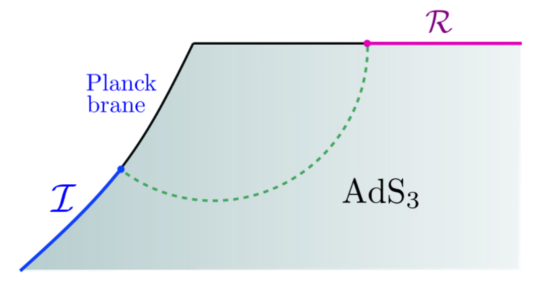
(a) Doubly holography description: AdS₃ spacetime truncated by an end-of-the-world Planck brane

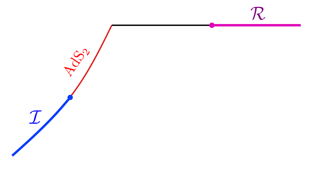
(b) Effective theory description: CFT₂ on a half line coupled to semi-classical gravity on the AdS₂ brane.

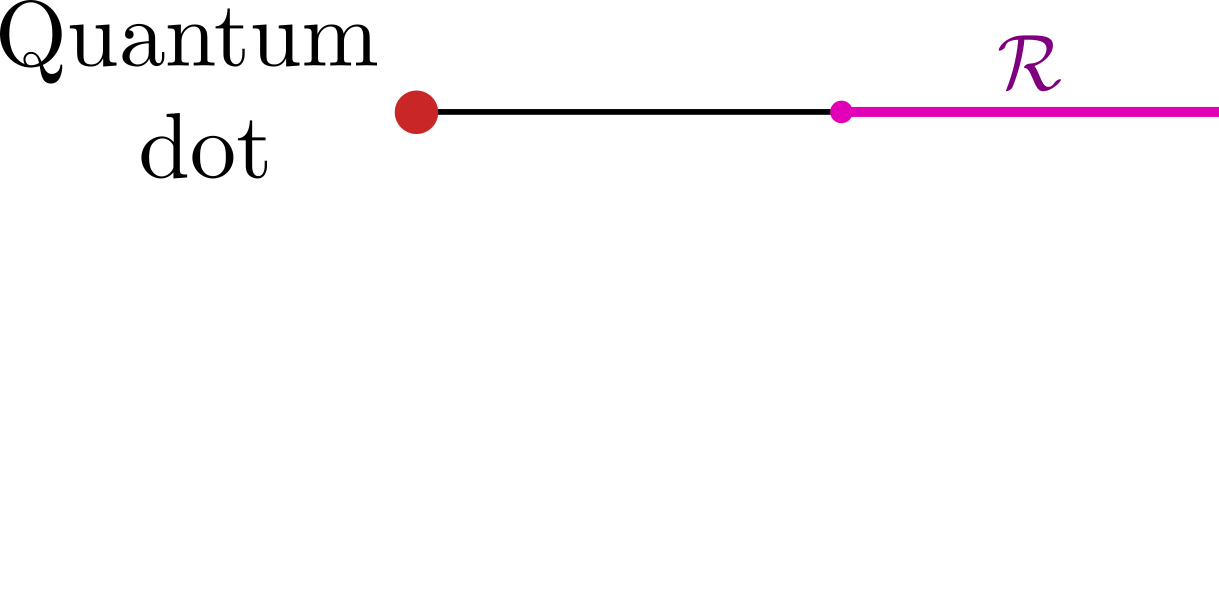
(c) Fundamental description: CFT₂ on a half line coupled to a quantum dot.

Figure 2: Three different descriptions for the same configuration.

In both of the above set-ups, gravitation plays a crucial role for the emergence of islands. It is tempting to believe that entanglement islands only exist in gravitational backgrounds. Although the island formula for $S({\rho_{\mathcal{R}}})$ reproduces the Page curve hence is consistent with unitarity, the island formula indicates that the exact density matrix $\rho_{\mathcal{R}}$ is not calculated by tracing out the degrees of freedom outside $\mathcal{R}$, rather it seems to be given by tracing out the degrees of freedom outside the region $\mathcal{R}\cup I$, i.e.

$$\rho_{\mathcal{R}}=\tilde{\rho}_{\mathcal{R}\cup I}\,.$$ (4)

This is quite surprising and counter-intuitive to our standard understanding of fundamental quantum information, if we take the semi-classical effective field theory of gravity (effective theory for short) as a usual quantum field theory in fixed curved background (curved field theory for short). The above discussion lead us to the following questions:

1. Is there anything special in the effective theory compared to the curved field theories?

2. Is gravitation essential for the emergence of entanglement islands?

3. Is it possible to understand the Island formula from a purely quantum information perspective?

These are fundamental questions and answering them will be crucial to get a deeper understanding of the entanglement islands. Furthermore, if the island formula can be understood from a purely quantum informations perspective, it may lead us to a new research field of quantum information, where we may find a way to create entanglement islands in the lab and discuss how to use them.

In this paper we propose a mechanism for the emergence of the entanglement islands in quantum systems with or without gravity. It indicates that the island phase is a fundamental property of quantum information, while those island configurations involving gravitation are just special cases. We argue that, for a generic quantum system when the Hilbert space of the total system is properly reduced following certain constraints, a island $I$ for $\mathcal{R}$ could emerge in a natural way.

• More explicitly the constraints that induce islands should be understood as projecting out certain states in the Hilbert space, such that for all the states remaining in the reduced Hilbert space, there exists a mapping from the state of the subset $\mathcal{R}$ to the state of the subset $I$, which we call a coding relation. In other words, with the Hilbert space properly reduced, given the state of $\mathcal{R}$ one can determine the state of $I$ through the coding relation.

We call systems satisfying such kind of constraints the self-encoded systems. The coding relation (or the constraints) destroys the independence between the degrees of freedom at different sites, hence essentially changes the way we calculate the reduced density matrix and related information quantities like entanglement entropy. Combining this mechanism with the discussions on entanglement islands in gravitational backgrounds, we will argue that the constraints in gravitational systems may originate from the gravitational renormalization, hence the self-encoding property is an intrinsic property of gravitational theories.

This mechanism is partially inspired by the doubly holography set-up [23], which indicates that the degrees of freedom in the island could be included as part of the entanglement wedge of $\mathcal{R}$. According to the “bulk reconstruction” program [56, 57, 14, 58, 59, 60, 61], the bulk degrees of freedom inside the entanglement wedge of a boundary region $A$ can be reconstructed from the operators inside $A$ in a quantum error correction way [59]. Although, it is still far from clear how to explicitly reconstruct the island from the radiation, it strongly indicates that the state of the island is encoded in the state of the radiation, hence gravity is self-encoded. The self-encoding property of gravity was also indicated in [40, 62, 63], which states that in gravitational theories all the information available on a Cauchy slice is also available near its boundary, which belongs to the self-encoding property described in this paper.

Another important motivation comes from a basic puzzle, which is the fact that the number of degrees of freedom in the black hole interior is divergent if we use the effective field theory description of gravity, while the number indicated by the Bekenstein-Hawking entropy is finite. If we introduce a UV cut-off to the effective description, it is even more puzzling as we note that the Bekenstein-Hawking entropy is independent from the UV cutoff. This is directly related to an long-standing problem of interpreting the black hole entropy as the entanglement entropy between the black hole interior and outside [64, 65]. Our mechanism may provide a possible answer to this puzzle in following:

• Compared with a normal curved field theory, the Hilbert space of an effective field theory is so vastly reduced, such that the UV physics in certain region are all wiped out.

In this paper we will use a Weyl transformation to simulate such a reduction in a holographic CFT₂. As we will see, the Weyl transformed holographic CFT₂ has a very similar entanglement structure as the AdS/BCFT set-up, where entanglement islands are extensively studied.

In section 2, we demonstrate our mechanism in the simplest configuration, the two-spin system under constraints such that one of the spins is determined by the other. Applying the replica trick [66, 67] to the system, we explicitly show that one of the spins can be naturally understood as the island of the other. In section 3, we consider more generic theories with more generic constraints, and show how the islands emerge. Eventually we arrive at a Island formula to calculate entanglement entropy in such systems, which include the formula (2) as a special case in gravitational theories. Based on our mechanism to interpret entanglement islands, we also provide a simple resolution to the Mathur/AMPS (Almheiri-Marolf-Polchinski-Sully) paradox [4, 5] in the three-spin self-encoded system. In section 4, we propose a non-gravitational field theory configuration to admit entanglement islands by applying certain Weyl transformation to a 2-dimensional CFT. The Weyl transformation plays the role of the constraints that reduce the Hilbert space. Furthermore, we give a proposal to create entanglement islands in many-body systems that could be synthesized in the lab. In the last section we summarize our main results, discuss the important implications or lessons we can learn from them, and their relation to other related works.

2 Reduction in two-spins system

2.1 Self-encoded quantum systems

Let us first give a general description of the self-encoded systems, where a subset $I$ can be encoded in or reconstructed from another region $\mathcal{R}$ in the system. We denote the complement of $\mathcal{R}\cup I$ by $B$. The denotations are chosen to match the black hole configurations, where $\mathcal{R}$ matches the black hole radiation in the non-gravitational reservoir, $I$ matches the island in black hole interior and $B$ matches the black hole degrees of freedom. Nevertheless, we stress that our discussion goes beyond the black hole configurations. For brevity we only consider static systems in two-dimensional spacetime with time reflection symmetry.

Firstly, let us review the computation of the reduced density matrix of $\mathcal{R}$ when the total system $I\cup B\cup R$ is in a pure state $\rho=\ket{\Psi}\bra{\Psi}$, where

$$\ket{\Psi}=\sum_{i,j,k}C_{ijk}\ket{i}_{I}\ket{j}_{B}\ket{k}_{\mathcal{R}},\qquad\sum_{i,j,k}C_{ijk}C_{ijk}^{*}=1\,.$$ (5)

Here $\{\ket{i}\},\{\ket{j}\},\{\ket{k}\}$ are the orthonormal bases of the Hilbert spaces $\mathcal{H}_{I}$, $\mathcal{H}_{B}$ and $\mathcal{H}_{R}$. In ordinary quantum systems, the degrees of freedom in different subsystems are independent, and the Hilbert space of the total system is (assumed to be) factorized,

$$\mathcal{H}=\mathcal{H}_{I}\otimes\mathcal{H}_{B}\otimes\mathcal{H}_{R}\,.$$ (6)

The reduced density matrix of the subsystem $\mathcal{R}$ is then given by tracing out the degrees of freedom of the complement $I\cup B$ while setting boundary conditions for $\mathcal{R}$ with $\bra{k_{\mathcal{R}}}$ and $\ket{k^{\prime}_{\mathcal{R}}}$,

$$\rho_{\mathcal{R}}{}_{kk^{\prime}} =\sum_{i,j}\bra{k}_{\mathcal{R}}\bra{i}_{I}\bra{j}_{B}\rho\ket{j}_{B}\ket{i}_{I}\ket{k^{\prime}}_{\mathcal{R}}=\sum_{i,j}\rho_{(ijk)(ijk^{\prime})}$$ (7)

$$=\sum_{i,j}C_{i,j,k}C_{i,j,k^{\prime}}^{*}\,.$$ (8)

As we can see, any matrix element of the reduced density matrix $\rho_{\mathcal{R}}{}_{kk^{\prime}}$ is a summation of certain class of matrix elements of the density matrix $\rho$ of the total system, which is computed within the Hilbert space $\mathcal{H}$. This implies a summation of all possibilities outside $\mathcal{R}$ for a given set of boundary conditions on $\mathcal{R}$. For a local observer who can only measure the observables inside $\mathcal{R}$, the state of $\mathcal{R}$ is exactly given by the reduced density matrix $\rho_{\mathcal{R}}$. The entanglement entropy of $\mathcal{R}$ is then calculated by

$$S_{\mathcal{R}}\equiv S(\rho_{\mathcal{R}})=-\text{Tr}\left(\rho_{\mathcal{R}}\log\rho_{\mathcal{R}}\right)\,.$$ (9)

In quantum field theories, we use the path integral representation to compute the reduced density matrix [66, 67]. More explicitly, for scenarios with time reflection symmetry, $\rho_{\mathcal{R}ij}$ for $\mathcal{R}$ can be computed by cutting $\mathcal{R}$ open and setting different boundary conditions on the upper and lower edges, see Fig.3. Then $\rho_{\mathcal{R}}^{n}$ is calculated by the replica trick via considering $n$ copies of the manifold and gluing them cyclically along the cuts present at $\mathcal{R}$. Upon taking the limit $n\to 1$ we get the entanglement entropy,

$$S(\rho_{\mathcal{R}})=S(\tilde{\rho}_{\mathcal{R}})=-\lim_{n\to 1}\partial_{n}\log\text{tr}(\rho_{\mathcal{R}}^{n}).$$ (10)

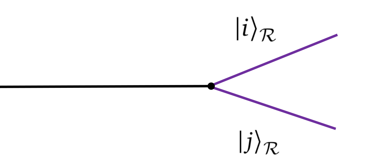
Figure 3: $\rho_{\mathcal{R}ij}$ in ordinary quantum systems represented by performing path integral with certain boundary conditions for the open edges at the region $\mathcal{R}$

The above paragraphs reviewed the standard way to compute the reduced density matrix and entanglement entropy in an ordinary quantum system. It is taken for granted that the degrees of freedom on the Cauchy slice are independent from each other and the Hilbert space factorizes following (6). Now we consider the self-encoded systems where such factorization no longer holds. We consider again a pure state of the system $I\cup B\cup\mathcal{R}$, but the system is highly constrained such that, for all the states in the reduced Hilbert space the state of the region $I$ is encoded in the state of $\mathcal{R}$ following a coding relation,

$$\ket{i}_{\mathcal{R}}\Rightarrow\ket{f(i)}_{I}\,.$$ (11)

As a mapping, this coding relation should satisfy the following two requirements,

• 1) all the states in $\mathcal{H}_{\mathcal{R}}$ should be mapped to a unique state in $\mathcal{H}_{I}$,

• 2) all the states in $\mathcal{H}_{I}$ should have at least one image in $\mathcal{H}_{\mathcal{R}}$.

The dimension of the reduced Hilbert space $\mathcal{H}_{red}$ decreases and $\mathcal{H}_{red}$ becomes a subspace of the original Hilbert space,

$$\text{dim}\mathcal{H}_{red}=\text{dim}\left(\mathcal{H}_{B}\otimes\mathcal{H}_{\mathcal{\mathcal{R}}}\right)\,,\qquad\mathcal{H}_{red}\subset\mathcal{H}_{I}\otimes\mathcal{H}_{B}\otimes\mathcal{H}_{R}\,.$$ (12)

One of the direct and crucial consequences of the self-encoding property (11) is that, the degrees of freedom in each subregion are no longer independent from each other, hence $\mathcal{H}_{red}$ is no longer factorizable following (6). In this case, the state of $I$ is determined by the state of $\mathcal{R}$ and hence $I$ does not add any independent degrees of freedom to the total system. Later we will see that, this kind of constraint will essentially change the way we construct the reduced density matrix.

2.2 The simplest case of two spins

Let us consider the simplest configuration with two spins, where we can realize our previous statements. We denote one of the spins as $I$ while denote the other as $\mathcal{R}$, and denote the spin up (down) state as $\ket{0}$ ($\ket{1}$). At the beginning, we assume the system is in the pure state

$$\rho=\ket{\Psi}\bra{\Psi}\,,\qquad\ket{\Psi}=\frac{\sqrt{2}}{2}\left(\ket{0_{I}0_{\mathcal{R}}}+\ket{1_{I}1_{\mathcal{R}}}\right)\,.$$ (13)

Firstly, let us consider the familiar scenario where the spin $I$ is independent of $\mathcal{R}$. The Hilbert space $\mathcal{H}_{I\cup\mathcal{R}}$ is four-dimensional with the following four orthonormal basis

$$\mathcal{H}_{I\cup\mathcal{R}}=\left\{\ket{0_{I}0_{\mathcal{R}}},\ket{0_{I}1_{\mathcal{R}}},\ket{1_{I}0_{\mathcal{R}}},\ket{1_{I}1_{\mathcal{R}}}\right\}\,.$$ (14)

The reduced density matrix can be calculated by, for example

$$\rho_{\mathcal{R}}{}_{00}= \bra{0_{\mathcal{R}}0_{I}}\rho\ket{0_{I}0_{\mathcal{R}}}+\bra{0_{\mathcal{R}}1_{I}}\rho\ket{1_{I}0_{\mathcal{R}}}=\frac{1}{2}\,,$$ (15)

$$\rho_{\mathcal{R}}{}_{01}= \bra{0_{\mathcal{R}}0_{I}}\rho\ket{0_{I}1_{\mathcal{R}}}+\bra{0_{\mathcal{R}}1_{I}}\rho\ket{1_{I}1_{\mathcal{R}}}=0\,,$$ (16)

and hence we find

$$\rho_{\mathcal{R}}=\begin{pmatrix}\frac{1}{2}&0\\ 0&\frac{1}{2}\end{pmatrix}\,.$$ (17)

The von Neumann entropy for $\rho_{\mathcal{R}}$ is then given by

$$S(\rho_{\mathcal{R}})=-\text{Tr}\left(\rho_{\mathcal{R}}\log\rho_{\mathcal{R}}\right)=\log 2\,,$$ (18)

which indicates that the two spins are maximally entangled with each other.

Then, we consider the new configuration with constraints on the system such that the state of the spin $I$ is somehow totally determined by $\mathcal{R}$. The mechanism is that, we impose certain constrains to project out the states with $\left\{\ket{0_{I}1_{\mathcal{R}}},\ket{1_{I}0_{\mathcal{R}}}\right\}$ components, such that the four-dimensional Hilbert space (14) reduces to the following two-dimensional one

$$Reduced:\qquad\mathcal{H}_{I\cup\mathcal{R}}=\left\{\ket{0_{I}0_{\mathcal{R}}},\ket{1_{I}1_{\mathcal{R}}}\right\}\,.$$ (19)

In this reduced Hilbert space, it is obvious that the spin of $I$ must be the same as $\mathcal{R}$, i.e.

$$Constraint:\qquad\ket{0_{\mathcal{R}}}\Rightarrow\ket{0_{I}}\,,\qquad\ket{1_{\mathcal{R}}}\Rightarrow\ket{1_{I}}\,.$$ (20)

Again, we consider the system to be in the state (13), but embed it in the reduced Hilbert space. Now it is a vector evolving in the Hilbert space (19) rather than the four-dimensional one (14). Note that, the two states $\ket{0_{I}1_{\mathcal{R}}},\ket{1_{I}0_{\mathcal{R}}}$ are no longer basis of $\mathcal{H}_{I\cup\mathcal{R}}$, and the density matrix of the total system becomes $2\times 2$ dimensional. When computing the reduced density matrix, the elements of $\rho$ appearing on the right hand side of (16) are now not well-defined.

Then how do we trace out the degrees of freedom for $I$ in the reduced Hilbert space? It turns out that, due to the constraint there is no room to perform the trace operation for $I$. More explicitly, when we set boundary conditions for $\mathcal{R}$, we are fixing the state of $\mathcal{R}$. Since the state of $I$ is totally determined by $\mathcal{R}$, we simultaneously set boundary conditions on $I$. The reduced density matrix $\rho_{\mathcal{R}}$ is then calculated by, for example

$$\rho_{\mathcal{R}}{}_{00}=\bra{0_{\mathcal{R}}0_{I}}\rho\ket{0_{I}0_{\mathcal{R}}}=\frac{1}{2}\,,$$ (21)

$$\rho_{\mathcal{R}}{}_{01}=\bra{0_{I}0_{\mathcal{R}}}\rho\ket{1_{I}1_{\mathcal{R}}}=\frac{1}{2}\,,$$ (22)

and eventually we get (see Fig.4)

$$\rho_{\mathcal{R}}=\begin{pmatrix}\frac{1}{2}&\frac{1}{2}\\ \frac{1}{2}&\frac{1}{2}\end{pmatrix}=\rho_{I\cup\mathcal{R}}\,.$$ (23)

One can further check that the von Neumann entropy for $\rho_{\mathcal{R}}$ is zero and hence $\rho_{\mathcal{R}}$ remains to be a pure state. This is expected, as we have mentioned that the additional spin $I$ does not add any independent degrees of freedom to the system. One may be confused about the way we compute $\rho_{\mathcal{R}}$ and ask why we have not traced out the degrees of freedom of $I$ in (22) as we did in (16). The reason is that, the Hilbert space (19) is reduced such that the terms in (16) are no longer matrix elements of the density matrix $\rho$. If we insist to compute following (16), then the state $\rho$ is again embedded in the four-dimensional Hilbert space and the coding relation (20) is broken, which is inconsistent with our set-up.

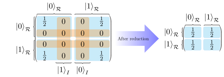
Figure 4: Illustration of the density matrice $\rho$ for the two-spin system before(LHS) and after(RHS) the reduction of the Hilbert space.

Though the two-spin system is extremely simple, we learn the following important lesson from it.

• The reduced density matrix and relevant entropy quantities not only depend on the state in which the system is settled, but also on the Hilbert space where the state is embedded in.

It is worth mentioning that, this idea can be used to clarify the ambiguity of the entanglement entropy in gauge theories (see [68, 69] and especially [70]). In gauge theories where the Hilbert space is usually redundantly labelled, the ambiguity of the entanglement entropy can naturally be understood as arising from the different choices of the Hilbert space where the state is embedded in.

3 Islands and Hilbert space reduction

3.1 Islands from more generic reductions

Now we generalize the above mechanism to more generic configurations, by imposing certain constraints such that the state of the subregion $I$ is encoded in the other region $\mathcal{R}$. Unlike the two spin system, in general the total system also includes a region $B$ where the degrees of freedom are independent. Since $I$ is totally determined by $\mathcal{R}$, it does not contribute any independent degrees of freedom. The dimension of the reduced Hilbert space $\mathcal{H}_{red}$ is then given by,

$$\text{dim}\mathcal{H}_{red}=\text{dim}\mathcal{H}_{B\cup\mathcal{R}}\,.$$ (24)

To compute the reduced density matrix for $\mathcal{R}$, again, in the path integral description we cut $\mathcal{R}$ open and set boundary conditions for the upper and lower edges at $\mathcal{R}$. Since the state of $I$ is totally determined by $\mathcal{R}$, when we set boundary conditions for $\mathcal{R}$, we simultaneously set boundary conditions at $I$. More explicitly, we should simultaneously cut $I$ open and impose certain boundary conditions on the upper and lower edges at $I$ following the coding relation (11). See Fig.5 for a illustration of the reduced density matrix $\rho_{\mathcal{R}}{}_{ij}$.

Then we calculate the entanglement entropy via the replica trick, which glues the $n$ copies of the density matrix cyclically. Since certain boundary conditions are imposed on $I$ as we set boundary conditions on $\mathcal{R}$ due to the constraints, when the boundary conditions are settled such that we cyclically glue different copies of the system at $\mathcal{R}$, the corresponding boundary conditions at $I$ following the codes (11) also imply that we simultaneously glue different copies at $I$. In other words the cyclic gluing performed on $\mathcal{R}$ induces the cyclic gluing on $I$. This results in an additional twist operator inserted at $X$, which is the boundary of $I$. In this scenario the region $I$ is nothing but the so-called “entanglement island” in the literature. As in the two-spin system, if we insist to trace out the degrees of freedom on $I$, then the calculation will involve states that are not in $\mathcal{H}_{red}$, and the encoding relation (11) will break down. In other words the notations $\tilde{\rho}_{\mathcal{R}}$ and $S(\tilde{\rho}_{\mathcal{R}})$ are ill defined.

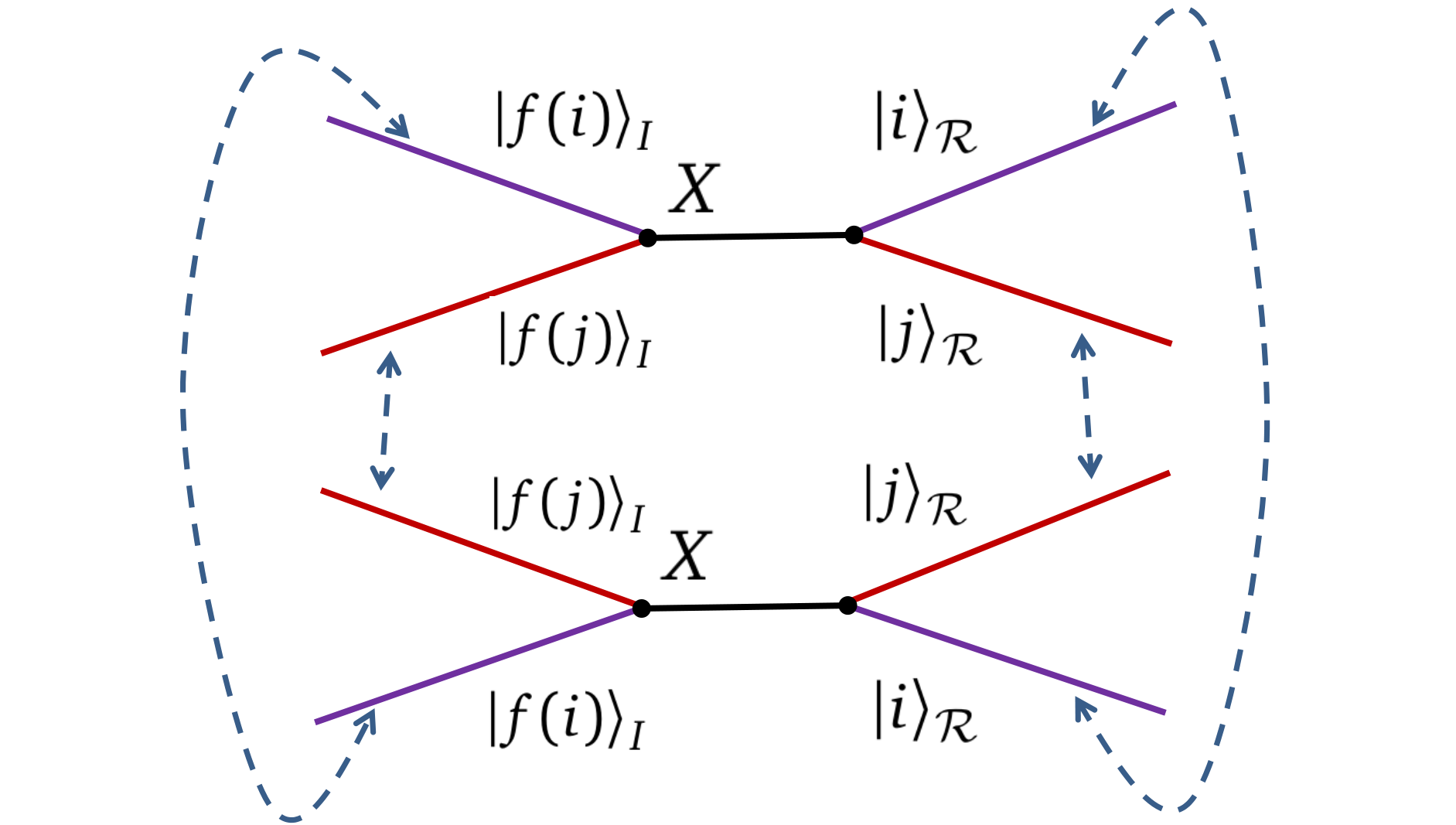
Figure 5: $\rho_{\mathcal{R}ij}$, $\rho_{\mathcal{R}ji}$ and $\text{Tr}\rho_{\mathcal{R}}^{2}$ in self encoding quantum systems with $I$ encoded in $\mathcal{R}$.

Let us denote

$$\tilde{S}_{\mathcal{R}}\equiv S(\tilde{\rho}_{\mathcal{R}})\,,$$ (25)

as the von Neumann entropy calculated by cyclically gluing only the region $\mathcal{R}$ in replica trick. In ordinary systems where the Hilbert space is not reduced, we have the trivial relation $S_{\mathcal{R}}=\tilde{S}_{\mathcal{R}}$ Nevertheless, in the self-encoded configurations we currently consider, this relation no longer holds. Based on the above discussions, we arrive at the following crucial relation for self-encoded systems

$$S_{\mathcal{R}}=\tilde{S}_{\mathcal{R}\cup I}\,.$$ (26)

This looks quite similar to the island formula (2) proposed in gravitational systems with one important difference that, here we do not have the area term.

Note that, in the above discussion the system is a non-graviational quantum system. If $I$ is settled on a gravitational background while $\mathcal{R}$ is settled in a non-gravitational bath, then according to [11, 26, 27] we will receive additional gravitational contribution, which is proportional to the area of the fixed points of the replica symmetry, i.e. the boundary $X$ of $I$ where the additional twist operator is inserted. The non-gravitational part of $\tilde{S}_{\mathcal{R}\cup I}$ is also called the bulk entanglement entropy $S_{bulk}({\tilde{\rho}_{\mathcal{R}\cup I}})$ which is calculated in a fixed curved background. Eventually we arrive at the following formula

$$Island~{}formula~{}II:\quad S_{\mathcal{R}}=\tilde{S}_{\mathcal{R}\cup I}=S_{bulk}({\tilde{\rho}_{\mathcal{R}\cup I}})+\frac{Area(X)}{4G}\,,\quad\ket{i}_{\mathcal{R}}\Rightarrow\ket{f(i)}_{I}\,,$$ (27)

which exactly matches to the formula within the parenthesis in the island formula $I$ in (2).

3.2 Self-encoding property from gravitational renormalization?

The self-encoding property gives a natural interpretation for the emergence of entanglement islands in quantum information. More importantly, it seems to be the only plausible interpretation, which indicates that when entanglement island emerges in a quantum system, the system should be self-encoded. Then it is very tempting to claim that the Island formula I is a special application of the Island formula II in gravitational theories. A crucial conclusion we can make from this claim is that:

• The self-encoding property is an intrinsic property of gravitational theories. For the specific case of a black hole after the Page time, the state of the entanglement island in the black interior is encoded in the state of the Hawking radiation.

Nevertheless, there are important differences between the two island formulas (2) and (27) which we need to clarify. Most importantly, the existence of gravitation is essential for the derivation of island formula (2), and it is not obvious that whether there are constraints imposed on the system. For systems where Island formula I applies, gravitation allows us to consider all the geometric configurations hence the replica wormholes arise as new saddle points in the path integral computation of the partition function on the replicated manifold. In such a way the entanglement island emerges from these new geometric saddles. According to our discussion in the last subsection, to be consistent with quantum information the self-encoding property is indicated by such replica wormhole geometries. While in (27), the island $I$ appears naturally from the self-encoding property, which is a result of imposing certain constraints, and gravitation is not necessary.

If Island formula I is a special case of Island formula II, then the existence of the new dominant replica wormhole saddle should also be a result of certain constraints which reduce the Hilbert space of the curved field theory properly. Where are the constraints? For a curved field theory the dimension of the Hilbert space (or number of degrees of freedom) is infinite, and all the degrees of freedom on a given Cauchy slice should be independent from each other. One can renormalize the theory by introducing a UV-cutoff $\Lambda$ everywhere, hence the number of degrees of freedom becomes a finite number depending on $\Lambda$. The Hilbert space is reduced under the renormalization, but no coding relation emerges as the degrees of freedom at different sites are still independent. If our claim is true, then an effective theory must be something different from a curved field theory with a UV cutoff. In the following we provide some clues in support of this conjecture.

In a gravitational theory with a black hole, according to the Bekenstein-Hawking entropy formula the number of independent degrees of freedom inside the black hole is captured by the area of the black hole horizon divided by $4G$, which is a finite number that does not depend on the choice of the UV-cutoff $\Lambda$. However, if we consider the effective theory of gravity to be some curved field theory, the number of independent degrees of freedom should be proportional to the volume of the black hole interior and depends on the UV cutoff $\Lambda$. It seems that the effective theory can be taken as a curved field theory with the Hilbert space vastly reduced, but with no manifest extrinsic constraints.

Then where do the constraints come from? Is the constraints intrinsic in gravitational theories? We may find some clues from the calculation of the entanglement entropy of black holes. For example, one can consider a curved field theory in a black hole background, and consider a Cauchy slice where the black hole horizon (or bifurcation surface) $\Sigma$ splits it into the black hole interior and black hole exterior. Let us consider a four-dimensional gravity theory minimally coupled to a massless scalar. One can calculate the entanglement entropy between the black hole interior and exterior via the replica method, the tree level entropy and one-loop level entropy are given by [73, 74]

$$S_{tree}=\frac{1}{4G_{B}}A(\Sigma)\,,\qquad S_{one-loop}=\frac{1}{48\pi\epsilon^{2}}A(\Sigma)\,.$$ (28)

The parameter $\epsilon$ represent the UV cutoff scale of the curved field theory, and $G_{B}$ is the bare Newton’s constant. Following the standard procedure of gravitational renormalization (see for instance [76]), one can renormalize the UV divergences of the gravitational action by absorbing them into a redefinition of the couplings. For our case, we have

$$\frac{1}{G_{ren}}=\frac{1}{G_{B}}+\frac{1}{12\pi\epsilon^{2}}\,,$$ (29)

where $G_{ren}$ is the renormalized Newton constant that we can measure. Remarkably, such a redefinition of the couplings automatically renormalizes the UV divergent part in the entanglement entropy,

$$S_{ren}=\frac{1}{4G_{B}}A(\Sigma)+\frac{1}{48\pi\epsilon^{2}}A(\Sigma)=\frac{1}{4G_{ren}}A(\Sigma)\,.$$ (30)

All in all, in this case after we perform the gravitational renormalization, the UV dependence of the entanglement entropy vanishes and we get a finite entanglement entropy for a field theory.

• It seems that the gravitational renormalization turns off the physics at UV by introducing finite cutoff to the curved field theory, hence vastly reduces the Hilbert space. The curved field theory together with the finite cutoff configuration are what make the effective theory.

If this is the case, then the constraints in gravitational theories that result in the self-encoding property could be intrinsic and originate from the gravitational normalization. In this paper we will not discuss how explicitly the gravitational renormalization introduces the finite cutoff, but we will give an example of finite cutoff configuration in an effective theory and discuss how entanglement island emerge from the finite cutoff in the next section.

Before we go ahead, we need to clarify another important difference between the two island formulas. In (2) the island region $I$ is determined by extremizing the entropy among all the choices of $I$, and the region $I$ can be recognized as a entanglement island only when the island formula (2) gives smaller entanglement entropy than $\tilde{S}_{R}$. This difference can be explained by a special coding-relation in the gravitational systems, which is much more complicated than the coding-relation we have discussed previously. In other words, in principle it is possible to find a coding-relation such that the island $I$ resulting from this coding-relation following the Island formula II coincide with the islands resulting from the extremal condition in the Island formula I. We leave this for future investigations.

3.3 Requirements for the Hilbert space reductions

The self-encoding constraints (11) is only one particular way to reduce the Hilbert space of the system. There are certainly other ways to reduce the Hilbert space, among which one will be introduced in later sections where the eliminated degrees of freedom are not localized in a definite spatial region. Nevertheless, not all reductions will essentially change the reduced density matrix and some of them are not even well defined. Here we present the following four requirements for the type of Hilbert space reductions which are interesting to us:

• first of all, the state $\ket{\Psi}$ under consideration should remain in the reduced Hilbert space;

• secondly, when we impose boundary conditions for $\mathcal{R}$, we should have a square matrix block in $\rho$ from which the corresponding element of the reduced density matrix can be computed by tracing out the matrix block;

• thirdly, since we would like to study the reduced density matrix of the region $\mathcal{R}$ under reduction without reducing the degrees of freedom of $\mathcal{R}$, we require that the reduction is required to only reduce the degrees of freedom of the complement $\bar{\mathcal{R}}$, hence the dimension of $\rho_{\mathcal{R}}$ is still $\text{dim}\mathcal{H}_{\mathcal{R}}$;

• at last, the reduction is expected to change the von Newmann entropy of the reduced density matrix $\rho_{\mathcal{R}}$.

The second requirement implies that, after the reduction of the Hilbert space, the degrees of freedom for the complement $\bar{\mathcal{R}}$ should be preserved, no matter in which state the subsystem $\mathcal{R}$ is settled. For example, we can reduce the Hilbert space of the two-spins system to be

$$\mathcal{H}_{I\cup\mathcal{R}}=\{\ket{0_{I}0_{\mathcal{R}}},\ket{1_{I}0_{\mathcal{R}}},\ket{1_{I}1_{\mathcal{R}}}\}\,,$$ (31)

in which $I$ is fixed to be the same as $\mathcal{R}$ when $\mathcal{R}$ is in the state $\ket{1_{\mathcal{R}}}$. On the other hand when $\mathcal{R}$ is in the state $\ket{0_{\mathcal{R}}}$, there is no constraint on the spin $I$. In other words the degrees of freedom of $I$ differ depending on the state of $\mathcal{R}$, hence our second requirement is not satisfied. This could be problematic, since when setting boundary conditions for $\mathcal{R}$ and computing the elements of $\rho_{\mathcal{R}}$, we will find that the matrix block is no longer a square matrix, which means that the degrees of freedom of $I$ cannot be described in the usual sense of a density matrix anymore. One should further study and define the physical meaning of density matrix blocks that are not square. Nevertheless, this is beyond the scope of this paper and we will naively consider such reductions to be un-physical. One necessary condition for the second requirement is that, the dimension of the reduced Hilbert space should be an integer times $\dim\mathcal{H}_{\mathcal{R}}$. As an explicit example, we consider a vector $\ket{a}$ in the Hilbert space of the two-spins system before reduction

$$\ket{a}=\frac{1}{\sqrt{3}}\left(\ket{0_{I}0_{\mathcal{R}}}+\ket{1_{I}0_{\mathcal{R}}}+\ket{1_{I}1_{\mathcal{R}}}\right)\,,$$ (32)

and the corresponding density matrix in the unreduced Hilbert space can be worked out as depicted on the left panel of Fig.6. After reducing the Hilbert space to $\mathcal{H}_{I\cup\mathcal{R}}$ in (31) in which the degrees of freedom of $I$ depend on the state in $\mathcal{R}$, the density matrix can be shown to be given in the form of the right panel of Fig.6. The matrix elements in the orange area all vanish since the state $\ket{a}$ does not contain any $\ket{0_{I}1_{\mathcal{R}}}$ component, which is the constraint from our first requirement. The matrix blocks enclosed by the purple areas are not square which is different from density matrices before the reduction of Hilbert space. Thus, the reduced density matrix after the reduction of the Hilbert space is not well-defined in the usual way and this is exactly the point of our second requirement.

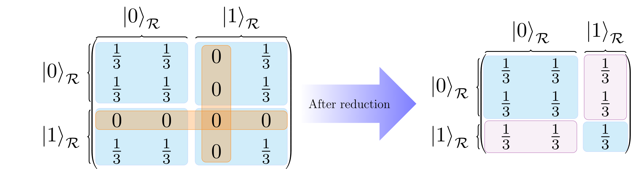
Figure 6: Illustration of the density matrices of $\ket{a}$ before(LHS) and after(RHS) the reduction of the Hilbert space.

The third requirement implies that, in the reduced Hilbert space of the total system the state of $\mathcal{R}$ can be any state in $\mathcal{H}_{R}$. Under such a requirement we are tempted to choose the reductions which still contain a factor of $\mathcal{H}_{\mathcal{R}}$ in the reduced Hilbert space, i.e.

$$\mathcal{H}=\mathcal{H}_{\bar{\mathcal{R}}}\otimes\mathcal{H}_{\mathcal{R}}\quad{Reduction}:\quad\mathcal{H}=\mathcal{H}_{B}\otimes\mathcal{H}_{\mathcal{R}}\,,\qquad\mathcal{H}_{B}\subset\mathcal{H}_{\bar{\mathcal{R}}}\,.$$ (33)

These reductions automatically satisfy the second requirement. Then we consider the a state $\ket{\Psi}\in\mathcal{H}_{B}\otimes\mathcal{H}_{\mathcal{R}}$, which is now embedded in the original Hilbert space $\mathcal{H}_{\bar{\mathcal{R}}}\otimes\mathcal{H}_{\mathcal{R}}$. When we set boundary conditions for $\mathcal{R}$, the block matrix in $\rho$ becomes a $\text{dim}\mathcal{H}_{\bar{\mathcal{R}}}$ dimensional square matrix, which contains the $\dim\mathcal{H}_{B}$ dimensional block matrix of $\rho$ in the reduced case as a sub-block. While all the other elements in the block outside the sub-block are zero. The reason is that in the state $\ket{\Psi}$ we consider, the sub-system $\bar{\mathcal{R}}$ is confined entirely in the subspace $\mathcal{H}_{B}$. The von Neumann entropy of $\rho_{\mathcal{R}}$ does not change after reduction, hence the last requirement is not satisfied. One can also check that the reduced Hilbert space (19) for the two-spins system which leads to a different entanglement entropy does not factorize following (33).

It will be interesting to explore other ways of reduction that satisfy our four requirements beyond the self-encoded systems.

3.4 Islands beyond spatial regions

Now we introduce a class of reductions where the reduced degrees of freedom in $\bar{\mathcal{R}}$ are not localized in a spatial subregion $I$. These reductions also satisfy the above four requirements. Let us use two sets of parameters $\{a_{i}\}$ and $\{b_{j}\}$ to denote the states in the Hilbert space $\mathcal{H}_{\bar{\mathcal{R}}}$ as follows

$$\ket{a_{1},a_{2}\cdots a_{n},b_{1},b_{2}\cdots b_{m}}_{\bar{\mathcal{R}}}\in\ket{\mathcal{V}_{a}\otimes\mathcal{V}_{b}}=\mathcal{H}_{\bar{\mathcal{R}}}\,.$$ (34)

and a generic state for the entire system can be expressed by

$$\ket{\Psi}=\sum_{a_{1},\cdots a_{n},b_{1},\cdots b_{m},i}C_{a_{1},\cdots a_{n},b_{1},\cdots b_{m},i}\ket{a_{1},\cdots a_{n},b_{1},\cdots b_{m}}_{\bar{\mathcal{R}}}\ket{i}_{\mathcal{R}}\,.$$ (35)

Here, for example, $\mathcal{V}_{a}$ represents a vector space in which a generic vector can be specified by the set of parameters $\{a_{i}\}$. It is not the Hilbert space of $a$, since $a$ is not a subregion of $\bar{\mathcal{R}}$.

Now we reduce the Hilbert space following certain constraints. We assume that the state of $\mathcal{R}$ determines the parameters $\{a_{i}\}$ in the following way

$$\ket{i}_{\mathcal{R}}\quad\Rightarrow\quad\ket{\vec{f}(i),b_{1},b_{2}\cdots b_{m}}_{\bar{\mathcal{R}}}\,,$$ (36)

where $\vec{f}(i)$ is a vector in the space $\mathcal{V}_{a}$. This means that for any state $\ket{\Psi}$ in the reduced Hilbert space, if the state of the subregion $\mathcal{R}$ is $\ket{i}_{\mathcal{R}}$, then the corresponding state of $\bar{\mathcal{R}}$ in the state $\ket{\Psi}$ is partially determined with the parameters in the subspace $\mathcal{V}_{a}$ fixed to be $\vec{f}(i)$. Hence the dimension of the Hilbert space reduces to be $\text{dim}(\mathcal{V}_{b})\times\text{dim}(\mathcal{H}_{\mathcal{R}})$. In the reduced Hilbert space, a generic state $\ket{\Psi}$ can be expressed by

$$\ket{\Psi}=\sum_{b_{1},b_{2}\cdots b_{m},i}C_{b_{1},b_{2}\cdots b_{m},i}\ket{\vec{f}(i),b_{1},b_{2}\cdots b_{m}}_{\bar{\mathcal{R}}}\ket{i}_{\mathcal{R}}\,.$$ (37)

Note that, in the reduced Hilbert space the independent degrees of freedom are confined in the subspace $\mathcal{V}_{b}$, which are usually parameters characterizing the state of $\bar{\mathcal{R}}$, rather than a subset $I$ inside $\bar{\mathcal{R}}$. Then the reduced density matrix is calculated by

$$\rho_{\mathcal{R}ij}=\sum_{b_{1},b_{2}\cdots b_{m}}C_{b_{1}\cdots b_{m},i}C^{*}_{b_{1}\cdots b_{m},j}\ket{\vec{f}(i),b_{1},\cdots b_{m}}_{\bar{\mathcal{R}}}\bra{\vec{f}(j),b_{1},\cdots b_{m}}_{\bar{\mathcal{R}}}\,,$$ (38)

where we have only traced the independent degrees of freedom in $\mathcal{V}_{b}$.

In this type of reductions (36) the reduced degrees of freedom in $\mathcal{V}_{a}$ are not required to be mapped to the degrees of freedom localized in any spacial region $I$ inside $\bar{\mathcal{R}}$, hence there could be no spatial region $I$ that plays the role of an island. Rather, the island is a sub-space in the parameter space which characterize the Hilbert space.

3.5 The resolution of the Mathur/AMPS paradox in a toy model

The authors of [4, 5] pointed out that, the Mathur/AMPS puzzle in quantum information for the process of black hole evaporation already appears after the Page time, if black hole evaporation is assumed to be unitary. The Mathur/AMPS paradox points out that an impossible quantum state emerges after the Page time. Let us assume unitarity and consider a black hole which is collapsed from a quantum system in a pure state. After the Page time the late radiation should be maximally entangled with the early radiation, hence purifies the early radiation. On the other hand, this quanta of late radiation should also be maximally entangled to its partner quanta inside the black hole if the horizon is smooth. However, according to monogamy of entanglement, a given quanta cannot be maximally entangled to two separate systems, otherwise the strong subadditivity of the entropy will be violated. A resolution was provided in [5] which discards the entanglement between the late radiation and its partner in the interior by forming a "firewall" at the horizon.

Now we try to understand this paradox based on our previous discussion. Again let us denote the late radiation quanta and its partner in the interior as $B$ and $I$, while denote the early radiation quanta that was purified by $B$ as $\mathcal{R}$. Note that, the statement that $B$ cannot be maximally entangled to $\mathcal{R}$ and $I$ simultaneously, is built on the pre-condition that, all the three qubits are independent degrees of freedom such that the Hilbert space $\mathcal{H}$ factorizes in the following way

$$\mathcal{H}=\mathcal{H}_{I}\otimes\mathcal{H}_{B}\otimes\mathcal{H}_{\mathcal{R}}\,.$$ (39)

Although, this pre-condition is usually taken for granted, it is invalid when we set constraints on the whole system. Furthermore, as we have shown previously, under a proper reduction of the Hilbert space the computation of the reduced density matrix, as well as the related entropy quantities, will change essentially. For example, let us consider the following state for a three-spin system,

$$\ket{\Psi}=\frac{\sqrt{2}}{2}\left(\ket{1_{I}0_{B}1_{\mathcal{R}}}+\ket{0_{I}1_{B}0_{\mathcal{R}}}\right)\,.$$ (40)

Then we consider the Hilbert space is reduced by imposing the requirement that the spin of $I$ should be the same as $\mathcal{R}$, hence one of them is not an independent degrees of freedom. The observer outside the black hole will take the qubit $\mathcal{R}$ as the independent one, and conclude that the two qubits $\mathcal{R}$ and $B$ are maximally entangled. While an infalling observer would take $I$ as the independent one and claim that the two qubits $B$ and $I$ are maximally entangled. However, for the outsider observer who take $I$ to be not independent, the entanglement between $I$ and $B$ is not well defined, or just vanished. Hence $B$ is not maximally entanglement to $\mathcal{R}$ and $I$ simultaneously, and the monogamy of entanglement is not violated.

Provided that $I$ belongs to the entanglement island thus is not independent, the Mathur/AMPS puzzle is resolved in the reduced Hilbert space. If we embed this system into the black hole evaporation process, then we face a quantum information problem in the following. We have a constraint that the quanta at the horizon is maximally entanglement with the early radiation $\mathcal{R}$. Then after horizon quanta decays into $I$ and $B$, how does this constraint reduce the Hilbert space such that the interior quanta $I$ becomes non-independent while the outside quanta $B$ inherits its entanglement structure with $\mathcal{R}$? Or do we need more constraints? Solving this problem may help us understand how exactly the information are transferred from the black hole to the radiation.

4 A simulation of Hilbert space reduction via Weyl transformation

Previously we proposed that Island formula I is a special case of Island formula II, and the constraints leading to the coding relation in the effective theory is a result of the finite cutoff configuration induced by the gravitational renormalization. Inspired by the doubly holography [23] set-up or AdS/BCFT correspondence [78], in this section we introduce the finite cutoff configuration via a Weyl transformation for a holographic CFT₂. We will discuss the entanglement structure and the emergence of entanglement islands in this configuration.

4.1 Finite cutoff from Weyl transformation in CFT₂

Let us start from the vacuum state of a holographic CFT₂ on a Euclidean flat space

$$ds^{2}=\frac{1}{\delta^{2}}\left(d\tau^{2}+dx^{2}\right)\,.$$ (42)

Here $\delta$ is an infinitesimal constant representing the UV cutoff of the boundary CFT. The theory is invariant under the Weyl transformation of the metric

$$ds^{2}=e^{2\varphi(x)}\left(\frac{d\tau^{2}+dx^{2}}{\delta^{2}}\right)\,.$$ (43)

This effectively changes the cutoff scale in the following way

$$\delta\Rightarrow e^{-\varphi(x)}\delta\,.$$ (44)

The entanglement entropy of a generic interval $\mathcal{R}=[a,b]$ in the CFT after the Weyl transformation picks up additional contributions from the scalar field ${\varphi}(x)$ as follows [79, 80, 81]

$$S_{\mathcal{R}}=\frac{c}{3}\log\left(\frac{b-a}{\delta}\right)+\frac{c}{6}{\varphi}(a)+\frac{c}{6}{\varphi}(b)\,.$$ (45)

This formula can be achieved by performing the Weyl transformation on the two-point function of the twist operators.

Before we go ahead, we give a physical interpretation for the Weyl transformation, as well as the entropy formula (45). Before the Weyl transformation the UV cutoff of the CFT is a uniform infinitesimal constant $\delta$. The Weyl transformation is indeed a scale transformation that changes the cutoff scale of the system at each point. Such a non-uniform cutoff would definitely affect the multi-scale entanglement structure for the CFT. After the Weyl transformation, the formula (45) tells us that the entanglement entropy is just the original one subtracting two constants which are totally determined by the scalar field at the two endpoints. More importantly the subjected constant is independent from the position of the other endpoint, as long as the two endpoints are not close enough to give a negative entanglement entropy following (45). Hence we conclude that, the Weyl transformation at any point effectively excludes all the small distance entanglement across this point below the cutoff scale, which is a constant, while keeping the long distance entanglement unaffected.

For our purpose to study entanglement islands, we perform a specific Weyl transformation on a holographic CFT₂ that corresponds to Poincaré AdS₃, such that the metric becomes AdS₂ in the $x<0$ region and remains flat in the $x>0$ region. Such a Weyl transformation can be easily found to be

$$\varphi(x)=\begin{cases}0\,&,\text{if}\quad x>0\,,\\ \\ -\log\left(\frac{2|x|}{\delta}\right)+\kappa\,.\,&,\text{if}\quad x<0\,,\end{cases}$$ (46)

where $\kappa$ is an undetermined constant. The corresponding metric at $x<0$ after the Weyl transformation becomes

$$ds^{2}=\frac{e^{2\kappa}}{4}\left(\frac{d\tau^{2}+dx^{2}}{x^{2}}\right)\,,\qquad x<0\,.$$ (47)

As expected, the above metric is AdS₂ up to an overall coefficient (the length scale is given by $e^{\kappa}/2$). Note that, in order to get a AdS₂ metric independent of $\delta$, we need to choose a scalar field depending on $\delta$ which goes to infinity when $\delta\to 0$. The specific choice (46) for the scalar field is made to simulate the entanglement structure for the AdS/BCFT correspondence, where the effective theory description can be taken as an AdS₂ gravity coupled to a CFT₂ bath. Also the cutoff scale in the $x<0$ region is no longer infinitesimal, rather the cutoff scale is bounded from below and depends on the position $x$.

4.2 Weyl transformed CFT vs AdS/BCFT

The AdS/BCFT [78] correspondence is a widely used setup where entanglement islands emerge. The basic statement is that, the holographic CFT₂ with a boundary correspond to the AdS₃ bulk with a end of world (EoW) brane which extends in the bulk and anchors on the boundary of the CFT. In the AdS₃ bulk, the EoW brane satisfies Neumann boundary condition and its position is determined by its tension. In this setup, it is more convenient to use another set of coordinates $(t,\rho,y)$ to describe the AdS₃ bulk geometry,

$$x=y\tanh\rho~{}~{},~{}~{}z=-y\text{sech}\,\rho\,.$$ (48)

The bulk metric in these coordinates is given by the standard Poincaré slicing, as follows

$$ds^{2} =d\rho^{2}+\cosh^{2}\rho\frac{-dt^{2}+dy^{2}}{y^{2}}=\frac{-dt^{2}+dx^{2}+dz^{2}}{z^{2}}\,,$$

where the AdS₃ radius is set to be unity. In the Poincaré slicing described by the $(t,\rho,y)$ coordinate chart the EoW brane is situated at a constant $\rho=\rho_{0}$ slice [82], where $\rho_{0}$ is determined by the tension $T$ of the EoW brane,

$$\rho_{0}=\text{arctanh}T\,.$$ (49)

It is easy to see that the metric on the EoW brane is exactly AdS₂ up to an overall constant. The key property in the AdS/BCFT setup is that, the RT surface $\mathcal{E}_{\mathcal{R}}$ of a boundary region $\mathcal{R}$ is also allowed to be anchored on the EoW brane $\mathbb{Q}$ [78, 82] (see Fig.7). This was confirmed in [83] via a direct computation of the correlation functions of twist operators in BCFTs with large central charge. Hence, new configurations for the RT surfaces that anchors on $\mathbb{Q}$ arise in AdS/BCFT. The island formula in doubly holography setups is reproduced by considering these new configurations of the RT surfaces when applying the RT formula to calculate the holographic entanglement entropy.

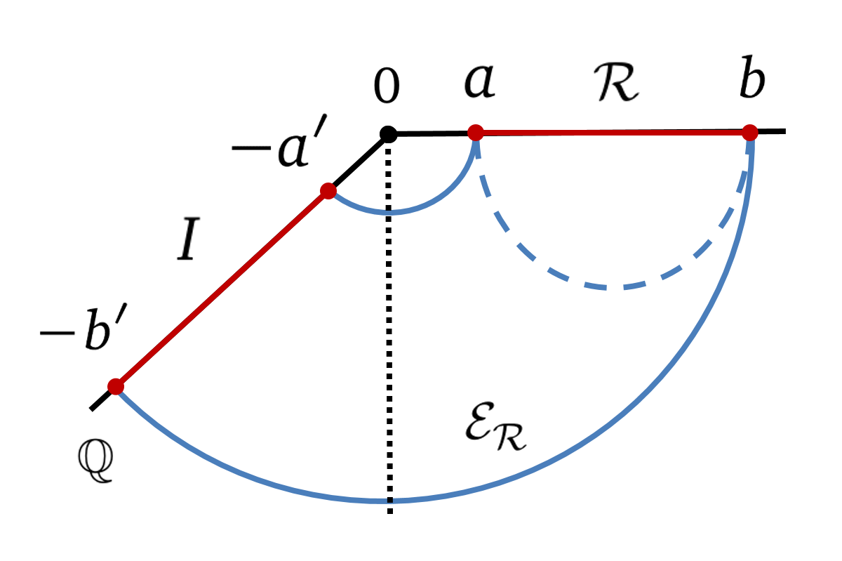
Figure 7: Holographic entanglement entropy in the AdS/BCFT setup: (left) For an interval $\mathcal{R}=[a,\infty]$ in the BCFT, the RT surface has the disconnected topology and lands on the EoW brane at $a^{\prime}=a$. (right) For $\mathcal{R}=[a,b]$, the connected(disconnected) RT surfaces are shown by the blue dashed(solid) curves. The position where $\mathcal{E}_{\mathcal{R}}$ anchors on $\mathbb{Q}$ is determined by extremizing the length of $\mathcal{E}_{\mathcal{R}}$, which gives $a^{\prime}=a$ and $b^{\prime}=b$. The dashed vertical line denote the $\rho=0$ slice.

For example, the entanglement entropy of the region $\mathcal{R}:=[a,\infty)$ may be computed through the length of the RT curve $\mathcal{E}_{\mathcal{R}}$ homologous to $\mathcal{R}$ and anchored on the EoW brane. After determining the location on the brane by extremizing the length of $\mathcal{E}_{\mathcal{R}}$ (see the left panel in Fig.7), the holographic entanglement entropy is given by

$$S_{\mathcal{R}}=\frac{Area(\mathcal{E}_{\mathcal{R}})}{4G}=\frac{c}{6}\log\left(\frac{2a}{\delta}\right)+\frac{c}{6}\rho_{0}\,.$$ (50)

Note that the area term $\frac{Area(\mathcal{E}_{\mathcal{R}})}{4G}$ captures the bulk entanglement entropy term in the Island formula I, while the area term $\frac{AreaX}{4G}$ is ignored by taking the gravity theory settled on the EoW brane to be the induced gravity by partial reduction on the $\rho_{0}>\rho>0$ region. This choice is necessary to compare with the configuration of the holographic Weyl transformed CFT₂ later. For the choice $\mathcal{R}:=[a,b]$ there are two possible saddles for the RT surface, one is a connected geodesic that anchored on the two endpoints of $\mathcal{R}$, while the other consists of two disconnected geodesics which also anchor on the EoW brane $\mathbb{Q}$ (see the right panel in Fig.7). The holographic entanglement entropy is simply given by

$$S_{\mathcal{R}}=\begin{cases}\frac{c}{3}\log\left(\frac{b-a}{\delta}\right)\,&,\,\text{if}\quad a>b\left(1-2\sqrt{e^{2\rho_{0}}+e^{4\rho_{0}}}+2e^{2\rho_{0}}\right)\,,\\ \\ \frac{c}{6}\log\left(\frac{2a}{\delta}\right)+\frac{c}{6}\log\left(\frac{2b}{\delta}\right)+\frac{c}{3}\rho_{0}\,.\,&,\,\text{if}\quad 0<a<b\left(1-2\sqrt{e^{2\rho_{0}}+e^{4\rho_{0}}}+2e^{2\rho_{0}}\right)\,.\end{cases}$$ (51)

In both left and right panels in Fig. 7, the portion of the brane $\mathbb{Q}$ (marked red) lying in the entanglement wedge of $\mathcal{R}$ are be interpreted as the island region from a doubly holographic point of view.

Now we return to the Weyl transformed CFT and compare with the version of island formula in the AdS/BCFT or doubly holographic setup. The physical interpretation for Weyl transformation is more intuitive if the CFT is holographic, hence the entanglement structure has a geometric interpretation. Before we perform the Weyl transformation, the vacuum state of the CFT is dual to Poincaré AdS₃ (41). And according to the RT formula the entanglement entropy for any interval is given by the length of the minimal bulk geodesic homologous to this interval. The integral computing the length of the RT surface represents the collection of the entanglement at all the scales [84]. In this context, the Weyl transformation adjusts the cutoff scale by adjusting the position of the cutoff point on the RT curve, where we stop integrating the length of the RT curve. According to the formula (45), for any RT surface anchored at the site $x_{0}$ on the boundary, we need to push the cutoff point on the RT surface from $z=\delta$ to certain position in the bulk, such that the length of the RT surface is reduced by certain constant $|{\varphi}(x_{0})|$. In other words the cutoff points for all the RT curves anchored at $(\delta,x_{0})$ form a sphere in the bulk. Interestingly, for static configurations, the cutoff sphere in the AdS₃ background is a circle in flat background,

$$\left(x-x_{0}\right){}^{2}+\left(z-|x_{0}|e^{-\kappa}\right)^{2}=|x_{0}|^{2}e^{-2\kappa}\,,$$ (52)

with the center being $(|x_{0}|e^{-\kappa},x_{0})$ and the radius $r=|x_{0}|e^{-\kappa}$. One may consult Appendix A for the derivation. The formula (45) then can be understand as follows: when we integrate the length of the RT surface, we only integrate up to the cutoff sphere (see Fig.8).

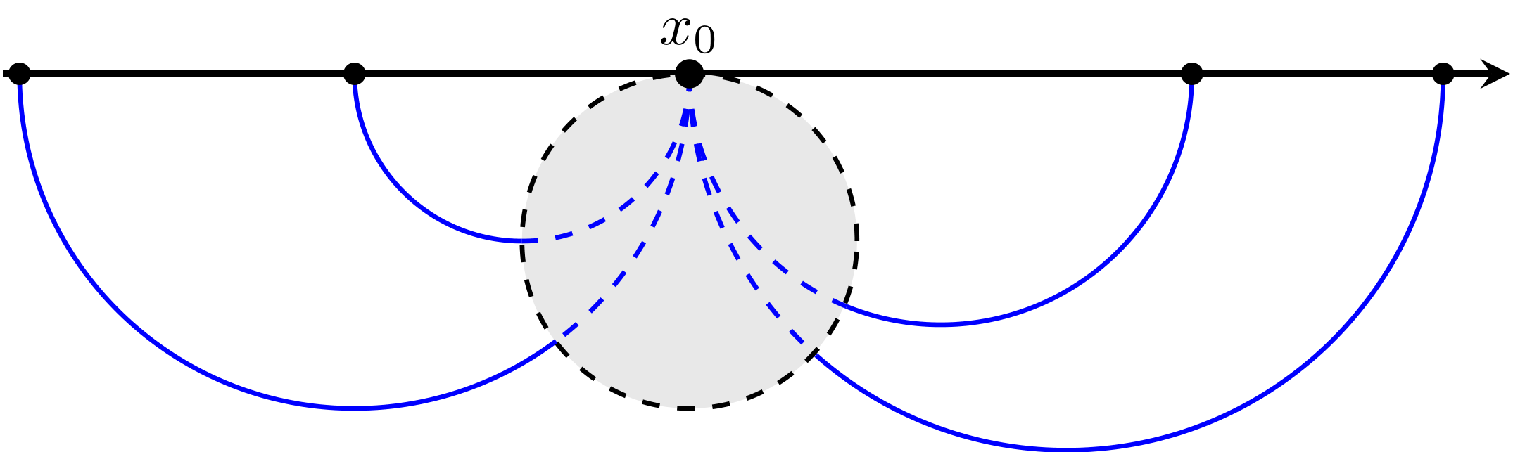
Figure 8: Cutoff sphere at $x=x_{0}$ in the bulk dual geometry for a Weyl transformed CFT. For a minimal surface anchored at $x_{0}$, the portion inside the cutoff sphere is excluded.

The Weyl transformation (46) then adjusts the cutoff scale in the region $x<0$. In some sense, this pushes the cutoff slice from $z=\delta$ into the bulk. Here the cutoff slice can be identified as the common tangent line of all the cutoff spheres. Interestingly, we find that this common tangent line is just given by $\rho=\kappa$, see appendix A for details. This reminds us of the EoW brane in the AdS/BCFT setup, which is also settled at a constant $\rho$ slice. The common tangent line indeed plays a quite similar role as the EoW brane $\mathbb{Q}$, see Fig. 9. Most importantly, the RT surfaces are also allowed to anchor on the tangent line, in the sense that the RT surfaces are cut off at this line. Also the degrees of freedom behind the tangent line all belongs to certain cutoff spheres, hence the tangent line seems like a end of world line. More interestingly, if we apply Island formula I to this Weyl transformed CFT₂, we will find configurations with islands which give smaller entanglement entropy than the non-island configurations. This is a result of the finite cutoff introduced by the Weyl transformation. In the following, we will see that the calculation exactly coincides with the entanglement entropies in the AdS/BCFT setup.

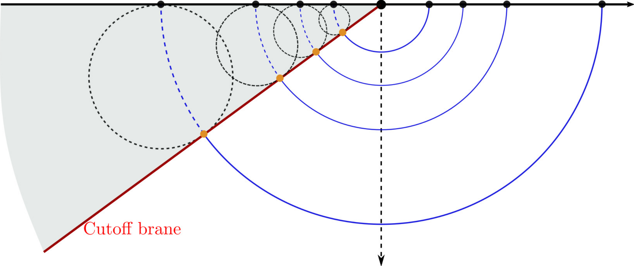
Figure 9: The common tangent surface to all the cutoff spheres can be compared to the EoW brane in the AdS/BCFT scenario.

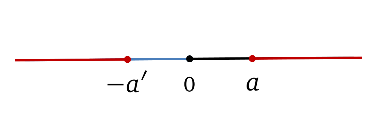
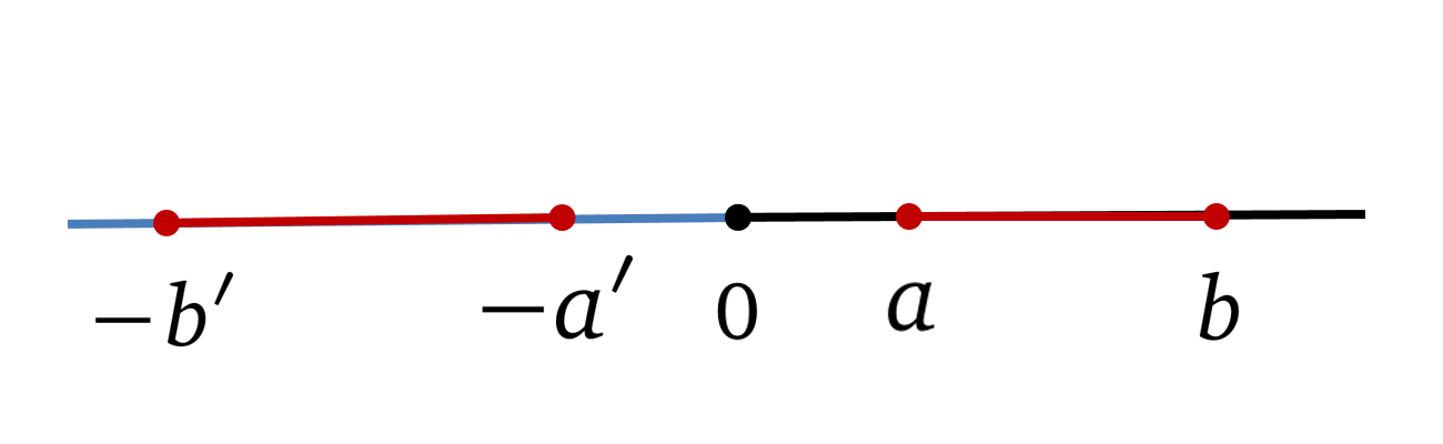
Figure 10: Two configurations in a Weyl-transformed CFT₂ where the island formula may be realized: (left) the entanglement entropy of $\mathcal{R}=[a,\infty)$ in the region $x>0$, admits a minimal saddle by including the island $I=(-\infty,-a^{\prime}]$, (right) $\mathcal{R}=[a,b]$ acquires the island $I=[-b^{\prime},-a^{\prime}]$.

Firstly, let us consider $\mathcal{R}$ to be the semi-infinite region $x>a$ (see the left figure in Fig.10) and apply the Island formula I and (45) to calculate the entanglement entropy. The entanglement entropy calculated by the island formula is given by

$$S_{\mathcal{R}}=\text{min}\left\{\frac{c}{3}\log\frac{a+a^{\prime}}{\delta}-\frac{c}{6}\log\left(\frac{2a^{\prime}}{\delta}\right)+\frac{c}{6}\kappa\right\}\,,$$ (53)

where we have admitted the region $I=(-\infty,-a^{\prime}]$ as the island corresponding to $\mathcal{R}$. The entropy in eq. 53 has a minimal saddle point

$$S_{\mathcal{R}}=\frac{c}{6}\log\left(\frac{2a}{\delta}\right)+\frac{c}{6}\kappa\,,\qquad a^{\prime}=a\,.$$ (54)

This result is smaller than the entanglement entropy in the non-island phase, hence the entanglement island emerges. Note that, the area term $\frac{Area(X)}{4G}$ does not appear since we did not assume a gravitational theory living on the $x<0$ region of the Weyl transformed CFT₂ or the cutoff brane.

Similarly when we consider $\mathcal{R}$ to be an interval $[a,b]$ inside the region $x>0$ and include the corresponding island $I=[-b^{\prime},-a^{\prime}]$ (see the right figure in Fig.10), the Island formula I will give

$$S_{\mathcal{R}}=\text{min}\left\{\frac{c}{3}\log\frac{a+a^{\prime}}{\delta}+\frac{c}{3}\log\frac{b+b^{\prime}}{\delta}-\frac{c}{6}\log\left(\frac{2a^{\prime}}{\delta}\right)-\frac{c}{6}\log\left(\frac{2b^{\prime}}{\delta}\right)+\frac{c}{3}\kappa\right\}\,,$$ (55)

which has the saddle point

$$S_{\mathcal{R}}=\frac{c}{6}\log\left(4\frac{ab}{\delta^{2}}\right)+\frac{c}{3}\kappa\,,\qquad a^{\prime}=a\,,\quad b^{\prime}=b\,.$$ (56)

Then we compare the entanglement entropy (56) in island phase with the one in the non-island phase, which is given by

$$S_{\mathcal{R}}=\frac{c}{3}\log\left(\frac{b-a}{\delta}\right)\,.$$ (57)

We find that when

$$0<a<b\left(1-2\sqrt{e^{2\kappa}+e^{4\kappa}}+2e^{2\kappa}\right)\,,$$ (58)

the entanglement entropy (56) calculated by the island formula is smaller, hence the configuration enters the island phase.

If we set $\kappa=\rho_{0}$, the cutoff brane for the holographic Weyl transformed CFT overlaps with the EoW brane in the AdS/BCFT setup. Obviously, in both of the setups the calculations for the entanglement entropy via the Island formula I are exactly the same. The similarities between these two setups strongly indicate that the Weyl transformed CFT captured the entanglement structure of the BCFT.

One may suspect our application of the island formula to the Weyl transformed CFT as we have not assumed gravitation coupled to the CFT. To justify this application, we provide two prescriptions. The first prescription is to apply the Island formula II, where the emergence of entanglement island comes from the self-encoding property of the system and gravitation is not necessary. We boldly propose that, when we naively apply Island formula I to a (gravitatioanl or non-gravitational) quantum system and get a smaller entanglement entropy than the normal calculation, then the system should be self-encoded. Furthermore, the coding relation should give the same island configuration as the Island formula I. This strong statement can be simplified to be

• Island formula I$\equiv$ Island formula II.

If the Island formula I gives smaller entanglement entropy, then the path integral in the replica manifold will admit smaller saddle point, assuming that additional twist operators are allowed except those settled on the entangling surface. According to the replica wormhole arguments [26, 27], the existence of gravitation makes the additional twist operators possible by allowing wormhole geometries. On the other hand, according to the Island formula II, the additional twist operators are also allowed if the self-encoding property emerges when additional twist operators gives smaller saddle for the replicated path integral. Of course, more evidences are needed to support this strong proposal. If this is true, the Island formula I is not just a special case of the Island formula II, they are indeed equivalent. This indicates that, we can use the Island formula I to diagnose the self-encoding property of a quantum system, which can be either gravitational or non-gravitational. We can also design a quantum system in a lab where entanglement island emerges, see the appendix B.

The second prescription is more conservative. Following the replica wormhole arguments [26, 27], we should at least couple the $x<0$ region to gravity to allow the emergence of entanglement islands. Accordingly, we should change the boundary conditions on the $x<0$ region from the Dirichlet type to the von Neumann type. Eventually we arrive at the familiar system: AdS₂ gravity coupled to a CFT₂ bath. This setup has been discussed in [86], where the choice of the scalar field is a bit different from (46). It is very close to AdS/BCFT setup, and it has been argued in [86] that the AdS₂ gravity coupled to a CFT₂ bath in this setup is equivalent to a BCFT. In this prescription, we can apply the Island formula I with justification. In this case the scalar field not only determines the cutoff scale, but also directly relates to the metric of the field theory. If the gravity on the $x<0$ region admits the AdS₂ metric as a saddle point, then the scalar field characterizing the Weyl transformation, as well as the cutoff configuration, is determined by the gravity rather than given by hand.

In conclusion, for either of the above two prescriptions, the Weyl transformation introduces a finite cutoff configuration, which induces the emergence of entanglement islands according to Island formula I. The Weyl transformation vastly reduces the Hilbert space of the system and wipes out the UV physics in the $x<0$ region. This gives a perfect simulation for the entanglement structure of the AdS/BCFT setup, and explains why the Bekenstein-Hawking entropy is finite and does not depend on the UV cutoff. Nevertheless, the relation between the gravitational renormalization and the Hilbert space reduction is beyond the scope of this paper. Also, how does the self-encoding property explicitly emerge from this reduction is not clear to us. We leave these problems for future investigation.

5 Discussion

In this paper we provide a mechanism for the emergence of the entanglement islands from a purely quantum information perspective. In this mechanism the emergence of islands is a result of certain constraints on the system that reduce the Hilbert space of the entire system properly, such that the degrees of freedom in certain region $I$ are encoded in the state of another subregion $\mathcal{R}$. We show explicitly how the reduction changes the way we compute the reduced density matrix and how the island formula $II$ arises when we compute the entanglement entropy for $\mathcal{R}$. This can also be understood in probability theory in the following way: the constraints that are applied to all the states in the reduced Hilbert space is the information we know before we study the probability distribution for all the possible configurations, hence the entropy we calculate under the constraints can be understood as the conditional entropy (see also [52] for related discussion), which definitely differs from the entropy under no constraints. It seems that this is the only way we can incorporate the island formula $I$ into quantum information theory, so we claimed that, the island formula $I$ is a special case of the island formula $II$. The island phase is a property of the quantum state and the Hilbert space where the state is embedded in, rather than a special property of gravity.

This mechanism sheds new light on our understanding of gravity. We argued that, the effective theory of a gravity should be understand as a curved field theory under certain constraints, such that the Hilbert space is vastly reduced and the self-encoding property appears. We propose that, these constraints are intrinsic for gravity and may originate from the gravitation renormalization process. Although we do not know the details of the reduced Hilbert space, the constraints may result in a finite cutoff scale in the effective field theory. We used a special Weyl transformation to simulate these constraints and show how explicitly the Hilbert space of the holographic CFT₂ is reduced under this Weyl transformation, and how the cutoff scale becomes finite. More interestingly, we show how explicitly the entanglement island emerges under this Weyl transformation. This story reproduces the main features in the AdS/BCFT setup. It will be interesting to consider other Weyl transformations. For example, we can simulate the Wedge holography [87] if we apply the Weyl transformation (46) on both of the $x>0$ region and the $x<0$ region, but with different $\kappa$. Also we may consider the Weyl transformation that optimizes the path-integral [80]. Our new perspective may help us understand the emergence of negative mutual information in that case [81].

In [54], the authors introduced a non-isometric mapping between the effective theory and the fundamental description. Under this non-isometric mapping the dimension of the Hilbert space in the effective theory is tremendously reduced to match the dimension of the Hilbert space of the fundamental description. They claim that in the effective theory, there are large number of null states which vanishes under this mapping. They perform a direct calculation for the reduced density matrix and entanglement entropy for the “reservoir” $\mathcal{R}$ and found that the entropy has two saddles, which is just the expectation from the island formula. We believe that their non-isometric mapping plays a similar role as our Weyl transformation which reduces the Hilbert space and leads to the self-encoding property. On the other hand, there are still important criticisms [36, 37, 38, 39, 40, 41, 42] for the Island formula I which remain to be properly addressed. For example, it was shown in [36] that, the setup where gravity is stopped at the common boundary of the gravity and reservoir will result in massive gravitons (see also [88, 89] for alternative viewpoint). Furthermore in [41] the authors considered a situation in which gravity enters the reservoir while the island does not emerge to rescue unitarity. Also in [42] an inconsistency between Gauss law and the Island formula was pointed out in a theory with long-range gravity. Our Island formula $II$ in non-gravitational systems is definitely free from these criticisms since gravitation is not involved. The self-encoding property of gravity make the Hilbert not factorizable, as was pointed out in [39], but according to our discussion, this is consistent with the island formula. Our new perspective on the Island formula may shed light on properly addressing the above criticisms.

Appendix A The cutoff spheres and their common tangent

The AdS₃ metric in Poincaré coordinates $(t,x,z)$ is given by

$$\differential{s^{2}}=\frac{-\differential{t^{2}}+\differential{x^{2}}+\differential{z^{2}}}{z^{2}}.$$ (59)

In the light-cone coordinates

$$U=\frac{x+t}{2},\quad V=\frac{x-t}{2},\quad\rho=\frac{2}{z^{2}},$$ (60)

the length of the geodesic connecting two spacelike-separated points is[90]

$$L_{\mathrm{AdS}} (U_{1},V_{1},\rho_{1},U_{2},V_{2},\rho_{2})$$

$$=\frac{1}{2}\log\left[\frac{\rho_{2}(\rho_{2}+X)+\rho_{1}(\rho_{2}Y(2\rho_{2}+X)+X)+(\rho_{1}+\rho_{2}\rho_{1}Y)^{2}}{2\rho_{1}\rho_{2}}\right]\,,$$ (61)

where

$$\begin{aligned} Y=&2(U_{1}-U_{2})(V_{1}-V_{2})\,,\\ X=&\sqrt[]{\rho_{1}^{2}+2\rho_{2}\rho_{1}(\rho_{1}Y-1)+(\rho_{2}+\rho_{1}\rho_{2}Y)^{2}}.\end{aligned}$$ (62)

We look for the set of points $(0,x,z)$ whose geodesic distance from a fixed point $(0,x_{0},\delta)$ is a constant $\absolutevalue{\phi(x_{0})}=\log(\frac{2\absolutevalue{x_{0}}}{\delta})-\kappa$. The equation that $x$ and $z$ should satisfy can be obtained straightforwardly by applying eq. 61:

$$\frac{1}{2}\log\left[\frac{\rho_{2}(\rho_{2}+X)+\rho_{1}(\rho_{2}Y(2\rho_{2}+X)+X)+(\rho_{1}+\rho_{2}\rho_{1}Y)^{2}}{2\rho_{1}\rho_{2}}\right]=\log(\frac{2\absolutevalue{x_{0}}}{\delta})-\kappa\,,$$ (63)

which, after taking the limit $\delta\to 0$, can be simplified to be,

$$\left(x-{x_{0}}\right){}^{2}+\left(z-\absolutevalue{x_{0}}e^{-\kappa}\right)^{2}=\absolutevalue{x_{0}}^{2}e^{-2\kappa}\,,$$ (64)

which is a circle at $(x_{0},\absolutevalue{x_{0}}e^{-\kappa})$ with radius $r=\absolutevalue{x_{0}}e^{-\kappa}$.

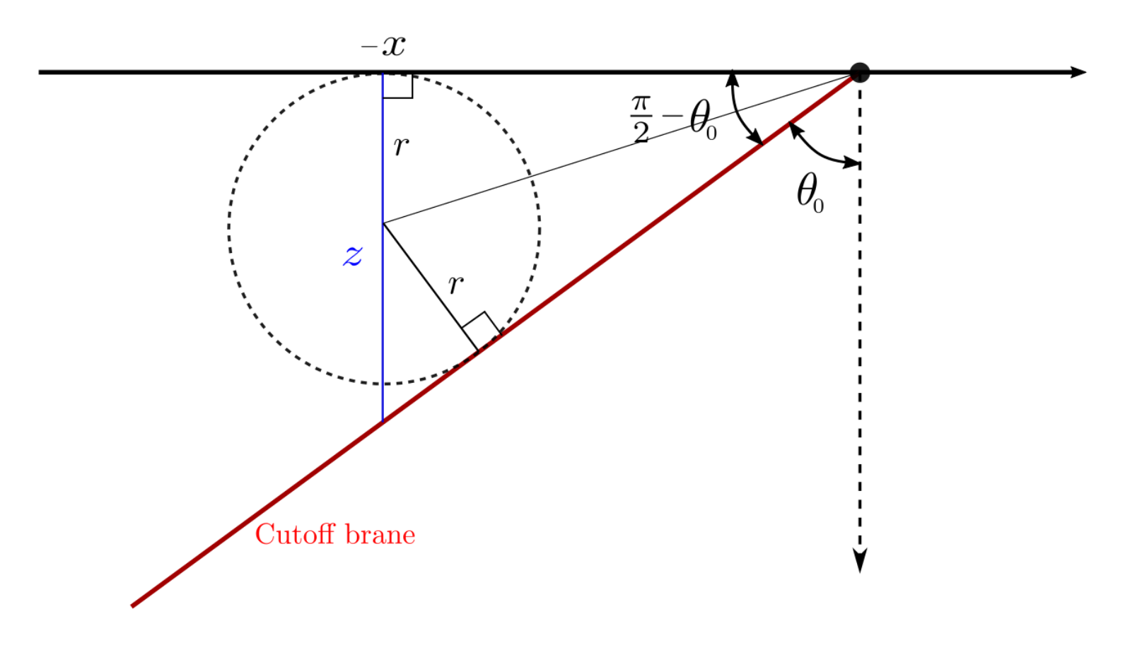
Figure 11: A generic cutoff sphere at $-x$ with radius $r=xe^{-\kappa}$ is centered in the bulk at the point $(x,xe^{-\kappa})$. The tangent from $x=0$ shown by red line acts as a cutoff brane which is equivalent to the EoW brane in the AdS/BCFT scenario.

In fig. 11, a generic cut-off sphere at the point $-x$ (x>0) with radius $r=xe^{-\kappa}$ is depicted. The tangent to the cut-off sphere from $x=0$ is shown by the red line. We may obtain the angle $\theta_{0}$ of the tangent line with the vertical as follows

$$\tan\left(\frac{\pi}{4}-\frac{\theta_{0}}{2}\right)=\frac{r}{|x|}=e^{-\kappa}\,.$$ (65)

Hence, the hyperbolic angle $\rho$ for the tangent line is obtained as

$$\rho=\text{arccosh}\left(\frac{1}{\cos\theta_{0}}\right)=\kappa\,,$$ (66)

which confirms our claim that the cutoff brane obtained from the common tangent line of all the cut-off spheres is equivalent to the end-of-the-world brane in the AdS/BCFT setup.

Appendix B Islands in the lab?

In the main text, we assumed that the Weyl transformed CFT to be holographic such that we have a clear geometric description for the entanglement structure. Nevertheless, we argue that holography is not necessary for the emergence of entanglement islands. For non-holographic CFTs, the entanglement structure may be described by a MERA tensor network [91, 92]. In such scenarios, the tensor network is an analogue of the dual AdS space, and the entanglement entropy is captured by the number of cuts when a path intersects with the tensor network. This path in the tensor network is an analogue to the RT curve [93, 94] and satisfies similar key properties, like it is homologous to the region in the CFT and the number of the cuts should be minimized. Due to such key properties, provided that the two island formulas are equivalent and we can conduct an operation that can adjust the cutoff scale for a certain region like the Weyl transformation, the logic supporting the emergence of islands for the Weyl transformed CFT should also work for non-holographic quantum systems. Such an operation should be understood as eliminating the short distance entanglement inside a region while keeping the long range entanglement between this region and its complement unaffected.

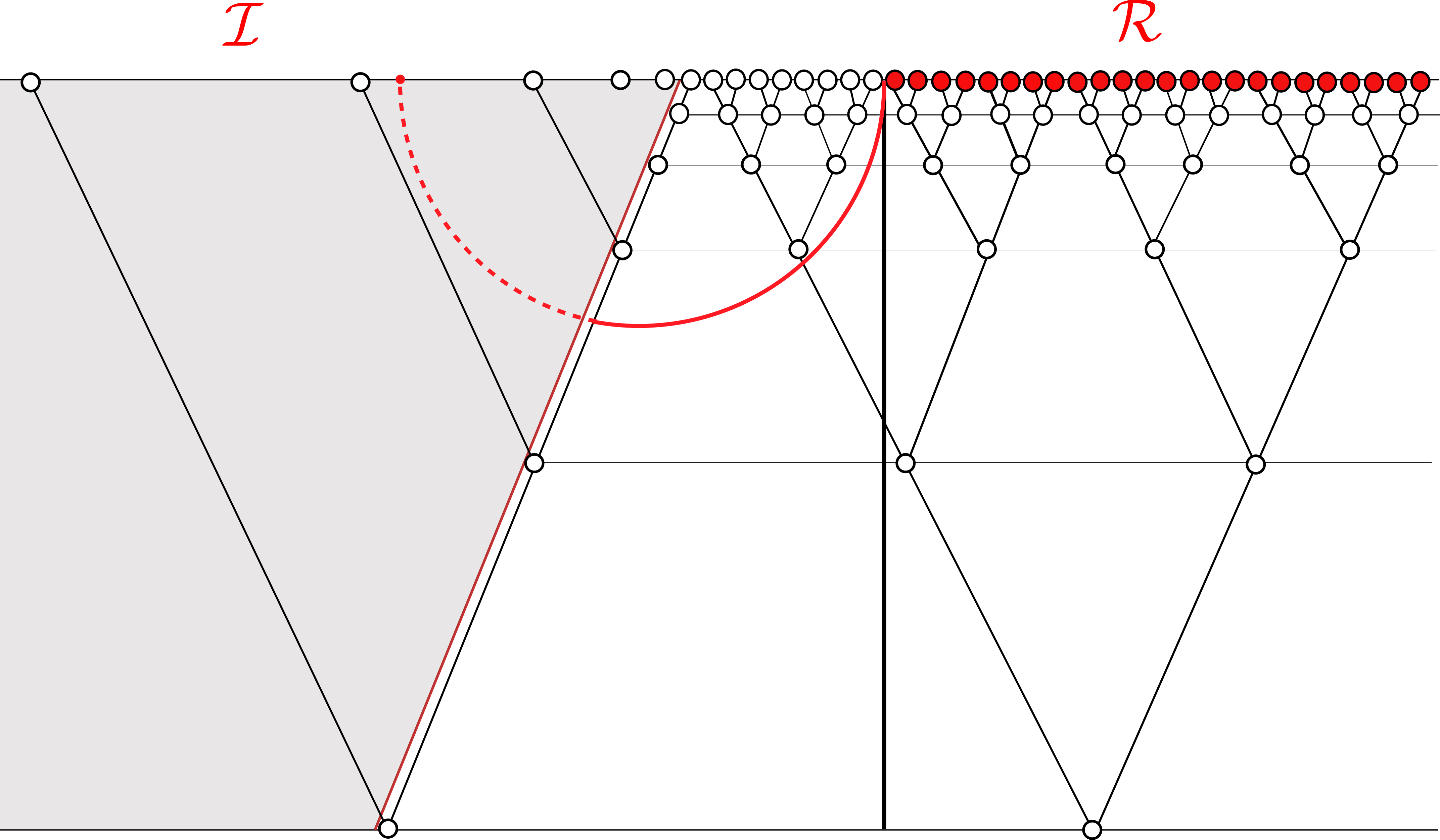
Figure 12: A rough modified MERA tensor network description for the entanglement structure of the Weyl transformed CFT, where islands emerge. The red path clearly has a smaller number of cuts than the black one, hence should be used to evaluate the entanglement entropy of $\mathcal{R}$. The island naturally emerge under the choice of the new path.

We start from a lattice chain where an interacting quantum theory lives and consider the state to be the ground state of the theory. The lattice spacing is settled to be some small constants $\delta$. Then we perform an analogue of the Weyl transformation by adjusting the lattice space for the $x<0$ region. The position dependent lattice spacing $\delta(x)$ controls the cutoff scale. If the lattice spacing $\delta(x)$ increases rapidly enough with $|x|$, then the density of degrees of freedom is vastly reduced and the local short distance entanglement below the scale $\delta(x)$ is eliminated, while the long distance entanglement is almost unaffected. Under such an operation the entanglement structure of the system would roughly be described by the tensor network shown in Fig.12, where a new path homologous to $\mathcal{R}$ emerges with a smaller number of cuts and an island on the left hand side. The new path induces an additional twist operator in the complement of $\mathcal{R}$, hence the entanglement island $I$ emerges. It will be very interesting to construct tensor network models and synthesize lattice models where the special entanglement structure can be (roughly) realized, then explicitly study how the state of $I$ can be encoded in the state of $\mathcal{R}$.

References

- [1] S. W. Hawking, Breakdown of Predictability in Gravitational Collapse, Phys. Rev. D 14, 2460 (1976), 10.1103/PhysRevD.14.2460.
- [2] D. N. Page, Information in black hole radiation, Phys. Rev. Lett. 71, 3743 (1993), 10.1103/PhysRevLett.71.3743, hep-th/9306083.
- [3] D. N. Page, Time Dependence of Hawking Radiation Entropy, JCAP 09, 028 (2013), 10.1088/1475-7516/2013/09/028, 1301.4995.
- [4] S. D. Mathur, The Information paradox: A Pedagogical introduction, Class. Quant. Grav. 26, 224001 (2009), 10.1088/0264-9381/26/22/224001, 0909.1038.
- [5] A. Almheiri, D. Marolf, J. Polchinski and J. Sully, Black Holes: Complementarity or Firewalls?, JHEP 02, 062 (2013), 10.1007/JHEP02(2013)062, 1207.3123.
- [6] J. M. Maldacena, The Large N limit of superconformal field theories and supergravity, Adv. Theor. Math. Phys. 2, 231 (1998), 10.1023/A:1026654312961, hep-th/9711200.
- [7] S. S. Gubser, I. R. Klebanov and A. M. Polyakov, Gauge theory correlators from noncritical string theory, Phys. Lett. B 428, 105 (1998), 10.1016/S0370-2693(98)00377-3, hep-th/9802109.
- [8] E. Witten, Anti-de Sitter space and holography, Adv. Theor. Math. Phys. 2, 253 (1998), 10.4310/ATMP.1998.v2.n2.a2, hep-th/9802150.
- [9] S. Ryu and T. Takayanagi, Holographic derivation of entanglement entropy from AdS/CFT, Phys. Rev. Lett. 96, 181602 (2006), 10.1103/PhysRevLett.96.181602, hep-th/0603001.
- [10] S. Ryu and T. Takayanagi, Aspects of Holographic Entanglement Entropy, JHEP 08, 045 (2006), 10.1088/1126-6708/2006/08/045, hep-th/0605073.
- [11] A. Lewkowycz and J. Maldacena, Generalized gravitational entropy, JHEP 08, 090 (2013), 10.1007/JHEP08(2013)090, 1304.4926.
- [12] T. Faulkner, A. Lewkowycz and J. Maldacena, Quantum corrections to holographic entanglement entropy, JHEP 11, 074 (2013), 10.1007/JHEP11(2013)074, 1307.2892.
- [13] N. Engelhardt and A. C. Wall, Quantum Extremal Surfaces: Holographic Entanglement Entropy beyond the Classical Regime, JHEP 01, 073 (2015), 10.1007/JHEP01(2015)073, 1408.3203.
- [14] A. C. Wall, Maximin Surfaces, and the Strong Subadditivity of the Covariant Holographic Entanglement Entropy, Class. Quant. Grav. 31(22), 225007 (2014), 10.1088/0264-9381/31/22/225007, 1211.3494.
- [15] X. Dong, A. Lewkowycz and M. Rangamani, Deriving covariant holographic entanglement, JHEP 11, 028 (2016), 10.1007/JHEP11(2016)028, 1607.07506.
- [16] C. Akers, N. Engelhardt, G. Penington and M. Usatyuk, Quantum Maximin Surfaces, JHEP 08, 140 (2020), 10.1007/JHEP08(2020)140, 1912.02799.
- [17] X. Dong and A. Lewkowycz, Entropy, Extremality, Euclidean Variations, and the Equations of Motion, JHEP 01, 081 (2018), 10.1007/JHEP01(2018)081, 1705.08453.
- [18] V. E. Hubeny, M. Rangamani and T. Takayanagi, A Covariant holographic entanglement entropy proposal, JHEP 07, 062 (2007), 10.1088/1126-6708/2007/07/062, 0705.0016.
- [19] G. Penington, Entanglement Wedge Reconstruction and the Information Paradox, JHEP 09, 002 (2020), 10.1007/JHEP09(2020)002, 1905.08255.
- [20] A. Almheiri, N. Engelhardt, D. Marolf and H. Maxfield, The entropy of bulk quantum fields and the entanglement wedge of an evaporating black hole, JHEP 12, 063 (2019), 10.1007/JHEP12(2019)063, 1905.08762.
- [21] M. Rozali, J. Sully, M. Van Raamsdonk, C. Waddell and D. Wakeham, Information radiation in BCFT models of black holes, JHEP 05, 004 (2020), 10.1007/JHEP05(2020)004, 1910.12836.
- [22] H. Z. Chen, Z. Fisher, J. Hernandez, R. C. Myers and S.-M. Ruan, Information Flow in Black Hole Evaporation, JHEP 03, 152 (2020), 10.1007/JHEP03(2020)152, 1911.03402.
- [23] A. Almheiri, R. Mahajan, J. Maldacena and Y. Zhao, The Page curve of Hawking radiation from semiclassical geometry, JHEP 03, 149 (2020), 10.1007/JHEP03(2020)149, 1908.10996.
- [24] A. Almheiri, R. Mahajan and J. E. Santos, Entanglement islands in higher dimensions, SciPost Phys. 9(1), 001 (2020), 10.21468/SciPostPhys.9.1.001, 1911.09666.
- [25] A. Almheiri, R. Mahajan and J. Maldacena, Islands outside the horizon (2019), 1910.11077.
- [26] A. Almheiri, T. Hartman, J. Maldacena, E. Shaghoulian and A. Tajdini, Replica Wormholes and the Entropy of Hawking Radiation, JHEP 05, 013 (2020), 10.1007/JHEP05(2020)013, 1911.12333.
- [27] G. Penington, S. H. Shenker, D. Stanford and Z. Yang, Replica wormholes and the black hole interior, JHEP 03, 205 (2022), 10.1007/JHEP03(2022)205, 1911.11977.
- [28] Y. Chen, Pulling Out the Island with Modular Flow, JHEP 03, 033 (2020), 10.1007/JHEP03(2020)033, 1912.02210.
- [29] Y. Chen, X.-L. Qi and P. Zhang, Replica wormhole and information retrieval in the SYK model coupled to Majorana chains, JHEP 06, 121 (2020), 10.1007/JHEP06(2020)121, 2003.13147.
- [30] H. Z. Chen, R. C. Myers, D. Neuenfeld, I. A. Reyes and J. Sandor, Quantum Extremal Islands Made Easy, Part II: Black Holes on the Brane, JHEP 12, 025 (2020), 10.1007/JHEP12(2020)025, 2010.00018.
- [31] J. Hernandez, R. C. Myers and S.-M. Ruan, Quantum extremal islands made easy. Part III. Complexity on the brane, JHEP 02, 173 (2021), 10.1007/JHEP02(2021)173, 2010.16398.
- [32] G. Grimaldi, J. Hernandez and R. C. Myers, Quantum extremal islands made easy. Part IV. Massive black holes on the brane, JHEP 03, 136 (2022), 10.1007/JHEP03(2022)136, 2202.00679.
- [33] I. Akal, Y. Kusuki, N. Shiba, T. Takayanagi and Z. Wei, Entanglement Entropy in a Holographic Moving Mirror and the Page Curve, Phys. Rev. Lett. 126(6), 061604 (2021), 10.1103/PhysRevLett.126.061604, 2011.12005.
- [34] F. Deng, J. Chu and Y. Zhou, Defect extremal surface as the holographic counterpart of Island formula, JHEP 03, 008 (2021), 10.1007/JHEP03(2021)008, 2012.07612.
- [35] T. Anous, M. Meineri, P. Pelliconi and J. Sonner, Sailing past the End of the World and discovering the Island, SciPost Phys. 13(3), 075 (2022), 10.21468/SciPostPhys.13.3.075, 2202.11718.
- [36] H. Geng and A. Karch, Massive islands, JHEP 09, 121 (2020), 10.1007/JHEP09(2020)121, 2006.02438.
- [37] A. Karlsson, Replica wormhole and island incompatibility with monogamy of entanglement (2020), 2007.10523.
- [38] S. Raju, Lessons from the information paradox, Phys. Rept. 943, 2187 (2022), 10.1016/j.physrep.2021.10.001, 2012.05770.
- [39] S. Raju, Failure of the split property in gravity and the information paradox, Class. Quant. Grav. 39(6), 064002 (2022), 10.1088/1361-6382/ac482b, 2110.05470.
- [40] A. Laddha, S. G. Prabhu, S. Raju and P. Shrivastava, The Holographic Nature of Null Infinity, SciPost Phys. 10(2), 041 (2021), 10.21468/SciPostPhys.10.2.041, 2002.02448.
- [41] H. Geng, A. Karch, C. Perez-Pardavila, S. Raju, L. Randall, M. Riojas and S. Shashi, Information Transfer with a Gravitating Bath, SciPost Phys. 10(5), 103 (2021), 10.21468/SciPostPhys.10.5.103, 2012.04671.
- [42] H. Geng, A. Karch, C. Perez-Pardavila, S. Raju, L. Randall, M. Riojas and S. Shashi, Inconsistency of islands in theories with long-range gravity, JHEP 01, 182 (2022), 10.1007/JHEP01(2022)182, 2107.03390.
- [43] M. Alishahiha, A. Faraji Astaneh and A. Naseh, Island in the presence of higher derivative terms, JHEP 02, 035 (2021), 10.1007/JHEP02(2021)035, 2005.08715.
- [44] S. A. Hosseini Mansoori, O. Luongo, S. Mancini, M. Mirjalali, M. Rafiee and A. Tavanfar, Planar black holes in holographic axion gravity: Islands, Page times, and scrambling times, Phys. Rev. D 106(12), 126018 (2022), 10.1103/PhysRevD.106.126018, 2209.00253.
- [45] A. Karch, H. Sun and C. F. Uhlemann, Double holography in string theory, JHEP 10, 012 (2022), 10.1007/JHEP10(2022)012, 2206.11292.
- [46] C. F. Uhlemann, Islands and Page curves in 4d from Type IIB, JHEP 08, 104 (2021), 10.1007/JHEP08(2021)104, 2105.00008.
- [47] C. Krishnan, V. Patil and J. Pereira, Page Curve and the Information Paradox in Flat Space (2020), 2005.02993.
- [48] C. Krishnan, Critical Islands, JHEP 01, 179 (2021), 10.1007/JHEP01(2021)179, 2007.06551.
- [49] K. Ghosh and C. Krishnan, Dirichlet baths and the not-so-fine-grained Page curve, JHEP 08, 119 (2021), 10.1007/JHEP08(2021)119, 2103.17253.
- [50] A. Almheiri, T. Hartman, J. Maldacena, E. Shaghoulian and A. Tajdini, The entropy of Hawking radiation, Rev. Mod. Phys. 93(3), 035002 (2021), 10.1103/RevModPhys.93.035002, 2006.06872.
- [51] R. Bousso, X. Dong, N. Engelhardt, T. Faulkner, T. Hartman, S. H. Shenker and D. Stanford, Snowmass White Paper: Quantum Aspects of Black Holes and the Emergence of Spacetime (2022), 2201.03096.
- [52] R. Renner and J. Wang, The black hole information puzzle and the quantum de Finetti theorem (2021), 2110.14653.
- [53] X. Wang, K. Zhang and J. Wang, What can we learn about islands and state paradox from quantum information theory? (2021), 2107.09228.
- [54] C. Akers, N. Engelhardt, D. Harlow, G. Penington and S. Vardhan, The black hole interior from non-isometric codes and complexity (2022), 2207.06536.
- [55] A. Almheiri and H. W. Lin, The entanglement wedge of unknown couplings, JHEP 08, 062 (2022), 10.1007/JHEP08(2022)062, 2111.06298.
- [56] R. Bousso, B. Freivogel, S. Leichenauer, V. Rosenhaus and C. Zukowski, Null Geodesics, Local CFT Operators and AdS/CFT for Subregions, Phys. Rev. D 88, 064057 (2013), 10.1103/PhysRevD.88.064057, 1209.4641.
- [57] B. Czech, J. L. Karczmarek, F. Nogueira and M. Van Raamsdonk, The Gravity Dual of a Density Matrix, Class. Quant. Grav. 29, 155009 (2012), 10.1088/0264-9381/29/15/155009, 1204.1330.
- [58] M. Headrick, V. E. Hubeny, A. Lawrence and M. Rangamani, Causality & holographic entanglement entropy, JHEP 12, 162 (2014), 10.1007/JHEP12(2014)162, 1408.6300.
- [59] A. Almheiri, X. Dong and D. Harlow, Bulk Locality and Quantum Error Correction in AdS/CFT, JHEP 04, 163 (2015), 10.1007/JHEP04(2015)163, 1411.7041.
- [60] X. Dong, D. Harlow and A. C. Wall, Reconstruction of Bulk Operators within the Entanglement Wedge in Gauge-Gravity Duality, Phys. Rev. Lett. 117(2), 021601 (2016), 10.1103/PhysRevLett.117.021601, 1601.05416.
- [61] D. Harlow, The Ryu–Takayanagi Formula from Quantum Error Correction, Commun. Math. Phys. 354(3), 865 (2017), 10.1007/s00220-017-2904-z, 1607.03901.
- [62] C. Chowdhury, O. Papadoulaki and S. Raju, A physical protocol for observers near the boundary to obtain bulk information in quantum gravity, SciPost Phys. 10(5), 106 (2021), 10.21468/SciPostPhys.10.5.106, 2008.01740.
- [63] C. Chowdhury, V. Godet, O. Papadoulaki and S. Raju, Holography from the Wheeler-DeWitt equation, JHEP 03, 019 (2022), 10.1007/JHEP03(2022)019, 2107.14802.
- [64] G. Dvali and S. N. Solodukhin, Black Hole Entropy and Gravity Cutoff (2008), 0806.3976.
- [65] S. N. Solodukhin, Entanglement entropy of black holes, Living Rev. Rel. 14, 8 (2011), 10.12942/lrr-2011-8, 1104.3712.
- [66] P. Calabrese and J. L. Cardy, Entanglement entropy and quantum field theory, J. Stat. Mech. 0406, P06002 (2004), 10.1088/1742-5468/2004/06/P06002, hep-th/0405152.
- [67] P. Calabrese and J. Cardy, Entanglement entropy and conformal field theory, J. Phys. A 42, 504005 (2009), 10.1088/1751-8113/42/50/504005, 0905.4013.
- [68] H. Casini, M. Huerta and J. A. Rosabal, Remarks on entanglement entropy for gauge fields, Phys. Rev. D 89(8), 085012 (2014), 10.1103/PhysRevD.89.085012, 1312.1183.
- [69] S. Ghosh, R. M. Soni and S. P. Trivedi, On The Entanglement Entropy For Gauge Theories, JHEP 09, 069 (2015), 10.1007/JHEP09(2015)069, 1501.02593.
- [70] L.-Y. Hung and Y. Wan, Revisiting Entanglement Entropy of Lattice Gauge Theories, JHEP 04, 122 (2015), 10.1007/JHEP04(2015)122, 1501.04389.
- [71] S. Hawking, J. M. Maldacena and A. Strominger, de Sitter entropy, quantum entanglement and AdS / CFT, JHEP 05, 001 (2001), 10.1088/1126-6708/2001/05/001, hep-th/0002145.
- [72] G. Dvali, Black Holes and Large N Species Solution to the Hierarchy Problem, Fortsch. Phys. 58, 528 (2010), 10.1002/prop.201000009, 0706.2050.
- [73] L. Susskind and J. Uglum, Black hole entropy in canonical quantum gravity and superstring theory, Phys. Rev. D 50, 2700 (1994), 10.1103/PhysRevD.50.2700, hep-th/9401070.
- [74] T. Jacobson, Black hole entropy and induced gravity (1994), gr-qc/9404039.
- [75] S. N. Solodukhin, The Conical singularity and quantum corrections to entropy of black hole, Phys. Rev. D 51, 609 (1995), 10.1103/PhysRevD.51.609, hep-th/9407001.
- [76] N. D. Birrell and P. C. W. Davies, Quantum Fields in Curved Space, Cambridge Monographs on Mathematical Physics. Cambridge Univ. Press, Cambridge, UK, ISBN 978-0-521-27858-4, 978-0-521-27858-4, 10.1017/CBO9780511622632 (1984).
- [77] S. N. Solodukhin, One loop renormalization of black hole entropy due to nonminimally coupled matter, Phys. Rev. D 52, 7046 (1995), 10.1103/PhysRevD.52.7046, hep-th/9504022.
- [78] T. Takayanagi, Holographic Dual of BCFT, Phys. Rev. Lett. 107, 101602 (2011), 10.1103/PhysRevLett.107.101602, 1105.5165.
- [79] P. Caputa, N. Kundu, M. Miyaji, T. Takayanagi and K. Watanabe, Anti-de Sitter Space from Optimization of Path Integrals in Conformal Field Theories, Phys. Rev. Lett. 119(7), 071602 (2017), 10.1103/PhysRevLett.119.071602, 1703.00456.
- [80] P. Caputa, M. Miyaji, T. Takayanagi and K. Umemoto, Holographic Entanglement of Purification from Conformal Field Theories, Phys. Rev. Lett. 122(11), 111601 (2019), 10.1103/PhysRevLett.122.111601, 1812.05268.
- [81] H. A. Camargo, P. Nandy, Q. Wen and H. Zhong, Balanced partial entanglement and mixed state correlations, SciPost Phys. 12(4), 137 (2022), 10.21468/SciPostPhys.12.4.137, 2201.13362.
- [82] M. Fujita, T. Takayanagi and E. Tonni, Aspects of AdS/BCFT, JHEP 11, 043 (2011), 10.1007/JHEP11(2011)043, 1108.5152.
- [83] J. Sully, M. V. Raamsdonk and D. Wakeham, BCFT entanglement entropy at large central charge and the black hole interior, JHEP 03, 167 (2021), 10.1007/JHEP03(2021)167, 2004.13088.
- [84] B. Swingle, Mutual information and the structure of entanglement in quantum field theory (2010), 1010.4038.
- [85] T. Hartman, Entanglement Entropy at Large Central Charge (2013), 1303.6955.
- [86] K. Suzuki and T. Takayanagi, BCFT and Islands in two dimensions, JHEP 06, 095 (2022), 10.1007/JHEP06(2022)095, 2202.08462.
- [87] I. Akal, Y. Kusuki, T. Takayanagi and Z. Wei, Codimension two holography for wedges, Phys. Rev. D 102(12), 126007 (2020), 10.1103/PhysRevD.102.126007, 2007.06800.
- [88] R.-X. Miao, Massless Entanglement Island in Wedge Holography (2022), 2212.07645.
- [89] R.-X. Miao, Entanglement island and Page curve in wedge holography, JHEP 03, 214 (2023), 10.1007/JHEP03(2023)214, 2301.06285.
- [90] Q. Wen, Towards the generalized gravitational entropy for spacetimes with non-Lorentz invariant duals, JHEP 01, 220 (2019), 10.1007/JHEP01(2019)220, 1810.11756.
- [91] G. Vidal, Entanglement Renormalization, Phys. Rev. Lett. 99(22), 220405 (2007), 10.1103/PhysRevLett.99.220405, cond-mat/0512165.
- [92] G. Vidal, Class of Quantum Many-Body States That Can Be Efficiently Simulated, Phys. Rev. Lett. 101, 110501 (2008), 10.1103/PhysRevLett.101.110501, quant-ph/0610099.
- [93] B. Swingle, Entanglement Renormalization and Holography, Phys. Rev. D 86, 065007 (2012), 10.1103/PhysRevD.86.065007, 0905.1317.
- [94] B. Swingle, Constructing holographic spacetimes using entanglement renormalization (2012), 1209.3304.