Island in the Presence of Higher Derivative Terms

Mohsen Alishahiha^a, Amin Faraji Astaneh^b,c and Ali Naseh^c

^a School of Physics, Institute for Research in Fundamental Sciences (IPM)
P.O. Box 19395-5531, Tehran, Iran
^bDepartment of Physics, Sharif University of Technology, Tehran 14588-89694, Iran
^c School of Particles and Accelerators, Institute for Research in Fundamental Sciences (IPM)
P.O. Box 19395-5531, Tehran, Iran

E-mails: alishah@ipm.ir, faraji@sharif.ir, naseh@ipm.ir

Using extended island formula we compute entanglement entropy of Hawking radiation for black hole solutions of certain gravitational models containing higher derivative terms. To be concrete we consider two different four dimensional models to compute entropy for both asymptotically flat and AdS black holes. One observes that the resultant entropy follows the Page curve, thanks to the contribution of the island, despite the fact that the corresponding gravitational models might be non-unitary.

1 Introdunction

According to Hawking’s computations the black hole’s radiation is thermal [1] which results in black hole information paradox [2]. More precisely, being thermal, it leads to the fact that the entanglement entropy of the radiation grows monotonically. This, in turn, implies that the black hole generates more entropy than it has room for. It is in contrast with the Page’s considerations [3, 4] which propose that the corresponding entropy should decrease after the so called the Page time. This is, indeed, what is required by the unitarity of quantum mechanics.

In the context of black hole physics it was generally believed that in order to explain the Page curve one might need to have a better understanding of microscopic description of black hole degrees of freedom. Nonetheless, recently, it was shown that the Page curve could be described within the semiclassical description of gravity [5, 6, 7, 8, 9], at least in two dimensions.

Indeed motivated by holographic entanglement entropy [10, 11] and introducing the quantum extremal surface [12], a new rule for computing the fine grained black hole entropy is proposed in [7] based on which in order to evaluate the entropy of the radiation one should also consider a possible contribution of an island containing a part of the black hole interior. More precisely, the generalized entropy for a region $R$ is given by [7]

$$S_{\rm gen}={\rm Min}\;\left\{{\rm Ext}\left[\frac{A[\partial I]}{4G_{N}}+S_{\rm vN}(R\cup I)\right]\right\},$$ (1.1)

where $I$ is the island whose boundary area is denoted by $A[\partial I]$ and $S_{\rm vN}(R\cup I)$ is the von Neumann entropy of union of the island and the region $R$. Then the rule is to extremize this expression for any possible island and then take the one that results in the minimum entropy.

For two dimensional Jackiw-Teitelboim gravity [13, 14] the island rule has been derived by making use of replica trick [15, 16]. In this context the island contribution is associated with the contribution of new saddle points in the Euclidean path integral (replica wormholes).

It was then wondering if such a prescription is a particular property of the Jackiw-Teitelboim gravity which is conjectured to provide a gravitational description for SYK model [18, 19] that enjoys a disorder average procedure. Actually, the island rule has been applied for yet another interesting two dimensional gravitational model known as CGHS[20] that admits two dimensional asymptotically flat black holes. It was shown that for this model the entropy follows the Page curve too [21, 22, 23].

The existence of the island for higher dimensions has been investigated in [24]. More recently, the Page curve of asymptotically flat black hole for dimensions greater than two has been studied in [25] (see also [26]). It is then natural to pose the question whether the island rule could be extended for gravitational models containing higher derivative terms. Indeed, this is the aim of the present article to explore this possibility.

To be concrete in this paper we shall consider two different four dimensional gravitational actions containing higher curvature terms. The first model has no cosmological constant so that one has to deal with asymptotically flat black holes, while in the second one there is a negative cosmological constant leading to black hole solutions that are asymptotically AdS. Of course, in this case one has to couple the geometry to a bath where the Hawking radiation may be collected.

By making use of the extended island formula we compute the entanglement entropy of the Hawking radiation and observe that in both cases an island appears at late times resulting in an entropy following the Page curve, despite the fact that both models might be non-unitary. We will back to this point later.

The paper is organized as follows. In the next section we will present the general procedure for evaluating the island formula for entropy in the presence of higher derivative terms. Then we use this formula to compute entanglement entropy for the Hawking radiation for asymptotically flat two sided and one sided back holes in sections three and four, respectively. In section five we will address the same question for four dimensional critical gravity where the corresponding black hole solutions are asymptotically AdS. The last section is devoted to discussions.

2 Island formula for entropy

In this section we would like to extend the island formula for the entropy to the cases in which the gravitational action contains higher derivative terms. Let us consider the following total action

$$I=I_{\rm gravity}+I_{\rm matter},$$ (2.1)

where the action of gravity part may be given by

$$I_{\rm gravity}=\frac{1}{16\pi G_{N}}\int d^{d+1}x\sqrt{g}\,\cal{L}(R_{\mu\rho\nu\sigma})\,.$$ (2.2)

with ${\cal L}$ being a function constructed out of contractions of an arbitrary number of Riemann tensors, and $G_{N}$ is the Newton constant. Moreover, $I_{\rm matter}$ stands for the action of quantum matter field propagating on a classic solution of the gravity part. For the quantum matter field we may consider the action of $N$ scalar fields. In what follows we assume $1\ll N\ll\frac{r_{h}^{d-1}}{G_{N}}$, so that the matter contributions dominate the entanglement entropy, while at the same time the back reaction of the scalar fields on the geometry is negligible. Here $r_{h}$ is the horizon radius of the black hole solution we are considering.

Since the model under consideration has higher derivate terms, a natural proposal for island formula is to replace the area term in the island formula (1.1) with a proper area functional [27]. More precisely, for the gravitational action (2.2) one has

$$S_{\rm gen}={\rm Min}\;\left\{{\rm Ext}\left[S_{\rm gravity}+S_{\rm vN,matter}\right]\right\},$$ (2.3)

with

$$S_{\rm gravity}=\frac{1}{4G_{N}}\int_{\Sigma}d^{d-1}y\sqrt{h}\big{\{}-\frac{\partial{\cal L}}{\partial R_{\mu\rho\nu\sigma}}\varepsilon_{\mu\rho}\varepsilon_{\nu\sigma}+\sum_{\alpha}\left(\frac{\partial^{2}{\cal L}}{\partial R_{\mu_{1}\rho_{1}\nu_{1}\sigma_{1}}\partial R_{\mu_{2}\rho_{2}\nu_{2}\sigma_{2}}}\right)_{\alpha}\frac{2K_{\lambda_{1}\rho_{1}\sigma_{1}}K_{\lambda_{2}\rho_{2}\sigma_{2}}}{q_{\alpha}+1}$$ (2.4)

(2.5)

$$\;\;\;\;\;\;\;\;\;\;\;\;\;\;\times\left[(n_{\mu_{1}\mu_{2}}n_{\nu_{1}\nu_{2}}-\varepsilon_{\mu_{1}\mu_{2}}\varepsilon_{\nu_{1}\nu_{2}})n^{\lambda_{1}\lambda_{2}}+(n_{\mu_{1}\mu_{2}}\varepsilon_{\nu_{1}\nu_{2}}+\varepsilon_{\mu_{1}\mu_{2}}n_{\nu_{1}\nu_{2}})\varepsilon^{\lambda_{1}\lambda_{2}}\right]\bigg{\}}\,.$$ (2.6)

Here in terms of two orthogonal unit vectors $n^{i}_{\mu}$ to the co-dimension two hypersurface $\Sigma$, one has

$$n_{\mu\nu}=n^{i}_{\mu}n^{i}_{\nu}g_{ij},\;\;\;\;\;\;\;\;\;\;\varepsilon_{\mu\nu}=n^{i}_{\mu}n^{j}_{\nu}\varepsilon_{ij}\,,$$ (2.7)

where $\varepsilon_{is}$ is the usual Levi-Civita tensor. For more details and convention see [27].

In this paper, to be more concrete, we will restrict ourselves to four dimensional theories in which the corresponding action containing higher derivative terms may be given as follows

$$I_{\text{gravity}}=\frac{1}{16\pi G_{N}}\int d^{4}x\sqrt{g}\bigg{(}R[g]+\lambda_{1}R^{2}[g]+\lambda_{2}R_{\mu\nu}[g]R^{\mu\nu}[g]+\lambda_{\text{GB}}\hskip 1.42262pt\mathcal{L}_{GB}[g]\bigg{)},$$ (2.8)

where

$$\mathcal{L}_{\text{GB}}[g]=R_{\mu\nu\rho\sigma}[g]R^{\mu\nu\rho\sigma}[g]-4R_{\mu\nu}[g]R^{\mu\nu}[g]+R^{2}[g],$$ (2.9)

Indeed this is the most general four dimensional gravitation action consisting of higher derivative terms up to order of $\mathcal{O}(R^{3})$. The Schwarzschild black hole solution of the model is given by

$$ds^{2}=-f(r)dt^{2}+\frac{dr^{2}}{f(r)}+r^{2}d\Omega^{2},\hskip 28.45274ptf(r)=1-\frac{r_{h}}{r}$$ (2.10)

that is an asymptotically flat black hole solution whose Hawking temperature is $T=\frac{1}{4\pi r_{h}}$. On the other hand by making use of the Wald formula for the entropy one has

$$S_{\rm th}=\frac{\pi}{G_{N}}(r_{h}^{2}+4\lambda_{\rm GB}),$$ (2.11)

that is the thermal entropy of the black hole.

For this model the gravity part appearing in the island formula (2.3) is given by [28, 27].

$$S_{\text{gravity}}=\frac{A[\partial I]}{4G_{N}}+\frac{1}{4G_{N}}\int_{\partial I}\left(2\lambda_{1}R[g]+\lambda_{2}\left[R_{\mu\nu}[g]n^{\mu}_{i}n^{\nu}_{i}-\frac{1}{2}K_{i}K_{i}\right]+2\lambda_{\text{GB}}\hskip 1.42262ptR[\partial I]\right).$$ (2.12)

Here $i=1,2$ denotes two transverse directions to the co-dimension two boundary of island $I$ on which the two unit normal vectors are denoted by $n_{i}^{\mu}$. Moreover, $K_{i}$ is the trace of the second fundamental form $K_{i,\mu\nu}=-h_{\mu}^{\alpha}h_{\nu\beta}\nabla_{\alpha}n_{i}^{\beta}$ where $h_{\mu\nu}=g_{\mu\nu}-n_{i,\mu}n_{i,\nu}$ is the induce metric on $\partial I$.

As for the contribution of the matter field one needs to compute the von Neumann entropy which in four dimensions has the following general form [29]

$$S_{\text{vN,matter}}=\frac{A[\partial I]}{\epsilon^{2}}+\tilde{S}\log{\epsilon}+S_{\text{vN,fin}},$$ (2.13)

where $S_{\text{vN,fin}}$ is the finite part of the entanglement entropy, $\epsilon$ is a UV cutoff and $\tilde{S}=A\hskip 1.42262pt\tilde{S}_{\rm Euler}+C\hskip 1.42262pt\tilde{S}_{\rm Weyl}$ with

$$\tilde{S}_{\rm Euler}=\alpha\int_{\partial I}\hskip 2.84526ptR[{\partial I}],$$ (2.14)

$$\tilde{S}_{\rm Weyl}=-\alpha\int_{\partial I}\hskip 2.84526pt\left(R_{\mu\nu\alpha\beta}[g]n^{\mu}_{i}n^{\nu}_{j}n^{\alpha}_{i}n^{\beta}_{j}-R_{\mu\nu}[g]n^{\mu}_{i}n^{\nu}_{i}+\frac{1}{3}R[g]-\text{Tr}K^{2}+\frac{1}{2}K_{i}K_{i}\right).$$ (2.15)

Here ”$\alpha$” is a finite constant number (see [29]) and $A,C$ are the coefficients of the Euler term and the Weyl square term in 4D conformal anomaly, respectively. These two constants play the role of the central charges in four dimensions which are of order of $N$. On the other hand by making use the Gauss-Godazzi equation,

$$R[g]=R[{\partial I}]-R_{\mu\nu\alpha\beta}[g]n^{\mu}_{i}n^{\nu}_{j}n^{\alpha}_{i}n^{\beta}_{j}+2R_{\mu\nu}[g]n^{\mu}_{i}n^{\nu}_{i}+\text{Tr}K^{2}-K_{i}K_{i},$$ (2.16)

the von Neumann entropy (2.13) associated with the matter field may be simplified as follows

$$S_{\text{vN}}=\frac{A[{\partial I}]}{\epsilon^{2}}+\alpha\int_{\partial I}\left(\frac{2C}{3}R[g]-C\left[R_{\mu\nu}[g]n^{\mu}_{i}n^{\nu}_{i}-\frac{1}{2}K_{i}K_{i}\right]+(A-C)R[{\partial I}]\right)\log{\epsilon}+S_{\text{vN,fin}}.$$ (2.17)

Putting both contributions given by equations (2.12) and (2.17) together, it becomes clear that the UV divergences of von Neumann entropy of the matter field may be absorbed by a renomalization of the Newton constant, as well as the coupling constants of higher derivative terms. More precisely, due to the matter loops the Newton constant will be renormalized as

$$\frac{1}{4G_{N}}\rightarrow\frac{1}{4G_{N}}-\frac{1}{\epsilon^{2}}\,,$$

and this will cancel out the area divergent term in $S_{\text{vN,matter}}$ (see e.g. [30]). In a similar way the log divergent term in $S_{\text{vN,matter}}$ will be dropped out by the corrections which have root in the renormalization of the coupling constants of the higher derivative terms ($\lambda$’s in (2.12)), so although we start with a four dimensional formula for the entropy in its full structure form, we end up with a finite term, $S_{\text{vN,fin}}$ at the end of the day. This term will quantify the mutual information between the regions constructed in radiation part as well as the Island. Since this is very hard to find a universal mutual information in four dimensions we just use the above argument about the propagation of the $s$-modes to estimate the mutual information with a two dimensional formula for which we have a closed form whose universality has already been proved. Putting things together, one finally arrives at

$$S_{\text{gen}}(R)=\text{Min}\bigg{\{}\text{Ext}\bigg{[}\frac{A[\partial I]}{4G_{\text{N,ren}}}$$ (2.18)

$$+\frac{1}{4G_{\text{N,ren}}}\int_{\partial I}\bigg{(}2\lambda_{1,\text{ren}}R[g]+\lambda_{2,\text{ren}}\sum_{i=1}^{2}\left[R_{\mu\nu}[g]n^{\mu}_{i}n^{\nu}_{i}-\frac{1}{2}K_{i}K_{i}\right]+2\lambda_{\text{GB},\text{ren}}\hskip 0.28453ptR[\partial I]\bigg{)}$$ (2.19)

$$\hskip 34.14322pt+S_{\text{vN.fin}}(R\cup I)\bigg{]}\bigg{\}}.$$ (2.20)

This is, indeed, the island formula we will use to compute the entanglement entropy of the Hawking radiation for the four dimensional asymptotically flat black hole (2.10). In fact this should be thought of the semi-classical prescription that computes the fine grained entropy of a black hole when higher derivative terms are also taken into account.

3 Entanglement entropy for two sided black hole

In this section we would like to compute the entanglement entropy of the Hawking radiation for an eternal black hole solution given by (2.10) using the island formula (2.18). To be concrete we consider subregions $R_{+}$ and $R_{-}$ in the radiation part (see figure 1). In an asymptotically flat black hole the radiation region is the part of the spacetime near the null infinity where the gravity is negligible. Practically, we assume that it is above a fictitious boundary located at $r=r_{0}$ as shown in the figure 1. Typically it is few time greater than the radius of the horizon e.g. $r_{0}\sim 3r_{h}$. Therefore with this assumption the radial location of the boundary of our entangling regions denoted by $b_{\pm}$ must be greater than $3r_{h}$.

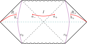
Figure 1: Entanglement regions in the radiation part with the assumption that there is an island inside the black hole. The fictitious boundaries shown by violet lines at $r=r_{0}$ are the regions over which the gravity is negligible that are the radiation regions. At early times assuming that there is an island results in an imaginary solution for the location of island indicating that there is no island at early times and thus the whole contributions come from the matter von Neumann entropy.

We note that the island formula consists of two parts: the gravity part that is associated with a nontrivial quantum extremal surface, island, and the matter von Neumann entropy. A periori, it is not obvious whether or not one should have such an island. Nonetheless to proceed in what follows we will assume that there is a nontrivial island and then we will seek for its location by extremizing the island formula. Note that since the solution we are considering is maximally symmetric the location of a possible island is fixed by its position in $(t,r)$ coordinates. Thus, by extremizing the island formula one obtains a set of algebraic equation.

If the resultant algebraic equations have real solution(s), one would get non-trivial island, otherwise one could conclude that there is, indeed, no island and thus the whole contribution to the entropy comes from the matter von Neumann entropy.

To proceed, let us consider the contribution of the gravity part to the entanglement entropy of the Hawking radiation assuming that there is an island, $I$, whose location is denoted by $a_{\pm}$ in figure 1. As we already mentioned, due to the symmetry of the solution (2.10) the location of island is give by its position in $(t,r)$ coordinates. Therefore the corresponding normal vectors $n_{1}$ and $n_{2}$ associated with the co-dimension two boundary of the island, $\partial I$, are given by

$$n_{1}^{t}=\frac{1}{\sqrt{f(r)}},\hskip 28.45274ptn_{2}^{r}=\sqrt{f(r)}.$$ (3.1)

It is then straightforward to compute the trace of the extrinsic curvature tensors in two normal directions

$$K_{1}=0,\hskip 28.45274ptK_{2}=-\frac{2}{r}\sqrt{f(r)}.$$ (3.2)

We have, now, all ingredients to compute the gravity part of the entropy. Parametrizing the location of the end points of the island by $a_{+}:(t_{a},a)$ and $a_{-}:(-t_{a}+i\frac{\beta}{2},a)$ where $\beta$ is the inverse of the Hawking temperature, one has

$$K_{1}K_{1}=0\ ,\hskip 28.45274ptK_{2}K_{2}=\frac{4}{a^{2}}\left(1-\frac{r_{h}}{a}\right).$$ (3.3)

Moreover taking into account that for the solution (2.10) one has $R_{\mu\nu}[g]=0$ and $R[\partial I]=2/a^{2}$, the gravitational part of the entanglement entropy of the radiation reads

$$S_{\text{gravity}}=\frac{2\pi}{G_{\text{N,ren}}}\bigg{(}a^{2}-2\lambda_{2,\text{ren}}\left(1-\frac{r_{h}}{a}\right)+4\lambda_{\text{GB,ren}}\bigg{)}.$$ (3.4)

Now one should compute the matter von Neumann entropy $S_{\text{vN.fin}}$. Actually, in general, it is not an easy task to compute entanglement entropy for several intervals in four dimensions. It is, however, worth noting that we are, actually, interested in evaluating the entanglement entropy of quantum fields on a maximally symmetric background containing a 2-sphere. Thus we can expand the quantum fields in terms of the spherical harmonics. Reducing to two dimensions one gets a tower of Kaluza-Klein modes whose masses are given by the angular moment along the 2-sphere. On the other hand since we are interested in entangling regions that are far farm each other, one would expect that the main contribution to the von Neumann entropy comes from entanglement between massless modes; the s-wave configuration [5, 25]. In other words, from two dimensional point of view we are throwing away the contributions of massive Kaluza-Klein modes from the entanglement entropy.

In this case, effectively, one might only consider those modes that propagate in two dimensions parametrized by $(t,r)$ coordinates. As a result we could compute the corresponding entanglement entropy between several entangling regions using two dimensional techniques (see for example [31]). To proceed it is useful to work within the Kruskal coordinates

$$U=-\sqrt{\frac{r-r_{h}}{r_{h}}}\hskip 1.42262pte^{-\frac{t-(r-r_{h})}{2r_{h}}},\hskip 14.22636ptV=\sqrt{\frac{r-r_{h}}{r_{h}}}\hskip 1.42262pte^{\frac{t+(r-r_{h})}{2r_{h}}},$$ (3.5)

by which the corresponding two dimensional part of the metric (2.10) reads

$$ds^{2}=-\omega^{-2}dUdV,\hskip 28.45274pt\omega=\sqrt{\frac{r}{4r_{h}^{3}}}\hskip 1.42262pte^{\frac{r-r_{h}}{2r_{h}}}\,.$$ (3.6)

In this two dimensional theory the finite part of the entanglement entropy of the regions $R_{+}$, $R_{-}$ and the island $I$ is given by [31]

$$S_{\rm vN,fin}(R\cup I)=\frac{A}{3}\log\left(\frac{d(a_{+},a_{-})\hskip 1.42262ptd(b_{+},b_{-})\hskip 1.42262ptd(a_{+},b_{+})\hskip 1.42262ptd(a_{-},b_{-})}{d(a_{+},b_{-})\hskip 1.42262ptd(a_{-},b_{+})}\right),$$ (3.7)

where $d(\ell_{1},\ell_{2})$ denotes the geodesic length between two-points $\ell_{1}$ and $\ell_{2}$ that in the above coordinate system reads

$$d(\ell_{1},\ell_{2})=\sqrt{\frac{\big{(}U(\ell_{2})-U(\ell_{1})\big{)}\big{(}V(\ell_{1})-V(\ell_{2})\big{)}}{\omega(\ell_{1})\omega(\ell_{2})}}.$$ (3.8)

To write the above expression for finite part of the entanglement entropy we have used the fact that the whole system represents a pure state and therefore from two dimensional point of view the desired entanglement entropy is the same as that of two disjoint intervals $[b_{-},a_{-}]\cup[a_{+},b_{+}]$.

Using this expression the finite part of the entanglement entropy, equation (3.7) reads [25]

$$S_{\rm vN,fin}(R\cup I)=\frac{A}{6}\log\left[\frac{256(a-r_{h})(b-r_{h})r_{h}^{4}}{ab}\cosh^{2}\frac{t_{a}}{2r_{h}}\cosh^{2}\frac{t_{b}}{2r_{h}}\right]$$ (3.9)

$$\hskip 85.35826pt+\frac{A}{3}\log\left[\frac{\frac{1}{2}\sqrt{\frac{a-r_{h}}{b-r_{h}}}e^{\frac{a-b}{2r_{h}}}+\frac{1}{2}\sqrt{\frac{b-r_{h}}{a-r_{h}}}e^{\frac{b-a}{2r_{h}}}-\cosh\left(\frac{t_{a}-t_{b}}{2r_{h}}\right)}{\frac{1}{2}\sqrt{\frac{a-r_{h}}{b-r_{h}}}e^{\frac{a-b}{2r_{h}}}+\frac{1}{2}\sqrt{\frac{b-r_{h}}{a-r_{h}}}e^{\frac{b-a}{2r_{h}}}+\cosh\left(\frac{t_{a}+t_{b}}{2r_{h}}\right)}\right],$$ (3.10)

which could be further simplified into the following form assuming that $a\approx r_{h}$

$$S_{\rm vN,fin}(R\cup I)=\frac{A}{6}\log\left[\frac{256(a-r_{h})(b-r_{h})r_{h}^{4}}{ab}\cosh^{2}\frac{t_{a}}{2r_{h}}\cosh^{2}\frac{t_{b}}{2r_{h}}\right]$$ (3.11)

$$\hskip 85.35826pt+\frac{A}{3}\log\left[\frac{\frac{1}{2}\sqrt{\frac{b-r_{h}}{a-r_{h}}}e^{\frac{b-a}{2r_{h}}}-\cosh\left(\frac{t_{a}-t_{b}}{2r_{h}}\right)}{\frac{1}{2}\sqrt{\frac{b-r_{h}}{a-r_{h}}}e^{\frac{b-a}{2r_{h}}}+\cosh\left(\frac{t_{a}+t_{b}}{2r_{h}}\right)}\right].$$ (3.12)

Let us first focus on this expression at early times in which $Tt_{a},Tt_{b}\ll 1$. Then, the above expression may be further simplified as follows

$$S_{\rm vN,fin}(R\cup I)=\frac{A}{6}\log\left[\frac{256(a-r_{h})(b-r_{h})r_{h}^{4}}{ab}\cosh^{2}\frac{t_{a}}{2r_{h}}\cosh^{2}\frac{t_{b}}{2r_{h}}\right]$$ (3.13)

$$\hskip 85.35826pt-\frac{4A}{3}\frac{\sqrt{a-r_{h}}}{\sqrt{b-r_{h}}}\hskip 2.84526pte^{\frac{a-b}{2r_{h}}}\cosh\frac{t_{a}}{2r_{h}}\cosh\frac{t_{b}}{2r_{h}}.$$ (3.14)

Plugging the contributions of gravitational part and the above matter part into the generalized entanglement entropy (2.18) one finds

$$S_{\text{gen}}=\frac{2\pi}{G_{\text{N,ren}}}\bigg{(}a^{2}-2\lambda_{2,\text{ren}}\left(1-\frac{r_{h}}{a}\right)+4\lambda_{\text{GB,ren}}\bigg{)}-\frac{4A}{3}\frac{\sqrt{a-r_{h}}}{\sqrt{b-r_{h}}}\hskip 2.84526pte^{\frac{a-b}{2r_{h}}}\cosh\frac{t_{a}}{2r_{h}}\cosh\frac{t_{b}}{2r_{h}}$$ (3.15)

$$\hskip 28.45274pt+\frac{A}{6}\log\left[\frac{256(a-r_{h})(b-r_{h})r_{h}^{4}}{ab}\cosh^{2}\frac{t_{a}}{2r_{h}}\cosh^{2}\frac{t_{b}}{2r_{h}}\right],$$ (3.16)

that should be extremized with respect to the location of the island, i.e. with respect to $a$ and $t_{a}$. Actually from the extremization with respect to $a$ one gets

$$a=r_{h}+\frac{A^{2}G^{2}_{\text{N,ren}}}{36\pi^{2}}\frac{r_{h}^{2}\hskip 1.42262pte^{1-\frac{b}{r_{h}}}}{(b-r_{h})(r_{h}^{2}-\lambda_{2})^{2}}\cosh^{2}\frac{t_{a}}{2r_{h}}\cosh^{2}\frac{t_{b}}{2r_{h}}.$$ (3.17)

Substituting back this value of $a$ into (3.15) and then extremizing with respect $t_{a}$ one finds that the resultant equation does not have a real solution indicating that there is no island at early times.

As a result, in order to compute the entanglement entropy of the Hawking radiation at early times one only needs to consider the contribution of the von Neumann entropy of the matter field. More explicitly, assuming there is no island one has

$$S_{\rm gen}=S_{\rm vN,fin}(R_{+}\cup R_{-})=\frac{A}{3}\log d(b_{+},b_{-})=\frac{A}{6}\log\frac{\big{(}U(b_{-})-U(b_{+})\big{)}\big{(}V(b_{+})-V(b_{-}))}{W(b_{+})W(b_{-}\big{)}},$$ (3.18)

which yields

$$S_{\text{gen}}=\frac{A}{6}\log\left(16r_{h}^{2}\hskip 1.42262pt(\frac{b-r_{h}}{b})\cosh^{2}\frac{t_{b}}{2r_{h}}\right).$$ (3.19)

Note that to write the above expression for entropy we have again used the fact that the whole system is in a pure state and to find the desired entropy one just need to evaluate the entanglement entropy of a signal interval $[b_{-},b_{+}]$ in two dimensions. Form this expression one finds that at early times it exhibits $\mathcal{O}(t^{2})$ growth, while at the late times the entropy grows linearly

$$S_{\text{gen}}\sim\frac{A}{6}\frac{t_{b}}{r_{h}},$$ (3.20)

that leads to information paradox as proposed by Hawking. It is important to note that the above computations were based on an assumption that the no-island scenario remains valid all the way from early to late times. As we will see this is, actually, not the case.

To explore this point better let us redo the same extrimazation procedure when one is approaching the late times. In this case, assuming $Tt_{b},Tt_{a}\gg 1$, the equation (3.11) reduces to

$$S_{\rm vN,fin}(R\cup I)=\frac{A}{6}\log\left(16r_{h}^{4}\hskip 1.42262pt\frac{(b-r_{h})^{2}\hskip 1.42262pte^{\frac{b-a}{r_{h}}}}{ab}\right)-\frac{2A}{3}\sqrt{\frac{a-r_{h}}{b-r_{h}}}\hskip 1.42262pte^{\frac{a-b}{2r_{h}}}\cosh\left(\frac{t_{a}-t_{b}}{2r_{h}}\right).$$ (3.21)

Therefore, in this case the generalized entropy reads

$$S_{\text{gen}} = \frac{2\pi}{G_{\text{N,ren}}}\bigg{(}a^{2}-2\lambda_{2,\text{ren}}\left(1-\frac{r_{h}}{a}\right)+4\lambda_{\text{GB,ren}}\bigg{)}+\frac{A}{6}\log\left(16r_{h}^{4}\hskip 1.42262pt\frac{(b-r_{h})^{2}\hskip 1.42262pte^{\frac{b-a}{r_{h}}}}{ab}\right)$$ (3.24)

$$-\frac{2A}{3}\sqrt{\frac{a-r_{h}}{b-r_{h}}}\hskip 1.42262pte^{\frac{a-b}{2r_{h}}}\cosh\left(\frac{t_{a}-t_{b}}{2r_{h}}\right).$$

From the exterimazation of the generalized entropy one gets

$$\frac{\partial S_{\text{gen}}}{\partial a}=-\frac{A\hskip 1.42262pte^{\frac{r_{h}-b}{2r_{h}}}}{3\sqrt{b-r_{h}}}\cosh\left(\frac{t_{a}-t_{b}}{2r_{h}}\right)\frac{1}{\sqrt{a-r_{h}}}+\frac{12\pi(r_{h}^{2}-\lambda_{2})-A\hskip 1.42262ptG_{\text{N,ren}}}{3r_{h}G_{\text{N,ren}}}+\mathcal{O}(\sqrt{a-r_{h}})=0,$$ (3.25)

that may be solved to find

$$a=r_{h}+\frac{A^{2}r_{h}^{2}\hskip 1.42262ptG_{\text{N,ren}}^{2}}{144\pi^{2}(r_{h}^{2}-\lambda_{2})^{2}}\frac{e^{\frac{r_{h}-b}{r_{h}}}}{(b-r_{h})}\cosh^{2}\left(\frac{t_{a}-t_{b}}{2r_{h}}\right).$$ (3.26)

Here we have used the fact that at leading order one has $12\pi(r_{h}^{2}-\lambda_{2})-A\hskip 1.42262ptG_{\text{N,ren}}\approx 12\pi(r_{h}^{2}-\lambda_{2})$. Substituting the above value of $a$ in (3.24) and extremizing the result with respect to $t_{a}$ one finds that $t_{a}=t_{b}$ is a solution. Thus, one gets nontrivial real solution for the parameters of island indicating that the island shows up at late times when $Tt_{b}\gg 1$. Actually for this solution the generalized entropy (3.24) at late times reads

$$S_{\text{gen}}=2S_{\text{th}}+\frac{A}{6}\log\left(16r_{h}^{3}\hskip 1.42262pt\frac{(b-r_{h})^{2}}{b}\hskip 1.42262pte^{\frac{(b-r_{h})}{r_{h}}}\right)+\mathcal{O}(G_{\text{N,ren}}),$$ (3.27)

where $S_{\rm th}$ is black hole thermal entropy (2.11). It is also worth noting that the contribution of $\lambda_{2}$ term appears in order $G^{2}_{\text{N,ren}}$. From this result it is then clear that the appearance of the island results in the saturation of entanglement entropy at late times in agreement with Page’s proposal.

It is also possible to estimate the time when the entropy stops growing that is known as the Page time. Indeed, this can be done by equating the entropy growth without island (3.19) with the saturation value at late times. Doing so, one arrives at

$$\log\left(\cosh\frac{t_{\rm Page}}{2r_{h}}\right)=\frac{6S_{\text{th}}}{A}+\frac{1}{2}\log\left(r_{h}(b-r_{h})\hskip 1.42262pte^{\frac{(b-r_{h})}{r_{h}}}\right).$$ (3.28)

Tending to the late time limit $Tt_{b}\gg 1$, the above equation may be simplified as follows

$$t_{\rm Page}=\frac{12S_{\text{th}}}{A}\,r_{h}+r_{h}\,\log\left(r_{h}(b-r_{h})\hskip 1.42262pte^{\frac{(b-r_{h})}{r_{h}}}\right).$$ (3.29)

4 Entanglement entropy for one sided black hole

In this section we would like to study entanglement entropy of the Hawking radiation of an asymptotically flat one sided black hole when the corresponding gravitational action contains higher curvature terms. We will consider an entangling region, $R$, in the radiation part of the black hole that is the part near null infinity behind a fictitious boundary over which the gravity is negligible (see figure 2).

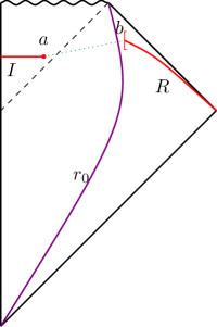
Figure 2: Entanglement regions in the radiation part with the assumption that there is an island inside the black hole. The fictitious boundary shown by violet lines at $r=r_{0}$ specifies the region over which the gravity is negligible, i.e. the radiation region.

Actually the aim is to evaluate the island formula for this configuration. To do so, one needs to compute the generalized entropy assuming that there is an island whose location can be obtained by extreminzing the generalized entropy (2.18). It is important to note that while in two sided black hole the position of the island was outside the horizon, in the present case it is believed that the island is located inside the event horizon [5, 6, 7, 8]. Having this point in mind the gravity contribution to the generalized entropy is found to be

$$S_{\text{gravity}}=\frac{\pi}{G_{\text{N,ren}}}\bigg{(}a^{2}+2\lambda_{2,\text{ren}}\left(1-\frac{r_{h}}{a}\right)+4\lambda_{\text{GB,ren}}\bigg{)}.$$ (4.1)

To find the von Neumann entropy of the matter part, following the procedure we used in the previous section, one may consider entanglement entropy of a two dimensional space given by the metric (3.6). Of course, since the black hole and radiation union is in a pure state, in order to compute the entanglement entropy of radiation and island one just needs to compute the entanglement entropy of an interval $[a,b]$ in two dimensions that is given by

$$S_{\rm vN,fin}=\frac{A}{3}\log d(a,b)$$ (4.2)

where $d(a,b)$ is the geodesic distance between $a$ and $b$ as depicted in the figure 2. To compute the corresponding distance one should use the equation (3.8). It is, however, important to note that since the island is located behind the horizon one should properly define the Kruskal coordinates in this case. More precisely one has

$$U=-e^{-\frac{t-r^{*}}{2r_{h}}},\hskip 28.45274ptV=e^{\frac{t+r^{*}}{2r_{h}}},\hskip 28.45274pt\text{outside the horizon},$$ (4.3)

$$U=e^{-\frac{t-r^{*}}{2r_{h}}},\hskip 28.45274ptV=e^{\frac{t+r^{*}}{2r_{h}}},\hskip 39.83368pt\text{inside the horizon},$$ (4.4)

where the tortoise coordinate, $r^{*}$, is given by

$$r^{*}=r-r_{h}+r_{h}\log\left(\frac{\mid r-r_{h}\mid}{r_{h}}\right).$$ (4.5)

By making use of this notation and utilizing the equation (3.8) one finds

$$S_{\text{vN,fin}} = \frac{A}{6}\log\bigg{[}(a-r_{h})e^{\frac{a-b}{2r_{h}}}+(b-r_{h})e^{\frac{b-a}{2r_{h}}}-2\sqrt{(b-r_{h})(r_{h}-a)}\sinh\left(\frac{t_{a}-t_{b}}{2r_{h}}\right)\bigg{]}$$ (4.7)

$$+\frac{A}{6}\log\bigg{[}\frac{4r_{h}^{2}}{\sqrt{ab}}\bigg{]}$$

To find the location of the island and then the entanglement entropy of the radiation one needs to extremize the generalized entropy with respect to the location of the island. Indeed extremizing the generalized entropy with respect to $a$,

$$\frac{\partial S_{\text{gen}}}{\partial a}=\frac{\partial}{\partial a}\left(S_{\text{gravity}}+S_{\text{vN,fin}}\right)=0,$$ (4.8)

and defining $X=\sqrt{\frac{r_{h}-a}{r_{h}}}$ one arrives at

$$\frac{12\pi(r_{h}^{2}+\lambda_{2,\text{ren}})-AG_{\text{N,ren}}}{G_{\text{N,ren}}}+\frac{r_{h}A}{(b-r_{h})}\left(e^{\frac{r_{h}-b}{r_{h}}}\cosh\left(\frac{t_{a}-t_{b}}{r_{h}}\right)+e^{\frac{r_{h}-b}{2r_{h}}}\sqrt{\frac{b-r_{h}}{r_{h}}}\hskip 2.84526pt\frac{\sinh\left(\frac{t_{a}-t_{b}}{2r_{h}}\right)}{X}\right)$$ (4.9)

$$\hskip 56.9055pt+\mathcal{O}\bigg{(}X\sinh\left(\frac{t_{a}-t_{b}}{2r_{h}}\right)\bigg{)}=0.$$ (4.10)

It is easy to see that at early times when $t_{a}\sim t_{b}$ and $Tt_{b}\ll 1$ the above equation has no solution and therefore one may conclude that at early times there is no island. Thus the whole contribution to the generalized entropy comes from the matter von Neumann entropy. More precisely, in this case one gets

$$S_{\text{gen}}=\frac{A}{6}\log\bigg{[}\frac{4r_{h}^{2}}{\sqrt{b}}\bigg{(}(b-r_{h})e^{\frac{b}{2r_{h}}}-r_{h}e^{\frac{-b}{2r_{h}}}+2\sqrt{(b-r_{h})r_{h}}\sinh(\frac{t_{b}}{2r_{h}})\bigg{)}\bigg{]},$$ (4.11)

that results in the following linear growth at early times

$$S_{\text{gen}}\sim\frac{A}{6}\frac{\sqrt{(b-r_{h})r_{h}}}{r_{h}\left((b-r_{h})e^{\frac{b}{2r_{h}}}-r_{h}e^{\frac{-b}{2r_{h}}}\right)}\hskip 2.84526ptt_{b}\,.$$ (4.12)

Assuming to have no island all the time from early to late times one observes that the entropy increases monotonically, that is consistent with Hawking’s proposal. Of course this is not the case as we will see.

Indeed at late times when $Tt_{b}\gg 1$ the equation (4.9) admits a solution that is given by

$$X=-\frac{A\hskip 1.42262ptG_{\text{N,ren}}\hskip 2.84526pte^{\frac{r_{h}-b}{2r_{h}}}\hskip 1.42262pt\hskip 2.84526pt\sqrt{r_{h}\big{(}b-r_{h}\big{)}}\sinh\left(\frac{t_{a}-t_{b}}{2r_{h}}\right)}{\bigg{(}\big{(}b-r_{h}\big{)}\big{(}12\pi r_{h}^{2}+12\pi\lambda_{2,\text{ren}}-AG_{\text{N,ren}}\big{)}+AG_{\text{N,ren}}\hskip 1.42262pte^{1-\frac{b}{r_{h}}}r_{h}\cosh\left(\frac{t_{a}-t_{b}}{r_{h}}\right)\bigg{)}}.$$ (4.13)

Note that since by definition the quantity $X$ is a positive number, the above expression leads to a solution if $t_{a}<t_{b}$. In other words the location of the island should be in the past of the location of the entangling region $R$. Moreover, from the extremization with respect to $t_{a}$ one finds that

$$\frac{\partial S_{\text{gen}}}{\partial t_{a}}=\frac{A\hskip 1.42262ptG_{\text{N,ren}}\hskip 2.84526pte^{\frac{b}{r_{h}}}}{(b-r_{h})(r_{h}^{2}+\lambda_{2,\text{ren}})}\hskip 1.42262pt\sinh\left(\frac{t_{a}-t_{b}}{r_{h}}\right)$$ (4.14)

$$\times\left(\big{(}b-r_{h}\big{)}\big{(}AG_{\text{N,ren}}+12\pi(r_{h}^{2}+\lambda_{2,\text{ren}})\big{)}+A\hskip 1.42262ptG_{\text{N,ren}}e^{1-\frac{b}{r_{h}}}r_{h}\big{(}1-2\cosh\left(\frac{t_{a}-t_{b}}{r_{h}}\right)\big{)}\right)=0,$$

which can be solved to find (note that $t_{a}<t_{b}$)

$$t_{a}=t_{b}-r_{h}\log S_{\text{th}}-r_{h}\log\left(\frac{12\hskip 1.42262pte^{\frac{b}{r_{h}}-1}(b-r_{h})(r_{h}^{2}+\lambda_{2,\text{ren}})}{A\hskip 1.42262ptr_{h}(r_{h}^{2}+\lambda_{\text{GB,ren}})}\right)+\mathcal{O}(G_{\text{N,ren}}).$$ (4.15)

By making use of the definition of the tortoise coordinates the above equation may be recast into the following form

$$v(a,t_{a})-v(b,t_{b})\sim-r_{h}\log S_{\text{th}}+\mathcal{O}(G^{0}_{\text{N,ren}})\sim-\frac{t_{\text{scr}}}{2},$$ (4.16)

where $v=t+r^{*}$ and $t_{\text{scr}}$ is the scrambling time. This is, indeed, a realization of the Hayden-Preskill decoding criterion [32]. Namely, if one throws a quantum q-bit into the black hole after the Page time, it can be decoded from the Hawking radiation just after waiting for a time of order of the scrambling time.

Finally using this result one may find the generalized entropy at late times when both contributions of island and matter field should be taken into account

$$S_{\text{gen}}=S_{\text{th}}-\frac{A}{12}\left(1-\log\bigg{[}\frac{16e^{\frac{b}{r_{h}}}(b-r_{h})^{2}r_{h}^{3}}{b}\bigg{]}\right)+\mathcal{O}(G_{\text{N,ren}}).$$ (4.17)

To conclude this section we note that although at early times one has a linear growth, the island comes to rescue the unitarity at late times in agreement with the Page curve. In the present case the Page time at leading order is

$$t_{\rm Page}\sim\frac{6S_{\rm th}}{A}r_{h}.$$ (4.18)

5 Page curve for critical gravity

In this section we will explore the behavior of the Page curve for the black hole solutions of yet another interesting gravitational theory containing higher derivative terms. The model we will be considering is “critical gravity” of which the action in four dimensions is [33]

$$I_{\rm critical}=\frac{1}{16\pi G}\int_{\mathcal{M}}d^{4}x\sqrt{-g}\left[R-2\Lambda-\frac{1}{m^{2}}\left(R^{\mu\nu}R_{\mu\nu}-\frac{1}{3}R^{2}\right)\right],$$ (5.1)

where $m$ is a dimensionful parameter. This model admits several solutions including AdS and AdS black holes with radius $\ell^{2}=-\frac{3}{\Lambda}$. It is known that at the critical point where $m^{2}=\frac{8}{\ell^{2}}$ the model degenerates yielding to a log-gravity [34]. Of course in what follows we will study the model away from the critical point, i.e. $m^{2}\neq\frac{8}{\ell^{2}}$.

It is easy to see that the equations of motion obtained from the action (5.1) admits the AdS-Schwarzschild black hole whose metric may be written as follows

$$ds^{2}=\frac{dr^{2}}{f(r)}-f(r)dt^{2}+r^{2}d\Omega^{2}_{2},\;\;\;\;\;\;\;\;\;\;f(r)=\frac{r^{2}}{\ell^{2}}+1-\frac{4GM}{r}.$$ (5.2)

where $M$ is a parameter of the solution (not the physical mass).

For our purpose one needs to couple the above gravitational model to a quantum field that propagate in the above geometry. It is important to note that unlike the solutions we have considered in the previous section, the above metric represents a geometry that is asymptotically AdS. The main difference between asymptotically AdS and asymptotically flat black holes is that, in the former case one usually has reflecting boundary condition on bulk fields at the boundary of spacetime. This will eventually cause the termination of the black hole evaporation due to the equilibrium between the emission and the absorption processes.

To overcome this problem and to have a fully evaporating system, following [5, 6], one should impose transparent boundary condition for the matter field while the boundary condition for the gravitational field remains unchanged. In other words, one should couple the gravitational theory to an external bath constructed of the same quantum matter field propagating in the flat space. So that the bath is a flat spacetime with no gravity where the Hawking radiation could be collected. Therefore altogether we have a system consisting of gravity confined in the AdS geometry and a quantum field that propagate both in AdS and flat spaces with transparent boundary condition at the boundary of the AdS geometry. For quantum matter field one may take the action of $N$ scalar fields, see figure 3.

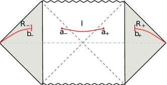
Figure 3: The AdS black hole+Bath system. The bath (colored region) plays the role of the environment around the evaporating black hole. This is necessary to include this environment since the boundary of AdS is reflecting and as a result of that the evaporation will be terminated at some point due to the expected equilibrium between the emission and the absorption processes.

Here the main subtlety is the way the boundary conditions should be imposed so that the whole system (gravity+bath) becomes a consistent model. The corresponding procedure for two dimensional Jackiw-Teitelboim gravity has been carefully worked out in the literature (see e.eg [5, 6, 7, 8]), though its generalization to higher dimensions has not been fully studied yet. Nonetheless in general one would expect that the similar analysis could be done for higher dimensions too.

As far as the gravitational part of the island formula is concerned, it is straightforward to evaluate the corresponding contribution in arbitrary dimensions, though for the matter field it is crucial to have the proper conditions under which the bath is connected to the asymptotic AdS boundary. Motivated by the results of the previous section we note that since the main contribution to the entanglement entropy comes from the s-wave modes of the quantum field, one may effectively work within a two dimensional theory obtained by dimensional reduction from the original four dimensional metric. Therefore one would expect that the same boundary conditions as those in two dimensions may be used here. Actually this is the fact we assume in what follows and accordingly we will use the same procedure as before to compute the finite part of the entanglement entropy.

For a technical simplicity reason in what follows we will consider the case where the radius of curvature is much larger than the radius of horizon so that we could essentially work with a black brane solution whose metric is the same as that in (5.2) with

$$f(r)=\frac{r^{2}}{\ell^{2}}\left(1-\frac{r_{h}^{3}}{r^{3}}\right).$$ (5.3)

It is then easy to evaluate the contribution of gravitational part to the island formula. Actually by making use of the fact that in the present case one has

$$K^{1}=0,\hskip 28.45274ptK^{2}=\frac{2}{r}\sqrt{f(r)},\hskip 28.45274ptR[g]=-\frac{12}{\ell^{2}},\hskip 28.45274pt\sum_{i}R_{\mu\nu}n_{i}^{\mu}n_{i}^{\nu}=0,$$ (5.4)

the gravitational part reads

$$S_{\text{gravity}}=\frac{V_{2}}{2G_{\text{N,ren}}}\hskip 2.84526pt\frac{a^{2}}{\ell^{2}}\left(1-\frac{8}{\ell^{2}m^{2}}+\frac{2}{\ell^{2}m^{2}}(1-\frac{r_{h}^{3}}{a^{3}})\right),$$ (5.5)

where $V_{2}$ is the regularized volume of two dimensional transverse space. As for the matter part, using the Kruskal coordinate

$$U=-e^{-\frac{\beta}{2\pi}(t-r^{*})},\hskip 28.45274ptV=e^{\frac{\beta}{2\pi}(t+r^{*})}$$ (5.6)

the corresponding reduced two dimensional metric is

$$ds^{2}=-\omega^{-2}{dU\hskip 1.42262ptdV},\hskip 42.67912pt\omega=\left(\frac{4\pi^{2}e^{\frac{4\pi r^{*}}{\beta}}}{\beta^{2}f(r)}\right)^{\frac{1}{2}},$$ (5.7)

where $\beta=\frac{4\pi}{f^{\prime}(r_{h})}$ is the inverse of the Hawking temperature and $r^{*}=\int dr/f(r)$ is the tortoise coordinate. Then the finite part of the entanglement entropy will be still obtained from the equation (3.7). It is, however, important to note that in order to compute the geodesic distances one should keep in mind that the whole system (BH+bath) should parametrized with the same coordinate system as above, thought in the bath one should set $f(r)=1$. This technical procedure guarantees that we are dealing with a state that is the Minkowski vacuum in the whole system.

Going through the same computations as those in the section three one finds that at early times, $Tt_{b}\ll 1$, there is no island and the whole contribution to the generalized entropy comes from the matter part. Assuming that there is no island at all, the corresponding generalized entropy becomes

$$S_{\text{gen}}=\frac{A}{3}\log{d(b_{-},b_{+})}=\frac{A}{6}\log\left(\frac{\beta^{2}}{\pi^{2}}\cosh^{2}\left(\frac{2\pi t_{b}}{\beta}\right)\right),$$ (5.8)

that at early times results in $S_{\rm gen}\sim{\rm const.}+\frac{2\pi^{2}A}{3\beta^{2}}\hskip 1.42262ptt_{b}^{2}$, whereas at late times where it keeps growing linearly as follows

$$S_{\text{gen}}\sim\frac{2\pi A}{3\beta}\hskip 2.84526ptt_{b}.$$ (5.9)

On the other hand assuming to have an island at late times one would have to extremize the generalized entropy when both the gravitational part and matter entanglement entropy are taken into count. In this case using the equation (3.7) one arrives at

$$S_{\text{vN,fin}}=-\frac{4\pi A}{3\beta}\big{(}t_{a}+t_{b}\big{)}+\frac{A}{3}\log\left(\frac{\beta^{2}}{4\pi^{2}}\sqrt{f(a)}\hskip 2.84526pt(1+e^{\frac{4\pi t_{a}}{\beta}})(1+e^{\frac{4\pi t_{b}}{\beta}})\right)$$ (5.10)

$$\hskip 28.45274pt-\frac{A}{3}\log\left(\frac{\bigg{(}e^{\frac{2\pi}{\beta}\big{(}t_{a}+r^{*}(a)\big{)}}+e^{\frac{2\pi}{\beta}\big{(}-t_{b}+b\big{)}}\bigg{)}\bigg{(}e^{\frac{2\pi}{\beta}\big{(}-t_{a}+r^{*}(a)\big{)}}+e^{\frac{2\pi}{\beta}\big{(}t_{b}+b\big{)}}\bigg{)}}{\bigg{(}e^{\frac{2\pi}{\beta}\big{(}t_{b}+r^{*}(a)\big{)}}-e^{\frac{2\pi}{\beta}\big{(}t_{a}+b\big{)}}\bigg{)}\bigg{(}e^{\frac{2\pi}{\beta}\big{(}t_{a}+r^{*}(a)\big{)}}-e^{\frac{2\pi}{\beta}\big{(}t_{b}+b\big{)}}\bigg{)}}\right),$$ (5.11)

which at late times, $t_{a},t_{b}\gg\beta$, reads

$$S_{\text{vN,fin}}=-\frac{2\pi A}{3\beta}\bigg{(}t_{a}+t_{b}+r^{*}(a)+b\bigg{)}+\frac{A}{3}\log\left(\frac{\beta^{2}\sqrt{f(a)}}{4\pi^{2}}\right)$$ (5.12)

$$+\frac{A}{3}\log\bigg{(}\big{(}e^{\frac{2\pi}{\beta}\big{(}t_{b}+b\big{)}}-e^{\frac{2\pi}{\beta}\big{(}t_{a}+r^{*}(a)\big{)}}\big{)}\big{(}e^{\frac{2\pi}{\beta}\big{(}t_{a}+b\big{)}}-e^{\frac{2\pi}{\beta}\big{(}t_{b}+r^{*}(a)\big{)}}\big{)}\bigg{)}.$$ (5.13)

Therefore one has to extremize the following expression of the generalized entropy

$$S_{\rm gen} = \frac{V_{2}}{2G_{\text{N,ren}}}\hskip 2.84526pt\frac{a^{2}}{\ell^{2}}\left(1-\frac{8}{\ell^{2}m^{2}}+\frac{2}{\ell^{2}m^{2}}(1-\frac{r_{h}^{3}}{a^{3}})\right)\hskip 2.84526pt-\frac{2\pi A}{3\beta}\bigg{(}t_{a}+t_{b}+r^{*}(a)+b\bigg{)}$$ (5.15)

$$+\frac{A}{3}\log\left(\frac{\beta^{2}\sqrt{f(a)}}{4\pi^{2}}\right)+\frac{A}{3}\log\bigg{(}\big{(}e^{\frac{2\pi}{\beta}\big{(}t_{b}+b\big{)}}-e^{\frac{2\pi}{\beta}\big{(}t_{a}+r^{*}(a)\big{)}}\big{)}\big{(}e^{\frac{2\pi}{\beta}\big{(}t_{a}+b\big{)}}-e^{\frac{2\pi}{\beta}\big{(}t_{b}+r^{*}(a)\big{)}}\big{)}\bigg{)}.$$

Actually It is straightforward to show that at late times the equation

$$\frac{\partial S_{\text{gen}}}{\partial t_{a}}=0,$$ (5.16)

implies $t_{a}=t_{b}$, while from the equation

$$\frac{\partial S_{\text{gen}}}{\partial a}=0,$$ (5.17)

one finds

$$a=r_{h}+\frac{A^{2}\ell^{8}m^{4}G^{2}_{\text{N,ren}}}{9\sqrt{3}\hskip 1.42262ptr_{h}^{3}\left(\ell^{2}m^{2}-5\right)^{2}V_{2}^{2}}\hskip 2.84526pte^{\frac{\pi}{\sqrt{3}}-\frac{3b\hskip 1.42262ptr_{h}}{l^{2}}}.$$ (5.18)

Plugging this result into the expression of generalized entropy one arrives at

$$S_{\text{gen}}=\frac{V_{2}r_{h}^{2}}{2\ell^{2}G_{\text{N,ren}}}\left(1-\frac{8}{\ell^{2}m^{2}}\right)+\frac{A}{6}\left(\frac{3b\hskip 1.42262ptr_{h}}{\ell^{2}}-\frac{\pi}{\sqrt{3}}+\log(\frac{16\ell^{6}}{9\sqrt{3}r_{h}^{2}})\right)+\mathcal{O}(G_{\text{N,ren}}).$$ (5.19)

that is

$$S_{\text{gen}}=2S_{\text{th}}+\frac{A}{6}\left(\frac{3br_{h}}{\ell^{2}}-\frac{\pi}{\sqrt{3}}+\log(\frac{16\ell^{6}}{9\sqrt{3}r_{h}^{2}})\right)+\mathcal{O}(G_{\text{N,ren}}).$$ (5.20)

Therefore we find the Page curve for the fine grained entropy for the black brane solution in the critical gravity, despite the fact the model is believed to be non-unitary. Note that in this case the Page time is also given by $t_{\rm Page}\sim\frac{12S_{\rm th}}{A}r_{h}$.

6 Discussions

In this paper we have extended the island formula to general gravitational theories containing higher derivative terms in diverse dimensions. Although we could have done our explicit computations in general dimensions, in order to be concrete, we have restricted ourselves to four dimensional theories with curvature squared terms with and without negative cosmological constant.

For the model without cosmological constant we have evaluated entanglement entropy of the Hawking radiation for both two sided and one sided asymptotically flat black holes. Whereas for the case with the negative cosmological constant we have only considered the two sided black holes that are asymptotically AdS. Although for the asymptotically flat case there was a natural region to collect the Hawking radiation, for the asymptotically AdS case we had to couple the system to a bath.

It both cases, under certain reasonable assumptions, we have found that the generalized entropy follows the Page curve, despite the fact that both model are non-unitary. The Page curve appears due to the non-trivial contribution from island.

It is important to mention that our results rely on the certain assumptions. For asymptotically flat black holes we have assumed that there is a fictitious surface over which the gravity is negligible and essentially we have Hawking radiation with no gravitational interaction. For asymptotically AdS black hole we have assumed that the geometry can be consistently coupled to a flat bath with the transparent boundary condition on the quantum matter.

On top of it we have assumed that the main contribution to the matter von Neumann entropy comes from the entanglement between s-wave modes of the quantum field that has no dependence on the 2-sphere. Therefore one might reduce the theory into two dimensions in which one could use two dimensional conformal field theory techniques to compute the finite term of the corresponding entanglement entropy. Indeed since we are dealing with a spherical symmetric geometry the classical maximin surface (and the eventual quantum extremal surface) should be rotationally symmetric. On the other hand each angular momentum mode acts as an independent free field in an effective two-dimensional theory, with a Kaluza-Klein mass proportional to inverse of the radius of sphere which can be ignored at the lengthscales of interest. More precisely in order to rely on this assumption one has to consider cases where the geodesic distances between different entangling intervals are grater than the correlation length of the massive Kaluza-Klein modes ( see[5] for discussions on this point).

An intuitive argument supporting the above assumption may be given by studying the scattering amplitude of a scalar field off the black hole. Actually, one can see that due to the presence of the black hole each angular momentum mode which acts as an independent free field feels a repulsive potential given by[35]

$$V_{\ell}(r^{*})=\frac{r-r_{h}}{r}\left(\frac{\ell(\ell-1)}{r^{2}}+\frac{r_{h}}{r^{3}}\right),$$ (6.1)

where $r^{*}=r+r_{h}\log(r-r_{h})$ and $\ell$ is the angular momentum along the sphere. For $r\gg r_{h}$ the potential is repulsive and when one is very close to the horizon the potential is attractive that pulls a wave packet toward the horizon. The height of potential depends on the angular momentum along the sphere and the lowest height is associated with the s-wave. More precisely, one has [35]

$$V_{0}^{\rm max}\approx 0.1\;\frac{1}{r_{h}^{2}},\;\;\;\;\;\;\;\;V_{\ell}^{\rm max}\approx 0.15\;\frac{\ell^{2}}{r_{h}^{2}}$$ (6.2)

for large $\ell$. Therefore while the s-wave modes could propagate almost freely the higher modes feel a barrier. Therefore it is natural to assume that the main contribution to the entanglement entropy comes from the s-wave.

Note also that assuming the fact that the s-wave is responsible for generating entanglement entropy the desired boundary condition to attach the asymptotically AdS geometry to a flat bath may reduce to that of the two dimensional theory.

With these conditions we have shown that the proposed island formula for entropy offers an expression for the fine grained entropy that follows the Page curve. It is important to note that this result has nothing to do with holography and having obtained the Page curve is a general feature of any gravitational theory, despite the fact the island formula is originally motivated in the context of AdS/CFT correspondence.

Actually another way to think of the island formula is that it is the correct formula to compute fine grained entropy of a black hole imposing the Page curve as a guiding principle. In fact this is the point Hawking missed in his original computations of radiation entanglement entropy. Indeed this is reminiscent of coarse grained entropy of a black hole in which imposing to have the second law of thermodynamics leads us to define generalized entropy for black holes.

Thinking in this way, it is then evident (as it is anticipated in the literature) that obtaining the Page curve is not the full story to resolve the black hole information paradox. It is just one step forward to make it precise how to compute entanglement entropy for a system involving gravitational interaction. In fact full resolution of information paradox requires better understanding of the quantum state of Hawking radiation and the dynamics of the system.

References

- [1] S. W. Hawking, “Particle Creation by Black Holes,” Commun. Math. Phys. 43, 199 (1975) Erratum: [Commun. Math. Phys. 46, 206 (1976)].
- [2] S. Hawking, “Breakdown of Predictability in Gravitational Collapse,” Phys. Rev. D 14 (1976), 2460-2473.
- [3] D. N. Page, “Information in black hole radiation,” Phys. Rev. Lett. 71, 3743 (1993) [hep-th/9306083].
- [4] D. N. Page, “Time Dependence of Hawking Radiation Entropy,” JCAP 1309, 028 (2013) [arXiv:1301.4995 [hep-th]].
- [5] G. Penington, “Entanglement Wedge Reconstruction and the Information Paradox,” [arXiv:1905.08255 [hep-th]].
- [6] A. Almheiri, N. Engelhardt, D. Marolf and H. Maxfield, “The entropy of bulk quantum fields and the entanglement wedge of an evaporating black hole,” JHEP 12 (2019), 063 [arXiv:1905.08762 [hep-th]].
- [7] A. Almheiri, R. Mahajan, J. Maldacena and Y. Zhao, “The Page curve of Hawking radiation from semiclassical geometry,” arXiv:1908.10996 [hep-th].
- [8] A. Almheiri, R. Mahajan and J. Maldacena, “Islands outside the horizon,” arXiv:1910.11077 [hep-th].
- [9] R. Bousso and M. Tomasevic, “Unitarity From a Smooth Horizon?,” arXiv:1911.06305 [hep-th].
- [10] S. Ryu and T. Takayanagi, “Holographic derivation of entanglement entropy from AdS/CFT,” Phys. Rev. Lett. 96 (2006), 181602 [arXiv:hep-th/0603001 [hep-th]].
- [11] V. E. Hubeny, M. Rangamani and T. Takayanagi, “A Covariant holographic entanglement entropy proposal,” JHEP 07 (2007), 062 [arXiv:0705.0016 [hep-th]].
- [12] N. Engelhardt and A. C. Wall, “Quantum Extremal Surfaces: Holographic Entanglement Entropy beyond the Classical Regime,” JHEP 01 (2015), 073 [arXiv:1408.3203 [hep-th]].
- [13] R. Jackiw, “Lower Dimensional Gravity,” Nucl. Phys. B 252, 343 (1985). doi:10.1016/0550-3213(85)90448-1
- [14] C. Teitelboim, “Gravitation and Hamiltonian Structure in Two Space-Time Dimensions,” Phys. Lett. 126B, 41 (1983). doi:10.1016/0370-2693(83)90012-6
- [15] G. Penington, S. H. Shenker, D. Stanford and Z. Yang, “Replica wormholes and the black hole interior,” arXiv:1911.11977 [hep-th].
- [16] A. Almheiri, T. Hartman, J. Maldacena, E. Shaghoulian and A. Tajdini, “Replica Wormholes and the Entropy of Hawking Radiation,” arXiv:1911.12333 [hep-th].
- [17] T. J. Hollowood and S. P. Kumar, “Islands and Page Curves for Evaporating Black Holes in JT Gravity,” arXive: 2004.14944 [hep-th].
- [18] S. Sachdev and J. Ye, “Gapless spin fluid ground state in a random, quantum Heisenberg magnet,” Phys. Rev. Lett. 70 (1993) 3339 doi:10.1103/PhysRevLett.70.3339 [cond-mat/9212030].
- [19] A. Kitaev. A simple model of quantum holography. - 2015. Talks at KITP, April 7,and May 27. http://online.kitp.ucsb.edu/online/entangled15/kitaev
- [20] C. G. Callan, Jr., S. B. Giddings, J. A. Harvey and A. Strominger, “Evanescent black holes,” Phys. Rev. D 45, no. 4, R1005 (1992) doi:10.1103/PhysRevD.45.R1005 [hep-th/9111056].
- [21] F. F. Gautason, L. Schneiderbauer, W. Sybesma and L. Thorlacius, “Page Curve for an Evaporating Black Hole,” arXiv:2004.00598 [hep-th].
- [22] T. Anegawa and N. Iizuka, “Notes on islands in asymptotically flat 2d dilaton black holes,” arXiv:2004.01601 [hep-th].
- [23] T. Hartman, E. Shaghoulian and A. Strominger, “Islands in Asymptotically Flat 2D Gravity,” arXiv:2004.13857 [hep-th].
- [24] A. Almheiri, R. Mahajan and J. E. Santos, “Entanglement islands in higher dimensions,” arXiv:1911.09666 [hep-th].
- [25] K. Hashimoto, N. Iizuka and Y. Matsuo, “Islands in Schwarzschild black holes,” arXiv:2004.05863 [hep-th].
- [26] C. Krishnan, V. Patil and J. Pereira, “Page Curve and the Information Paradox in Flat Space,” arXiv:2005.02993 [hep-th].
- [27] X. Dong, “Holographic Entanglement Entropy for General Higher Derivative Gravity,” JHEP 1401, 044 (2014) doi:10.1007/JHEP01(2014)044 [arXiv:1310.5713 [hep-th]].
- [28] D. V. Fursaev, A. Patrushev and S. N. Solodukhin, “Distributional Geometry of Squashed Cones,” Phys. Rev. D 88, no.4, 044054 (2013) doi:10.1103/PhysRevD.88.044054 [arXiv:1306.4000 [hep-th]].
- [29] S. N. Solodukhin, “Entanglement entropy, conformal invariance and extrinsic geometry,” Phys. Lett. B 665, 305 (2008) doi:10.1016/j.physletb.2008.05.071 [arXiv:0802.3117 [hep-th]].
- [30] A. Almheiri, T. Hartman, J. Maldacena, E. Shaghoulian and A. Tajdini, “The entropy of Hawking radiation,” [arXiv:2006.06872 [hep-th]].
- [31] P. Calabrese, J. Cardy and E. Tonni, “Entanglement entropy of two disjoint intervals in conformal field theory,” J. Stat. Mech. 0911 (2009) P11001 [0905.2069 [hep-th]]
- [32] P. Hayden and J. Preskill, “Black holes as mirrors: Quantum information in random subsystems,” JHEP 09 (2007) 120 [arXiv: 0708.4025 [hep-th]].
- [33] H. Lu and C. N. Pope, “Critical Gravity in Four Dimensions,” Phys. Rev. Lett. 106, 181302 (2011). doi:10.1103/PhysRevLett.106.181302
- [34] M. Alishahiha and R. Fareghbal, “D-Dimensional Log Gravity,” Phys. Rev. D 83, 084052 (2011) doi:10.1103/PhysRevD.83.084052 [arXiv:1101.5891 [hep-th]].
- [35] L. Susskind and J. Lindesay, “An introduction to black holes, information and the string theory revolution,” World Scientific Publishing Co. 2005.