Towards the generalized gravitational entropy for spacetimes with non-Lorentz invariant duals

Abstract

Based on the Lewkowycz-Maldacena prescription and the fine structure analysis of holographic entanglement proposed in Wen:2018whg , we explicitly calculate the holographic entanglement entropy for warped CFT that duals to AdS₃ with a Dirichlet-Neumann type of boundary conditions. We find that certain type of null geodesics emanating from the entangling surface $\partial\mathcal{A}$ relate the field theory UV cutoff and the gravity IR cutoff. Inspired by the construction, we furthermore propose an intrinsic prescription to calculate the generalized gravitational entropy for general spacetimes with non-Lorentz invariant duals. Compared with the RT formula, there are two main differences. Firstly, instead of requiring that the bulk extremal surface $\mathcal{E}$ should be anchored on $\partial\mathcal{A}$, we require the consistency between the boundary and bulk causal structures to determine the corresponding $\mathcal{E}$. Secondly we use the null geodesics (or hypersurfaces) emanating from $\partial\mathcal{A}$ and normal to $\mathcal{E}$ to regulate $\mathcal{E}$ in the bulk. We apply this prescription to flat space in three dimensions and get the entanglement entropies straightforwardly.

1 Introduction

Entanglement entropy, which describes the correlation structure of a quantum system, has played a central role in the study of modern theoretical physics. In the context of AdS/CFT correspondence Maldacena:1997re ; Gubser:1998bc ; Witten:1998qj , the Ryu-Takayanagi (RT) Ryu:2006bv ; Ryu:2006ef formula relates the entanglement entropy to a geometric quantity on the gravity side. More explicitly, for a static subregion $\mathcal{A}$ in the boundary CFT and a minimal surface $\mathcal{E}_{\mathcal{A}}$ in the dual AdS bulk that anchored on the boundary $\partial\mathcal{A}$ of $\mathcal{A}$, the RT formula states that the entanglement entropy of $\mathcal{A}$ is measured by the area of $\mathcal{E}_{\mathcal{A}}$ in Planck units,

$$S_{\mathcal{A}}=\frac{Area(\mathcal{E}_{\mathcal{A}})}{4G}\,.$$ (1.1)

Soon the Hubeny-Rangamani-Takayanagi (HRT) Hubeny:2007xt formula was proposed as the covariant version of the RT formula. Accordingly the minimal surface is generalized to the extremal surface in the HRT formula. The holographic picture of entanglement entropy has a huge impact on our understanding of holography itself as well as the emergence of spacetime.

One way to understand the RT formula is the Rindler method, which is first proposed in Casini:2011kv and later generalized in Song:2016gtd ; Jiang:2017ecm . The key point of the Rindler method is to construct a Rindler transformation, which is a symmetry of the theory, that maps the causal development of a subregion to a thermal “Rindler space”. So the problem of calculating the entanglement entropy of a subregion is replaced by the problem of calculating the thermal entropy of the Rindler space. According to holography, the thermal entropy of the Rindler space equals to the thermal entropy of its bulk dual, which is usually a hyperbolic black hole (or black string). The horizon of the hyperbolic black hole is exactly what maps to the RT surface under the Rindler transformations in the bulk.

The other way is to extend the replica trick into the bulk and calculate the entanglement entropy using the partition function calculated by the path integral on the gravity side. This prescription is explicitly carried out by Lewkowycz and Maldacena Lewkowycz:2013nqa (see Dong:2016hjy for the covariant generalization). The entanglement entropy of a quantum system is defined as the von Neumann entropy $S_{\mathcal{A}}=-\text{Tr}\rho_{\mathcal{A}}\log\rho_{\mathcal{A}}$ of the reduced density matrix $\rho_{\mathcal{A}}$. Consider a quantum field theory on $\mathcal{B}$, the replica trick first calculates the Renyi entropy $S^{(n)}_{\mathcal{A}}=\frac{1}{1-n}\log\text{Tr}\rho_{\mathcal{A}}^{n}$ for $n=\mathbb{Z}_{+}$, then analytically continues $n$ away from integers. We get the entanglement entropy $S_{\mathcal{A}}$ when $n\to 1$. To calculate Tr$\rho^{n}_{\mathcal{A}}$, we can cut $\mathcal{B}$ open along $\mathcal{A}$, glue n copies of them cyclically into a new manifold $\mathcal{B}_{n}$ and then do path integral on $\mathcal{B}_{n}$. The entanglement entropy is calculated by

$$S_{\mathcal{A}}=-n\partial_{n}\left(\log\mathcal{Z}_{n}-n\log\mathcal{Z}_{1}\right)|_{n=1}\,,$$ (1.2)

where $\mathcal{Z}_{n}$ is the partition function of the quantum field theory on $\mathcal{B}_{n}$. Assuming holography and the unbroken replica symmetry in the bulk, the LM (Lewkowycz-Maldacena) prescription manages to construct the bulk dual of $\mathcal{B}_{n}$, which is a replicated bulk geometry $\mathcal{M}_{n}$ with its boundary being $\mathcal{B}_{n}$. Then the partition function $\mathcal{Z}_{n}$ can be calculated by the path integral on $\mathcal{M}_{n}$ on the gravity side. The two main results of Lewkowycz:2013nqa ; Dong:2016hjy are:

• the holographic entanglement entropy is calculated by the area of the codimension two surface $\mathcal{E}$ in Plank units, which is the set of all the fixed points of the bulk replica symmetry,

• the codimension two surface $\mathcal{E}$ is an extremal surface.

As was indicated in Lewkowycz:2013nqa ; Dong:2016hjy , these results are quite general even for holographies beyond AdS/CFT.

However the above results are not equivalent to the RT (or HRT) formula without the homology constraint and the prescription to regulate the entanglement entropy via the UV/IR cutoff relation Susskind:1998dq in AdS/CFT. The homology constraint requires the extremal surface $\mathcal{E}$ to be anchored on $\partial\mathcal{A}$ and homologous to $\mathcal{A}$ Headrick:2007km ; Headrick:2013zda ; Headrick:2014cta , thus selects the right extremal surface that matches $\mathcal{A}$. The prescription for regulation tells us how to regulate the extremal surface $\mathcal{E}$ in the bulk when we regulate $\mathcal{A}$ on the boundary. Although the homology constraint and prescription for regulation in the RT formula seems quite natural, it has never been thoroughly studied in holographies beyond AdS/CFT.

In the context of AdS/CFT, since both of the boundary field theory and the bulk gravity are relativistic, the causal structures near the entangling surface $\partial\mathcal{A}$ and the RT surface $\mathcal{E}$ are consistent with each other. This naturally leads to the requirement that $\mathcal{E}$ should be anchored on $\partial\mathcal{A}$. However, for holographies beyond AdS/CFT, especially those with non-Lorentz invariant field theory duals (for example non-relativistic theories, ultra-relativistic theories or Lifshitz-type theories), it is reasonable to question the validity of the homology constraint. Also the UV/IR cutoff relations and their application to regulate the bulk extremal surface in more general holographies have not been discussed before. These are crucial to the validity of the RT formula.

Recently a series of work Song:2016gtd ; Song:2016pwx ; Jiang:2017ecm calculated the holographic entanglement entropy for spacetimes that are not asymptotically AdS and found the corresponding geometric quantities. Remarkably, these results challenge the validity of the RT formula. In the context of (warped) AdS/warped CFT correspondence Detournay:2012pc ; Compere:2013bya and 3-dimensional flat holography Barnich:2010eb ; Bagchi:2010eg ; Bagchi:2012cy , the geometric quantities $\mathcal{E}_{\mathcal{A}}$, which calculate the entanglement entropy of a single interval $\mathcal{A}$ in warped CFT (WCFT) Detournay:2012pc and BMS₃ invariant field theories (BMSFTs), are found Song:2016gtd ; Jiang:2017ecm respectively with the Rindler method. In both cases, the holographic calculations consist with the field theory results Castro:2015csg ; Azeyanagi:2018har ; Bagchi:2014iea ; Basu:2015evh . The corresponding geometric quantities that satisfy (1.1) are spacelike geodesics in the bulk, thus consistent with the results in Lewkowycz:2013nqa ; Dong:2016hjy . However, unlike the RT surfaces, the endpoints of $\mathcal{E}_{\mathcal{A}}$ are not anchored on $\partial\mathcal{A}$.

For example, in 3-dimensional flat space, the endpoints of $\mathcal{E}_{\mathcal{A}}$ are in the bulk and connected to $\partial\mathcal{A}_{\pm}$ by two null geodesics $\gamma_{\pm}$ normal to $\mathcal{E}_{\mathcal{A}}$ Jiang:2017ecm . Recent works related to this geometric picture can be found in Hijano:2017eii ; Asadi:2018lzr ; Fareghbal:2018ngr . This new geometric picture of entanglement entropy with the extra null geodesics $\gamma_{\pm}$ is reformulated in Hijano:2017eii following the HRT covariant formulation Hubeny:2007xt .

For (warped) AdS₃ which duals to a WCFT, the geometric picture for holographic entanglement entropy is also a spcaelike geodesic $\mathcal{E}_{\mathcal{A}}$ with endpoints in the bulk Song:2016gtd . We will show that (which is not adressed in Song:2016gtd ) the endpoints of $\mathcal{E}_{\mathcal{A}}$ are also connected to the endpoints of $\mathcal{A}$ at the cutoff boundary by two null geodesics $\gamma_{\pm}$, which are normal to $\mathcal{E}_{\mathcal{A}}$ (see Fig.1).

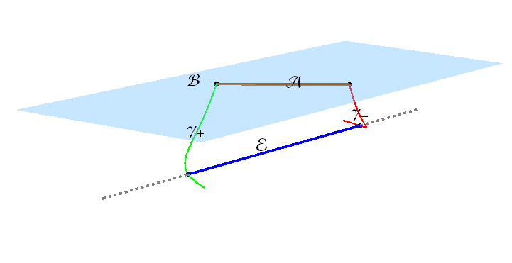
Figure 1: The blue solid line is the $\mathcal{E}_{\mathcal{A}}$ which is regulated from the spacelike geodesic $\mathcal{E}$. The red and green lines are the null geodesics $\gamma_{\pm}$ that connect the endpoints of $\mathcal{E}_{\mathcal{A}}$ and $\mathcal{A}$.

The above results also imply that the prescription to regulate the $\mathcal{E}$ via the UV/IR cutoff relations is different from the RT formula. Instead of being cut off at an infinitely large radius, the IR cutoff of the curve $\mathcal{E}$ in these cases are at finite radius and in some way controlled by the null geodesics $\gamma_{\pm}$ emanating from $\partial\mathcal{A}$. In this paper we try to understand this new geometric picture following the LM prescription Lewkowycz:2013nqa . We focus on the case of AdS₃/WCFT correspondence. In this holography the gravity side is AdS₃ with the Compere-Song-Strominger (CSS) Compere:2013bya boundary conditions while the field theory side is a WCFT. We study the replica story both on the boundary and in the bulk and try to understand the role of the null geodesics $\gamma_{\pm}$ in the replica story.

We will not re-derive the two main results of Lewkowycz:2013nqa ; Dong:2016hjy listed above and admit they are true in general holographies. However, to intrinsically determine the geometric picture for holographic entanglement entropy we need to solve the remaining two problems:

• how to determine the bulk extremal surface $\mathcal{E}$ in the bulk that matches $\mathcal{A}$ if we do not require $\mathcal{E}$ to be anchored on $\partial\mathcal{A}$?

• how to regulate $\mathcal{E}$ in the bulk accordingly when we regulate $\mathcal{A}$ on the boundary?

The above two problems are the main tasks of this paper. To solve the first problem, we need to explicitly study the causal structure of the boundary field theory and find its match in the bulk. In this paper we will not discuss topological ambiguities to determine $\mathcal{E}$. To solve the second problem, we use the prescription of Wen:2018whg to study the fine structure in holographic entanglement. More explicitly we use a new geometric quantity named the modular plane, to slice the entanglement wedge. Under this construction we get a fine correspondence between the points on $\mathcal{A}$ and the points on $\mathcal{E}$. We will show that the point where we cut $\mathcal{A}$ off and the point where we cut $\mathcal{E}$ off are just related by this fine correspondence.

The structure of this paper is in the following. In section 2 we present some interesting observations from the Rindler method which partially inspire the intrinsic prescription we will propose. Then we focus on the case of AdS₃/warped CFT correspondence. In section 3 we apply the Rindler method to this case. In section 4 we will explicitly study the bulk and boundary modular flows and define the modular planes. In section 5, we calculate the generalized gravitational entropy for AdS₃ with CSS boundary conditions with the help of modular planes. The goal of this section is to understand how do the null geodesics (or modular planes) relate the boundary and bulk cutoffs. Based on the above construction, in section 6 we propose an intrinsic prescription of calculate the generalized gravitational entropy for spacetimes with non-Lorentzian duals. At last, we apply our prescription to 3-dimensional flat holography in section 7. In appendix A, we classify the spacelike geodesics in AdS₃. The appendix B and C are written for special readers, who are interested in the saddle point condition for $\mathcal{E}_{\mathcal{A}}$ and the entanglement contour for WCFT.

2 New observations from the Rindler method

2.1 A brief introduction to Rindler method

In the field theory, the key step of the Rindler method is to construct a Rindler transformation, a symmetry transformation which maps the calculation of entanglement entropy to thermal entropy. The general strategy to construct Rindler transformations and their bulk extensions by using the symmetries of the field theory and holographic dictionary, is summarized in the section 2 of Jiang:2017ecm . Here we just give the main points of the Rindler method.

Consider a QFT on manifold $\mathcal{B}$ with the symmetry group $G$. The global symmetries, whose generators are denoted by ${h_{j}}$, form a subset of $G$. The Rindler transformations $R$, which map a subregion $\mathcal{D}$ of $\mathcal{B}$ to a Rindler space $\tilde{\mathcal{B}}$ with infinitely far away boundary, can be constructed by imposing the following requirements:

1. The transformations $R:~{}\tilde{x}^{i}=f(x^{i})$ should be a symmetry transformation of the QFT.

2. The vectors $\partial_{\tilde{x}^{i}}$ in the Rindler space should be a linear combination of the global generators in the original space

   $$\partial_{\tilde{x}^{i}}=\sum_{j}b_{ij}h_{j}\,,$$ (2.3)

   where $b_{ij}$ are arbitrary constants.

The first requirement will give constraints on the coefficients $b_{ij}$. The remaining independent coefficients will control the size, position of $\mathcal{D}$ and the thermal circle of $\tilde{\mathcal{B}}$. Note that the shape of $\mathcal{D}$ is determined by the symmetries and independent of the choice of $b_{ij}$. The Rindler transformation $R$ will be invariant under some imaginary identification of the Rindler coordinates $\tilde{x}^{i}\sim\tilde{x}^{i}+i{\tilde{\beta}}^{i}$. This identification can be referred to as a “thermal” identification in $\tilde{\mathcal{B}}$.

Our strategy to construct Rindler transformations only involves the global generators, thus has a natural extension in the bulk. According to the holographic dictionary, the global generators $h_{i}$ of the asymptotic symmetry group are dual to the isometries of the bulk sapcetime. Then by replacing the $h_{i}$ generators with the generators of the bulk isometries and requiring the Rindler bulk space to satisfy the same boundary conditions, we can get the Rindler transformations in the bulk. The bulk extension of $\tilde{\mathcal{B}}$ (or the Rindler bulk) should have a horizon whose Bekenstein-Hawking entropy gives the thermal entropy of the field theory on $\tilde{\mathcal{B}}$. Using the inverse bulk Rindler transformations we can map this horizon back to the bulk extension of the original field theory on $\mathcal{B}$. The image of this mapping will give the corresponding geometric quantity $\mathcal{E}$. One can consult Song:2016gtd ; Jiang:2017ecm for explicit examples of the Rindler method.

2.2 New observations from the Rindler method

In Jiang:2017ecm , with the inverse bulk Rindler transformations, the authors made several interesting observations.

• Observation 1: the horizon of the Rindler bulk space is mapped to two codimension one null hypersurfaces $\mathcal{N}_{\pm}$ in the original bulk space. The curve $\mathcal{E}$ that related to entanglement entropy is the curve where $\mathcal{N}_{-}$ intersect with $\mathcal{N}_{+}$,

  $$\mathcal{E}=\mathcal{N}_{-}\cap\mathcal{N}_{+}\,.$$ (2.4)

• Observation 2: the Hamiltonian in the Rindler bulk space and boundary $\tilde{\mathcal{B}}$ will be mapped to the modular Hamiltonian in the original bulk and boundary respectively. A modular flow $k_{t}$ ($k_{t}^{bulk}$) is generated by the modular Hamiltonian. Then the curve $\mathcal{E}$ is determined by

  $$k_{t}^{bulk}(\mathcal{E})=0\,,$$ (2.5)

  which means $\mathcal{E}$ is the fixed points of the modular flow.

• Observation 3: the two null hypersurfaces $\mathcal{N}_{\pm}$ are normal to $\mathcal{E}$. Furthermore their intersection with the boundary $\mathcal{B}$ gives a decomposition on $\mathcal{B}$, which is consistent with the causal structure of the dual field theory.

Although these observations are made in 3d flat holography, the logic behind them should work for general holographies. The first observation is just a mapping from the Rindler bulk to the original spacetime and follows the logic of Rindler method. The second way is equivalent to the statement that $\mathcal{E}$ is the fixed points of the bulk replica symmetry which is a key statement of the LM prescription Lewkowycz:2013nqa . In the third observation, the requirement that the bulk and boundary causal structure should be consistent is obviously a requirement of holography. Later we will explicitly show that the above observations are also true in the context of AdS₃/WCFT.

Note that, the ways (2.4) and (2.5) to determine $\mathcal{E}$ are not intrinsic and rely on the explicit information of the Rindler transformations and locally defined modular Hamiltonian, which may not even exist. However the third observation implies that, on the other way around, $\mathcal{E}$ can be determined by the requirement that, the bulk causal decomposition by the normal null hypersurfaces $\mathcal{N}_{\pm}$ of $\mathcal{E}$ should reproduce the causal structure of the boundary field theory associated to $\mathcal{A}$, i.e.

$$\mathcal{E}:~{}~{}\mathcal{N}_{\pm}\cap\mathcal{B}\supset\partial\mathcal{D}_{\mathcal{A}}$$ (2.6)

This prescription to determine $\mathcal{E}$ is intrinsic and can be applied for general spacetimes, thus finishes our first task.

The above construction remind us of the construction of the light-sheet by Bousso Bousso:2002ju . In Hubeny:2007xt , using the light-sheets the authors propose a prescription to construct the covariant geometric picture for entanglement entropy in the context of AdS/CFT. They require the light-sheet associated to $\mathcal{E}$ should intersect with the boundary on the boundary light-sheet associated to $\partial\mathcal{A}$. This is equivalent to our requirement of the consistency between the bulk and boundary causal structures (2.6).

3 Rindler method applied on the AdS₃/WCFT correspondence

3.1 AdS₃ with CSS boundary conditions

Let us give a quick review on the AdS₃/WCFT correspondence. In the Fefferman-Graham gauge, solutions to 3-dimensional Einstein gravity with a negative cosmological are in the following,

$${ds^{2}\over\ell^{2}}={d\eta^{2}\over\eta^{2}}+\eta^{2}\Big{(}g^{(0)}_{ab}+{1\over\eta^{2}}g^{(2)}_{ab}+{1\over\eta^{4}}g^{(4)}_{ab}\Big{)}dx^{a}dx^{b}\,,$$ (3.7)

where $\eta$ is the radial direction, and $x^{a},\,a=1,2$ parametrize the boundary. Under the Dirichlet boundary (Brown-Henneaux) conditions $\delta g_{ab}^{(0)}=0$, the asymptotic symmetry are generated by two copies of Virasoro algebra Brown:1986nw , which indicates the dual field theory is a CFT₂.

In Compere:2013bya , a Dirichlet-Neumann type of boundary conditions

$$\delta g^{(0)}_{\pm-}=0\,,\quad\partial_{-}g^{(0)}_{++}=0\,,\quad\delta g^{(2)}_{--}=0\,,$$ (3.8)

is considered for AdS₃ in Einstein gravity, which we refer as the CSS boundary conditions. Under the CSS boundary conditions the metric on the boundary is no longer fixed and is allowed to fluctuate. Without a fixed background metric the usual way to determine the causal structure of the boundary field theory with null geodesics (or hypersurfaces) associated to $\partial\mathcal{A}$ is meaningless. In these cases, one can still define the causal development $\mathcal{D}_{\mathcal{A}}$ as the subregion in $\mathcal{B}$, which is mapped to the whole Rindler space $\tilde{\mathcal{B}}$ under Rindler transformations (see section 2.1). This definition of causal development is more general, and will reduce to the definition using null lines when the boundary has a fixed background metric.

Consider a BTZ metric

$$ds^{2}=\ell^{2}\left(T_{u}^{2}du^{2}+2rdudv+T_{v}^{2}dv^{2}+\frac{dr^{2}}{4\left(r^{2}-T_{u}^{2}T_{v}^{2}\right)}\right)\,.$$ (3.9)

When we impose the CSS boundary conditions, the asymptotic symmetry group is featured by a Virasoro-Kac-Moody algebra Compere:2013bya ,

$$[\tilde{L}_{n},\tilde{L}_{m}]= (n-m)\tilde{L}_{n+m}+\frac{\tilde{c}}{12}(n^{3}-n)\delta_{n+m}\,,$$ (3.10)

$$[\tilde{L}_{n},\tilde{P}_{m}]= -m\tilde{P}_{m+n}+m\tilde{P}_{0}\delta_{n+m}\,,$$ (3.11)

$$[\tilde{P}_{n},\tilde{P}_{m}]= \frac{\tilde{k}}{2}n\delta_{m+n}\,,$$ (3.12)

with the central charge and Kac-Moody level given by

$$\tilde{c}= \frac{3\ell}{2G}\,,\qquad\tilde{k}=-\frac{\ell T_{v}^{2}}{G}\,.$$ (3.13)

Here we have set $T_{v}$ fixed to satisfy the boundary condition $\delta g^{(2)}_{--}=0$. Then $u$ is the direction that keeps the $SL(2,R)$ global symmetry. Although the local isometries in the bulk are still $SL(2,R)\times SL(2,R)$, only the $SL(2,R)\times U(1)$ part consists with the boundary conditions.

The above asymptotic symmetry analysis indicates that the dual field theory is a WCFT featured by the algebra (3.10). The WCFT has the following local symmetries Detournay:2012pc

$$u=f(u^{\prime})\,,\qquad v=v^{\prime}+g(u^{\prime})\,.$$ (3.14)

A Similar story of asymptotic symmetry analysis happens for warped AdS₃ Compere:2009zj , and the WAdS/WCFT correspondence Detournay:2012pc is conjectured.

The (warped) AdS₃/WCFT correspondence has passed several key tests by matching the thermal entropy Detournay:2012pc , entanglement entropy Castro:2015csg ; Song:2016gtd , correlation functions Song:2017czq and one-loop determinants Castro:2017hpx . See Compere:2013aya ; Hofman:2014loa ; Jensen:2017tnb for a few examples of WCFT models.

Note that the Kac-Moody level in (3.10) is charge dependent. This is different from the canonical warped CFT algebra Detournay:2012pc which has a constant Kac-Moody level. These two algebras can be related by a state dependent coordinate transformation. One can also obtain the canonical algebra using the state-dependent asymptotic Killing vectors Apolo:2018eky . The mapping between the entanglement entropies of the theories featured by these two algebras is explicitly discussed in Song:2016gtd . In this paper, by WCFT we mean the theory featured by the algebra (3.10), and will not do the further mapping to the canonical ones.

3.2 Rindler method for AdS₃ with CSS boundary conditions

The global symmetries of the asymptotic symmetry group of AdS₃ with CSS boundary conditions are $SL(2,R)\times U(1)$, which consist of the following generators

$$J_{-}=\partial_{u},\quad J_{0}=u\partial_{u}-r\partial_{r},\quad J_{+}=u^{2}\partial_{u}-\frac{1}{2r}\partial_{v}-2ru\partial_{r},\quad\bar{J}=\partial_{v}\,,$$ (3.15)

Now we consider the AdS₃ with $T_{u}=0,T_{v}=1$, and the AdS radius being $\ell=1$,

$$ds^{2}=2rdudv+(dv)^{2}+\frac{(dr)^{2}}{4r^{2}}\,.$$ (3.16)

On the boundary we choose the interval to be

$$\mathcal{A}:~{}~{}\{(-\frac{l_{u}}{2},-\frac{l_{v}}{2})\to(\frac{l_{u}}{2},\frac{l_{v}}{2})\}\,,$$ (3.17)

One can consult Song:2016gtd for the cases with general temperatures.

Following the strategy presented in section 2.1, we can construct the most general Rindler transformations (see appendix A in Song:2016gtd ). The coefficients $b_{ij}$ control the position, the size of $\mathcal{D}$ and the thermal circle of $\tilde{\mathcal{B}}$. Here for simplicity, we settle down the position of $\mathcal{D}$ and the thermal circle of $\tilde{\mathcal{B}}$, which do not affect the entanglement entropy. Then we get the Rindler transformations from the AdS₃ (3.16) to a Rindler $\widetilde{\text{AdS}_{3}}$ with $T_{\tilde{u}}=T_{\tilde{v}}=1$

$$ds^{2}=d\tilde{u}^{2}+2\tilde{r}d\tilde{u}d\tilde{v}+d\tilde{v}^{2}+\frac{d\tilde{r}^{2}}{4\left(\tilde{r}^{2}-1\right)}\,,$$ (3.18)

The Rindler transformations are given by

$$\tilde{u}= \frac{1}{4}\log\left(\frac{R_{-}^{2}-1}{R_{+}^{2}-1}\right)\,,$$ (3.19)

$$\tilde{v}= \frac{1}{4}\log\left(\frac{(R_{+}-1)(R_{-}+1)}{(R_{+}+1)(R_{-}-1)}\right)+v\,,$$ (3.20)

$$\tilde{r}= \frac{(R_{+}-1)(R_{-}-1)}{R_{+}+R_{-}}+1\,,$$ (3.21)

where

$$R_{\pm}=r(l_{u}\mp 2u)\,.$$ (3.22)

Asymptotically, we get

$$\tilde{u}=\text{Arctanh}\left(\frac{2u}{l_{u}}\right)\,,\qquad\tilde{v}=v\,,$$ (3.23)

which, as expected, is a warped conformal mapping (3.14). We see that the $(\tilde{u},\tilde{v})$ coordinates only cover a strip-like subregion

$$\mathcal{D}:~{}-\frac{l_{u}}{2}<u<\frac{l_{u}}{2}\,.$$ (3.24)

We define this strip $\mathcal{D}$ as the causal development of the interval $\mathcal{A}$ (see also Castro:2015csg ) in WCFT.

The bulk Rindler transformations (3.19) map the horizon of the Rindler $\widetilde{\text{AdS}_{3}}$ at $\tilde{r}=1$ to two null hypersurfaces $\mathcal{N}_{\pm}$,

$$\mathcal{N}_{+}:~{}~{}r=\frac{1}{l_{u}-2u},\qquad\mathcal{N}_{-}:~{}~{}r=\frac{1}{l_{u}+2u}.$$ (3.25)

We find $\mathcal{N}_{\pm}$ intersect at a curve in the bulk

$$\mathcal{E}=\mathcal{N}_{-}\cup\mathcal{N}_{+}:~{}~{}~{}~{}\left\{u=0\,,r=\frac{1}{l_{u}}\right\},$$ (3.26)

which is just the curve found in Song:2016gtd that related to the holographic entanglement entropy. This is exactly the observation 1 we made from Rindler method.

Also it is easy to see that, $\mathcal{N}_{\pm}$ intersect with the asymptotic boundary on $u=\pm\frac{l_{u}}{2}$, thus enclose a strip $-\frac{l_{u}}{2}<u<\frac{l_{u}}{2}$ on the boundary, which is just the strip region $\mathcal{D}$ (3.24). This confirms our observation 3 if $\mathcal{N}_{\pm}$ are normal to $\mathcal{E}$ (see section 4).

According to the logic of Rindler method, the thermal entropy for $\widetilde{\text{AdS}_{3}}$ gives the entanglement entropy of $\mathcal{A}$. Since the thermal entropy is infinite, we need to regulate the interval $\mathcal{A}$ by a cutoff $\epsilon_{u}$ along the $u$ direction, such that

$$\mathcal{A}_{reg}:~{}~{}\left\{(-\frac{l_{u}}{2}+\epsilon_{u},-\frac{l_{v}}{2})\to(\frac{l_{u}}{2}-\epsilon_{u},\frac{l_{v}}{2})\right\}\,.$$ (3.27)

As a consequence the extension of the horizon in Rindler $\widetilde{\text{AdS}_{3}}$ and the curve $\mathcal{E}$ in the original AdS₃ are also regulated. We find the regulated $\mathcal{E}$ is given by Song:2016gtd

$$\mathcal{E}_{reg}:~{}\left\{(u,v,r)|~{}u=0,~{}r=\frac{1}{l_{u}},~{}v=\ell\left(l_{v}+\log\frac{l_{u}}{\epsilon_{u}}\right)(\eta-\frac{1}{2}),~{}~{}~{}~{}\eta\in[0,1]\right\}\,.$$ (3.28)

We see that $\mathcal{E}$ is cut off in the bulk at a finite radius $r=\frac{1}{l_{u}}$, rather than the asymptotic boundary. The holographic entanglement entropy is then given by

$$S_{\text{EE}} =\frac{Length(\mathcal{E}_{reg})}{4G}=\frac{1}{4G}\left(l_{v}+\log\frac{l_{u}}{\epsilon_{u}}\right)\,.$$ (3.29)

Note that there is no need to introduce the cutoff $\epsilon_{v}$ along the $v$ direction since it can be taken to be zero without introducing extra divergence to the entanglement entropy.

Before going on, let us comment on the case of WAdS₃/WCFT. As was pointed out in Song:2016gtd , the Rindler method applied on warped AdS₃ is indeed the same as the above story on AdS₃, because the warping factor appears in neither the Rindler transformations nor the thermodynamic quantities. For simplicity we only focus on the case of AdS₃/WCFT.

4 Modular flows and modular planes

The Rindler method can also help us find the explicit formula for the modular flow. The generator of the normal Hamiltonian in Rindler space or Rindler bulk, which maps to the modular Hamiltonian in the original space, is the generator along the thermal circle, i.e. $k_{t}\equiv{\tilde{\beta}}^{i}\partial_{\tilde{x}^{i}}$. Since $\partial_{\tilde{x}^{i}}$ can be written as a linear combination of the global generators, $k_{t}$ should have the same property. Using the holography dictionary, we can easily get the bulk dual of $k_{t}$, which we call $k_{t}^{bulk}$. In order to map it to the original space, we need to solve the following differential equations

$$\partial_{u} =(\partial_{u}\tilde{u})\partial_{\tilde{u}}+(\partial_{u}\tilde{v})\partial_{\tilde{v}}+(\partial_{u}\tilde{r})\partial_{\tilde{r}}\,,$$ (4.30)

$$\partial_{v} =(\partial_{v}\tilde{u})\partial_{\tilde{u}}+(\partial_{v}\tilde{v})\partial_{\tilde{v}}+(\partial_{v}\tilde{r})\partial_{\tilde{r}}\,,$$ (4.31)

$$\partial_{r} =(\partial_{r}\tilde{u})\partial_{\tilde{u}}+(\partial_{r}\tilde{v})\partial_{\tilde{v}}+(\partial_{r}\tilde{r})\partial_{\tilde{r}}\,.$$ (4.32)

So we can get $\partial_{\tilde{u}},\partial_{\tilde{v}},\partial_{\tilde{r}}$, and furthermore $k_{t}^{bulk}$, in terms of $\partial_{u},\partial_{v},\partial_{r}$.

We plug (3.19) into (4.30). Solving the equations we get the bulk and boundary modular flow

$$k_{t}^{bulk} =-\tilde{\beta}_{\tilde{u}}\partial_{\tilde{u}}+\tilde{\beta}_{\tilde{v}}\partial_{\tilde{v}}=\pi\left(\partial_{\tilde{v}}-\partial_{\tilde{u}}\right)$$ (4.33)

$$=\frac{\pi\left(r^{-2}+4u^{2}-l_{u}^{2}\right)}{2l_{u}}\partial_{u}+\left(\pi-\frac{\pi}{l_{u}r}\right)\partial_{v}-\frac{4\pi ru}{l_{u}}\partial_{r}\,,$$ (4.34)

$$k_{t} =\frac{\pi\left(4u^{2}-l_{u}^{2}\right)}{2l_{u}}\partial_{u}+\pi\partial_{v}\,.$$ (4.35)

It is easy to check that the curve $\mathcal{E}$ (3.26) we find by Rindler method can also be determined by

$$k^{bulk}_{t}(\mathcal{E})=0\,.$$ (4.36)

This means $\mathcal{E}$ is the fixed points of $k^{bulk}_{t}$ (or the bulk replica symmetry) and confirms our observation 2. Obviously the endpoints of $\mathcal{A}$ are neither the fixed points of $k_{t}$ nor $k_{t}^{bulk}$. From the modular flow point of view, this means $\mathcal{E}$ should not be anchored on $\partial\mathcal{A}$, thus break the homology constraint.

We can get the explicit picture of the flow from (4.33) and (4.35). Solving the equation $(\frac{du(s)}{ds},\frac{dv(s)}{ds})=k_{t}$ we get the lines along modular flow on the boundary (see Fig.2),

$$\mathcal{L}_{v_{0}}:~{}~{}v=v_{0}-\text{arctanh}\frac{2u}{l_{u}}\,,$$ (4.37)

where $v_{0}$ is a integration constant that characterizes different modular flow lines. It is easy to see that $\mathcal{L}_{v_{0}}$ is anti-symmetric with respect to its middle point $(0,v_{0})$.

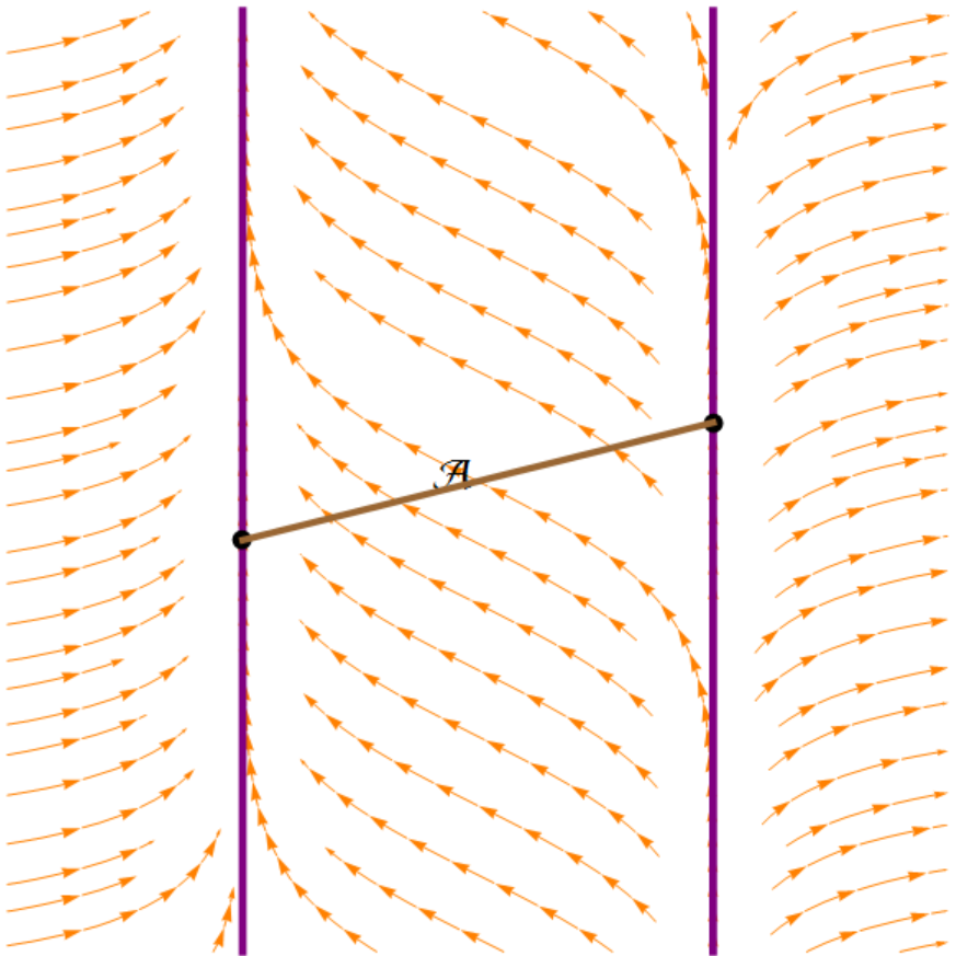
Figure 2: The orange lines with arrows depict the trajectory of the modular flow in WCFT. Note that the modular flow can never pass through $\partial\mathcal{D}$, which is depicted by the two purple lines.

Similarly, by solving the equation $(\frac{du(s)}{ds},\frac{dv(s)}{ds},\frac{dr(s)}{ds})=k_{t}^{bulk}$ we get the functions of the bulk modular flow lines $\bar{\mathcal{L}}_{\bar{v}_{0}}^{r_{0}}$ that are described by the following two branches of solutions

$$branch\,A :~{}~{}\Big{\{}\begin{array}[]{cc}&u(r)=-\frac{1}{2r}\sqrt{\frac{(r-r_{0})\left(l_{u}^{2}rr_{0}-1\right)}{r_{0}}}\,,\\ &v(r)=\bar{v}_{0}+\frac{1}{2}\log\left(\frac{1+l_{u}r+\sqrt{(r-r_{0})\left(l_{u}^{2}rr_{0}-1\right)/r_{0}}}{1+l_{u}r-\sqrt{(r-r_{0})\left(l_{u}^{2}rr_{0}-1\right)/r_{0}}}\right)\,,\\ \end{array}\quad-\frac{l_{u}}{2}<u\leq 0\,,$$ (4.40)

$$branch\,B :~{}~{}\Big{\{}\begin{array}[]{cc}&u(r)=\frac{1}{2r}\sqrt{\frac{(r-r_{0})\left(l_{u}^{2}rr_{0}-1\right)}{r_{0}}}\,,\\ &v(r)=\bar{v}_{0}-\frac{1}{2}\log\left(\frac{1+l_{u}r+\sqrt{(r-r_{0})\left(l_{u}^{2}rr_{0}-1\right)/r_{0}}}{1+l_{u}r-\sqrt{(r-r_{0})\left(l_{u}^{2}rr_{0}-1\right)/r_{0}}}\right)\,,\\ \end{array}\quad~{}~{}0\leq u<\frac{l_{u}}{2}\,.$$ (4.43)

The constants $r_{0}$ and $\bar{v}_{0}$ are the integration constants characterizing different bulk modular flow lines. The A branch part and B branch part smoothly connected at the point $(u,v,r)=(0,\bar{v}_{0},r_{0})$, which is the turning point of $\bar{\mathcal{L}}_{\bar{v}_{0}}^{r_{0}}$.

With the explicit picture of bulk and boundary modular flows, following Wen:2018whg we then define the geometric quantity which we call the modular plane. When $r\to\infty$, all $\bar{\mathcal{L}}_{\bar{v}_{0}}^{r_{0}}$ will anchor on the two lines $u=\pm\frac{l_{u}}{2}$ (or $\partial\mathcal{D}$) at the boundary. However when we push the boundary into the bulk a little, the class of $\bar{\mathcal{L}}_{\bar{v}_{0}}^{r_{0}}$ with $\bar{v}_{0}=v_{0}$, will intersect with the boundary on $\mathcal{L}_{v_{0}}$. This class of bulk modular flow lines forms a codimension one surface in the bulk, which we call the modular plane $\mathcal{P}(v_{0})$. In other words,

• the modular plane $\mathcal{P}(v_{0})$ is the orbit of the boundary modular flow line $\mathcal{L}_{v_{0}}$ under the bulk modular flow.

The modular planes are in one-to-one correspondence with the boundary modular flow lines. See Fig.3 for an explicit diagram for a modular plane. Later we will show that the modular planes play a crucial role on how we regulate $\mathcal{E}$ in the bulk.

Another class of bulk modular flow lines are those with $r_{0}=\frac{1}{l_{u}}$. The turning points are just the fixed points of $k_{t}^{bulk}$ on $\mathcal{E}$. It is easy to check that these modular flow lines are null and normal to $\mathcal{E}$, thus form the two normal null hypersurfaces $\mathcal{N}_{\pm}$ (3.25) emanating from $\mathcal{E}$. We denote this class of bulk modular flow lines as $\bar{\mathcal{L}}_{\bar{v}_{0}}$

$$\bar{\mathcal{L}}_{\bar{v}_{0}} :~{}~{}\Big{\{}\begin{array}[]{cc}&u=\frac{1}{2}\left(\frac{1}{r}-l_{u}\right),\qquad~{}~{}v=\bar{v}_{0}+\frac{1}{2}\log(l_{u}r)\,,\qquad branch~{}~{}A\,,\\ &u=-\frac{1}{2}\left(\frac{1}{r}-l_{u}\right),\qquad v=\bar{v}_{0}-\frac{1}{2}\log(l_{u}r)\,,\qquad branch~{}~{}B\,.\end{array}$$ (4.46)

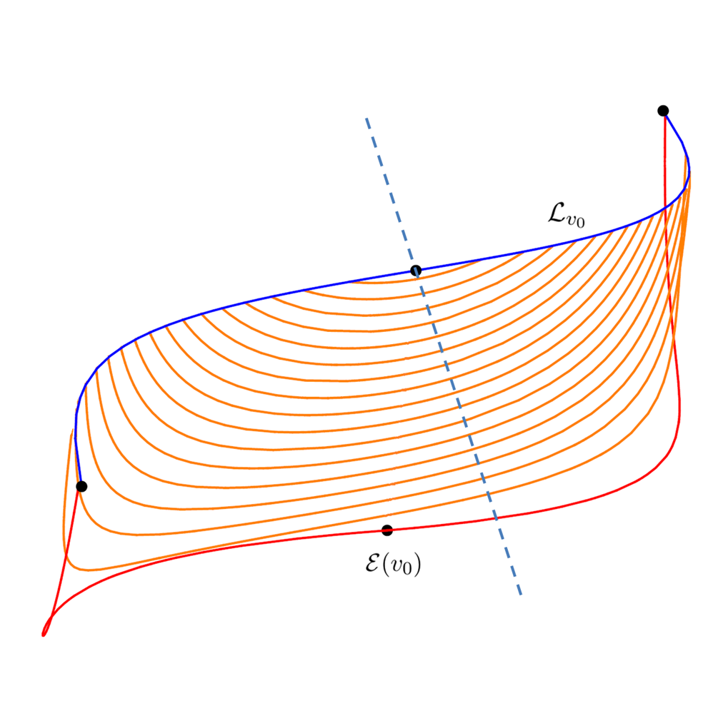
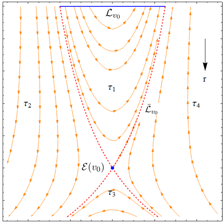
Figure 3: The left figure gives an explicit diagram for a modular plane $\mathcal{P}(v_{0})$. The blue line is $\mathcal{L}_{v_{0}}$ while the orange lines depict $\bar{\mathcal{L}}_{\bar{v}_{0}}^{r_{0}}$ with $\bar{v}_{0}=v_{0}\,,r>\frac{1}{l_{u}}$. The red line is $\bar{\mathcal{L}}_{v_{0}}$ with its turning point denoted as $\mathcal{E}(v_{0})$. The other two black points are where $\mathcal{L}_{v_{0}}$ intersect with the red line at $v=\pm\infty$. The right figure is just the projection of the left figure to a flat plane.

5 Generalized gravitational entropy for AdS₃ with CSS boundary conditions

In this section we try to understand how the LM prescription Lewkowycz:2013nqa ; Dong:2016hjy works in AdS₃ with the CSS boundary conditions. In the rest of this section, we will use the terminologies in Dong:2016hjy . For simplicity we will not repeat the Schwinger-Keldysh construction or time-folded path integral as in Dong:2016hjy , but calculate Tr$\rho_{\mathcal{A}}$ by performing the path integral over the whole spacetime. The generalization to the time-folded path integral can be obtained following the lines in Dong:2016hjy . We also try to extend the replica story of the boundary field theory into the bulk, and assume the replica symmetry is unbroken in the bulk. We will use (2.6) to determine the bulk extremal surface $\mathcal{E}$, and use the modular planes to relate the bulk and boundary cutoffs.

We will give the replica story for WCFT in subsection 5.1, then we construct the dual bulk replica story in subsection 5.2. Then in subsection 5.3 we follow the prescription in Wen:2018whg to study the fine structure of the bulk story using the modular planes. With the fine structure known, we will show the UV and IR cutoffs can be naturally related by the modular planes. At last, based on the fine structure analysis, we propose an intrinsic prescription of construct the geometric picture of entanglement entropy in subsection 5.4.

5.1 The replica story on the boundary

The field theory dual of AdS₃ (3.16) with CSS boundary conditions is a WCFT with the following thermal circle

$$(u,v)\sim(u,v-\pi i)\,.$$ (5.47)

The Rindler transformations decompose $\mathcal{B}$ into several regions with Rindler coordinates $(\tilde{u}_{i},\tilde{v}_{i})$. Similar to the strategy in Dong:2016hjy we can simultaneously refer to all these spacetime regions in question, by allowing the Rindler coordinates to be complex and assigning discrete imaginary parts to each region. The subscript $i$ denote different spacetime regions. Moving along the modular flow and jump from one region to another, we hop from one imaginary part to another. If eventually we jump back to our starting point, the imaginary parts we have gone through form a circle, which can be physically understood as the thermal circle measured by the Rindler observer. Putting all the regions together, whose imaginary parts form the total thermal circle, we should recover a pure state.

We cut the WCFT open along $\mathcal{A}$ then glue all the copies cyclically. We also need to know how the thermal circle changes under this cyclical gluing. The key to understand this is the assignment of the imaginary parts to all the spacetime regions. Since WCFT is not a relativistic field theory, its causal structure is quite abnormal compared with the relativistic ones, hence deserves discussion in detail.

For convenience, here we re-write the boundary Rindler transformation (3.23)

$$\tanh\left(\tilde{u}\right)=\frac{2u}{l_{u}}\,,\qquad\tanh\left(\tilde{v}\right)=\tanh v\,.$$ (5.48)

We write the second equation in such a way that the thermal circles in both of the original and Rindler space are exhibited in the coordinate transformation, i.e. (5.47) and

$$(\tilde{u},\tilde{v})\sim(\tilde{u}+\pi i,\tilde{v}-\pi i)\,.$$ (5.49)

Then it is convenient to confine

$$0\leq\text{Im}(\tilde{u})\leq i\pi\,,\qquad-i\pi\leq\text{Im}(\tilde{v})\leq 0\,.$$ (5.50)

Since the Rindler transformations divide the original spacetime $\mathcal{B}$ into three spacetime regions, we require the assignment of imaginary parts should consist with the Rindler transformations. In other words the Rindler transformations should map the Rindler space $(\tilde{u}_{i},\tilde{v}_{i})$ with different imaginary parts to different spacetime regions on $\mathcal{B}$. Furthermore we require the imaginary part of each region should be unique under the confinement (5.50) and different from the other regions.

Note that, the assignment is not uniquely determined by the above requirements. For example, for the strip region we can chose either the assignment $\text{Im}[(\tilde{u},\tilde{v})]=(0,0)$ or $\text{Im}[(\tilde{u},\tilde{v})]=(0,-i\pi)$. Both of the choices consist with the Rindler transformations. However all the choices satisfying our requirements can be related by a rotation or reversion of the thermal circle, thus do not change the physical story. Here we choose the following assignment for the three regions on $\mathcal{B}$

$$\text{Im}[(\tilde{u},\tilde{v})]=\Big{\{}\begin{array}[]{cc}~{}(0,0)\,,&\frac{l_{u}}{2}<u<\frac{l_{u}}{2}\,,\\ ~{}(\frac{\pi i}{2},0)\,,&u<-\frac{l_{u}}{2}\,,\\ (\frac{\pi i}{2},-\pi i)\,,&u>\frac{l_{u}}{2}\,.\end{array}$$ (5.54)

According to uniqueness requirement for the imaginary parts, there is no place on $\mathcal{B}$ for the assignment $\text{Im}[(\tilde{u},\tilde{v})]=(0,-\pi i)$. This can be understood in the following way. The state on $\mathcal{B}$ is already mixed, which indicates the complete thermal circle involves a region outside $\mathcal{B}$ that purifies $\mathcal{B}$. We denote this region as $\mathcal{B}^{c}$ and consider $\mathcal{B}\cup\mathcal{B}^{c}$ as the spacetime that recovers the pure state. So the proper assignment should be

$$\mathcal{B}^{c}:~{}~{}~{}~{}\text{Im}[(\tilde{u},\tilde{v})]=(0,-\pi i)\,.$$ (5.55)

We will see that the above assignment is quite natural in the gravity side story.

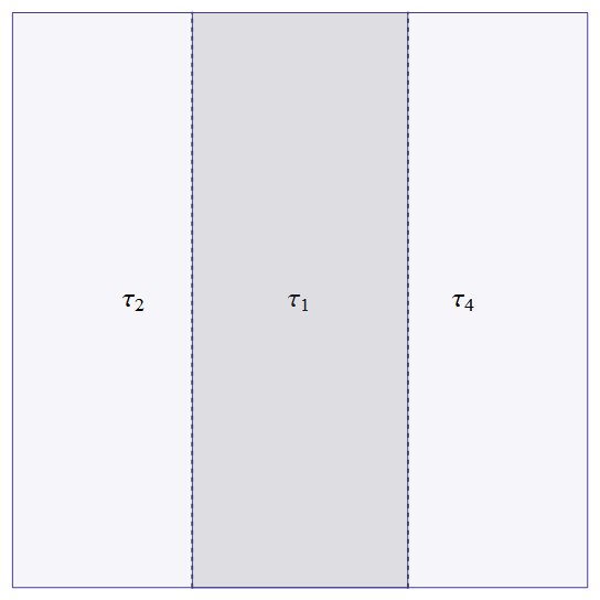
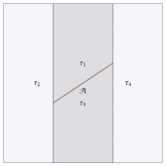
Figure 4: The causal decomposition for the WCFT, and the assignment of the imaginary parts for each region.

It will be more convenient to introduce the “Rindler time” $\tau=\tilde{u}-\tilde{v}$ such that

$$\tau_{m}=\tau+(m-1)\frac{\pi}{2}i\,.$$ (5.56)

The thermal circle becomes $\tau\sim\tau+2\pi i$ and the three regions on $\mathcal{B}$ can be denoted by $\tau_{1},\tau_{2}$ and $\tau_{4}$ (see the left figure in Fig.4), while the $\mathcal{B}^{c}$ can be denoted as $\tau_{3}$. For each time we cross the “horizon”, we add a $\frac{\pi}{2}i$ to $\tau$. We cut $\mathcal{A}$ open into $\mathcal{A}_{+}$ and $\mathcal{A}_{-}$ then the strip region is further divided into $\tau_{1},\tau_{5}$ (see the right figure in Fig.4).

Then we construct the replica story on the field theory side. We consider n copies of $\mathcal{B}$ and glue them cyclically

$$\phi_{I}(\mathcal{A}_{-})=\phi_{(I+1)}(\mathcal{A}_{+})\,,\qquad\phi_{n}(\mathcal{A}_{-})=\phi_{1}(\mathcal{A}_{+})\,,\qquad I=1,\cdots,n-1\,.$$ (5.57)

to calculate Tr($\rho_{\mathcal{A}}^{n}$). After the gluing we get a $n$-sheet manifold $\mathcal{B}_{n}$ with replica symmetry, where we perform the path integral. For $n=1$, the $\tau_{5}$ region is glued back to the $\tau_{1}$ region at $\mathcal{A}$, thus the thermal circle on $\mathcal{B}$ is $\tau\sim\tau+2\pi i$. Similarly we find the thermal circle on $\mathcal{B}_{n}$ becomes $\tau\sim\tau+2\pi ni$.

The fixed point of the thermal circle (or the replica symmetry) is where the thermal circle shrinks. More explicitly it should be the joint point of all the spacetime regions. However, unlike the case of CFT₂ (or other relativistic theories), there is no such point in WCFT. This is not surprising because $\mathcal{B}^{c}$ is outside $\mathcal{B}$ and $k_{t}$ (4.35) is nonvanishing everywhere on $\mathcal{B}$. In other words we have the replica symmetry, but there is no fixed point for this symmetry on $\mathcal{B}_{n}$.

5.2 The replica story in the bulk

In this subsection we try to construct the bulk extension of the boundary replica story. As in Lewkowycz:2013nqa ; Dong:2016hjy , we need to make the basic assumptions to extend the boundary replica story into the bulk. We assume the AdS₃/WCFT correspondence between the bulk and boundary theories and also we assume the replica symmetry can be extended into the bulk. According to Lewkowycz:2013nqa the curve $\mathcal{E}$ that is fixed under the bulk replica symmetry is extremal. For a given boundary subregion $\mathcal{A}$ and its causal development $\mathcal{D}_{\mathcal{A}}$, we determine the corresponding $\mathcal{E}$ by requiring that $\mathcal{E}$ and its null normal hypersurfaces $\mathcal{N}_{\pm}$ should satisfy (2.6). The $\mathcal{N}_{\pm}$ decompose the bulk into four regions denoted by $\tau_{m}$. Here $\tau_{m}$ parametrizes the bulk modular flows in each region.

Following the above strategy we search the geodesics in the bulk (for details see appendix A) and find that the geodesic satisfying (2.6) exists and is just the curve $\mathcal{E}$ (3.26) we found by Rindler method. This is not surprising since the $\mathcal{N}_{\pm}$ (3.25) are formed by the normal null geodesics associated to $\mathcal{E}$ and intersect with the boundary at $\partial\mathcal{D}_{\mathcal{A}}:~{}u=\pm\frac{l_{u}}{2}$. The bulk subregion enclosed by $\mathcal{B}$ and $\mathcal{N}_{\pm}$ is the analogue of the entanglement wedge $\mathcal{W}_{\mathcal{A}}$.

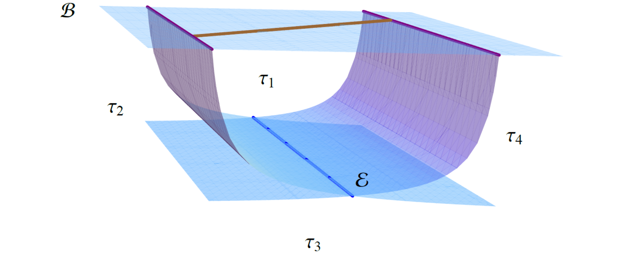
Figure 5: This figure shows the causal decomposition of the bulk $\mathcal{M}$ and the boundary $\mathcal{B}$. The two surfaces that intersect at $\mathcal{E}$ are $\mathcal{N}_{\pm}$ and the brown line is the boundary interval $\mathcal{A}$.

Now we try to construct the bulk replica story. We allow $\tau_{m}$ to be complex and refer to all the bulk regions in question by defining $\tau_{m}=\tau+\frac{(m-1)}{2}i\pi$. The assignment of the imaginary parts are explicitly shown in Fig.5. Note that the $\tau_{3}$ region in the bulk does not overlap with the boundary $\mathcal{B}$, thus confirms our statement that there is no $\tau_{3}$ region on $\mathcal{B}$. We expect the boundary branched cover structure inherent in the replica construction to be inherited by the holographic map in the bulk. The bulk geometry should be a replicated geometry glued cyclically from $n$ copies of the bulk spacetime.

Before we go ahead, we briefly review the bulk replica story in AdS/CFT Dong:2016hjy . In this case the RT surface $\mathcal{E}$ is anchored on $\partial\mathcal{A}$. We denote the spacelike codimension one surface enclosed by $\mathcal{E}$ and $\mathcal{A}$ as $\mathcal{R}_{\mathcal{A}}$, which satisfies $\partial\mathcal{R}_{\mathcal{A}}=\mathcal{A}\cup\mathcal{E}$. Firstly, for each copy of bulk $\mathcal{M}^{I}$, we cut them open along $\mathcal{R}^{I}_{\mathcal{A}}$ into $\mathcal{R}^{I}_{\mathcal{A}}{}_{+}$ and $\mathcal{R}^{I}_{\mathcal{A}}{}_{-}$. Then we get the replicated geometry by gluing the open cuts cyclically

$$\mathcal{R}^{I}_{\mathcal{A}}{}_{-}=\mathcal{R}^{(I+1)}_{\mathcal{A}}{}_{+}\,,\qquad\mathcal{R}^{n}_{\mathcal{A}}{}_{-}=\mathcal{R}^{1}_{\mathcal{A}}{}_{+}\,.$$ (5.58)

In the case of AdS/WCFT, in order to conduct the replica trick we also need to cut the bulk open along some codimension one surface, which we also denote as $\mathcal{R}_{\mathcal{A}}$. Since $\mathcal{E}$ is supposed to be fixed under the replica symmetry, we require $\mathcal{E}\subset\partial\mathcal{R}_{\mathcal{A}}$. On the boundary, we require $\mathcal{A}\subset\partial\mathcal{R}_{\mathcal{A}}$ to reproduce the boundary replica story. However, in this case $\mathcal{E}$ is not anchored on $\partial\mathcal{A}$, so $\partial\mathcal{R}_{\mathcal{A}}$ contains other parts. In addition, $\mathcal{R}_{\mathcal{A}}$ have two more boundaries $\gamma_{\pm}$ that connect the two endpoints $\partial\mathcal{A}_{\pm}$ of the boundary interval and the endpoints of $\mathcal{E}$ at $v=\pm\infty$. Later we will argue that $\gamma_{\pm}$ should be the null geodesics on $\mathcal{N}_{\pm}$. In summary we have

$$\partial\mathcal{R}_{\mathcal{A}}=\mathcal{A}\cup\mathcal{E}\cup\gamma_{+}\cup\gamma_{-}\,.$$ (5.59)

With $\partial\mathcal{R}_{\mathcal{A}}$ settled down, the surface $\mathcal{R}_{\mathcal{A}}$ has the freedom to vibrate as long as we keep $\mathcal{R}_{\mathcal{A}}$ spacelike everywhere except $\gamma_{\pm}$. Then we cut $\mathcal{R}_{\mathcal{A}}^{I}$ open to $\mathcal{R}_{\mathcal{A}+}^{I}$ and $\mathcal{R}_{\mathcal{A}-}^{I}$ in each copy of the bulk and then glue them cyclicly to the replicated geometry $\mathcal{M}_{n}$.

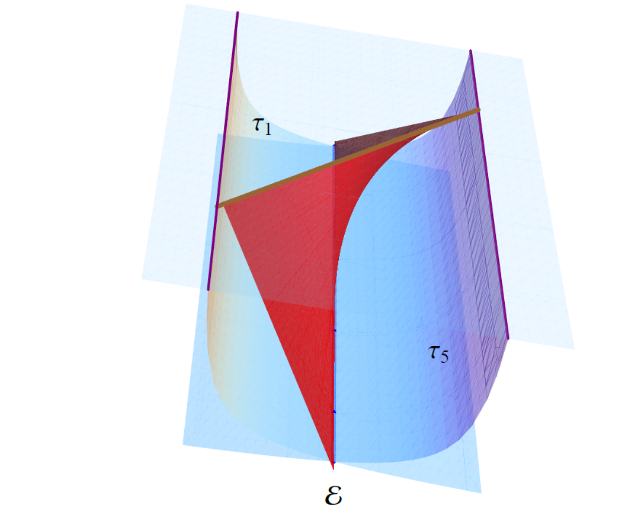
Figure 6: The red surface is the $\mathcal{R}_{\mathcal{A}}$ where we cut the bulk open.

Note that when we cut $\mathcal{R}_{\mathcal{A}}$ open we divide the $\tau_{1}$ region into two regions denoted by $\tau_{1}$ and $\tau_{5}$ (see Fig. 6). Starting from some point in the $\tau_{1}$ region, we move along a bulk modular flow line and cross the horizons $\mathcal{N}_{\pm}$ for four times to arrive at the $\tau_{5}$ region. Then we pass through $\mathcal{R}_{A}$ and enter the next copy of bulk spacetime. The cyclic gluing of $n$ copies of the bulk makes us pass through the horizons for 4$n$ times to get back to the starting point. This induces the thermal circle $\tau\sim\tau+2\pi ni$ in $\mathcal{M}_{n}$, which shrinks at $\mathcal{E}$. As expected the bulk replica story reproduces the boundary replica story.

5.3 Relating the UV and IR cutoffs with the modular planes (null geodesics)

Then we focus on our second task: how to regulate $\mathcal{E}$ when we regulate the boundary interval $\mathcal{A}$. In the case of AdS/CFT, the UV/IR relation Susskind:1998dq is used to regulate the holographic entanglement entropy in the RT formula. This prescription for regulation is also confirmed in Wen:2018whg by using the modular planes as a slicing of the entanglement wedge. The slicing gives a fine correspondence between the points on $\mathcal{A}$ and the points on the RT surface $\mathcal{E}$. Wen:2018whg shows that the points where we cut off $\mathcal{A}$ and $\mathcal{E}$ should be related by this fine correspondence.

In the case of AdS₃/WCFT, the curve $\mathcal{E}$ (3.26) can not be regulated following the RT formula. However, with the bulk and boundary modular flows clear, we can also define the modular planes as in Wen:2018whg and perform the fine structure analysis to determine the cutoff point in the bulk. As in the case of AdS₃/CFT₂ Wen:2018whg , we will show that the modular planes can regulate $\mathcal{E}$ correctly when we regulate $\mathcal{A}$.

The modular plane $\mathcal{P}(v_{0})$ is defined as the orbit of a boundary modular flow line $\mathcal{L}_{v_{0}}$ under the bulk modular flow, which is a codimension one surface in the bulk. Its construction in this case is discussed in details in section 4. The modular planes are in one-to-one correspondence with the boundary modular flow lines $\mathcal{L}_{v_{0}}$. By definition we have

$$\mathcal{P}(v_{0})\cap\mathcal{B}=\mathcal{L}_{v_{0}}\,.$$ (5.60)

As the boundary can be viewed as a slicing of modular flow lines $\mathcal{L}_{v_{0}}$, the entanglement wedge $\mathcal{W}_{\mathcal{A}}$ can also be viewed as a slicing of the modular planes $\mathcal{P}(v_{0})$. The normal null geodesics on $\mathcal{N}_{\pm}$ are also bulk modular flow lines, which indicates the modular planes will intersect with $\mathcal{N}_{\pm}$ on these normal null geodesics, i.e.

$$\mathcal{P}(v_{0})\cap\mathcal{N}_{\pm}=\bar{\mathcal{L}}_{v_{0}}\,.$$ (5.61)

It is easy to see that $\bar{\mathcal{L}}_{v_{0}}$ (or $\mathcal{P}(v_{0})$) intersect with $\mathcal{E}$ (3.26) at its turning point

$$\mathcal{P}(v_{0})\cap\mathcal{E}=\mathcal{E}(v_{0}):~{}(u,v,r)=(0,v_{0},\frac{1}{l_{u}})\,.$$ (5.62)

Also each modular plane will intersect with $\mathcal{R}_{\mathcal{A}}$ on a line

$$\mathcal{R}_{\mathcal{A}}(v_{0})=\mathcal{P}(v_{0})\cap\mathcal{R}_{\mathcal{A}}\,.$$ (5.63)

See Fig.3 for a typical modular plane.

Translation along a bulk modular flow line is a translation of the real part of $\tau_{m}$ while keeping the imaginary part fixed. When we apply the replica trick, the bulk and boundary are cyclically glued, the orbit of the modular flow changes, as well as the distribution of the imaginary part Im[$\tau$]. Let us focus on the cyclic gluing of a single point $\mathcal{A}(v^{\prime}_{0})$ and see how it changes the modular flow picture both in the bulk and boundary. Here $v^{\prime}_{0}$ denote the $v$ coordinate of the point $\mathcal{A}(v^{\prime}_{0})$. We denote the boundary modular flow line that passes this point as $\mathcal{L}_{v_{0}}$ given by (4.37). On the boundary, $\mathcal{L}_{v_{0}}$ will enter the next copy of $\mathcal{B}$ when it passes through $\mathcal{A}(v^{\prime}_{0})$. By definition all the bulk modular flow lines that emanating from $\mathcal{L}_{v_{0}}$ will return back to $\mathcal{L}_{v_{0}}$. As $\mathcal{L}_{v_{0}}$ enters the next copy of $\mathcal{B}$, the bulk modular flow emanating from $\mathcal{L}_{v_{0}}$ also need to enter the next copy of bulk to get back to the same $\mathcal{L}_{v_{0}}$. Then the natural bulk extension of the cyclic gluing of the point $\mathcal{A}(v^{\prime}_{0})$ is the cyclic gluing of the modular plane $\mathcal{P}(v_{0})$ on $\mathcal{R}_{\mathcal{A}}(v_{0})$, i.e.

$$\mathcal{R}_{\mathcal{A-}}^{I}(v_{0}) =\mathcal{R}_{\mathcal{A+}}^{I+1}(v_{0})\,,\qquad\mathcal{R}_{\mathcal{A-}}^{n}(v_{0})=\mathcal{R}_{\mathcal{A+}}^{1}(v_{0})\,.$$ (5.64)

We denote the cyclically glued modular plane as $\mathcal{P}_{n}(v_{0})$. Following the modular flows we can keep track of the imaginary part of $\tau$ everywhere on $\mathcal{P}_{n}(v_{0})$ and find the thermal circle on $\mathcal{P}_{n}(v_{0})$ becomes $\tau\sim\tau+2\pi ni$. Accordingly the induced metric near the fixed point $\mathcal{E}(v_{0})$ on $\mathcal{P}_{n}(v_{0})$ becomes

$$ds^{2}=n^{2}d\rho^{2}-\rho^{2}d\tau^{2}+\cdots,$$ (5.65)

where $\rho$ denotes the distance from $\mathcal{E}(v_{0})$, and the dots means the higher order terms. See Fig.7 for the replica story on the modular plane with $n=2$. The whole bulk replica story can be considered as a slicing of the replica stories on all the modular planes.

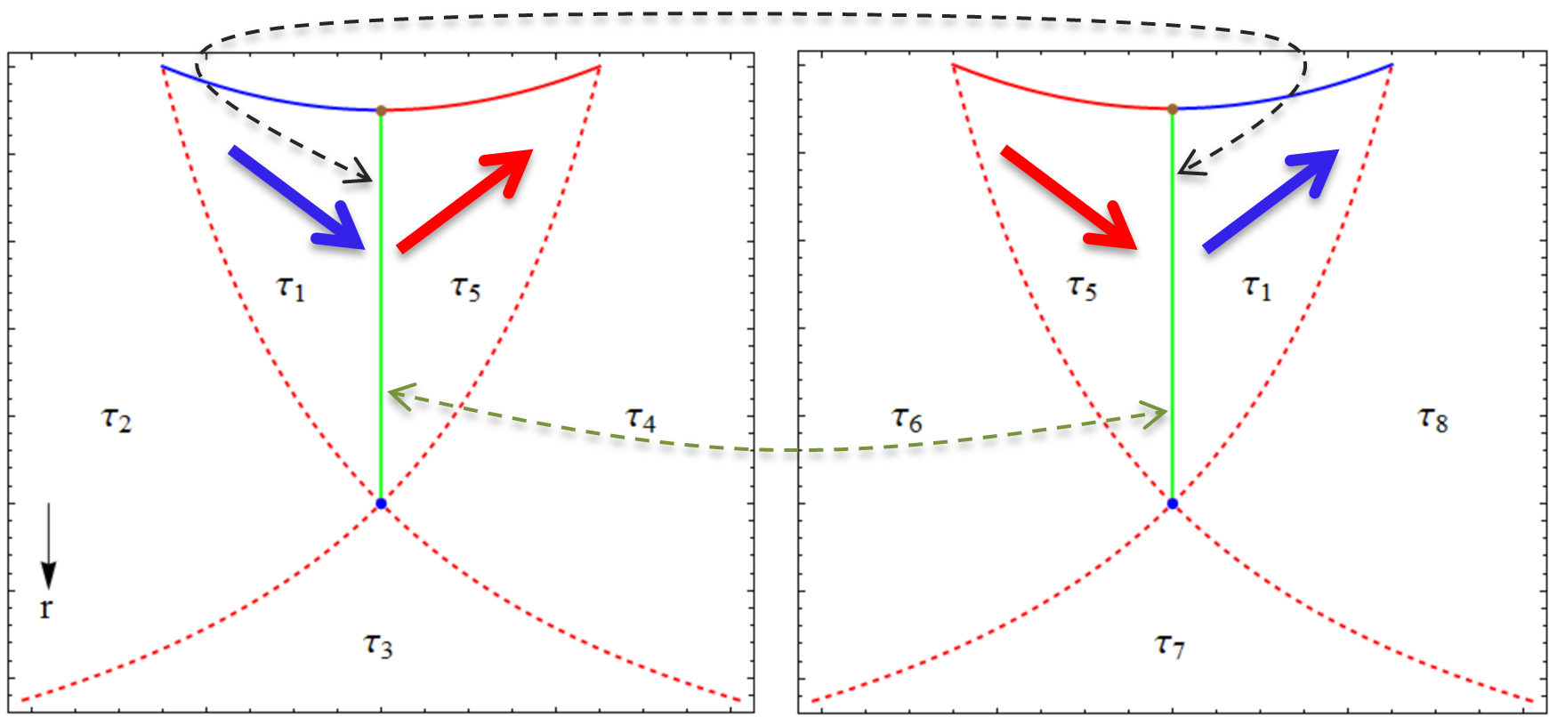
Figure 7: This figure is taken from Wen:2018whg and shows the replica story for a cyclically glued modular plane $\mathcal{P}_{n}(v_{0})$ with $n=2$. In the first copy the boundary modular flow line $\mathcal{L}_{v_{0}}$ parametrized by $\tau_{1}$ (blue line) passes through $\mathcal{A}(v_{0}^{\prime})$ and get into the next copy. The bulk flow (blue arrow) should also go through $\mathcal{R}_{\mathcal{A}}(v_{0})$ (the green line) to the next copy then go back to $\mathcal{L}_{v_{0}}$. A similar story happens to the flow lines parametrized by $\tau_{5}$ (the red line and arrow). The dashed arrows shows the cyclic gluing on $\mathcal{R}_{\mathcal{A}}(v_{0})^{1,2}$.

In summary, the cyclic gluing of a point $\mathcal{A}(v^{\prime}_{0})$ on the boundary interval induces a replica story on $\mathcal{P}_{n}(v_{0})$. Following the calculations in Lewkowycz:2013nqa ; Dong:2016hjy , this turns on nonzero contribution to the entanglement entropy on the fixed point $\mathcal{E}(v_{0})$ where the modular plane intersect with $\mathcal{E}$. In other words, this gives an one-to-one correspondence between the points $\mathcal{A}(v^{\prime}_{0})$ on $\mathcal{A}$ and the points $\mathcal{E}(v_{0})$ on $\mathcal{E}$ (see the left figure of Fig.8). More explicitly, if we consider $\mathcal{A}$ to be a straight line

$$\mathcal{A}:~{}~{}u=\frac{l_{u}}{l_{v}}v\,,\qquad-\frac{l_{v}}{2}\leq v\leq\frac{l_{v}}{2}\,,$$ (5.66)

the two points that correspond to each other are related by

$$v^{\prime}_{0}+\text{arctanh}\frac{2v^{\prime}_{0}}{l_{v}}=v_{0}\,.$$ (5.67)

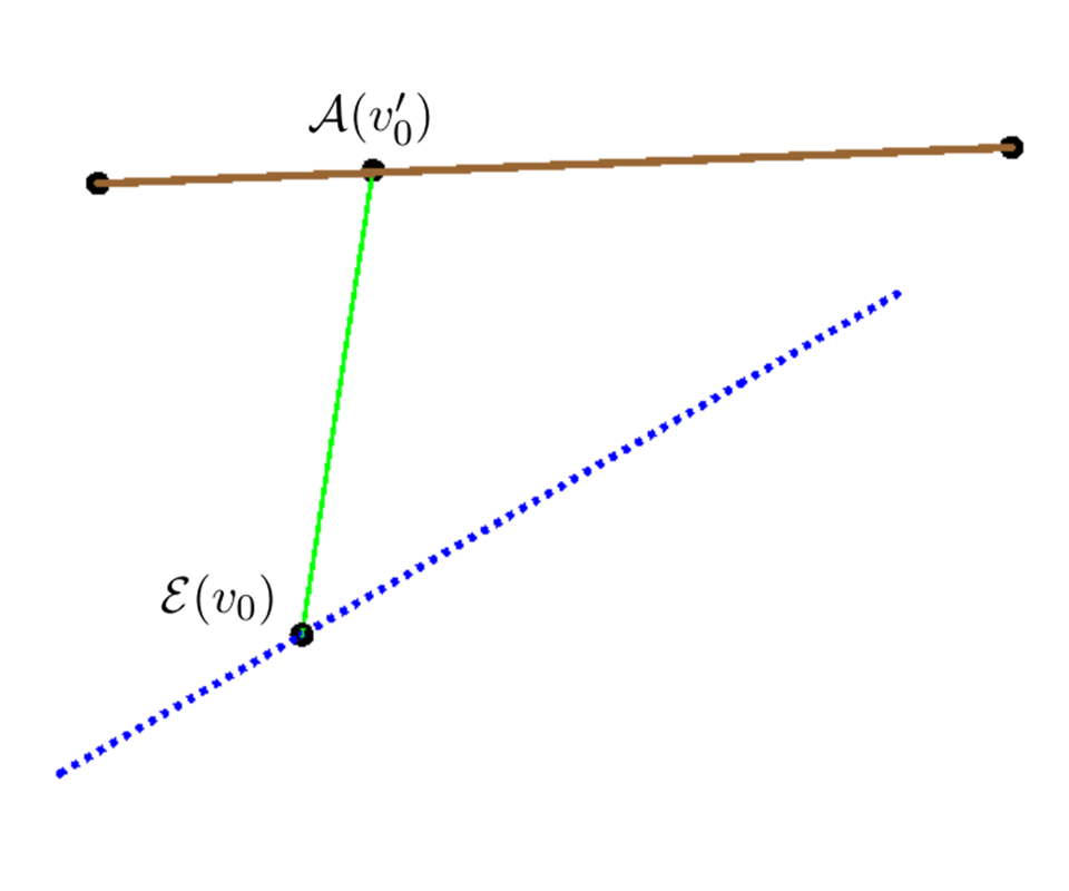
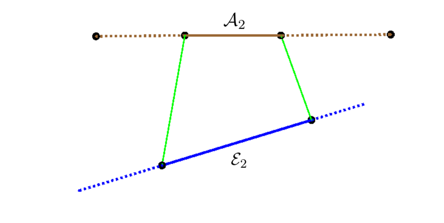
Figure 8: The right figure shows the correspondence between the point $\mathcal{A}(v^{\prime}_{0})$ on $\mathcal{A}$ and its partner $\mathcal{E}(v_{0})$ on $\mathcal{E}$ with $v_{0}$ and $v^{\prime}_{0}$ satisfying (5.67). Also they are the points where the modular plane $\mathcal{P}(v_{0})$ intersect with $\mathcal{A}$ and $\mathcal{E}$. The green line is $\mathcal{R}_{\mathcal{A}}(v_{0})$. The left figure shows, in the same sense, an arbitrary sub-interval $\mathcal{A}_{2}$ corresponds to a subinterval $\mathcal{E}_{2}$ on $\mathcal{E}$.

When $\mathcal{A}(v^{\prime}_{0})$ approaches $\partial_{\pm}\mathcal{A}$, i.e. $v^{\prime}_{0}=\pm\frac{l_{v}}{2}$, the partner points become $\mathcal{E}(v_{0}^{\pm})|_{v_{0}^{\pm}=\pm\infty}$. Note that the endpoints $\partial_{\pm}A$ also lie on the null hypersurfaces $\mathcal{N}_{\pm}$, they can be connected to their partners $\mathcal{E}(v_{0}^{\pm})$ by the two null geodesics $\gamma_{\pm}=\bar{\mathcal{L}}_{v_{0}^{\pm}}$. This indicates that all the lines that connect these two pair of points will contain timelike part except the two null lines $\gamma_{\pm}$. Since we do not expect time-like parts on the surface $\mathcal{R}_{\mathcal{A}}$, the only choice for $\mathcal{R}_{\mathcal{A}}(v_{0}^{\pm})$ are $\gamma_{\pm}$. This is how we determine $\partial\mathcal{R}_{\mathcal{A}}$ to be (5.59).

In the same sense, an arbitrary sub-interval $\mathcal{A}_{2}$ of $\mathcal{A}$ correspond to a sub-interval $\mathcal{E}_{2}$ on $\mathcal{E}$ (see the right figure of Fig.8). We denote the $v$ coordinate of the two endpoints of $\mathcal{A}_{2}$ as $v^{\prime}_{1}$ and $v^{\prime}_{2}$ and denote the $v$ coordinates of the two endpoints of $\mathcal{E}_{2}$ as $v_{1}$ and $v_{2}$. Similarly they should be related by (5.67). According to our prescription, the contribution from $\mathcal{E}_{2}$ to the total entanglement entropy $S_{\mathcal{A}}$ is turned on by the cyclic gluing of $\mathcal{A}_{2}$ on the boundary. Thus it is natural to propose that the length of $\mathcal{E}_{2}$ captures the contribution from the sub-interval $\mathcal{A}_{2}$ to $S_{\mathcal{A}}$. We denote this contribution as $s_{\mathcal{A}}(\mathcal{A}_{2})$ (see (B.133))

$$s_{\mathcal{A}}(\mathcal{A}_{2})=\frac{Length(\mathcal{E}_{2})}{4G}\,.$$ (5.68)

Let us go a step further and consider $\mathcal{A}_{2}=\mathcal{A}_{reg}$. It is natural to interpret the regulated entanglement entropy as the contribution from $\mathcal{A}_{reg}$. More explicitly we set

$$v^{\prime}_{1}=-\frac{l_{v}}{2}+\epsilon_{u}\frac{l_{v}}{l_{u}}\,,\qquad v^{\prime}_{2}=\frac{l_{v}}{2}-\epsilon_{u}\frac{l_{v}}{l_{u}}\,.$$ (5.69)

Then the end two points $\mathcal{E}(v_{1})$ and $\mathcal{E}(v_{2})$ of $\mathcal{E}_{2}=\mathcal{E}_{reg}$ should be the points where the geodesic $\mathcal{E}$ is cut off. Applying (5.67), we find

$$v_{1}=-\frac{1}{2}\left(l_{v}+\log\frac{l_{u}}{\epsilon_{u}}\right)+\mathcal{O}(\epsilon_{u})\,,\qquad v_{2}=\frac{1}{2}\left(l_{v}+\log\frac{l_{u}}{\epsilon_{u}}\right)+\mathcal{O}(\epsilon_{u})\,,$$ (5.70)

which are exactly the cutoff points we found by Rindler method. For an overall picture of our prescription, see Fig.9. The regulated entanglement entropy is then given by

$$S_{\mathcal{A}}=\frac{Length(\mathcal{E}_{reg})}{4G}=\frac{1}{4G}\left(l_{v}+\log\frac{l_{u}}{\epsilon_{u}}\right)\,.$$ (5.71)

As expected the result coincide with the result (3.29) we get by the Rindler method.

As was pointed out by Wen:2018whg , the fine correspondence between the points on $\mathcal{A}$ and the points on $\mathcal{E}$ defines an entanglement contour function that describes the distribution of the entanglement on $\mathcal{A}$. People who are interested in the entanglement contour should consult appendix B, where we calculate the contour function based on this fine correspondence (5.67), and furthermore we test the proposal Wen:2018whg for entanglement contour function for general theories.

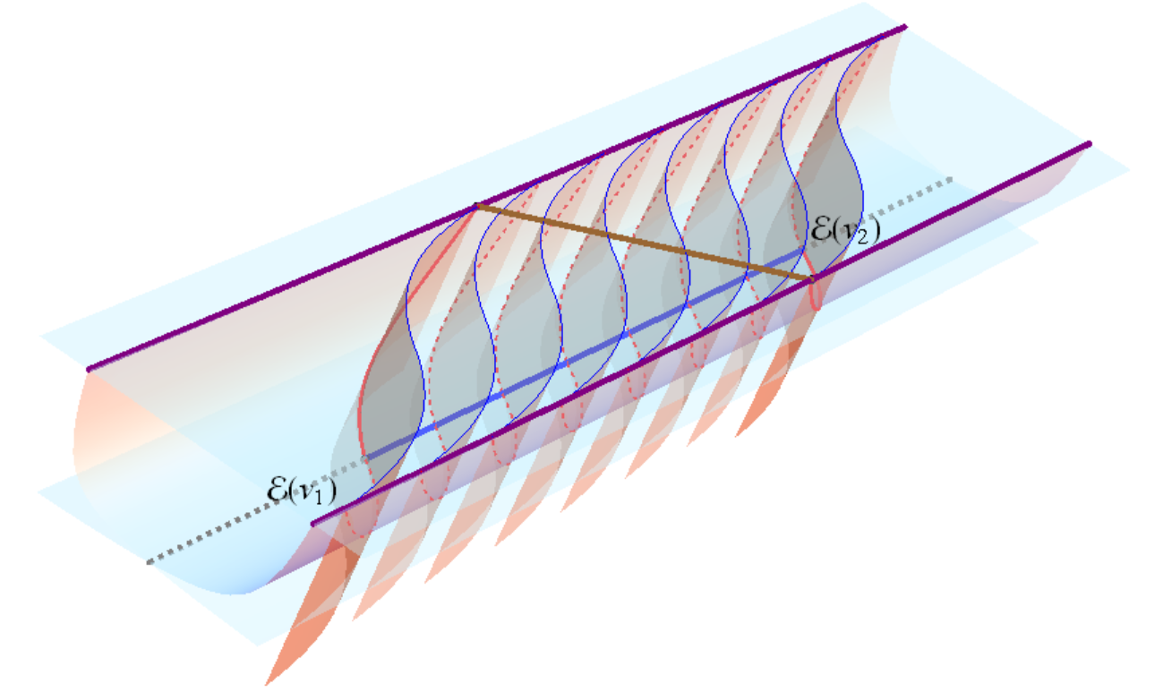
Figure 9: The entanglement wedge is shown as a slicing of the modular planes. We denote the thick blue line in the bulk as $\mathcal{E}_{reg}$. We only depicted the modular planes that go through $\mathcal{A}_{reg}$. The modular planes $\mathcal{P}(v_{1})$ and $\mathcal{P}(v_{2})$ intersect with $\mathcal{A}$ and $\mathcal{E}$ on the points where they are cut off.

5.4 The intrinsic construction of the geometric picture

The construction above is concrete but relies heavily on the explicit picture of the bulk and boundary modular flows, which is complicated to calculate and only exists for special cases. Then we come to the important question: is there a prescription to construct the geometric picture intrinsically without the construction of Rindler transformations and the information of the modular flows? Inspired by the above construction we try to propose such a prescription for the case we study.

The prescription also involves a cutoff at large radius $r_{I}$, which is related to the cutoff $\epsilon_{u}$ in the WCFT by

$$r_{I}=\frac{1}{\epsilon_{u}}\,.$$ (5.72)

In this case the radius cutoff is imposed on the two null geodesics $\gamma_{\pm}$ rather than the spacelike geodesic $\mathcal{E}$. However the way we impose this cutoff is a little tricky. The $\gamma_{\pm}$ emanating from the boundary endpoints $\partial_{\pm}\mathcal{A}$ at the real boundary will intersect with $\mathcal{E}$ at $v_{0}^{\pm}=\pm\infty$. So cutting off $\gamma_{\pm}$ at $r_{I}$ does not regulate the entanglement entropy.

The right way to do the regulation is in the following. We first need to push the WCFT to the cutoff boundary at $r=r_{I}$. During we push the boundary, we should keep $\partial_{\pm}\mathcal{A}$ on $\mathcal{N}_{\pm}$ thus adapt to the bulk causal decomposition. Furthermore we should keep the $v$ coordinate of $\partial_{\pm}\mathcal{A}$ fixed since there is no cutoff along the $v$ direction. Then the two null geodesics that emanating from the $\partial_{\pm}\mathcal{A}$ at $r=r_{I}$ will intersect with $\mathcal{E}$ on the right cutoff points (see Fig. 10).

Following the above prescription, the endpoints $\partial_{\pm}\mathcal{A}$ are pushed to the following positions

$$\partial_{\pm}\mathcal{A}:~{}~{}(\pm\frac{l_{u}}{2}\mp\frac{1}{2r_{I}},\pm\frac{l_{v}}{2},r_{I})\,.$$ (5.73)

Note that all the null geodesics $\bar{\mathcal{L}}_{\bar{v}_{0}}$ lie on $\mathcal{N}_{\pm}$ are given in (4.46) and $\bar{v}_{0}$ denotes the $v$ coordinate of the points where $\bar{\mathcal{L}}_{\bar{v}_{0}}$ intersect with $\mathcal{E}$. It is easy to find that the two null geodesics $\gamma_{\pm}$ emanating from $\partial_{\pm}\mathcal{A}$ (5.73) are just given by $\bar{\mathcal{L}}_{\bar{v}_{0}}$ with $\bar{v}_{0}=\pm(\frac{l_{v}}{2}+\frac{1}{2}\log(l_{u}r_{I}))$, i.e.

$$\gamma_{\pm}:~{}~{}u=\mp\frac{1}{2}\left(\frac{1}{r}-l_{u}\right),\qquad v=\pm\left(\frac{l_{v}}{2}+\frac{1}{2}\log(l_{u}r_{I})\right)\mp\frac{1}{2}\log(l_{u}r)\,.$$ (5.74)

When $r=\frac{1}{l_{u}}$ we get the end points of $\mathcal{E}_{reg}$. See Fig. 11 for an overall picture of our construction. The length of the regulated curve $\mathcal{E}_{reg}$ is just

$$Length(\mathcal{E}_{reg})=l_{v}+\log(l_{u}r_{I})\,,$$ (5.75)

which reproduces the result (5.71) with the UV/IR relation (5.72). In appendix C, we show that, similar to the flat case Jiang:2017ecm , the $\mathcal{E}_{reg}$ is the saddle among all the geodesics that connect $\gamma_{\pm}$ (5.74).

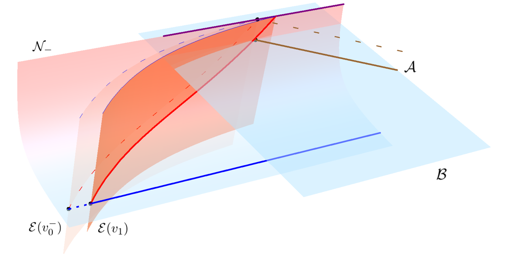
Figure 10: We assume $\mathcal{E}(v_{0}^{-})$, with $v_{0}^{-}=-\infty$, is the point that connected to $\partial_{-}\mathcal{A}$ on the real boundary through the null geodesics $\gamma_{-}$. When we push $\partial_{-}\mathcal{A}$ to the cutoff boundary along $\mathcal{N}_{-}$, the null geodesic $\gamma_{-}$ that goes through it will change accordingly as well as the intersection point with $\mathcal{E}$. In such a way the curve $\mathcal{E}$ is regulated through the null geodesics.

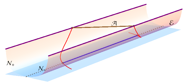
Figure 11: In this figure the interval $\mathcal{A}$ is on the cutoff boundary $r=r_{I}$ and its endpoints $\partial_{\pm}\mathcal{A}$ are on $\mathcal{N}_{\pm}$. The two red lines are the two null geodesics (5.74) which intersect with $\mathcal{E}$ at the endpoints of $\mathcal{E}_{reg}$ (the solid blue line).

6 Towards the generalized gravitational entropy for spacetimes with non-Lorentz duals

Based on the above discussions, we are ready to generalize our intrinsic prescription to calculate the generalized gravitational entropy for general spacetimes with non-Lorentz invariant duals. As expected the prescription only evolves extremal surfaces $\mathcal{E}$ and their associated normal null hypersurfaces $\mathcal{N}_{\pm}$, which are available when the bulk metric is given.

For a bulk spacetime $\mathcal{M}$ and its asymptotic boundary $\mathcal{B}$ at $r\to\infty$, when a holography is conjectured between the bulk gravity theory (here we only consider Einstein gravity) and the field theory on $\mathcal{B}$. The prescription is in the following

1. Firstly we should figure out the causal structure of the boundary field theory, using either the boundary null geodesics (or hypersurfaces) when the metric background is fixed, or the Rindler method. In other words, for a given subregion $\mathcal{A}$ we should find out the corresponding causal development $\mathcal{D}_{\mathcal{A}}$. For non-Lorentzian field theories, the causal developments usually looks like a strip (or a solid cylinder) rather than a diamond.

2. For a general spacelike extremal surface we study its normal null hypersurfaces $\mathcal{N}_{\pm}$. As we have discussed before, the $\mathcal{E}$ can be determined by following requirement

   $$\mathcal{E}:~{}\mathcal{N}_{\pm}\cap\mathcal{B}\supset\partial\mathcal{D}_{\mathcal{A}}\,,$$ (6.76)

   which is just the requirement for the consistency between the bulk and boundary causal structures.

3. Then we push the dual field theory to the cutoff boundary at some large radius $r=r_{I}$ . During we push the boundary, it is crucial how the entangling surface $\partial\mathcal{A}$ moves. The main requirement is that $\partial\mathcal{A}$ should adapt to the consistency of the bulk and boundary causal structures on $r=r_{I}$. For the cases with non-Lorentz invariant duals, we should keep $\partial\mathcal{A}$ on $\mathcal{N}_{\pm}$ and keep the coordinates, whose UV cutoff can be taken to be zero, fixed.

4. On $\mathcal{N}_{\pm}$, there are null geodesics $\gamma_{\pm}$ (or codimension two null hypersufaces) emanating from $\partial\mathcal{A}$ at the cutoff boundary $r=r_{I}$. We cut off the extremal surface $\mathcal{E}$ at the place where $\gamma_{\pm}$ intersect with $\mathcal{E}$. Then we get the regulated extremal surface $\mathcal{E}_{reg}$ and the regulated holographic entanglement entropy

   $$S_{\mathcal{A}}=\frac{Area\left(\mathcal{E}_{reg}\right)}{4G}\,.$$ (6.77)

The first two steps show how to use the consistency of the causual structures to determine the $\mathcal{E}$ corresponding to the boundary subregion $\mathcal{A}$ in question, while the last two steps tell us how to regulate $\mathcal{E}$ using the null geodesics on $\mathcal{N}_{\pm}$. We conjuecture that way we push $\partial\mathcal{A}$ will get it to the right modular plane that determines the regulation.

For the cases with locally defined modular Hamiltonian, the fine structure analysis with the modular planes gives a strong support for the validity of our prescription. However in more general cases, the modular Hamiltonian is usually non-local, so the modular planes can no longer be described as certain bulk codimension one surfaces. Instead they should be defined in a more abstract way. We would like to stress that, for the more general cases our prescription is still applicable. Though in general the modular Hamiltonian is non-local, effectively it can be locally defined in some special bulk and boundary regions: the region near the $\mathcal{N}_{\pm}$ and the region near $\partial\mathcal{D}_{\mathcal{A}}$. This indicates the modular planes can also be locally defined in these regions and intersect with $\mathcal{N}_{\pm}$ on the null geodesics that form $\mathcal{N}_{\pm}$. Note that our prescription is insensitive to how the modular planes look like outside these regions, so with all the geometric quantities (including the cutoff points of $\mathcal{A}$, the extremal surface $\mathcal{E}$ and the null geodesics or hypersurfaces $\gamma_{\pm}$ on $\mathcal{N}_{\pm}$) we need to apply our prescription inside these regions, our prescription is still applicable. We conjecture that the result we get by applying our prescription is still the right holographic entanglement entropy.

In the following we give an argument for this statement. When we need to do the regulation, we can divide the $\mathcal{A}$ and $\mathcal{E}$ into two parts

$$\mathcal{A}=\mathcal{A}_{cut}\cup\mathcal{A}_{reg}\,,\qquad\mathcal{E}=\mathcal{E}_{cut}\cup\mathcal{E}_{reg}.$$ (6.78)

Here $\mathcal{A}_{cut}$ is the infinitesimal part of $\mathcal{A}$ we cut off. Also the total entanglement entropy can be divided into two parts which are contributed from $\mathcal{A}_{cut}$ and $\mathcal{A}_{reg}$ respectively

$$S_{\mathcal{A}}=s_{\mathcal{A}}({\mathcal{A}_{cut}})+s_{\mathcal{A}}({\mathcal{A}_{reg}})=\frac{Area(\mathcal{E})}{4G}\,.$$ (6.79)

Though the fine correspondence for the points on $\mathcal{A}_{reg}$ no longer exists when the modular Hamiltonian is non-local, it still holds between the points on $\mathcal{A}_{cut}$ and the points on $\mathcal{E}_{cut}$. This is because $\mathcal{A}_{cut}$ is in the near $\partial\mathcal{D}$ region, where the modular flow effectively has a local description. So according to the fine correspondence $\mathcal{A}_{cut}$ correspond to some part of $\mathcal{E}$ which we call $\mathcal{E}_{cut}$, such that

$$s_{\mathcal{A}}({\mathcal{A}_{cut}})=\frac{Area(\mathcal{E}_{cut})}{4G}\,.$$ (6.80)

Together with (6.79), we find the regulated entanglement entropy is given by

$$S_{\mathcal{A}}^{reg}=s_{\mathcal{A}}({\mathcal{A}_{reg}})=\frac{Area(\mathcal{E}_{reg})}{4G}\,.$$ (6.81)

7 Generalised gravitational entropy for 3-dimensional flat space

In this section we apply our prescription to the case of 3-dimensional flat holography Barnich:2010eb ; Bagchi:2010eg ; Bagchi:2012cy . In this holography, the 3-dimensional asymptotic flat spacetime is conjectured to be dual to a field theory invariant under the BMS₃ group (BMSFT). The BMS₃ group is the asymptotic symmetry group of flat space enhanced from the Poincaré group, and the BMSFT can be considered as the ultra-relativistic limit of a CFT₂. The holographic calculation, as well as the geometric picture, of the entanglement entropy for BMSFTs are given in Jiang:2017ecm with the Rindler method. We will show that our prescription can easily reproduce the results in Jiang:2017ecm without the Rindler transformations and modular flows.

In particular we consider the following classical solutions of Einstein gravity with vanishing cosmological constant in Bondi gauge

$$ds^{2}=Mdu^{2}-2dudr+Jdud\phi+r^{2}d\phi^{2}.$$ (7.82)

The above solutions are usually classified into three types:

• $M=-1,J=0$: Global Minkowski, which duals to the zero temperature BMSFT on the cylinder with $\phi\sim\phi+2\pi$.

• $M=J=0$: Null-orbifold, with $\phi$ decompactified this duals to the zero temperature BMSFT on the plane.

• $M>0$: Flat Space Cosmological solutions (FSC), which duals to BMSFT at finite temperature.

The asymptotic boundary (null infinity) $\mathcal{B}$ settles at $r=r_{I}\to\infty$ with a fixed background metric

$$ds^{2}=0du^{2}+d\phi^{2}\,,$$ (7.83)

which is degenerate. On $\mathcal{B}$ the null direction is characterized by $u$. The subregion we study is a single interval

$$\mathcal{A}:\qquad(-l_{u}/2,-l_{\phi}/2)\rightarrow(l_{u}/2,l_{\phi}/2)\,.$$ (7.84)

Since $u$ is the null direction, the domain of causality $\mathcal{D}_{\mathcal{A}}$ is just a strip along the $u$ direction

$$\mathcal{D}_{\mathcal{A}}:\qquad\{-\frac{l_{\phi}}{2}\leq\phi\leq\frac{l_{\phi}}{2}\}\,.$$ (7.85)

Asymptotically we should have

$$\partial\mathcal{D}_{\mathcal{A}}:\qquad\phi=\pm\frac{l_{\phi}}{2}+\mathcal{O}\left(\frac{1}{r_{I}}\right)\,,\qquad r=r_{I}\,.$$ (7.86)

It will be quite subtle to apply our prescription in the Bondi gauge, so we apply it in the Cartesian coordinates. Another advantage of using the Cartesian coordinates is that we do not need to solve the Einstein equations, because the geodesics and their null normal hypersurfaces are just straight lines and null planes.

7.1 Null-orbifold

We choose the coordinate transformation between the Null-orbifold and the Cartesian coordinates to be

$$t ={l_{\phi}\over 4}r+{2\over l_{\phi}}(u+\frac{r\phi^{2}}{2})\,,$$ (7.87)

$$x =({l_{u}\over l_{\phi}}+r\phi)\,,$$ (7.88)

$$y ={l_{\phi}\over 4}r-{2\over l_{\phi}}(u+\frac{r\phi^{2}}{2})\,.$$ (7.89)

Here we have adjusted the transformation in advance by some proper Poincaré transformation and the coefficients are chosen to be related to the parameters $l_{u}$ and $l_{\phi}$ which characterize the boundary interval $\mathcal{A}$, hence the curve $\mathcal{E}$ can be characterized by a single coordinate $y$ and settled at $t=x=0$. Of course one can begin with free coefficients and settle them down one by one through the matching condition (2.6). It is easy to check that, up to a Poincaré transformation for the Cartesian coordinates, we have

$$ds^{2} =-2dudr+r^{2}d\phi^{2}=-dt^{2}+dx^{2}+dy^{2}\,.$$ (7.90)

Then in Cartesian coordinates $\partial\mathcal{D}_{\mathcal{A}}$ (7.86) and the two endpoints $\partial_{\pm}\mathcal{A}$ of $\mathcal{A}$ are given by

$$\partial\mathcal{D}_{\mathcal{A}}: \quad\left\{t,x,y\right\}=\left\{\frac{l_{\phi}}{2}r_{I}+\mathcal{O}\left(r_{I}^{0}\right),\pm\frac{l_{\phi}}{2}r_{I}+\mathcal{O}\left(r_{I}^{0}\right),-\frac{2u}{l_{\phi}}\right\}\,,$$ (7.91)

$$\partial_{\pm}\mathcal{A}: \quad\left\{t,x,y\right\}=\left\{\frac{l_{\phi}}{2}r_{I}\pm\frac{l_{u}}{l_{\phi}},\pm\frac{l_{\phi}}{2}r_{I}+\frac{l_{u}}{l_{\phi}},\mp\frac{l_{u}}{l_{\phi}}\right\}\,.$$ (7.92)

It is easy to see that the spacelike geodesic $\mathcal{E}$ and the associated $\mathcal{N}_{\pm}$ that asymptotically satisfy (2.6) are just given by

$$\mathcal{E}: \quad\left\{x=0,\quad t=0\right\}\,,$$ (7.93)

$$\mathcal{N}_{\pm}: \quad\left\{x=\pm t\right\}\,.$$ (7.94)

Obviously $\mathcal{N}_{\pm}$ (7.94) will asymptotically go through $\partial\mathcal{D}_{\mathcal{A}}$ (7.91).

Then we regulate $\mathcal{E}$ using null geodesics on $\mathcal{N}_{\pm}$. The two null geodesics $\gamma_{\pm}$ on $\mathcal{N}_{\pm}$ that emanating from $\partial_{\pm}\mathcal{A}$ are given by

$$\gamma_{\pm}:\quad\left\{x=\pm t\,,\quad y=\mp\frac{l_{u}}{l_{\phi}}\right\}\,.$$ (7.95)

Note that in this case there is no need to introduce UV cutoffs in the $u$ and $\phi$ direction since they can be taken to be zero without introducing divergence to the entanglement entropy. So when we push the boundary, we keep the $u$ sand $\phi$ coordinate of $\partial_{\pm}\mathcal{A}$ fixed. This means $\partial_{\pm}\mathcal{A}$ moves along $\gamma_{\pm}$ and the $\mathcal{E}_{reg}$ will be independent of the choice of $r_{I}$. The overall picture of our construction is shown in Fig. 12.

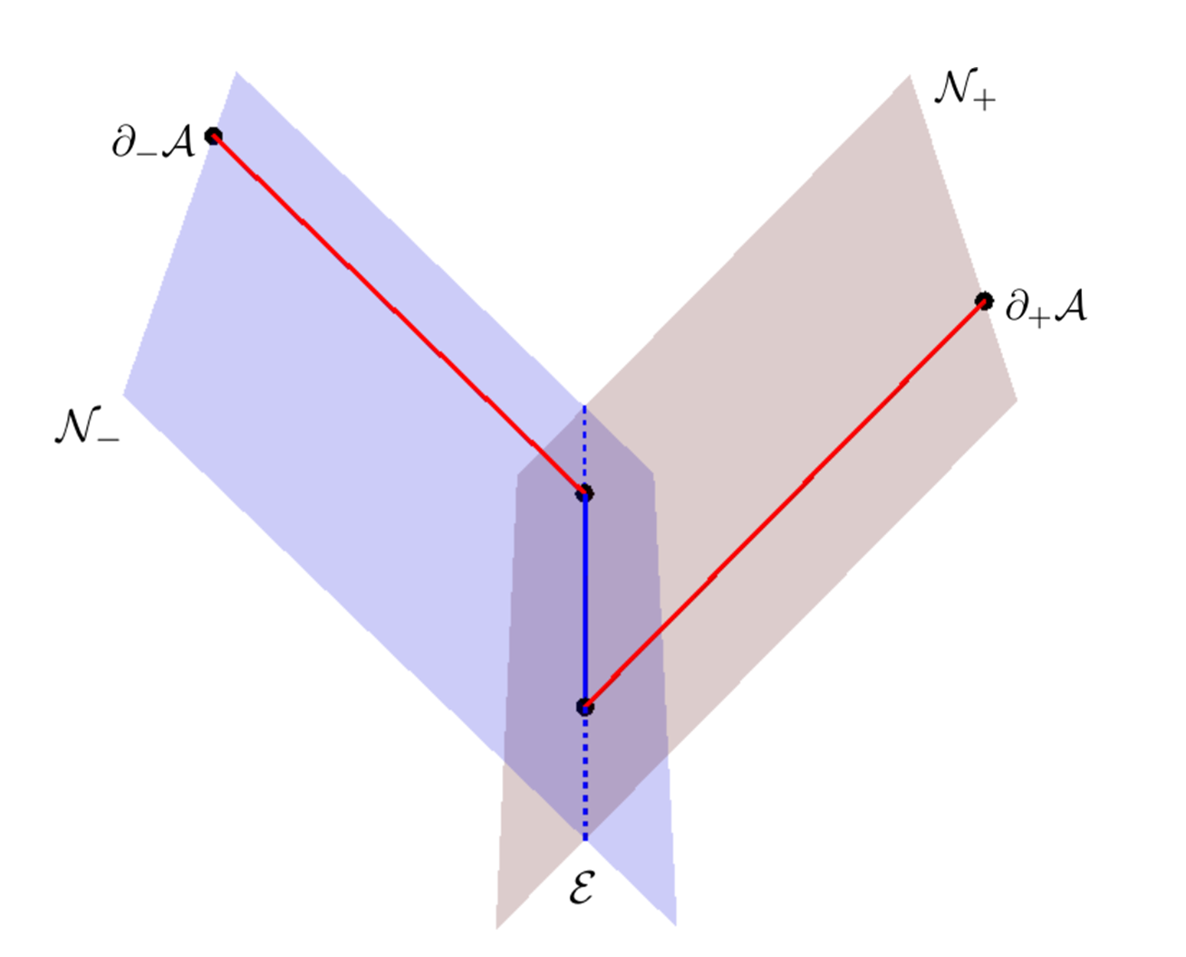
Figure 12: The two red lines are the null rays $\gamma_{\pm}$ emanating from $\partial_{\pm}\mathcal{A}$ and normal to $\mathcal{E}$. The geodesic $\mathcal{E}$ is cut off where it intersect with $\gamma_{\pm}$. The solid blue segment is just our $\mathcal{E}_{reg}$.

According to our prescription, the points where $\gamma_{\pm}$ intersect with $\mathcal{E}$ are the place we cut $\mathcal{E}$ off. Then we get

$$\mathcal{E}_{reg}:\quad\left\{x=t=0\,,\quad-\frac{l_{u}}{l_{\phi}}\leq y\leq\frac{l_{u}}{l_{\phi}}\right\}\,.$$ (7.96)

Accordingly we have

$$S_{\mathcal{A}}=\frac{Area\left(\mathcal{E}_{reg}\right)}{4G}=\frac{1}{2G}\frac{l_{u}}{l_{\phi}}\,,$$ (7.97)

which reproduces the results in Bagchi:2014iea ; Basu:2015evh ; Jiang:2017ecm ; Hijano:2017eii .

7.2 Global Minkowski

The global Minkowski space

$$ds^{2}=-du^{2}-2dudr+r^{2}d\phi^{2}\,,$$ (7.98)

can be transformed to the Cartesian coordinates by the following transformation

$$t= (r+u)\csc\frac{l_{\phi}}{2}+\frac{r\cos\phi}{2}\left(\tan\frac{l_{\phi}}{4}-\cot\frac{l_{\phi}}{4}\right)\,,$$ (7.99)

$$x= r\sin\phi+\frac{1}{2}l_{u}\csc\frac{l_{\phi}}{2}\,,$$ (7.100)

$$y= r\cos\phi\csc\frac{l_{\phi}}{2}-(r+u)\cot\frac{l_{\phi}}{2}\,.$$ (7.101)

Then in Cartesian coordinates we have

$$\partial\mathcal{D}_{\mathcal{A}}: \quad\left\{t,x,y\right\}=\left\{\sin\frac{l_{\phi}}{2}r_{I}+\mathcal{O}\left(r_{I}^{0}\right),\pm\sin\frac{l_{\phi}}{2}r_{I}+\mathcal{O}\left(r_{I}^{0}\right),-u\cot\frac{l_{\phi}}{2}\right\}$$ (7.102)

$$\partial_{\pm}\mathcal{A}: \quad\left\{t,x,y\right\}=\left\{\frac{\csc\frac{l_{\phi}}{2}}{2}\left(l_{u}\pm 2r_{I}\sin^{2}\frac{l_{\phi}}{2}\right),\pm r_{I}\sin\frac{l_{\phi}}{2},\mp\frac{l_{u}\cot\frac{l_{\phi}}{2}}{2}\right\}$$ (7.103)

Similarly we get the spacelike geodesic $\mathcal{E}$ and the associated $\mathcal{N}_{\pm}$ that asymptotically satisfy the requirement (2.6)

$$\mathcal{E}: \quad\left\{x=0,\quad t=0\right\}\,,$$ (7.104)

$$\mathcal{N}_{\pm}: \quad\left\{x=\pm t\right\}\,.$$ (7.105)

The two null geodesics $\gamma_{\pm}$ on $\mathcal{N}_{\pm}$ that emanating from $\partial_{\pm}\mathcal{A}$ are just given by

$$\gamma_{\pm}:\quad\left\{x=\pm t\,,\quad y=\mp l_{u}\cot\frac{l_{\phi}}{2}\right\}\,.$$ (7.106)

Quite straightforwardly we get

$$S_{\mathcal{A}}=\frac{Area\left(\mathcal{E}_{reg}\right)}{4G}=\frac{l_{u}}{2G}\cot\frac{l_{\phi}}{2}\,.$$ (7.107)

7.3 Flat Space Cosmological solutions

The coordinate transformations from FSC to the Minkowski space can be given by

$$r =\sqrt{M(t^{\prime 2}-x^{\prime 2})+r_{c}^{2}}\,,$$ (7.108)

$$\phi =-\frac{1}{\sqrt{M}}\log\frac{\sqrt{M}(t^{\prime}-x^{\prime})}{r+\frac{J}{2\sqrt{M}}}\,,$$ (7.109)

$$u =\frac{1}{M}\Big{(}r-\sqrt{M}y^{\prime}-\frac{J}{2}\phi\Big{)}\,.$$ (7.110)

The above transformations show that the FSC can be considered as a quotient of the Minkowski space, because the region outside the cosmological horizon $r_{c}=\frac{J}{2\sqrt{M}}$ only covers a quarter of the Minkowski space $t^{\prime}\geq|x^{\prime}|$.

As in the previous two cases, we can apply an additional Poincaré transformation to a new set of Cartesian coordinates $\{t,x,y\}$ thus the corresponding $\mathcal{E}$ and $\mathcal{N}_{\pm}$ are just given by (7.93) and (7.94). Under this requirement $\partial\mathcal{D}_{\mathcal{A}}$ (7.86) should asymptotically satisfy $t=\pm x$, then we find that the additional Poincaré transformation is just

$$t= t^{\prime}\cosh\eta-y^{\prime}\sinh\eta\,,$$ (7.111)

$$x= x^{\prime}+s_{0}\,,$$ (7.112)

$$y= y^{\prime}\cosh\eta-t^{\prime}\sinh\eta\,,$$ (7.113)

where

$$\eta=\text{arccosh}\left[\text{coth}\frac{l_{\phi}\sqrt{M}}{2}\right]\,,\qquad s_{0}=\frac{(Jl_{\phi}+2l_{u}M)\text{csch}\frac{l_{\phi}\sqrt{M}}{2}}{4\sqrt{M}}\,.$$ (7.114)

Then in Cartesian coordinates we have

$$\partial\mathcal{D}_{\mathcal{A}}: \quad\left\{t,x,y\right\}=\Big{\{}\frac{\sinh\frac{l_{\phi}\sqrt{M}}{2}}{\sqrt{M}}r_{I}+\mathcal{O}\left(r_{I}^{0}\right),\pm\frac{\sinh\frac{l_{\phi}\sqrt{M}}{2}}{\sqrt{M}}r_{I}+\mathcal{O}\left(r_{I}^{0}\right),$$ (7.115)

$$~{}~{}~{}~{}~{}~{}~{}~{}~{}~{}~{}~{}~{}~{}~{}~{}~{}~{}~{}~{}~{}\frac{\pm 2J\mp\sqrt{M}\left(Jl_{\phi}\pm 4Mu\right)\coth\frac{l_{\phi}\sqrt{M}}{2}}{4M}\Big{\}}\,,$$ (7.116)

$$\partial_{\pm}\mathcal{A}: \quad y=\frac{\pm 2J\mp\sqrt{M}\coth\left(\frac{\sqrt{M}l_{\phi}}{2}\right)\left(Jl_{\phi}\pm 2Ml_{u}\right)}{4M}\,.$$ (7.117)

For simplicity we only list the $y$ coordinates of $\partial_{\pm}\mathcal{A}$. The two null geodesics $\gamma_{\pm}$ emanating from $\partial_{\pm}\mathcal{A}$ are given by

$$\gamma_{\pm}:\quad\Big{\{}x=\pm t\,,\quad y=\frac{\pm 2J\mp\sqrt{M}\coth\left(\frac{\sqrt{M}l_{\phi}}{2}\right)\left(Jl_{\phi}\pm 2Ml_{u}\right)}{4M}\Big{\}}\,.$$ (7.118)

Again we reproduce the right result

$$S_{\mathcal{A}}=\frac{Area\left(\mathcal{E}_{reg}\right)}{4G}=\frac{1}{4G}\left|\frac{\left(Jl_{\phi}+2Ml_{u}\right)}{2\sqrt{M}}\coth\left(\frac{\sqrt{M}l_{\phi}}{2}\right)-\frac{J}{M}\right|\,.$$ (7.119)

8 Discussion

In this paper we demonstrate how the RT formula fails to give the geometric picture of the holographic entanglement entropy for spacetimes with non-Lorentz invariant duals. We extend the discussion of Lewkowycz:2013nqa to holographies beyond AdS/CFT. The two main points which are crucial for this extension include the requirement for the consistency between the bulk and boundary causal structures, and the introduction of null geodesics (or hypersurfaces) to control the regulation of entanglement entropy. Since $\gamma_{\pm}$ are null thus do not contribute to the total length, one may consider a new $\mathcal{E}=\mathcal{E}_{reg}\cup\gamma_{+}\cup\gamma_{-}$ such that $\mathcal{E}$ is anchored on $\partial\mathcal{A}$ as the RT formula. However we do not suggest to do that. First of all, $\mathcal{E}_{reg}$ is fixed under the modular flow (or replica symmetry) while $\gamma_{\pm}$ are not. So they play totally different roles in the replica story. Also they play different roles in the new extrapolate dictionary (8.120) which we will discuss later. Secondly, the requirement that the new $\mathcal{E}$ is anchored on $\partial\mathcal{A}$ does not help to determine the geometric picture as the RT formula, because usually the null geodesics emanating from $\partial\mathcal{A}$ are not unique. So we still need the help of (2.6) to determine $\mathcal{E}$. At last, unlike $\mathcal{E}$, the null geodesics $\gamma_{\pm}$ depend on the cutoff $\epsilon$.

Since the RT formula stimulates numerous insights in our understanding of the AdS/CFT in many aspects, we expect the parallel discussions based on our prescription can help us to better understand the holographies beyond AdS/CFT. In the following we list a few interesting problems that may be solved based on our new geometric picture.

Holographic entanglement entropy for Lifshitz spacetime

One particular interesting class of non-Lorentzian field theories are those with Lifshitz symmetries. The dual spacetime, which we call Lifshitz spacetimes, was proposed in Kachru:2008yh ; Taylor:2015glc . It has been shown in Gentle:2015cfp that the normal null hypersurfaces emanating from the RT (or HRT) surface in Lifshitz spacetime can not reach the boundary and thus fail to satisfy (2.6). This implies the inconsistency between the bulk and boundary casual structures, so the RT formula should fail in this case according to our discussion. This means the calculations of the holographic entanglement entropies for Lifshitz-type theories lif1 ; lif2 ; lif3 ; lif4 ; lif6 ; lif7 ; lif8 ; lif9 following the RT formula should not be correct. Also they are not consistent with the recent numerical results Nlif1 ; Nlif2 ; Nlif3 ; Nlif4 of entanglement entropies for free Lifshitz-type theories.

Assuming the gravity dual is an Einstein gravity, our prescription can be applied to the Lifshitz spacetimes and give new holographic predictions for the entanglement entropy of holographic Lifshitz-type theories. Also it is argued in Griffin:2012qx that Horava-Lifshitz gravity is the minimal holographic dual for Lifshitz field theories (see also Cheyne:2017bis along this line). In this case our prescription need corrections.

Holographic entanglement entropy in higher dimensional flat space

The geometric picture for holographic entanglement entropy in 3-dimensional flat holography is carried out in Jiang:2017ecm by Rindler method. It is then straightforward to ask whether we can extend the calculation to the case of flat holography in 4-dimensions, which has recently attracted lots of attention (see Strominger:2017zoo for a recent review). Unfortunately the Rindler method get much more complicated in higher dimensions. Since the prescription proposed in this paper is intrinsic and has natural extension to higher dimensions, it will be more promising to solve this problem by our prescription.

New extrapolate dictionary between boundary operators and bulk matter fields

Following the replica trick, the entanglement entropy in a field theory can be computed by evaluating the two point function of twist operators located at the boundary endpoints. So the new geometric picture of entanglement entropy with extra null geodesics gives a new holographic description for the two point correlation functions. Motivated by this picture and a similar prescription Hijano:2015rla ; Castro:2017hpx for calculating holographic conformal blocks in the probe limit in AdS/CFT, the authors of Hijano:2017eii calculated the Poincaré blocks (or global BMS blocks) for BMSFT holographically by extremizing the length of a network of geodesics connected to the operators at the boundary through certain null geodesics. And the results match with the calculations Bagchi:2017cpu on the field theory side.

Based on the above results, an extrapolate dictionary is proposed in Hijano:2017eii (see also Hijano:2018nhq ) for flat holography. More explicitly, to each boundary point $x$ where we inject an operator, we attach a null line $\gamma_{x}$, which is similar to the null lines $\gamma_{\pm}$ in our geometric picture for entanglement entropy. The proposed extrapolate dictionary is then to attach a position space Feynman diagram to the null lines and integrate the position of the legs over an affine parameter along $\gamma_{x}$

$$\left<\mathcal{O}(x_{1})\mathcal{O}(x_{2})\cdots\right>=\int_{\gamma_{x_{1}}}d\lambda_{1}\int_{\gamma_{x_{2}}}d\lambda_{2}\cdots\left<\psi(\lambda_{1})\psi(\lambda_{2})\cdots\right>\,.$$ (8.120)

Here $\psi$ denotes the bulk matter fields that correspond to the boundary operators $\mathcal{O}$, and $\lambda_{i}$ parametrizes the null geodesic $\gamma_{x_{i}}$ emanating from the boundary point $x_{i}$. The above extrapolate dictionary in flat holography is totally different from the one Witten:1998qj in AdS/CFT, and gives another entry to study flat holography.

Our analysis shows that the geometric picture for holographic entanglement entropy in spacetimes with non-Lorentzian duals should in general include the extra null geodesics (or null hypersurfaces). So in these cases, the right extrapolate dictionary for boundary operators and bulk matter fields should be similar to (8.120) rather the one Witten:1998qj in AdS/CFT. It will be very interesting to test the dictionary (8.120) and calculate the correlation functions holographically in other spacetimes with non-Lorentz invariant duals.

Acknowledgments

We would like to thank Wei Song and Rong-xin Miao for initial collaboration on this project and insightful discussions. We thank Matthew Headrick and Hongliang Jiang for helpful discussions. We thank Wei Song, Chang-pu Sun, Pin Yu, Wenbin Yan and the Yau Mathematical Sciences Center of Tsinghua University for support. We would also like to thank the Center of Mathematical Sciences and Applications at Harvard University for hospitality during the development of this work. This work is supported by NSFC Grant No.11805109.

Appendix A Spacelike geodesics in AdS₃

The spacelike geodesics in the AdS₃ (3.9) with $T_{u}=0$ satisfy the following equations of motion

$$\frac{c_{1}}{\ell^{2}} =r\dot{v}\,,$$ (A.121)

$$\frac{c_{2}}{\ell^{2}} =r\dot{u}+T_{v}^{2}\dot{v}\,,$$ (A.122)

$$\frac{1}{\ell^{2}} =T_{v}^{2}\dot{v}^{2}+2r\dot{u}\dot{v}+\frac{\dot{r}^{2}}{4r^{2}}\,,$$ (A.123)

where we $c_{1}$ and $c_{2}$ are two integration constants, satisfying $c_{1}c_{2}>0$, and dot represent differential with respect to the affine parameter $s$. From (A.121) and (A.122) we get

$$\dot{u}={c_{2}r-c_{1}T_{v}^{2}\over\ell^{2}r^{2}}\,,\qquad\dot{v}={c_{1}\over r\ell^{2}}\,.$$ (A.124)

Substituting the above equations into (A.123) we get a radial equation

$$\dot{r}=\pm\frac{2\sqrt{r\left(\ell^{2}r-2c_{1}c_{2}\right)+T_{v}^{2}c_{1}^{2}}}{\ell}\,,$$ (A.125)

We get three types of spacelike geodesics by adjusting the value of $|c_{2}|$. Firstly when

$$|c_{2}|>\ell T_{v}\,,$$ (A.126)

we find $\dot{r}=0$ at

$$r_{\pm}=\frac{c_{1}c_{2}\pm\sqrt{c_{1}^{2}\left(c_{2}^{2}-\ell^{2}T_{v}^{2}\right)}}{\ell^{2}}>0\,.$$ (A.127)

This type of geodesic is anchored on the boundary and has a turning points at $r_{+}$, thus belongs to the RT curves. The second type of geodesic satisfies $|c_{2}|<\ell T_{v}$ thus has no turning points.

Both of the above two types do not satisfy our requirement (2.6). The third type of geodesic that never touches the boundary arises when

$$|c_{2}|=\ell T_{v}\,.$$ (A.128)

In this case we find that, at $r={c_{1}T_{v}\over\ell},$

$$\dot{r}=\dot{u}=0,\qquad\dot{v}={1\over c_{2}}=\pm{1\over\ell T_{v}}\,.$$ (A.129)

The corresponding geodesics $\mathcal{E}$ lies along the $v$ direction at a fixed radius

$$\mathcal{E}:~{}~{}\{r=\frac{c_{1}T_{v}}{\ell}\,,\quad u=u_{0}\}\,,$$ (A.130)

where $u_{0}$ is an arbitrary constant. In the case (3.16) we study, we set $T_{v}=1$. Note that, for our coordinates (3.9), the global AdS correspond to $T_{u}=T_{v}=\frac{i}{2}$ and Poincaré AdS correspond to $T_{u}=T_{v}=0$. In these two cases there are no spacelike geodesics that do not touch the boundary. For the given interval (3.17), the $\mathcal{E}$ that satisfies the requirement (2.6) is just (A.130) with $c_{1}=\frac{1}{l_{u}}$.

Appendix B Entanglement contour for WCFT

B.1 Entanglement contour from the fine structure

The entanglement contour function is a density function of entanglement. In other words it describes the distribution of the contribution to the total entanglement entropy from each point of $\mathcal{A}$

$$S_{\mathcal{A}}=\int_{\mathcal{A}}s_{\mathcal{A}}(v)dv\,.$$ (B.131)

Here we parametrize $\mathcal{A}$ with the $v$ coordinate. The authors of Vidal proposed a set of requirements for the contour functions. Few analysis of the contour functions for bipartite entanglement have been explored in Botero ; Vidal ; PhysRevB.92.115129 ; Coser:2017dtb ; Tonni:2017jom . Also its fundamental definition is still not established.

In the previous section we propose that $Length(\mathcal{E}_{2})$ captures the contribution from $\mathcal{A}_{2}$ to the entanglement entropy $S_{\mathcal{A}}$. In other words our fine structure analysis gives a holographic interpretation for the contour function. Consider $\mathcal{A}$ to be a straight line (5.66), according to the fine correspondence (5.67) we get the contour function $s_{\mathcal{A}}(v)$ for $S_{\mathcal{A}}$

$$s_{\mathcal{A}}(v)=\frac{1}{4G}\left(1+\frac{2l_{v}}{l_{v}^{2}-4v^{2}}\right)\,.$$ (B.132)

Let us define

$$s_{\mathcal{A}}(\mathcal{A}_{2})=\int_{\mathcal{A}_{2}}s_{\mathcal{A}}(v)dv=\frac{Length(\mathcal{E}_{2})}{4G}\,.$$ (B.133)

According to the fine correspondence (5.67) or the contour function (B.132), we have

$$s_{\mathcal{A}}(\mathcal{A}_{2})=\frac{1}{4G}\left(v^{\prime}_{2}-v^{\prime}_{1}+\text{arctanh}\frac{2v^{\prime}_{2}}{l_{v}}-\text{arctanh}\frac{2v^{\prime}_{1}}{l_{v}}\right)$$ (B.134)

where $v^{\prime}_{1}$ and $v^{\prime}_{2}$ are the $v$ coordinates of the two endpoints of $\mathcal{A}_{2}$.

Furthermore we consider two intervals $\mathcal{A}$ and $\mathcal{A}^{\prime}$ that have the same causal development $\mathcal{D}_{\mathcal{A}}=\mathcal{D}_{\mathcal{A}^{\prime}}$. The two arbitrary boundary modular flow lines $\mathcal{L}_{v_{1}}$ and $\mathcal{L}_{v_{2}}$ that divide $\mathcal{A}$ ($\mathcal{A}^{\prime}$) into three part $\mathcal{A}_{1},\mathcal{A}_{2}$ and $\mathcal{A}_{3}$ ($\mathcal{A}^{\prime}_{1},\mathcal{A}^{\prime}_{2}$ and $\mathcal{A}^{\prime}_{3}$). See Fig.13. According to our prescription, any $\mathcal{A}_{2}$ that goes through the same bunch of modular planes should correspond to the same $\mathcal{E}_{2}$ on $\mathcal{E}$. Then we should have the following causal property for $S_{\mathcal{A}}(\mathcal{A}_{2})$

$$S_{\mathcal{A}}(\mathcal{A}_{2})=\mathcal{S}_{\mathcal{A}^{\prime}}(\mathcal{A}^{\prime}_{2})\,.$$ (B.135)

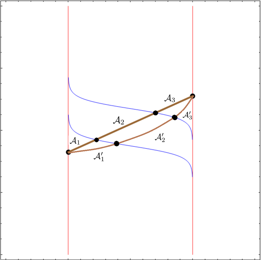
Figure 13: The two blue lines are two modular flow lines $\mathcal{L}_{v_{1}}$ and $\mathcal{L}_{v_{2}}$ on the boundary. Here $\mathcal{A}_{2}$ and $\mathcal{A}^{\prime}_{2}$ intersect with the same bunch of modular planes between $\mathcal{P}(v_{1})$ and $\mathcal{P}(v_{2})$.

B.2 Testing the entanglement contour proposal

It is proposed in Wen:2018whg that in general theories the $s_{\mathcal{A}}(\mathcal{A}_{2})$ can be written as a linear combination of the entanglement entropies of single subintervals inside $\mathcal{A}$

$$s_{\mathcal{A}}(\mathcal{A}_{2}) =\frac{1}{2}\left(S_{\mathcal{A}_{1}\cup\mathcal{A}_{2}}+S_{\mathcal{A}_{2}\cup\mathcal{A}_{3}}-S_{\mathcal{A}_{1}}-S_{\mathcal{A}_{3}}\right)\,.$$ (B.136)

Here we would like to test this proposal for WCFT. Using (5.71) for all these sub-intervals on the straight interval $\mathcal{A}$ (5.66) we have

$$s_{\mathcal{A}}(\mathcal{A}_{2}) =\frac{c}{6}\left(v^{\prime}_{2}-v^{\prime}_{1}+\frac{1}{2}\log\frac{(v^{\prime}_{2}+\frac{l_{v}}{2})(v^{\prime}_{1}-\frac{l_{v}}{2})}{(v^{\prime}_{2}-\frac{l_{v}}{2})(v^{\prime}_{1}+\frac{l_{v}}{2})}\right)=\frac{c}{6}(v_{2}-v_{1})\,,$$ (B.137)

which coincide with the result (B.134) we get from the entanglement contour (B.132).

Then we test the causal property (B.135) for the proposal (B.136). We let the two endpoints of $\mathcal{A}_{2}$ run along the boundary modular flow lines $\mathcal{L}_{v_{1}}$ and $\mathcal{L}_{v_{2}}$ that passing trough them (see Fig. 13),

$$(u^{\prime}_{1},v^{\prime}_{1})=(u^{\prime}_{1},v_{1}-\text{arctanh}\frac{2u^{\prime}_{1}}{l_{u}})\,,$$ (B.138)

$$(u^{\prime}_{2},v^{\prime}_{2})=(u^{\prime}_{2},v_{2}-\text{arctanh}\frac{2u^{\prime}_{2}}{l_{u}})\,,$$ (B.139)

The new subinterval $\mathcal{A}^{\prime}_{2}$ passes through the same class of modular planes as $\mathcal{A}_{2}$, so satisfy (B.135). With all the endpoints of subintervals known, we apply (5.71) and find

$$S_{\mathcal{A}^{\prime}_{1}\cup\mathcal{A}^{\prime}_{2}}+S_{\mathcal{A}^{\prime}_{2}\cup\mathcal{A}^{\prime}_{3}}-S_{\mathcal{A}^{\prime}_{1}}-S_{\mathcal{A}^{\prime}_{3}} =\frac{c}{3}\left(v_{2}-v_{1}\right)$$ (B.140)

$$=S_{\mathcal{A}_{1}\cup\mathcal{A}_{2}}+S_{\mathcal{A}_{2}\cup\mathcal{A}_{3}}-S_{\mathcal{A}_{1}}-S_{\mathcal{A}_{3}}\,.$$ (B.141)

This indicates that the linear combination in (B.136) reproduce the right causal property for the contour function.

Appendix C The saddle that connect the two null curves $\gamma_{\pm}$

Here we prove that the regulated curve $\mathcal{E}_{reg}$ is the saddle among all the geodesics that connect $\gamma_{\pm}$ (5.74). To prove this we need to calculate the proper distances between arbitrary two points in the bulk, then we fix the endpoints on $\gamma_{+}$ and $\gamma_{-}$ respectively and find out the saddle among all the geodesics. It is easier to start from calculating the proper length of arbitrary two points in Poincaré AdS, then we rewrite the distance in terms of the variables in the AdS space with nonzero temperatures via a coordinate transformation.

For simplicity we consider the Poincaré AdS₃ spacetime

$$ds^{2}=\ell^{2}\Big{(}\frac{d\rho^{2}}{4\rho^{2}}+2\rho dUdV\Big{)}\,.$$ (C.142)

with the geodesics given by

$$U= \frac{l_{U}}{2}\tanh\tau+c_{U}\,,\qquad V=\frac{l_{V}}{2}\tanh\tau+c_{V}\,,\qquad\rho=\frac{2\cosh^{2}\tau}{l_{U}l_{V}}\,.$$ (C.143)

Here $c_{U}$ and $c_{V}$ are arbitrary constants, while $l_{U}$ and $l_{V}$ are the distances between the endpoints on the boundary along the $U$ and $V$ directions respectively, $\tau$ is the parameter that parametrize the geodesic. Along this line we have

$$ds^{2}=\ell^{2}d\tau^{2}$$ (C.144)

so the proper length is just

$$L_{\text{AdS}}=\ell(\tau_{1}-\tau_{2})$$ (C.145)

Note that any two spacelike separated points, for example $(U_{1},V_{1},\rho_{1})$ and $(U_{2},V_{2},\rho_{2})$, in the bulk can be connected by a geodesic line described by (C.143), thus the distance between them is just (C.145). Using (C.143), this proper length (C.145) can be expressed in terms of the coordinates of the two endpoints

$$L_{\text{AdS}}\left(U_{1},V_{1},\rho_{1},U_{2},V_{2},\rho_{2}\right)$$ (C.146)

$$= \frac{1}{2}\log\left(\frac{\rho_{2}\left(\rho_{2}+X\right)+\rho_{1}\left(\rho_{2}Y\left(2\rho_{2}+X\right)+X\right)+\left(\rho_{1}+\rho_{2}\rho_{1}Y\right){}^{2}}{2\rho_{1}\rho_{2}}\right)$$ (C.147)

where

$$Y= 2\left(U_{1}-U_{2}\right)\left(V_{1}-V_{2}\right)$$ (C.148)

$$X= \sqrt{\rho_{1}^{2}+2\rho_{2}\rho_{1}\left(\rho_{1}Y-1\right)+\left(\rho_{2}+\rho_{1}\rho_{2}Y\right){}^{2}}$$ (C.149)

Then we use the transformation from Poincaré AdS_(U,V,ρ) to AdS_(u,v,r) (3.9) with nonzero temperatures $T_{u}$ and $T_{v}$

$$U=\, e^{2T_{u}u}\sqrt{1-\frac{2T_{u}T_{v}}{r+T_{u}T_{v}}}\,,$$ (C.150)

$$V=\, e^{2T_{v}v}\sqrt{1-\frac{2T_{u}T_{v}}{r+T_{u}T_{v}}}\,,$$ (C.151)

$$\rho=\, \frac{(r+T_{u}T_{v})e^{-2(T_{u}u+T_{v}v)}}{4T_{u}T_{v}}\,,$$ (C.152)

to re-express the distance in terms of the coordinates of the two endpoints in AdS_(u,v,r)

$$L_{\text{AdS}}\left(u_{1},v_{1},r_{1},u_{2},v_{2},r_{2}\right).$$ (C.153)

Then we set $T_{u}=0,~{}T_{v}=1$ (note that we should not set $T_{u}=0$ at first, or the first equation in (C.150) will be trivial) and set the endpoints on the null geodesics (5.74). Finally we find the distance $L_{\text{AdS}}\left(r_{1},r_{2}\right)$ as a function of only $r_{1}$ and $r_{2}$. We will not write down the explicit expression for $L_{\text{AdS}}\left(u_{1},v_{1},r_{1},u_{2},v_{2},r_{2}\right)$ and $L_{\text{AdS}}\left(r_{1},r_{2}\right)$ since they are very complicated. Solving the saddle points equation

$$\frac{\partial L_{\text{AdS}}\left(r_{1},r_{2}\right)}{\partial r_{1}}=\frac{1-r_{2}l_{u}}{\sqrt{\left(l_{u}\left(r_{I}^{2}e^{2l_{v}}-r_{1}r_{2}\right)+r_{1}+r_{2}\right){}^{2}-4r_{I}^{2}e^{2l_{v}}}}=0\,,$$ (C.154)

$$\frac{\partial L_{\text{AdS}}\left(r_{1},r_{2}\right)}{\partial r_{2}}=\frac{1-r_{1}l_{u}}{\sqrt{\left(l_{u}\left(r_{I}^{2}e^{2l_{v}}-r_{1}r_{2}\right)+r_{1}+r_{2}\right){}^{2}-4r_{I}^{2}e^{2l_{v}}}}=0\,,$$ (C.155)

we get

$$r_{1}=r_{2}=\frac{1}{l_{u}}\,.$$ (C.156)

We see that the saddle is independent of $r_{I}$ and $l_{v}$. It is clear to see that the saddle geodesic is just our curve $\mathcal{E}_{reg}$.

References

- (1) Q. Wen, Fine structure in holographic entanglement and entanglement contour, Phys. Rev. D98 (2018) 106004, [1803.05552].
- (2) J. M. Maldacena, The Large N limit of superconformal field theories and supergravity, Int. J. Theor. Phys. 38 (1999) 1113–1133, [hep-th/9711200].
- (3) S. S. Gubser, I. R. Klebanov and A. M. Polyakov, Gauge theory correlators from noncritical string theory, Phys. Lett. B428 (1998) 105–114, [hep-th/9802109].
- (4) E. Witten, Anti-de Sitter space and holography, Adv. Theor. Math. Phys. 2 (1998) 253–291, [hep-th/9802150].
- (5) S. Ryu and T. Takayanagi, Holographic derivation of entanglement entropy from AdS/CFT, Phys. Rev. Lett. 96 (2006) 181602, [hep-th/0603001].
- (6) S. Ryu and T. Takayanagi, Aspects of Holographic Entanglement Entropy, JHEP 08 (2006) 045, [hep-th/0605073].
- (7) V. E. Hubeny, M. Rangamani and T. Takayanagi, A Covariant holographic entanglement entropy proposal, JHEP 07 (2007) 062, [0705.0016].
- (8) H. Casini, M. Huerta and R. C. Myers, Towards a derivation of holographic entanglement entropy, JHEP 05 (2011) 036, [1102.0440].
- (9) W. Song, Q. Wen and J. Xu, Modifications to Holographic Entanglement Entropy in Warped CFT, JHEP 02 (2017) 067, [1610.00727].
- (10) H. Jiang, W. Song and Q. Wen, Entanglement Entropy in Flat Holography, JHEP 07 (2017) 142, [1706.07552].
- (11) A. Lewkowycz and J. Maldacena, Generalized gravitational entropy, JHEP 08 (2013) 090, [1304.4926].
- (12) X. Dong, A. Lewkowycz and M. Rangamani, Deriving covariant holographic entanglement, JHEP 11 (2016) 028, [1607.07506].
- (13) W. Song, Q. Wen and J. Xu, Generalized Gravitational Entropy for Warped Anti–de Sitter Space, Phys. Rev. Lett. 117 (2016) 011602, [1601.02634].
- (14) X. Dong and A. Lewkowycz, Entropy, Extremality, Euclidean Variations, and the Equations of Motion, JHEP 01 (2018) 081, [1705.08453].
- (15) L. Susskind and E. Witten, The Holographic bound in anti-de Sitter space, hep-th/9805114.
- (16) M. Headrick and T. Takayanagi, A Holographic proof of the strong subadditivity of entanglement entropy, Phys. Rev. D76 (2007) 106013, [0704.3719].
- (17) M. Headrick, General properties of holographic entanglement entropy, JHEP 03 (2014) 085, [1312.6717].
- (18) M. Headrick, V. E. Hubeny, A. Lawrence and M. Rangamani, Causality & holographic entanglement entropy, JHEP 12 (2014) 162, [1408.6300].
- (19) F. M. Haehl, T. Hartman, D. Marolf, H. Maxfield and M. Rangamani, Topological aspects of generalized gravitational entropy, JHEP 05 (2015) 023, [1412.7561].
- (20) A. Strominger, The dS / CFT correspondence, JHEP 10 (2001) 034, [hep-th/0106113].
- (21) D. T. Son, Toward an AdS/cold atoms correspondence: A Geometric realization of the Schrodinger symmetry, Phys. Rev. D78 (2008) 046003, [0804.3972].
- (22) K. Balasubramanian and J. McGreevy, Gravity duals for non-relativistic CFTs, Phys. Rev. Lett. 101 (2008) 061601, [0804.4053].
- (23) S. Kachru, X. Liu and M. Mulligan, Gravity duals of Lifshitz-like fixed points, Phys. Rev. D78 (2008) 106005, [0808.1725].
- (24) M. Taylor, Lifshitz holography, Class. Quant. Grav. 33 (2016) 033001, [1512.03554].
- (25) M. Guica, T. Hartman, W. Song and A. Strominger, The Kerr/CFT Correspondence, Phys. Rev. D80 (2009) 124008, [0809.4266].
- (26) D. Anninos, W. Li, M. Padi, W. Song and A. Strominger, Warped AdS(3) Black Holes, JHEP 03 (2009) 130, [0807.3040].
- (27) G. Compère, M. Guica and M. J. Rodriguez, Two Virasoro symmetries in stringy warped AdS3, JHEP 12 (2014) 012, [1407.7871].
- (28) S. Detournay, T. Hartman and D. M. Hofman, Warped Conformal Field Theory, Phys. Rev. D86 (2012) 124018, [1210.0539].
- (29) W. Song and J. Xu, Correlation Functions of Warped CFT, JHEP 04 (2018) 067, [1706.07621].
- (30) H. Bondi, M. G. J. van der Burg and A. W. K. Metzner, Gravitational waves in general relativity. 7. Waves from axisymmetric isolated systems, Proc. Roy. Soc. Lond. A269 (1962) 21–52.
- (31) R. K. Sachs, Gravitational waves in general relativity. 8. Waves in asymptotically flat space-times, Proc. Roy. Soc. Lond. A270 (1962) 103–126.
- (32) A. Strominger, On BMS Invariance of Gravitational Scattering, JHEP 07 (2014) 152, [1312.2229].
- (33) G. Barnich and C. Troessaert, Aspects of the BMS/CFT correspondence, JHEP 05 (2010) 062, [1001.1541].
- (34) A. Bagchi, Correspondence between Asymptotically Flat Spacetimes and Nonrelativistic Conformal Field Theories, Phys. Rev. Lett. 105 (2010) 171601, [1006.3354].
- (35) A. Bagchi and R. Fareghbal, BMS/GCA Redux: Towards Flatspace Holography from Non-Relativistic Symmetries, JHEP 10 (2012) 092, [1203.5795].
- (36) G. Compère, W. Song and A. Strominger, New Boundary Conditions for AdS3, JHEP 05 (2013) 152, [1303.2662].
- (37) A. Castro, D. M. Hofman and N. Iqbal, Entanglement Entropy in Warped Conformal Field Theories, JHEP 02 (2016) 033, [1511.00707].
- (38) T. Azeyanagi, S. Detournay and M. Riegler, Warped Black Holes in Lower-Spin Gravity, 1801.07263.
- (39) A. Bagchi, R. Basu, D. Grumiller and M. Riegler, Entanglement entropy in Galilean conformal field theories and flat holography, Phys. Rev. Lett. 114 (2015) 111602, [1410.4089].
- (40) R. Basu and M. Riegler, Wilson Lines and Holographic Entanglement Entropy in Galilean Conformal Field Theories, Phys. Rev. D93 (2016) 045003, [1511.08662].
- (41) E. Hijano and C. Rabideau, Holographic entanglement and Poincaré blocks in three-dimensional flat space, JHEP 05 (2018) 068, [1712.07131].
- (42) M. Asadi and R. Fareghbal, Holographic Calculation of BMSFT Mutual and 3-partite Information, Eur. Phys. J. C78 (2018) 620, [1802.06618].
- (43) R. Fareghbal and P. Karimi, Complexity growth in flat spacetimes, Phys. Rev. D98 (2018) 046003, [1806.07273].
- (44) R. Bousso, The Holographic principle, Rev. Mod. Phys. 74 (2002) 825–874, [hep-th/0203101].
- (45) J. D. Brown and M. Henneaux, Central Charges in the Canonical Realization of Asymptotic Symmetries: An Example from Three-Dimensional Gravity, Commun. Math. Phys. 104 (1986) 207–226.
- (46) G. Compere and S. Detournay, Boundary conditions for spacelike and timelike warped AdS3 spaces in topologically massive gravity, JHEP 08 (2009) 092, [0906.1243].
- (47) A. Castro, E. Llabrés and F. Rejon-Barrera, Geodesic Diagrams, Gravitational Interactions & OPE Structures, JHEP 06 (2017) 099, [1702.06128].
- (48) G. Compère, W. Song and A. Strominger, Chiral Liouville Gravity, JHEP 05 (2013) 154, [1303.2660].
- (49) D. M. Hofman and B. Rollier, Warped Conformal Field Theory as Lower Spin Gravity, Nucl. Phys. B897 (2015) 1–38, [1411.0672].
- (50) K. Jensen, Locality and anomalies in warped conformal field theory, JHEP 12 (2017) 111, [1710.11626].
- (51) L. Apolo and W. Song, Bootstrapping holographic warped CFTs or: how I learned to stop worrying and tolerate negative norms, JHEP 07 (2018) 112, [1804.10525].
- (52) R. D. Sorkin, Development of simplectic methods for the metrical and electromagnetic fields. PhD thesis, Caltech, 1974.
- (53) Y. Neiman, The imaginary part of the gravity action and black hole entropy, JHEP 04 (2013) 071, [1301.7041].
- (54) S. Deser, R. Jackiw and S. Templeton, Topologically Massive Gauge Theories, Annals Phys. 140 (1982) 372–411.
- (55) S. Deser, R. Jackiw and S. Templeton, Three-Dimensional Massive Gauge Theories, Phys. Rev. Lett. 48 (1982) 975–978.
- (56) S. A. Gentle and C. Keeler, On the reconstruction of Lifshitz spacetimes, JHEP 03 (2016) 195, [1512.04538].
- (57) T. Azeyanagi, W. Li and T. Takayanagi, On String Theory Duals of Lifshitz-like Fixed Points, JHEP 06 (2009) 084, [0905.0688].
- (58) S. N. Solodukhin, Entanglement Entropy in Non-Relativistic Field Theories, JHEP 04 (2010) 101, [0909.0277].
- (59) V. Keranen, E. Keski-Vakkuri and L. Thorlacius, Thermalization and entanglement following a non-relativistic holographic quench, Phys. Rev. D85 (2012) 026005, [1110.5035].
- (60) B. S. Kim, Schródinger Holography with and without Hyperscaling Violation, JHEP 06 (2012) 116, [1202.6062].
- (61) M. Alishahiha, A. Faraji Astaneh and M. R. Mohammadi Mozaffar, Thermalization in backgrounds with hyperscaling violating factor, Phys. Rev. D90 (2014) 046004, [1401.2807].
- (62) P. Fonda, L. Franti, V. Keränen, E. Keski-Vakkuri, L. Thorlacius and E. Tonni, Holographic thermalization with Lifshitz scaling and hyperscaling violation, JHEP 08 (2014) 051, [1401.6088].
- (63) S. Fischetti and D. Marolf, Complex Entangling Surfaces for AdS and Lifshitz Black Holes?, Class. Quant. Grav. 31 (2014) 214005, [1407.2900].
- (64) S. M. Hosseini and l. Véliz-Osorio, Entanglement and mutual information in two-dimensional nonrelativistic field theories, Phys. Rev. D93 (2016) 026010, [1510.03876].
- (65) M. R. Mohammadi Mozaffar and A. Mollabashi, Entanglement in Lifshitz-type Quantum Field Theories, JHEP 07 (2017) 120, [1705.00483].
- (66) T. He, J. M. Magan and S. Vandoren, Entanglement Entropy in Lifshitz Theories, SciPost Phys. 3 (2017) 034, [1705.01147].
- (67) S. A. Gentle and S. Vandoren, Lifshitz entanglement entropy from holographic cMERA, JHEP 07 (2018) 013, [1711.11509].
- (68) M. R. Mohammadi Mozaffar and A. Mollabashi, Entanglement Evolution in Lifshitz-type Scalar Theories, 1811.11470.
- (69) T. Griffin, P. Hořava and C. M. Melby-Thompson, Lifshitz Gravity for Lifshitz Holography, Phys. Rev. Lett. 110 (2013) 081602, [1211.4872].
- (70) J. Cheyne and D. Mattingly, Constructing entanglement wedges for Lifshitz spacetimes with Lifshitz gravity, Phys. Rev. D97 (2018) 066024, [1707.05913].
- (71) A. Strominger, Lectures on the Infrared Structure of Gravity and Gauge Theory, 1703.05448.
- (72) E. Hijano, P. Kraus and R. Snively, Worldline approach to semi-classical conformal blocks, JHEP 07 (2015) 131, [1501.02260].
- (73) A. Bagchi, M. Gary and Zodinmawia, The nuts and bolts of the BMS Bootstrap, Class. Quant. Grav. 34 (2017) 174002, [1705.05890].
- (74) E. Hijano, Semi-classical BMS3 blocks and flat holography, JHEP 10 (2018) 044, [1805.00949].
- (75) Y. Chen and G. Vidal, Entanglement contour, Journal of Statistical Mechanics: Theory and Experiment 2014 (2014) P10011, [1406.1471].
- (76) A. Botero and B. Reznik, Spatial structures and localization of vacuum entanglement in the linear harmonic chain, Phys. Rev. A 70 (Nov, 2004) 052329.
- (77) I. Frérot and T. Roscilde, Area law and its violation: A microscopic inspection into the structure of entanglement and fluctuations, Phys. Rev. B 92 (Sep, 2015) 115129.
- (78) A. Coser, C. De Nobili and E. Tonni, A contour for the entanglement entropies in harmonic lattices, J. Phys. A50 (2017) 314001, [1701.08427].
- (79) E. Tonni, J. Rodriguez-Laguna and G. Sierra, Entanglement hamiltonian and entanglement contour in inhomogeneous 1D critical systems, J. Stat. Mech. 1804 (2018) 043105, [1712.03557].