PUFFIN: PITCH-SYNCHRONOUS NEURAL WAVEFORM GENERATION FOR FULLBAND SPEECH ON MODEST DEVICES

Abstract

We present a neural vocoder designed with low-powered Alternative and Augmentative Communication devices in mind. By combining elements of successful modern vocoders with established ideas from an older generation of technology, our system is able to produce high quality synthetic speech at 48kHz on devices where neural vocoders are otherwise prohibitively complex. The system is trained adversarially using differentiable pitch synchronous overlap add, and reduces complexity by relying on pitch synchronous Inverse Short-Time Fourier Transform (ISTFT) to generate speech samples. Our system achieves comparable quality with a strong baseline (HiFi-GAN) while using only a fraction of the compute. We present results of a perceptual evaluation as well as an analysis of system complexity.

Index Terms—  neural vocoder, speech reconstruction, convolutional neural network

1 Introduction

The rapid improvements in quality of text-to-speech (TTS) synthesis in recent years have been due in large part to new methods of waveform generation based on artificial neural networks. In contrast to older approaches [1, 2] where acoustic features are transformed into a speech waveform via fixed, knowledge-based procedures, recent work has successfully replaced these fixed transformations with ones learned from data [3, 4]. This recent progress has resulted in several designs of trainable vocoder generating near-human quality speech. They have seen wide adoption, the training of these is tractable and the models can synthesise in real time given powerful CPUs [5].

A useful application of TTS is in Alternative and Augmentative Communication (AAC), used by people with speech and/or language impairments. Ideally, AAC users should be able to benefit from the increase in quality that neural waveform generation has achieved lately; however, often AAC devices are not powerful enough for this to be possible. Many such devices are based around relatively low-powered CPUs with clock speeds that are low and SIMD registers that are small compared with the hardware in many recent smartphones. While these CPUs have advantages such as low power consumption, they present serious challenges for neural vocoders: even state-of-the-art models that have been designed specifically for efficiency are not viable on such hardware.

Operation of the first successful neural waveform generators [6] was slow due to the inherently high frequency of audio data, and also to the fact that they operated autoregressively, conditioning the prediction of each sample on previous samples generated. One approach to speeding up audio generation has been to develop models which generate waveform samples in parallel without the expense of making predictions autoregressively [7, 8]. One line of work has looked at training such parallel models adversarially [9, 10]. Other ways of improving the speed of neural waveform generation include incorporating ideas from signal processing (such as linear prediction) into machine learning models [11], and multiband modelling to reduce the rate at which speech must be generated by generating several bands in parallel [12]. Many systems take advantage of the possibility of having parts of a model which operate at a rate much lower than the speech sampling rate, see e.g. the frame-level conditioning network in LPCNet [11] or the gradual upsampling used in HiFi-GAN [10]. Those models still have elements that must operate at the output sampling rate, however; [13] and [14] go further in replacing a number of HiFi-GAN’s faster-rate layers with what is essentially a deterministic upsampling operation, the Inverse Short-Time Fourier Transform (ISTFT).

We present a neural vocoder designed with low-powered AAC devices in mind. The approach presented here builds on several of the trends mentioned above. Combining elements of successful modern vocoders (such as adversarial training) with established ideas from an older generation of vocoders (such as pitch synchronous processing) allows high quality synthetic speech to be generated on low-powered AAC devices. We achieve comparable quality with a strong baseline (HiFi-GAN) [10], using only a fraction of the compute to generate speech at over twice the sampling rate (48kHz).

2 Proposed system

We propose a system whose submodules operate at 3 different rates, as illustrated by Figure 1: a fixed input frame rate (100Hz), a variable pulse rate which depends on the $F_{0}$ and voicing of speech (average 131Hz, maximum 400Hz), and output audio sample rate (48000Hz). Importantly, the system is able to efficiently generate such wideband audio – covering all frequencies which can be perceived by human listeners – due to the fact that neural network operations are performed only at the first two much slower rates. As in [13] an output at the desired sample rate is obtained using ISTFT, but here this is done pitch synchronously, and with successful use of much greater FFT window lengths and shifts, drastically reducing the computation required to generate speech at more than twice the sample rate.

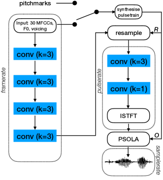
Fig. 1: Overview of the Puffin generator.

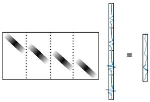
Fig. 2: Overlap add. On the left the $\bm{O}$ matrix.

The following notation is used here: $T$ is number of fixed rate timesteps to be processed by the model; $P$ is the number of glottal pulses in the same example; $F$ is an FFT length which we set to be wider than the largest pulses observed (2048). $T$ is fixed to 512 per example in training and the corresponding $P$ depends on the $F_{0}$ of the speech in the example.

The frame-rate part of the network passes 32 dimensional inputs at 10 ms intervals through 4 simple 1D convolutional layers, each with kernel width $k$ equal to 3, and each followed by leaky ReLU activation. The 32 input features consist of 30 mel frequency cepstral coefficients together with $F_{0}$ (linearly interpolated through unvoiced regions) and voicing. The features are all scaled to appropriate magnitudes using global constants. This results in an array of hidden activations of size T$\times$H. (H=256 for standard setting, and H=1024 for large as explained below.)

As shown in Figure 1, $F_{0}$-related data is used to map between the 3 different rates, using matrix multiplications. Based on an $F_{0}$ track at synthesis time – $F_{0}$ is included among the input features – and on a pitchmark track in training (which specifies the locations of detected glottal closures in the training audio), a resampling matrix $\bm{R}$ and an overlap-add matrix $\bm{O}$ are generated.

Multiplication of fixed rate data with $\bm{R}$ resamples it to the pulse rate by linear interpolation, such that time steps are no longer aligned with fixed rate analysis windows used to provide the input, but instead centered on glottal closure locations. The operation is broadcast across channels, such that channels are interpolated independently of one another. The resampled hidden activations are then processed by a further width-3 convolutional layer followed by leaky ReLU. The final layer with learned parameters is a time-distributed feedforward layer (i.e. a convolutional layer with kernel width 1); its job is to increase the number of channels so that the data can be split into two $F+1$ portions which can be treated as the real and imaginary parts of a pitch-synchronised complex spectrogram. An inverse Fast Fourier Transform (IFFT) is used to convert each slice of this spectrogram into an $F$-dimensional fragment of speech waveform. Following [2, §2.3.3], each of these fragments is treated as a circular buffer whose samples are shifted forward by $F/2$. Although in our system there is no explicit delay compensation step that must be reversed as in [2, §2.2.3], motivation is similar as it is expected that backpropagating through this correction operation will result in intermediate representations of phase that evolve smoothly over time. The fragments are concatenated end-to-end in a PF x 1 dimensional array. $\bm{O}$ is a TS$\times$PF matrix (where S=480, the number of samples in a fixed-rate frame), which is constructed such that the matrix product between it and the concatenated data yields the waveform fragments assembled by overlap-add into a speech waveform of the correct duration. Figure 2 illustrates this operation schematically. The windows are centered on the positions of glottal closures in the output waveform. We use assymetric Hann windows that extend to the two neighbouring glottal closure positions, similar to [2]. There is no strict need to use tapering windows of this kind – in principle rectangular windows are adequate as the waveform fragments that are being assembled are an output of a neural network which can learn to provide data with the appropriate characteristics. However, tests early on in development suggested that using a tapered window is beneficial here.

Note that while implementing resampling and overlap add with matrix multiplication requires the use of matrices covering a sentence or a batch, this is used for the purposes of optimisation only. For deployment these operations are implemented in a way that allows incremental streaming synthesis with minimal lookahead.

$\bm{R}$ and especially $\bm{O}$ are both very large and sparse matrices, and training is only possible using sparse matrix operations. Standard sparse serialisation formats are not adequate to store $\bm{O}$ efficiently but its structure can be exploited to devise an efficient custom format.

2.1 Network training

As with other adversarially trained waveform generators (e.g. [10]), we train the generator using a combination of GAN losses and $L_{1}$ losses. We use a least squares GAN approach as in [10] which is similar in terms of training setup except from the architectures of the discriminators themselves – our discriminators all operate in the frequency domain. They take the time domain signal output by the generator shown in Figure 1, and convert it to a complex spectrogram, whose two channels contain real and imaginary components. Each subdiscriminator contains a stack of five 2D convolutional layers, interspersed with leaky ReLUs and each having a kernel of width 3 along both time and frequency axes (except for the last layer having a kernel size of 1 $\times$ 3). The subdiscriminators therefore have a receptive field covering 9 timesteps and 11 frequency bins. We found it advantageous to use an ensemble of subdiscriminators, covering a number of different analysis window lengths and shifts (in the range 128–4096 points and 256–1024 points, respectively). Furthermore, we saw gains from having such an ensemble specialising in different spectral bands, and assigned 3, 3, and 2 submodels to each of the 3 8kHz frequency bands that make up the 24kHz bandwidth captured by the 48kHz sampling rate.

We also make use of an ensemble of $L_{1}$ losses between natural and generated magnitude spectrograms. As well as a mel spectral loss as used in [10] we found it useful to also use $L_{1}$ losses computed from linear magnitude spectrograms extracted with a variety of 6 different analysis window shifts/length configurations [15, 16].

The contribution of each $L_{1}$ loss was weighted by 0.5 and combined with the adversarial loss terms. In contrast to [10], no feature matching loss was used.

It was found effective to train for a number of steps using only $L_{1}$ losses, which can be done quickly and results in a generator which produces speech that is clear but marred by phase artefacts. Further training using the GAN losses for generator and discriminators reduces these artefacts.

3 Experiments

Table 1: Experimental conditions.

System	Description
N	Natural speech
H1	HiFi-GAN v1 [10]
H3	HiFi-GAN v3 [10]
P	Proposed
PD	Proposed (Downsampled to 22.05kHz)
PL	Proposed (Larger)

3.1 Database

In order to compare our system with a publicly available HiFi-GAN model we use the VCTK dataset [17]. This dataset contains around 20mins of data from 109 native English speakers. The data is available at 96kHz which allows training of 48kHz models.

From the VCTK dataset we held out 9 speakers from training, following the setup of [10] as closely as possible. Exact details of the train/test split used by [10] are not available, but from the demo samples associated with that work we infer the identity of 4 of the nine held-out speakers (p226, p271, p292, p318) excluded from the HiFi-GAN model training. We excluded 5 other speakers (p225, p234, p236, p238, p239) from our training data so that its quantity is comparable to that used to train the existing HiFi-GAN models. To supplement the 4 VCTK evaluation speakers found in this way, we added data from 2 other publicly available single-speaker databases recorded in the same conditions as VCTK [18, 19].

All train and evaluation sentences were endpointed, normalised for loudness [20] and pitchtracked using [21] (minimum and maximum values for $F_{0}$ were set to 50Hz and 400Hz).

3.2 Proposed system

The system described in Section 2 was trained using 2 configurations. The standard configuration P sets number of channels in hidden activations $H$ to 256 and applies block sparsity to the large final layer [11], retaining only 10% of the weights. We also trained a large system with more parameters P^L ($H$=1024) and no sparsity in order to be able to evaluate a Puffin system with comparable complexity to baseline system H³ (see Table 1). Furthermore, Puffin operates at a higher sample rate than the baseline, and to evaluate the contribution of the upper frequency band to perceived quality we downsampled system P’s samples to 22,050Hz and included them as condition P^D.

Training was done with batches of 512 frames of speech concatenated in the time axis. The Adam optimiser was used. We trained both P and P^L for 300,000 steps (c.3.75 hours on a single GTX1080Ti for P) using $L_{1}$ loss terms only; over this interval, desired sparsity was introduced into P using the schedule described in [11]. A further 100,000 steps of training (c.26 hours on the same hardware for P) were carried out for both models, including GAN loss terms, and maintaining the sparsity of system P.

3.3 Baseline systems

We included two versions of HiFi-GAN [10] that differ in terms of the generator’s architecture: H¹ is version 1 (tuned for quality) and H¹ is version 3 (tuned for quality/performance trade-off). Published code and models were used to produce stimuli for these systems.

3.4 Complexity

We compute approximate complexity of each evaluated model by counting the number of operations performed in a forward pass to generate 1 second of speech. This is dominated by the multiplication and addition that must be performed for each weight in the network at the relevant rate. Following [11] we omit computation associated with biases, activation functions, ISTFT etc. – empirically we find that the latter contributes only slightly to overall run time. Calculation of the complexity contribution of each module of each of the 4 systems is given in Table 2.

All modules of all 4 systems are made up of convolutional layers (some transposed, and some used to compute residuals). The essential complexity of a convolutional layer is taken as $iok$ ($i$: number of input channels, $o$: output channels, $k$: kernel width) and is not affected by stride and dilation (see columns 2–4 of Table 2). Residual blocks multiply this by number of convolutional layers used $l$; where sparsity is used, complexity is multiplied by fraction of retained weights $d$ (column 5 of Table 2). This is then multiplied by frequency of operation (column 6) and finally multiplied by 2 (to account for both multiply and add operations). Therefore column 7 of Table 2 shows twice the product of previous columns. Approximate total MFLOPS per system are given after each section.

We note that Puffin’s efficiency depends on the $F_{0}$ of speech to be generated. The pulse rate of 131Hz used in Table 2 is generally representative being the mean value observed in $F_{0}$ tracks extracted from the VCTK training data. However, even under the worst pathological behaviour (all frames voiced and spoken at 400Hz) complexity of system $P$ is still only 322.4 MFLOPS. A desire to limit such variability was part of the motivation to have only a small number of layers operating at the pulse rate in Puffin.

We can see that the proposed vocoder – despite operating at over twice the sampling rate – requires substantially fewer operations per second even when compared to HiFi-GAN version 3 whose smaller generator is intended for wide deployment (188 vs. 3873). Similar comparisons hold with other widely-used systems prioritising efficiency, such as LPCNet [11]. Eq. 8 in [11] (modified to include frame-level terms) gives 2292 MFLOPS with the configuration used there, and 1332 with $N_{A}$ (width of first GRU layer) reduced from 384 to 256. Again, the system we propose is more efficient, despite operating at three times LPCNet’s 16kHz sample rate.

The real time factor of an entire TTS system, incorporating vocoder $P$ as described here as well as acoustic model etc. on a single core of a common choice of hardware for AAC devices (Intel Atom x5-Z8350; RAM: 4GB) is 0.45 to produce speech at 48kHz. A comparable acoustic model combined with LPCNet (even with $N_{A}$ reduced to 256) is not viable on the same machine, where it runs at 1.46 real time to produce 16kHz speech.

Table 2: Complexity of systems evaluated.

$H^{1}$: HiFi-GAN v1
$i$ $o$ $k$ $l$ rate (hz) MFLOPS Conv 80 512 7 - 86 49.3 Upsa 512 256 16 - 86 360.7 Resi 256 256 3 6 689 1625.6 Resi 256 256 7 6 689 3793.0 Resi 256 256 11 6 689 5960.4 Upsa 256 128 16 - 689 722.5 Resi 128 128 3 6 5512 3251.1 Resi 128 128 7 6 5512 7585.9 Resi 128 128 11 6 5512 11920.7 Upsa 128 64 4 - 5512 361.2 Resi 64 64 3 6 11025 1625.7 Resi 64 64 7 6 11025 3793.3 Resi 64 64 11 6 11025 5960.9 Upsa 64 32 4 - 11025 180.6 Resi 32 32 3 6 22050 812.9 Resi 32 32 7 6 22050 1896.7 Resi 32 32 11 6 22050 2980.5 Conv 32 1 7 - 22050 9.9 52890.8

$H^{3}$: HiFi-GAN v3
$i$ $o$ $k$ $l$ rate (hz) MFLOPS Conv 80 256 7 - 86 24.7 Upsa 256 128 16 - 86 90.2 Resi 128 128 3 2 689 135.5 Resi 128 128 5 2 689 225.8 Resi 128 128 7 2 689 316.1 Upsa 128 64 16 - 689 180.6 Resi 64 64 3 2 5512 270.9 Resi 64 64 5 2 5512 451.5 Resi 64 64 7 2 5512 632.2 Upsa 64 32 8 - 5512 180.6 Resi 32 32 3 2 22050 271.0 Resi 32 32 5 2 22050 451.6 Resi 32 32 7 2 22050 632.2 Conv 32 1 7 - 22050 9.9 3872.6

$P$: Puffin standard
$i$ $o$ $k$ $d$ rate (hz) MFLOPS Conv 32 256 3 1.0 100 4.9 Conv 256 256 3 1.0 100 39.3 Conv 256 256 3 1.0 100 39.3 Conv 256 256 3 1.0 100 39.3 Conv 256 256 3 1.0 131 51.5 Conv 256 2064 1 0.1 131 13.8 188.2

$P^{L}$: Puffin large
$i$ $o$ $k$ $d$ rate (hz) MFLOPS Conv 32 1024 3 1.0 100 19.7 Conv 1024 1024 3 1.0 100 629.1 Conv 1024 1024 3 1.0 100 629.1 Conv 1024 1024 3 1.0 100 629.1 Conv 1024 1024 3 1.0 131 824.2 Conv 1024 2064 1 1.0 131 553.7 3285.0

3.5 Listening experiment design

We performed a MUSHRA-style listening test where participants were asked to rate the quality of the generated samples. In total we generated 9 sentences per speaker in the test set (in total 54 sentences); all sentences contained different text. Sentences were randomly selected from the set each speaker recorded. The sentences were then divided equally across 3 different listening test, such that each test contained 18 number of sentences per speaker. Each participant was randomly assigned to a specific test; i.e. each participant was presented with 18 number of MUSHRA screens/sentences. The test duration was around 20mins.

Participants were recruited via Prolific Academic using the following screening criteria: between 18 and 50 years old, no known hearing impairement or difficulties, and English as a first language. Participants were asked to perform the test in a quiet place wearing headphones. 20 participants took part in the study.

3.6 Results

Figure 3 shows the results of the listening test in the form of a boxplot. Orange lines indicate the mean rating for each system. To compute significance, a Wilcoxon signed-rank test was used (significance level = 0.05), with a Bonferroni correction for multiple pairwise comparisons. Following the standard exclusion criteria in [22], participants were discarded if they rated the hidden natural reference less than 90 more than 15% of times, which resulted in 14 valid participants (out of 20). A significant difference between the ratings for H³ and all other systems was found, as well as for N and all other systems; H¹ was significantly different from all systems except P^D (indicated by blue dots). For the various proposed systems, P was not rated significantly different from the rest (indicated by yellow dots), while P^D and P^L were significantly different from each other.

The higher rating of system P (the proposed system at 48kHz) than that of system P^D (the proposed system downsampled to 22kHz) justifies the generation of fullband speech. System H¹ (the strong benchmark) is not significantly different from the downsampled proposed system. We suggest that this inconsistency in ratings of speech at difference sample rates requires more evaluation, potentially looking at whether people consistently rate natural speech at these two sampling rates as different.

The ratings of P and P^L are similar. This indicates that the extra complexity of P^L is not required, although some benefit is suggested.

Finally, H³ is rated as significantly worse than all other systems. Informal listening of samples generated by this system suggests that this model suffers from some periodicity/voicing artefacts, which are not present in the other systems.

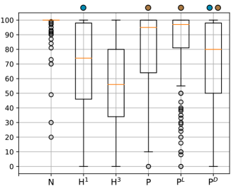
Fig. 3: Boxplot of listening test scores.

4 Conclusions

In this work we have presented a new waveform generation method combining traditional signal processing methods from an older generation of vocoders with new deep learning approaches. Our results, firstly, suggest that it is worth pursuing fullband speech, despite the current focus on e.g. 22kHz audio in neural vocoder research. More importantly, we have found that our system is able to generate speech whose quality matches that of strong baseline systems, at a fraction of the run time computational cost. This makes the deployment of high quality TTS voices on low-powered devices (such that are often used by people with AAC needs) feasible, meaning a population of users whose communication might be solely carried out using TTS could also benefit from recent quality improvements.

References

- [1] Masanori Morise, Fumiya Yokomori, and Kenji Ozawa, “WORLD: A Vocoder-Based High-Quality Speech Synthesis System for Real-Time Applications,” IEICE Trans. Inf. Syst., vol. E99.D, no. 7, 2016.
- [2] Felipe Espic, Cassia Valentini-Botinhao, and Simon King, “Direct modelling of magnitude and phase spectra for statistical parametric speech synthesis,” in Proc. Interspeech, 2017, pp. 1383–1387.
- [3] Soroush Mehri, Kundan Kumar, Ishaan Gulrajani, Rithesh Kumar, Shubham Jain, Jose Sotelo, Aaron Courville, and Yoshua Bengio, “SampleRNN: An unconditional end-to-end neural audio generation model,” in Proc. ICLR, 2017.
- [4] Jonathan Shen, Ruoming Pang, Ron J. Weiss, Mike Schuster, Navdeep Jaitly, Zongheng Yang, Zhifeng Chen, Yu Zhang, Yuxuan Wang, RJ Skerry Ryan, Rif A. Saurous, Yannis Agiomyrgiannakis, and Yonghui Wu, “Natural TTS synthesis by conditioning Wavenet on MEL spectrogram predictions,” in Proc. ICASSP, 2018, pp. 4779 – 4783.
- [5] Keisuke Matsubara, Takuma Okamoto, Ryoichi Takashima, Tetsuya Takiguchi, Tomoki Toda, and Hisashi Kawai, “Comparison of real-time multi-speaker neural vocoders on CPUs,” Acoustical Science and Technology, vol. 43, no. 2, pp. 121–124, 2022.
- [6] Aäron van den Oord, Sander Dieleman, Heiga Zen, Karen Simonyan, Oriol Vinyals, Alexander Graves, Nal Kalchbrenner, Andrew Senior, and Koray Kavukcuoglu, “WaveNet: A generative model for raw audio,” https://arxiv.org/abs/1609.03499, 2016, arXiv:1609.03499.
- [7] Aäron van den Oord, Yazhe Li, Igor Babuschkin, Karen Simonyan, Oriol Vinyals, Koray Kavukcuoglu, George van den Driessche, Edward Lockhart, Luis Cobo, Florian Stimberg, Norman Casagrande, Dominik Grewe, Seb Noury, Sander Dieleman, Erich Elsen, Nal Kalchbrenner, Heiga Zen, Alex Graves, Helen King, Tom Walters, Dan Belov, and Demis Hassabis, “Parallel WaveNet: Fast high-fidelity speech synthesis,” in Proc. ICML, Jul 2018, pp. 3918–3926.
- [8] Ryan Prenger, Rafael Valle, and Bryan Catanzaro, “Waveglow: A flow-based generative network for speech synthesis,” in Proc. ICASSP, 2019, pp. 3617–3621.
- [9] Kundan Kumar, Rithesh Kumar, Thibault de Boissiere, Lucas Gestin, Wei Zhen Teoh, Jose Sotelo, Alexandre de Brebisson, Yoshua Bengio, and Aaron Courville, “MelGAN: Generative adversarial networks for conditional waveform synthesis,” http://arxiv.org/abs/1910.06711, 2019, arXiv:1910.06711.
- [10] Jungil Kong, Jaehyeon Kim, and Jaekyoung Bae, “HiFi-GAN: Generative adversarial networks for efficient and high fidelity speech synthesis,” in Proc. NeurIPS, 2020, vol. 33, pp. 17022–17033.
- [11] Jean-Marc Valin and Jan Skoglund, “LPCNET: improving neural speech synthesis through linear prediction,” in Proc. ICASSP, 2019, pp. 5891–5895.
- [12] Yang Cui, Xi Wang, Lei He, and Frank K. Soong, “An efficient subband linear prediction for LPCNet-based neural synthesis,” in Proc. Interspeech, 2020, pp. 3555–3559.
- [13] Takuhiro Kaneko, Kou Tanaka, Hirokazu Kameoka, and Shogo Seki, “ISTFTNET: Fast and Lightweight Mel-Spectrogram Vocoder Incorporating Inverse Short-Time Fourier Transform,” in Proc. ICASSP, 2022, pp. 6207–6211.
- [14] Jacob J Webber, Cassia Valentini-Botinhao, Evelyn Williams, Gustav Eje Henter, and Simon King, “Autovocoder: Fast waveform generation from a learned speech representation using differentiable digital signal processing,” in Proc. ICASSP, 2023.
- [15] Xin Wang, Shinji Takaki, and Junichi Yamagishi, “Neural source-filter waveform models for statistical parametric speech synthesis,” IEEE/ACM Trans. Audio, Speech and Lang. Proc., vol. 28, pp. 402–415, 2020.
- [16] Ryuichi Yamamoto, Eunwoo Song, and Jae-Min Kim, “Parallel wavegan: A fast waveform generation model based on generative adversarial networks with multi-resolution spectrogram,” in Proc. ICASSP, 2020, pp. 6199–6203.
- [17] Junichi Yamagishi, Christophe Veaux, and Kirsten MacDonald, “CSTR VCTK corpus: English multi-speaker corpus for CSTR voice cloning toolkit,” https://doi.org/10.7488/ds/1994, 2017.
- [18] Cassia Valentini-Botinhao, Catherine Mayo, and Martin Cooke, “Hurricane natural speech corpus - higher quality version,” https://doi.org/10.7488/ds/2482, 2019.
- [19] Cassia Valentini-Botinhao and Junichi Yamagishi, “Alba speech corpus,” https://doi.org/10.7488/ds/2506, 2019.
- [20] International Telecommunication Union Radiocommunication Assembly, International Telecommunication Union, Recommendation G.191: Software Tools and Audio Coding Standardization,, November 2005.
- [21] “REAPER: Robust Epoch And Pitch EstimatoR,” https://github.com/google/REAPER, 2017.
- [22] International Telecommunication Union Radiocommunication Assembly, Geneva, Switzerland, Method for the subjective assessment of intermediate quality level of coding systems, March 2003.