Resonance $X(3960)$ as a hidden charm-strange scalar tetraquark

Abstract

We investigate features of the hidden charm-strange scalar tetraquark $c\overline{c}s\overline{s}$ by calculating its spectral parameters and width, and we compare the obtained results with the mass and width of the resonance $X(3960)$ discovered recently in the LHCb experiment. We model the tetraquark as a diquark-antidiquark state $X=[cs][\overline{c}\overline{s}]$ with spin-parities $J^{\mathrm{PC}}=0^{++}$. The mass and current coupling of $X$ are calculated using the QCD two-point sum rules by taking into account various vacuum condensates up to dimension $10$. The width of the tetraquark $X$ is estimated via the decay channels $X\to D_{s}^{+}D_{s}^{-}$ and $X\to\eta_{c}\eta^{(\prime)}$. The partial widths of these processes are expressed in terms of couplings $G$, $g_{1}$ and $g_{2}$ which describe the strong interactions of particles at the vertices $XD_{s}^{+}D_{s}^{-}$, $X\eta_{c}\eta^{\prime}$ and $X\eta_{c}\eta$, respectively. Numerical values of $G$, $g_{1}$ and $g_{2}$ are evaluated by employing the three-point sum rule method. Comparing the results $m=(3976\pm 85)~{}\mathrm{MeV}$ and $\Gamma_{\mathrm{X}}=(42.2\pm 12.0)~{}\mathrm{MeV}$ obtained for parameters of the tetraquark $X$ and experimental data of the LHCb Collaboration, we conclude that the resonance $X(3960)$ can be considered as a candidate to a scalar diquark-antidiquark state.

I Introduction

Recently, the LHCb Collaboration reported the observation of a new threshold peaking structure $X(3960)$ in the $D_{s}^{+}D_{s}^{-}$ invariant mass distribution in the $B^{+}\rightarrow D_{s}^{+}D_{s}^{-}K^{+}$ decay LHCb:2022vsv . Performed analysis demonstrated that it is a scalar resonance $J^{\mathrm{PC}}=0^{++}$ with the mass and width

$$m_{\mathrm{exp}} = 3956\pm 5\pm 10~{}\mathrm{MeV},$$

$$\Gamma_{\mathrm{exp}} = 43\pm 13\pm 8~{}\mathrm{MeV}.$$ (1)

The collaboration also found an additional structure around $4140\ \mathrm{MeV}$ with spin-parities $0^{++}$. The resonance $X(3960)$ was interpreted by LHCb as a four-quark state with the content $c\overline{c}s\overline{s}$, whereas the structure $4140~{}\mathrm{MeV}$ may be either a new resonance or $J/\psi\phi\leftrightarrow D_{s}^{+}D_{s}^{-}$ coupled-channel effect.

Four-quark exotic mesons composed of quarks $c\overline{c}s\overline{s}$ with different quantum numbers are not something new for both experimental and theoretical physicists. In fact, resonances with the quark content $c\overline{c}s\overline{s}$ were fixed by LHCb in the $J/\psi\phi$ invariant mass distribution in the process $B^{+}\rightarrow J/\psi\phi K^{+}$ Aaij:2016iza . The discovered states $X(4140)$ and $X(4274)$ are axial-vector particles with $J^{\mathrm{PC}}=1^{++}$, whereas the spin-parities of $X(4500)$ and $X(4700)$ are $J^{\mathrm{PC}}=0^{++}$. It should be noted that resonances $X(4140)$ and $X(4274)$ were previously seen by the CDF Collaboration Aaltonen:2009tz in the decays $B^{\pm}\rightarrow J/\psi\phi K^{\pm}$, and confirmed later by CMS Chatrchyan:2013dma and D0 experiments Abazov:2013xda . The scalar structures $X(4500)$ and $X(4700)$ were fixed by the LHCb Collaboration for the first time.

In experiments numerous exotic vector mesons built of $c\overline{c}s\overline{s}$ quarks were observed as well. Thus, the state $Y(4660)$ was found for the first time by the Belle Collaboration in the process $e^{+}e^{-}\rightarrow\gamma_{\mathrm{ISR}}\psi(2S)$ $\pi^{+}\pi^{-}$ as one of two resonant structures in the $\psi(2S)\pi^{+}\pi^{-}$ invariant mass distribution. Because $Y(4660)$ was produced in the $e^{+}e^{-}$ annihilation its quantum numbers are $J^{\mathrm{PC}}=1^{--}$. The structure $X(4630)$ was discovered by LHCb in the $J/\psi\phi$ invariant mass distribution of the decay $B^{+}\rightarrow J/\psi\phi K^{+}$ LHCb:2021uow .

Theoretical studies of four-quark states $c\overline{c}s\overline{s}$ have also rich history. The charmoniumlike exotic mesons with $s\overline{s}$ component were investigated by means of different methods in numerous publications (see, as examples, Refs. Nieves:2012tt ; Wang:2013exa ; Lebed:2016yvr ; Chen:2017dpy ; Meng:2020cbk ). Comprehensive analyses of some of hidden-charm diquark-antidiquark systems $[cs][\overline{c}\overline{s}]$ were carried out in our articles as well. Thus, the axial-vector resonances $X(4140)$ and $X(4274)$ were investigated in Ref. Agaev:2017foq , in which, we treated them as diquark-antidiquark states built of scalar and axial-vector components belonging to triplet and sextet representations of $SU_{c}(3)$ color group, respectively. We calculated not only their masses and current couplings (or pole residues) but also evaluated full widths of these tetraquarks. Predictions for parameters of  the color-triplet diquark-antidiquark state allowed us to interpret it as the resonance $X(4140)$. Contrary, the full width of the tetraquark with color sextet ingredients is considerably wider than that of the resonance $X(4274)$. Therefore, to explain the internal organization of $X(4274)$ alternative models should be examined, though existence of a new axial-vector resonance with the mass $m\approx 4274~{}\mathrm{MeV}$ and full width $\Gamma\approx 200~{}\mathrm{MeV}$ cannot be excluded.

The vector resonance $Y(4660)$ was studied as a diquark-antidiquark vector state $[cs][\overline{c}\overline{s}]$ with $J^{\mathrm{PC}}=1^{--}$ in our work Sundu:2018toi . Results obtained there for the mass and full width of this structure made it possible to interpret the resonance $Y(4660)$ as the diquark-antidiquark exotic meson. The detailed analysis of $X(4630)$ was performed in Ref. Agaev:2022iha by assuming that it is a vector tetraquark $[cs][\overline{c}\overline{s}]$ with spin-parities $J^{\mathrm{PC}}=1^{-+}$. Here, a nice agreement was obtained between the LHCb data for parameters of the resonance $X(4630)$ and theoretical predictions of the diquark-antidiquark model. There are numerous articles devoted to experimental studies and theoretical analysis of hidden charm-strange four-quark mesons in the literature: Relatively full list of such publications can be found in Refs. LHCb:2022vsv ; Agaev:2017foq ; Sundu:2018toi ; Agaev:2022iha .

First announcement made in Ref. X3960 about discovery of the resonance $X(3960)$ triggered extreme interest to this state. In papers Bayar:2022dqa ; Ji:2022uie ; Xin:2022bzt ; Xie:2022lyw ; Chen:2022dad ; Guo:2022ggl ; Guo:2022crh appeared afterwards, authors addressed different aspects of its internal organization, production mechanisms and rates, placed $X(3960)$ into various four-quark multiplets. The coupled-channel explanation of $X(3960)$ was suggested in Ref. Bayar:2022dqa , where it emerges as an enhancement in the $D_{s}^{+}D_{s}^{-}$ mass distribution via interaction of the $D^{+}D^{-}$ and $D_{s}^{+}D_{s}^{-}$ coupled-channels. In Ref. Xin:2022bzt the authors assigned $X(3960)$ the hadronic molecule $D_{s}^{+}D_{s}^{-}$, and performed studies in the context of the sum rule method. The resonance $X(3960)$ was explained also as near the $D_{s}^{+}D_{s}^{-}$ threshold enhancement due to the contribution of the conventional $P$-wave charmonium $\chi_{c0}(2P)$ Guo:2022ggl .

In the present article, we explore the tetraquark $X=[cs][\overline{c}\overline{s}]$ with spin-parities $J^{\mathrm{PC}}=0^{++}$ and compute its parameters. The mass and current coupling of $X$ are evaluated using the QCD two-point sum rule method. Its full width is estimated using the decay channels $X\rightarrow D_{s}^{+}D_{s}^{-}$ and $X\rightarrow\eta_{c}\eta^{(\prime)}$. Partial widths of these processes are expressed through strong couplings $G$, $g_{1}$ and $g_{2}$ of particles at the vertices $XD_{s}^{+}D_{s}^{-}$, $X\eta_{c}\eta^{\prime}$, and $X\eta_{c}\eta$, respectively. To calculate $G$, $g_{1}$ and $g_{2}$, we employ technical tools of the three-point sum rule approach. Results found for parameters of the state $X$ are confronted with the LHCb data to verify the diquark-antidiquark model for $X(3960)$.

This paper is organized in the following way: In Sec. II, we compute the mass and current coupling of the tetraquark $X$ by means of the QCD two-point sum rule method. The decay $X\rightarrow D_{s}^{+}D_{s}^{-}$ is studied in Sec. III, where we calculate the coupling $G$ and partial width of this process. The strong couplings $g_{1}$ and $g_{2}$ and partial widths of the decays $X\rightarrow\eta_{c}\eta^{\prime}$ and $X\rightarrow\eta_{c}\eta$, as well as the full width of $X$ are found in Sec. IV. The section V is reserved for our concluding notes.

II Mass and current coupling of the tetraquark $X$

In this section, we consider the scalar diquark-antidiquark state $X=[cs][\overline{c}\overline{s}]$ and extract its spectroscopic parameters from the two-point sum rule analysis Shifman:1978bx ; Shifman:1978by . It is known that the sum rule method operates with correlation functions and interpolating currents of particles under investigations. There are different ways to construct a scalar tetraquark and corresponding current using a diquark and an antidiquark with different spin-parities Chen:2010ze . Thus, one may construct such state using the pseudoscalar $c^{T}Cs$ or vector $c^{T}C\gamma_{\mu}\gamma_{5}s$ diquarks and corresponding antidiquarks, where $C$ is the charge-conjugation operator. But, we assume that $X$ is built of a scalar diquark $c^{T}C\gamma_{5}s$ and antidiquark $\overline{c}\gamma_{5}C\overline{s}^{T}$: The reason is that the scalar diquark (antidiquark) configuration is the most attractive and stable two-quark system Jaffe:2004ph .

The structures $\epsilon c^{T}C\gamma_{5}s$ and $\widetilde{\epsilon}\overline{c}\gamma_{5}C\overline{s}^{T}$ are the color antitriplet and triplet states of the color $SU_{c}(3)$ group, respectively. Then the interpolating current for the tetraquark $X$ has the form

$$J(x)=\epsilon\widetilde{\epsilon}\left[c_{b}^{T}(x)C\gamma_{5}s_{c}(x)\right]\left[\overline{c}_{m}(x)\gamma_{5}C\overline{s}_{n}^{T}(x)\right],$$ (2)

where $\epsilon\widetilde{\epsilon}=\epsilon^{abc}\epsilon^{amn}$ and $a,b,c,m$ and $n$ are color indices. This current belongs to $[\overline{\mathbf{3}}_{c}]_{cs}\otimes[\mathbf{3}_{c}]_{\overline{c}\overline{s}}$ representation of the color group and corresponds to the scalar state with quantum numbers $J^{\mathrm{PC}}=0^{++}$. The current $J(x)$ describes a ground-state scalar particle with lowest mass and required spin-parities.

The mass $m$ and coupling $f$ of the tetraquark $X$ can be determined from analysis of the correlation function $\Pi(p)$

$$\Pi(p)=i\int d^{4}xe^{ipx}\langle 0|\mathcal{T}\{J(x)J^{{\dagger}}(0)\}|0\rangle.$$ (3)

To derive the required sum rules, one has to express $\Pi(p)$ using the spectroscopic parameters of the tetraquark $X$. For these purposes, we insert into the correlation function $\Pi(p)$ a complete set of states with quantum numbers $0^{++}$ and perform integration over $x$ in Eq. (3). As a result, we get

$$\Pi^{\mathrm{Phys}}(p)=\frac{\langle 0|J|X(p\rangle\langle X(p)|J^{\dagger}|0\rangle}{m^{2}-p^{2}}+\cdots.$$ (4)

The obtained expression forms a hadronic representation of $\Pi(p)$ and is the phenomenological (physical) side of sum rule. Here, the contribution coming from the ground-state particle $X$ is written down explicitly, whereas contributions of higher resonances and continuum states are denoted by the ellipses.

The function $\Pi^{\mathrm{Phys}}(p)$ can be further simplified by employing the matrix element

$$\langle 0|J|X(p)\rangle=fm.$$ (5)

It is easy to find that, in terms of the parameters $m$ and $f$, the function $\Pi^{\mathrm{Phys}}(p)$ takes the following form

$$\Pi^{\mathrm{Phys}}(p)=\frac{m^{2}f^{2}}{m^{2}-p^{2}}+\cdots.$$ (6)

The $\Pi^{\mathrm{Phys}}(p)$ has simple Lorentz structure proportional to $\mathrm{I}$, and relevant invariant amplitude $\Pi^{\mathrm{Phys}}(p^{2})$ is given by r.h.s. of Eq. (6).

To determine the QCD side of the sum rules $\Pi^{\mathrm{OPE}}(p)$, we use the interpolating current $J(x)$ in Eq. (3), and contract the heavy and light quark fields. After simple manipulations, we obtain

$$\Pi^{\mathrm{OPE}}(p)=i\int d^{4}xe^{ipx}\epsilon\widetilde{\epsilon}\epsilon^{\prime}\widetilde{\epsilon}^{\prime}\mathrm{Tr}\left[\gamma_{5}\widetilde{S}_{c}^{bb^{\prime}}(x)\right.$$

$$\left.\times\gamma_{5}S_{s}^{cc^{\prime}}(x)\right]\mathrm{Tr}\left[\gamma_{5}\widetilde{S}_{s}^{n^{\prime}n}(-x)\gamma_{5}S_{c}^{m^{\prime}m}(-x)\right],$$ (7)

where $S_{c}(x)$ and $S_{s}(x)$ are the $c$ and $s$-quark propagators, respectively. Explicit expressions of these propagators are presented in the Appendix (see, also Ref. Agaev:2020zad ). In Eq. (7), we have also used the notation

$$\widetilde{S}_{c(s)}(x)=CS_{c(s)}^{T}(x)C.$$ (8)

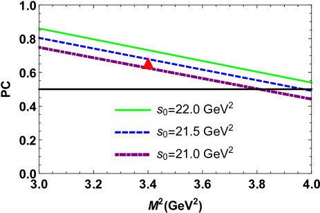
Figure 1: Pole contribution as a function of the Borel parameter $M^{2}$ at various $s_{0}$. The horizontal black line limits a region $\mathrm{PC}=0.5$. The red triangle fixes the point, where the mass $m$ of the tetraquark $X$ has effectively been extracted.

The correlation function $\Pi^{\mathrm{OPE}}(p)$ should be computed in the operator product expansion ($\mathrm{OPE}$) with some accuracy. The $\Pi^{\mathrm{OPE}}(p)$ has also a trivial structure $\sim\mathrm{I}$ and is characterized by an amplitude $\Pi^{\mathrm{OPE}}(p^{2})$. Having equated the invariant amplitudes $\Pi^{\mathrm{Phys}}(p^{2})$ and $\Pi^{\mathrm{OPE}}(p^{2})$, one gets the master QCD sum rule equality. Afterwards, one needs to suppress contributions of higher resonances and continuum states by applying the Borel transformation. The assumption about quark-hadron duality allows one to subtract these suppressed terms from the obtained expression. After these operations, the sum rule equality starts to depend on the Borel $M^{2}$ and continuum threshold $s_{0}$ parameters.

The Borel transformation of $\Pi^{\mathrm{Phys}}(p^{2})$ is a simple function, whereas for $\Pi^{\mathrm{OPE}}(p^{2})$ we get a complicated formula

$$\Pi(M^{2},s_{0})=\int_{4\mathcal{M}^{2}}^{s_{0}}ds\rho^{\mathrm{OPE}}(s)e^{-s/M^{2}}+\Pi(M^{2}),$$ (9)

where $\mathcal{M}=m_{c}+m_{s}$. In numerical computations we set $m_{s}^{2}=0$, but include into analysis terms proportional to $m_{s}$. The two-point spectral density $\rho^{\mathrm{OPE}}(s)$ is calculated as an imaginary part of the correlation function. The second term $\Pi(M^{2})$ includes nonperturbative contributions extracted directly from $\Pi^{\mathrm{OPE}}(p)$. The correlator $\Pi(M^{2},s_{0})$ is computed by taking into account nonperturbative terms up to dimension $10$. Explicit expression of $\Pi(M^{2},s_{0})$ is written down in the Appendix.

The sum rules for $m$ and $f$ are expressed via the invariant amplitude $\Pi(M^{2},s_{0})$,

$$m^{2}=\frac{\Pi^{\prime}(M^{2},s_{0})}{\Pi(M^{2},s_{0})},$$ (10)

and

$$f^{2}=\frac{e^{m^{2}/M^{2}}}{m^{2}}\Pi(M^{2},s_{0}),$$ (11)

where $\Pi^{\prime}(M^{2},s_{0})=d\Pi(M^{2},s_{0})/d(-1/M^{2})$.

To carry out the numerical computations in accordance with Eqs. (10) and (11), we have to fix values of different vacuum condensates. The reason is that the sum rules for $m^{2}$ and $f^{2}$ through $\Pi(M^{2},s_{0})$ depend on the vacuum expectation values of quark, gluon and mixed operators. The vacuum condensates, that enter to the sum rules Eqs. (10) and (11), are universal quantities obtained from analysis of various hadronic processes Shifman:1978bx ; Shifman:1978by ; Ioffe:1981kw ; Ioffe:2005ym ; Narison:2015nxh

$$\langle\overline{q}q\rangle=-(0.24\pm 0.01)^{3}~{}\mathrm{GeV}^{3},\ \langle\overline{s}s\rangle=(0.8\pm 0.1)\langle\overline{q}q\rangle,$$

$$\langle\overline{s}g_{s}\sigma Gs\rangle=m_{0}^{2}\langle\overline{s}s\rangle,\ m_{0}^{2}=(0.8\pm 0.1)~{}\mathrm{GeV}^{2},\$$

$$\langle\frac{\alpha_{s}G^{2}}{\pi}\rangle=(0.012\pm 0.004)~{}\mathrm{GeV}^{4},$$

$$\langle g_{s}^{3}G^{3}\rangle=(0.57\pm 0.29)~{}\mathrm{GeV}^{6},$$

$$m_{c}=(1.27\pm 0.02)~{}\mathrm{GeV},\ \ \ m_{s}=93_{-5}^{+11}~{}\mathrm{MeV}.$$ (12)

It is seen that the vacuum condensate of the strange quark differs from the $\langle 0|\overline{q}q|0\rangle$ Ioffe:1981kw . The mixed condensates $\langle\overline{q}g_{s}\sigma Gq\rangle$ and $\langle\overline{s}g_{s}\sigma Gs\rangle$ are expressed in terms of the corresponding quark condensates and the parameter $m_{0}^{2}$. The numerical value of the latter was extracted from analysis of baryonic resonances in Ref. Ioffe:2005ym . For the gluon condensate $\langle g^{3}G^{3}\rangle$, we use the estimate given in Ref. Narison:2015nxh . This list also contains the masses of $c$ and $s$ quarks in the $\overline{\mathrm{MS}}$-scheme from Ref. PDG:2022 .

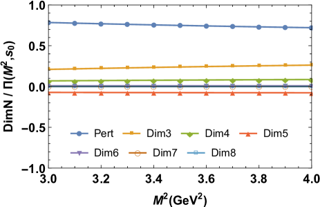
Figure 2: Different contributions to $\Pi(M^{2},s_{0})$ normalized to $1$ as functions of the Borel parameter $M^{2}$. All lines in this figure have been calculated at $s_{0}=21.5~{}\mathrm{GeV}^{2}$.

Predictions for $m$ and $f$ extracted from the sum rules depend also on the Borel and continuum subtraction parameters $M^{2}$ and $s_{0}$. In general, physical quantities should not contain residual effects connected with the choice of $M^{2}$. But in a real situation $m$ and $f$  bear imprints of operations fulfilled to isolate contribution of the ground-state particle to sum rules. A way to solve this problem is using some prescriptions to minimize the unwanted effects. To this end, in the sum rule analysis, the choice of a working window for the Borel parameter $M^{2}$ is restricted by the dominance of the pole contribution ($\mathrm{PC}$) and convergence of $\mathrm{OPE}$. To quantify these constraints, it is convenient to introduce the expressions

$$\mathrm{PC}=\frac{\Pi(M^{2},s_{0})}{\Pi(M^{2},\infty)},$$ (13)

and

$$R(M^{2})=\frac{\Pi^{\mathrm{DimN}}(M^{2},s_{0})}{\Pi(M^{2},s_{0})}.$$ (14)

First of them is a measure of the pole contribution and necessary to find the higher border of the $M^{2}$ region. In Eq. (14) $\Pi^{\mathrm{DimN}}(M^{2},s_{0})$ indicates the last three terms in $\mathrm{OPE}$ of $\Pi(M^{2},s_{0})$, i.e., $\mathrm{DimN=Dim(8+9+10)}$. We use $R(M^{2})$ to estimate the convergence of $\mathrm{OPE}$ and fix a lower limit of $M^{2}$.

In working regions of $M^{2}$ and $s_{0}$ the perturbative contribution to the correlation function $\Pi(M^{2},s_{0})$ has to be larger than the ones due to nonperturbative terms. Besides, the window for $M^{2}$ should generate stable predictions for the extracted physical quantities. Performed analysis demonstrates that windows for $M^{2}$ and $s_{0}$, which satisfy these constraints, are

$$M^{2}\in[3,4]~{}\mathrm{GeV}^{2},\ s_{0}\in[21,22]~{}\mathrm{GeV}^{2}.$$ (15)

Indeed, in the regions Eq. (15) the pole contribution varies on average within the interval

$$0.80\geq\mathrm{PC}\geq 0.49.$$ (16)

In Fig. 1, the $\mathrm{PC}$ is drawn as a function of the Borel parameter at various $s_{0}$. It is seen that except for a small domain $M^{2}>2.8~{}\mathrm{GeV}^{2}$ at $s_{0}=21~{}\mathrm{GeV}^{2}$ the dominance of the pole contribution, i.e., the constraint $\mathrm{PC}\geq 0.5$ is fulfilled for all values of the parameters $M^{2}$ and $s_{0}$.

In Fig. 2, we demonstrate the dependence on $M^{2}$ of the perturbative and different nonperturbative contributions to $\Pi(M^{2},s_{0})$. It is evident that the perturbative term is considerably larger than the nonperturbative contributions, and constitutes $80\%$ of $\Pi(M^{2},s_{0})$ at $M^{2}=3~{}\mathrm{GeV}^{2}$. This figure confirms also convergence of the $\mathrm{OPE}$, which implies that the contributions of the nonperturbative terms reduce by increasing the dimensions of the corresponding operators. The $\mathrm{Dim3}$ term numerically exceeds the contributions of other nonperturbative operators, whereas $\mathrm{Dim9}$ and $\mathrm{Dim10}$ terms are very small and not shown in the plot. The quantity $R(M^{2})$ at $M^{2}=3~{}\mathrm{GeV}^{2}$ is less than $0.01$, which proves numerically the convergence of the $\mathrm{OPE}$ and correctness of the lower value of $M^{2}$.

The residual dependences of the mass $m$ of the tetraquark $X$ on the Borel and continuum subtraction parameters $M^{2}$ and $s_{0}$ are shown in Fig. 3. It is seen that the window for $M^{2}$, where parameters of $X$ are extracted, leads to approximately stable predictions for $m$. At the same time, one observes some variations of $m$ against the Borel parameter $M^{2}$. This effect allows us to estimate the uncertainties of the sum rule predictions. Variation of the continuum threshold parameter $s_{0}$ is another source of the theoretical ambiguities. The region for $s_{0}$ has to meet the constraints coming from the dominance of $\mathrm{PC}$ and convergence of the $\mathrm{OPE}$. The parameter $\sqrt{s_{0}}$ bears also information on the mass $m^{\ast}$ of the first radial excitation of the tetraquark $X$, and should obey $\sqrt{s_{0}}\leq m^{\ast}$.

The results for the mass $m$ and coupling $f$ are evaluated as mean values of these quantities calculated in the working regions (15):

$$m = (3976\pm 85)~{}\mathrm{MeV},$$

$$f = (7.3\pm 0.8)\times 10^{-3}~{}\mathrm{GeV}^{4}.$$ (17)

The mass and coupling written down in Eq. (17) effectively correspond to the sum rule predictions at $M^{2}=3.4~{}\mathrm{GeV}^{2}$ and $s_{0}=21.5~{}\mathrm{GeV}^{2}$ shown in Fig. 1 by the red triangle. This point is located approximately at the middle of the working regions, where the pole contribution is $\mathrm{PC}\approx 0.64$. This fact and other details discussed above guarantees the ground-state nature of $X$ and credibility of the final results. An estimate for the mass of the excited tetraquark $m^{\ast}\geq(m+650)~{}\mathrm{MeV}$ stemming from Eqs. (15) and (17) is also reasonable for the double-heavy tetraquarks.

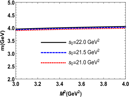
Figure 3: Mass $m$ of the tetraquark $X$ as a function of the Borel $M^{2}$ (left), and the continuum threshold $s_{0}$ parameters (right)

.

III Decay $X\rightarrow D_{s}^{+}D_{s}^{-}$

The spectroscopic parameters of the tetraquark $X$ form a basis to determine its kinematically allowed decay channels. Because $X(3960)$ was observed in the $D_{s}^{+}D_{s}^{-}$ invariant mass distribution, we treat the decay $X\rightarrow D_{s}^{+}D_{s}^{-}$ as a dominant mode of $X$. The two-meson threshold for this process $\approx 3937~{}\mathrm{MeV}$ is below the mass of $X$. Other decay channels that should be considered in this paper are $X\rightarrow\eta_{c}\eta^{\prime}$ and $X\rightarrow\eta_{c}\eta$. The kinematical limits for realization of these processes do not exceed $\approx 3941~{}\mathrm{MeV}$ which is less than $m$ as well. It is easy to see also that decays of the scalar tetraquark with spin-parities $J^{\mathrm{PC}}=0^{++}$ to two pseudoscalar mesons with $J^{\mathrm{PC}}=0^{-+}$ preserves the spin and quantum numbers $\mathrm{P}$ and $\mathrm{C}$ of the initial state $X$.

The partial width of the decay $X\rightarrow D_{s}^{+}D_{s}^{-}$ is determined by a coupling $G$ that describes the strong interaction at the vertex $XD_{s}^{+}D_{s}^{-}$. Apart from $G$, it depends also on the masses and decay constants of the initial and final particles. The mass and coupling of $X$ have been calculated in the present article, whereas physical parameters of the mesons $D_{s}^{+}$ and $D_{s}^{-}$ are known from other sources. Therefore, the only physical quantity to be found here is the strong coupling $G$.

To evaluate $G$, we use the QCD three-point sum rule method, and start our analysis from the correlation function

$$\Pi(p,p^{\prime})=i^{2}\int d^{4}xd^{4}ye^{i(p^{\prime}y-px)}\langle 0|\mathcal{T}\{J^{D_{s}^{+}}(y)$$

$$\times J^{D_{s}^{-}}(0)J^{\dagger}(x)\}|0\rangle,$$ (18)

where $J(x)$,$\ J^{D_{s}^{+}}(y)$ and $J^{D_{s}^{-}}(0)$ are the interpolating currents for the tetraquark $X$, and the pseudoscalar mesons $D_{s}^{+}$ and $D_{s}^{-}$, respectively. The four-momenta of $X$ and $D_{s}^{+}$ are denoted by $p$ and $p^{\prime}$, whereas the momentum of the meson $D_{s}^{-}$ is equal to $q=p-p^{\prime}$. The current $J(x)$ is given by Eq. (2), whereas for the mesons, we use the following currents:

$$\ J^{D_{s}^{+}}(x) = \overline{s}_{j}(x)i\gamma_{5}c_{j}(x),$$

$$J^{D_{s}^{-}}(x) = \overline{c}_{i}(x)i\gamma_{5}s_{i}(x),$$ (19)

with $i$ and $j$ being the color indices.

To continue our study of the strong coupling $G$, we follow usual recipes of the sum rule method and compute the correlation function $\Pi(p,p^{\prime})$. To this end, we employ the physical parameters of the tetraquark and mesons participating in this process. The correlator $\Pi(p,p^{\prime})$ found by this way constitutes the phenomenological side $\Pi^{\mathrm{Phys}}(p,p^{\prime})$ of the sum rule. It is not difficult to see that

$$\Pi^{\mathrm{Phys}}(p,p^{\prime})=\frac{\langle 0|J^{D_{s}^{+}}|D_{s}^{+}(p^{\prime})\rangle\langle 0|J^{D_{s}^{-}}|D_{s}^{-}(q)\rangle}{(p^{2}-m^{2})(p^{\prime 2}-m_{D_{s}}^{2})}$$

$$\times\frac{\langle D_{s}^{-}(q)D_{s}^{+}(p^{\prime})|X(p)\rangle\langle X(p)|J^{\dagger}|0\rangle}{(q^{2}-m_{D_{s}}^{2})}+\cdots,$$

(20)

where $m_{D_{s}}$ is the mass of the mesons $D_{s}^{\pm}$. To derive Eq. (20), we isolate the contribution of the ground-state particles from ones due to higher resonances and continuum states. In Eq. (20) the ground-state term is presented explicitly, whereas the dots stand for the other contributions.

The function $\Pi^{\mathrm{Phys}}(p,p^{\prime})$ can be modified by employing the matrix elements of the mesons $D_{s}^{\pm}$

$$\langle 0|J^{D_{s}^{\pm}}|D_{s}^{\pm}\rangle=\frac{m_{D_{s}}^{2}f_{D_{s}}}{m_{c}+m_{s}},\$$ (21)

with $f_{D_{s}}$ being their decay constants. The vertex $XD_{s}^{+}D_{s}^{-}$ is modeled as

$$\langle D_{s}^{-}(q)D_{s}^{+}(p^{\prime})|X(p)\rangle=G(q^{2})p\cdot p^{\prime}.$$ (22)

Using these matrix elements, one can easily find a new expression for $\Pi^{\mathrm{Phys}}(p,p^{\prime})$:

$$\Pi^{\mathrm{Phys}}(p,p^{\prime})=G(q^{2})\frac{m_{D_{s}}^{4}f_{D_{s}}^{2}fm}{(m_{c}+m_{s})^{2}(p^{2}-m^{2})}$$

$$\times\frac{1}{(p^{\prime 2}-m_{D_{s}}^{2})(q^{2}-m_{D_{s}}^{2})}\frac{m^{2}+m_{D_{s}}^{2}-q^{2}}{2}+\cdots.$$

(23)

The double Borel transformation of the correlation function $\Pi^{\mathrm{Phys}}(p,p^{\prime})$ over variables $p^{2}$ and $p^{\prime 2}$ is given by the formula

$$\mathcal{B}\Pi^{\mathrm{Phys}}(p,p^{\prime})=G(q^{2})\frac{m_{D_{s}}^{4}f_{D_{s}}^{2}fm}{(m_{c}+m_{s})^{2}(q^{2}-m_{D_{s}}^{2})}e^{-m^{2}/M_{1}^{2}}$$

$$\times e^{-m_{D_{s}}^{2}/M_{2}^{2}}\frac{m^{2}+m_{D_{s}}^{2}-q^{2}}{2}+\cdots.$$ (24)

The correlator $\Pi^{\mathrm{Phys}}(p,p^{\prime})$ and its Borel transformation have a simple Lorentz structure which is proportional to $\mathrm{I}$. As a result, the relevant invariant amplitude $\Pi^{\mathrm{Phys}}(p^{2},p^{\prime 2},q^{2})$ is determined by the whole expression written down in Eq. (23).

To derive the QCD side of the three-point sum rule, we express $\Pi(p,p^{\prime})$ in terms of the quark propagators, and get

$$\Pi^{\mathrm{OPE}}(p,p^{\prime})=\int d^{4}xd^{4}ye^{i(p^{\prime}y-px)}\epsilon\widetilde{\epsilon}$$

$$\times\mathrm{Tr}\left[\gamma_{5}\widetilde{S}_{c}^{ib}(y-x)\gamma_{5}\widetilde{S}_{s}^{ni}(x-y)\gamma_{5}S_{c}^{mj}(x)\right.$$

$$\left.\times\gamma_{5}S_{s}^{jc}(-x)\right],$$ (25)

The correlator $\Pi^{\mathrm{OPE}}(p,p^{\prime})$ is computed by taking into account the nonperturbative contributions up to dimension $6$. This function contains the same trivial Lorentz structure as $\Pi^{\mathrm{Phys}}(p,p^{\prime})$. Having denoted by $\Pi^{\mathrm{OPE}}(p^{2},p^{\prime 2},q^{2})$ the corresponding invariant amplitude, equated the double Borel transformations $\mathcal{B}\Pi^{\mathrm{OPE}}(p^{2},p^{\prime 2},q^{2})$ and $\mathcal{B}\Pi^{\mathrm{Phys}}(p^{2},p^{\prime 2},q^{2})$, and performed continuum subtraction, we find the sum rule for the strong coupling $G(q^{2})$.

The amplitude $\Pi^{\mathrm{OPE}}(p^{2},p^{\prime 2},q^{2})$ after the Borel transformation and continuum subtraction procedures can be expressed using the spectral density $\rho(s,s^{\prime},q^{2})$ which is proportional to a relevant imaginary part of $\Pi^{\mathrm{OPE}}(p,p^{\prime})$

$$\Pi(\mathbf{M}^{2},\mathbf{s}_{0},q^{2})=\int_{4\mathcal{M}^{2}}^{s_{0}}ds\int_{\mathcal{M}^{2}}^{s_{0}^{\prime}}ds^{\prime}\rho(s,s^{\prime},q^{2})$$

$$\times e^{-s/M_{1}^{2}}e^{-s^{\prime}/M_{2}^{2}}.$$ (26)

The Borel and continuum threshold parameters are denoted in Eq. (26) by $\mathbf{M}^{2}=(M_{1}^{2},\ M_{2}^{2})$ and $\mathbf{s}_{0}=(s_{0},\ s_{0}^{\prime})$, respectively. Then, the sum rule for $G(q^{2})$ reads

$$G(q^{2}) = \frac{2(m_{c}+m_{s})^{2}}{m_{D_{s}}^{4}f_{D_{s}}^{2}fm}\frac{q^{2}-m_{D_{s}}^{2}}{m^{2}+m_{D_{s}}^{2}-q^{2}}$$ (27)

$$\times e^{m^{2}/M_{1}^{2}}e^{m_{D_{s}}^{2}/M_{2}^{2}}\Pi(\mathbf{M}^{2},\mathbf{s}_{0},q^{2}).$$

The coupling $G(q^{2})$ is also a function of the Borel and continuum threshold parameters, which, for the sake of simplicity, are not shown in Eq. (27). In what follows, we introduce a variable $Q^{2}=-q^{2}$ and label the obtained function $G(Q^{2})$.

Equation (27) contains the spectroscopic parameters of the tetraquark $X$, and the masses and decay constants of the mesons $D_{s}^{\pm}$. These parameters are input information for our numerical computations: Their values are collected in Table 1, which contains also parameters of the mesons $\eta_{c}$, $\eta^{\prime}$ and $\eta$ appearing at final stages of the other processes. For the masses of the mesons and decay constant $f_{D_{s}}$, we use information from Ref. PDG:2022 . As the decay constant of the meson $\eta_{c}$, we employ sum rule’s prediction from Ref. Colangelo:1992cx .

For numerical calculations of $G(Q^{2})$ one has to fix working windows for the Borel and continuum subtraction parameters $\mathbf{M}^{2}$ and $\mathbf{s}_{0}$. The constraints imposed on $\mathbf{M}^{2}$ and $\mathbf{s}_{0}$ are usual for sum rule calculations: They have been discussed and explained in the section II. The regions for $M_{1}^{2}$ and $s_{0}$, that correspond to the $X$ channel, are chosen as in Eq. (15). The parameters $(M_{2}^{2},\ s_{0}^{\prime})$ for the $D_{s}^{+}$ meson channel are varied within limits

$$M_{2}^{2}\in[2.5,3.5]~{}\mathrm{GeV}^{2},\ s_{0}^{\prime}\in[5,6]~{}\mathrm{GeV}^{2}.$$ (28)

The windows Eq. (28) are well correlated with the $D_{s}^{+}$ meson’s mass. In fact, $\sqrt{s_{0}^{\prime}}\approx(m_{D_{s}}+0.35)\ \mathrm{GeV}$ is a typical choice for mesons with experimentally measured masses. The Borel parameter $M_{2}$ is also comparable with the mass of the $D_{s}^{+}$ meson. The regions Eq. (28) are numerically very close to ones given in our article Ref. Agaev:2022ast for the $D^{\ast+}$ channel in the decay $M_{cc}^{+}\rightarrow D^{0}D^{\ast+}$. Nevertheless, a decisive factor in choice of $(M_{2}^{2},\ s_{0}^{\prime})$ is fulfillment of the sum rule constraints.

Thus, we calculate $G(Q^{2})$ at fixed $Q^{2}=1-5~{}\mathrm{GeV}^{2}$ and depict obtained the results in Fig. 4. Let us emphasize that the constraints imposed on parameters $\mathbf{M}^{2}$ and $\mathbf{s}_{0}$ by the sum rule analysis are satisfied at each $Q^{2}$. For instance, in Fig. 5 the coupling $G(Q^{2})$ is plotted as a function of the parameters $M_{1}^{2}$ and $M_{2}^{2}$ at $Q^{2}=3~{}\mathrm{GeV}^{2}$ and middle of the $s_{0}$ and $s_{0}^{\prime}$ regions. Variations of $G(3~{}\mathrm{GeV}^{2})$ while changing $M_{1}^{2}$ and $M_{2}^{2}$ in explored regions stay within acceptable limits and do not exceed $\pm 25\%$ of the central value. Numerically, we find

$$G(3\ \mathrm{GeV}^{2})=(2.53\pm 0.62)~{}\mathrm{GeV}^{-1}.$$ (29)

The partial width of the process $X\rightarrow D_{s}^{+}D_{s}^{-}$ should be calculated in terms of the strong coupling $G(-m_{D_{s}}^{2})$ which is defined at the mass shell $q^{2}=m_{D_{s}}^{2}$ of the meson $D_{s}^{-}$. But the region $Q^{2}<0$ is not accessible for the sum rule analysis. To solve this problem, it is convenient to introduce a fit function $\mathcal{G}_{1}(Q^{2})$ which for the momenta $Q^{2}>0$ is consistent with predictions of the sum rule computations, but can be extrapolated to the region $Q^{2}<0$. For these purposes, we apply the function $\mathcal{G}_{i}(Q^{2}),\ i=0,1,2$

$$\mathcal{G}_{i}(Q^{2})=\mathcal{G}_{i}^{0}\mathrm{\exp}\left[c_{i}^{1}\frac{Q^{2}}{m^{2}}+c_{i}^{2}\left(\frac{Q^{2}}{m^{2}}\right)^{2}\right],$$ (30)

where $\mathcal{G}_{i}^{0}$, $c_{i}^{1}$ and $c_{i}^{2}$ are parameters, which will be extracted from fitting procedures. Numerical calculations demonstrate that $\mathcal{G}_{0}^{0}=1.67~{}\mathrm{GeV}^{-1}$, $c_{0}^{1}=2.19$, and $c_{0}^{2}=-1.59$ generate a nice agreement with the sum rule’s data shown in Fig. 4.

At the mass shell $q^{2}=m_{D_{s}}^{2}$ this function predicts

$$G\equiv\mathcal{G}_{0}(-m_{D_{s}}^{2})=(8.9\pm 2.2)\times 10^{-1}\ \mathrm{GeV}^{-1}.$$ (31)

The width of the process $X\rightarrow D_{s}^{+}D_{s}^{-}$ is determined by the following formula

$$\Gamma\left[X\rightarrow D_{s}^{+}D_{s}^{-}\right]=G^{2}\frac{m_{D_{s}}^{2}\lambda}{8\pi}\left(1+\frac{\lambda^{2}}{m_{D_{s}}^{2}}\right),$$ (32)

where $\lambda=\lambda\left(m,m_{D_{s}},m_{D_{s}}\right)$ and

$$\lambda\left(a,b,c\right) = \frac{1}{2a}\left[a^{4}+b^{4}+c^{4}\right.$$ (33)

$$\left.-2\left(a^{2}b^{2}+a^{2}c^{2}+b^{2}c^{2}\right)\right]^{1/2}.$$

Employing the coupling from Eq. (31), it is easy to find partial width of the process $X\rightarrow D_{s}^{+}D_{s}^{-}$

$$\Gamma\left[X\rightarrow D_{s}^{+}D_{s}^{-}\right]=(34.0\pm 11.9)~{}\mathrm{MeV}.$$ (34)

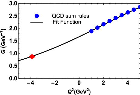
Figure 4: The sum rule predictions and fit function for the strong coupling $G(Q^{2})$. The point $Q^{2}=-m_{D_{s}}^{2}$ is shown by the red diamond.

Figure 5: The strong coupling $G=G(3~{}\mathrm{GeV}^{2})$ as a function of the Borel parameters $M_{1}^{2}$ and $M_{2}^{2}$ at $s_{0}=21.5~{}\mathrm{GeV}^{2}$ and $s_{0}^{\prime}=5.5~{}\mathrm{GeV}^{2}$.

Quantity	Value (in $\mathrm{MeV}$ units)
$m_{D_{s}}$	$1969.0\pm 1.4$
$m_{\eta_{c}}$	$2983.9\pm 0.4$
$m_{\eta^{\prime}}$	$957.78\pm 0.06$
$m_{\eta}$	$547.862\pm 0.017$
$f_{D_{s}}$	$249.9\pm 0.5$
$f_{\eta_{c}}$	$320\pm 40$

Table 1: Masses and decay constants of the mesons $D_{s}^{\pm}$, $\eta_{c}$, $\eta^{\prime}$, and $\eta$ which are employed in numerical calculations.

IV Processes $X\rightarrow\eta_{c}\eta^{\prime}$ and $X\rightarrow\eta_{c}\eta$

The processes $X\rightarrow\eta_{c}\eta^{\prime}$ and $X\rightarrow\eta_{c}\eta$, in general, can be studied by a manner described above. But, it is well known that due to $U(1)$ anomaly there is a mixing in the system of $\eta-\eta^{\prime}$ mesons Feldmann:1998vh . This phenomenon leads to some subtleties in the choice of the interpolating currents for these particles. The $\eta-\eta^{\prime}$ mixing can be described in the framework of different approaches: The physical particles $\eta$ and $\eta^{\prime}$ can be expressed using either the octet-singlet or quark-flavor bases of the flavor $SU_{f}(3)$ group. It turns out that mixing of the physical states, decay constants and higher twist distribution amplitudes in the $\eta-\eta^{\prime}$ system take simple forms in the quark-flavor basis $|\eta_{q}\rangle=(\overline{u}u+\overline{d}d)/\sqrt{2}$ and $|\eta_{s}\rangle=\overline{s}s$ Feldmann:1998vh ; Agaev:2014wna ; Agaev:2015faa . Therefore, for our purposes it is convenient to describe the mesons $\eta$ and $\eta^{\prime}$ in the quark-flavor basis.

Then, the physical mesons $\eta$ and $\eta^{\prime}$ are expressed using the basic states $|\eta_{q}\rangle$ and $|\eta_{s}\rangle$

$$\begin{pmatrix}\eta\\ \eta^{\prime}\end{pmatrix}=U(\varphi)\begin{pmatrix}|\eta_{q}\rangle\\ |\eta_{s}\rangle\end{pmatrix},$$ (35)

where

$$U(\varphi)=\begin{pmatrix}\cos\varphi&-\sin\varphi\\ \sin\varphi&\cos\varphi\end{pmatrix},$$ (36)

is the mixing matrix in $|\eta_{q}\rangle-|\eta_{s}\rangle$ basis with $\varphi$ being a mixing angle. This assumption on the state mixing implies that the same pattern applies to relevant currents, decay constants and wave functions as well.

In this context the interpolating currents for the mesons $\eta$ and $\eta^{\prime}$ are given by the expressions

$$J^{\eta}(x) = -\sin\varphi\overline{s}_{j}(x)i\gamma_{5}s_{j}(x),$$

$$J^{\eta^{\prime}}(x) = \cos\varphi\overline{s}_{j}(x)i\gamma_{5}s_{j}(x),$$ (37)

where $j$ is the color index. Let us emphasize that in Eq. (37), we write down only $\overline{s}s$ component of the currents, which contribute to the decays under analysis.

We begin our calculations from the decay $X\rightarrow\eta_{c}\eta^{\prime}$. In this case, one should explore the correlation function

$$\widetilde{\Pi}(p,p^{\prime}) = i^{2}\int d^{4}xd^{4}ye^{i(p^{\prime}y-px)}\langle 0|\mathcal{T}\{J^{\eta_{c}}(y)$$ (38)

$$\times J^{\eta^{\prime}}(0)J^{\dagger}(x)\}|0\rangle,$$

with $\ J^{\eta_{c}}(y)$ being the interpolating current of the meson $\eta_{c}$

$$\ J^{\eta_{c}}(x)=\overline{c}_{i}(x)i\gamma_{5}c_{i}(x).$$ (39)

The ground-state contribution to the correlation function $\widetilde{\Pi}(p,p^{\prime})$ in terms of the involved particles’ matrix elements has the form

$$\widetilde{\Pi}^{\mathrm{Phys}}(p,p^{\prime})=\frac{\langle 0|J^{\eta_{c}}|\eta_{c}(p^{\prime})\rangle\langle 0|J^{\eta^{\prime}}|\eta^{\prime}(q)\rangle}{(p^{2}-m^{2})(p^{\prime 2}-m_{\eta_{c}}^{2})}$$

$$\times\frac{\langle\eta^{\prime}(q)\eta_{c}(p^{\prime})|X(p)\rangle\langle X(p)|J^{\dagger}|0\rangle}{(q^{2}-m_{\eta^{\prime}}^{2})}+\cdots,$$

(40)

where the dots indicate effects of higher resonances and continuum states. The function $\widetilde{\Pi}^{\mathrm{Phys}}(p,p^{\prime})$ can be simplified by invoking the matrix elements of the mesons $\eta_{c}$ and $\eta^{\prime}$

$$\langle 0|J^{\eta_{c}}|\eta_{c}\rangle=\frac{m_{\eta_{c}}^{2}\ f_{\eta_{c}}}{2m_{c}},\$$

$$2m_{s}\langle\eta^{\prime}|\overline{s}i\gamma_{5}s|0\rangle=h_{\eta^{\prime}}^{s},$$ (41)

where $m_{\eta_{c}}$ and $\ f_{\eta_{c}}$ are the mass and decay constant of the $\eta_{c}$ meson. The twist-3 matrix element of the local operator $\overline{s}i\gamma_{5}s$ sandwiched between the meson $\eta^{\prime}$ and vacuum states is denoted by $h_{\eta^{\prime}}^{s}$ Agaev:2014wna .  The parameter $h_{\eta^{\prime}}^{s}$ complies with mixing effect, and we get

$$h_{\eta^{\prime}}^{s}=h_{s}\cos\varphi.$$ (42)

The parameter $h_{s}$ in Eq. (42) can be defined theoretically Agaev:2014wna , but for our analysis it is enough to use phenomenological values of $h_{s}$ and $\varphi$

$$h_{s} = (0.087\pm 0.006)~{}\mathrm{GeV}^{3},$$

$$\varphi = 39.3^{\circ}\pm 1.0^{\circ}.$$ (43)

The vertex $X\eta_{c}\eta^{\prime}$ is chosen in the following form

$$\langle\eta^{\prime}(q)\eta_{c}(p^{\prime})|X(p)\rangle=g_{1}(q^{2})p\cdot p^{\prime},$$ (44)

where $g_{1}$ is the strong coupling corresponding to the vertex $X\eta_{c}\eta^{\prime}$. Using these matrix elements, one can obtain a new expression for $\Pi^{\mathrm{Phys}}(p,p^{\prime})$

$$\widetilde{\Pi}^{\mathrm{Phys}}(p,p^{\prime})=g_{1}(q^{2})\frac{fmm_{\eta_{c}}^{2}\ f_{\eta_{c}}h_{s}\cos^{2}\varphi}{4m_{c}m_{s}{}(p^{2}-m^{2})}$$

$$\times\frac{1}{(p^{\prime 2}-m_{\eta_{c}}^{2})(q^{2}-m_{\eta^{\prime}}^{2})}\frac{m^{2}+m_{\eta_{c}}^{2}-q^{2}}{2}+\cdots.$$

The QCD side of the sum rule for $g_{1}(q^{2})$ is given by the formula

$$\widetilde{\Pi}^{\mathrm{OPE}}(p,p^{\prime})=-\cos\varphi\int d^{4}xd^{4}ye^{i(p^{\prime}y-px)}\epsilon\widetilde{\epsilon}$$

$$\times\mathrm{Tr}\left[\gamma_{5}S_{c}^{ib}(y-x)\gamma_{5}\widetilde{S}_{s}^{jc}(-x)\gamma_{5}\widetilde{S}_{s}^{nj}(x)\right.$$

$$\left.\times\gamma_{5}S_{c}^{mi}(x-y)\right],$$ (46)

The sum rule for the coupling $g_{1}(q^{2})$ is derived using Borel transformations of invariant amplitudes $\widetilde{\Pi}^{\mathrm{Phys}}(p^{2},p^{\prime 2},q^{2})$ and $\widetilde{\Pi}^{\mathrm{OPE}}(p^{2},p^{\prime 2},q^{2})$ and reads

$$g_{1}(q^{2}) = -\frac{8m_{c}m_{s}}{fmm_{\eta_{c}}^{2}\ f_{\eta_{c}}h_{s}\cos\varphi}\frac{q^{2}-m_{\eta_{c}}^{2}}{m^{2}+m_{\eta_{c}}^{2}-q^{2}}$$ (47)

$$\times e^{m^{2}/M_{1}^{2}}e^{m_{\eta_{c}}^{2}/M_{2}^{2}}\widetilde{\Pi}(\mathbf{M}^{2},\mathbf{s}_{0},q^{2}).$$

Here, $\widetilde{\Pi}(\mathbf{M}^{2},\mathbf{s}_{0},q^{2})$ is the Borel transformed and subtracted amplitude $\widetilde{\Pi}^{\mathrm{OPE}}(p^{2},p^{\prime 2},q^{2})$.

The coupling $g_{1}(q^{2})$ is calculated using the following Borel and continuum threshold parameters in the $\eta_{c}$ channel

$$M_{2}^{2}\in[3,4]~{}\mathrm{GeV}^{2},\ s_{0}^{\prime}\in[9.5,10.5]~{}\mathrm{GeV}^{2},$$ (48)

whereas as $M_{1}^{2}$ and $s_{0}$ for the $X$ channel, we employ Eq. (15). The strong coupling $g_{1}$ is defined at the mass shell of the $\eta^{\prime}$ meson. The fit function $\mathcal{G}_{1}(Q^{2})$ given by Eq. (30) has the parameters $\mathcal{G}_{1}^{0}=0.26~{}\mathrm{GeV}^{-1}$, $c_{1}^{1}=4.72$, and $c_{1}^{2}=-3.52$. Relevant computations yield

$$g_{1}\equiv\mathcal{G}_{1}(-m_{\eta^{\prime}}^{2})=(1.9\pm 0.3)\times 10^{-1}\ \mathrm{GeV}^{-1}.$$ (49)

The partial width of this decay can be found by means of the formula Eq. (32), in which one should make substitutions $G\rightarrow g_{1}$, $m_{D_{s}}^{2}\rightarrow m_{\eta_{c}}^{2}$ and $\lambda\left(m,m_{D_{s}},m_{D_{s}}\right)\rightarrow\widetilde{\lambda}\left(m,m_{\eta_{c}},m_{\eta^{\prime}}\right)$. Then, for the process $X\rightarrow\eta_{c}\eta^{\prime}$, we get

$$\Gamma\left[X\rightarrow\eta_{c}\eta^{\prime}\right]=(3.0\pm 0.7)~{}\mathrm{MeV}.$$ (50)

Analysis of the decay $X\rightarrow\eta_{c}\eta$ can be performed in a similar way. Omitting further details, let us write down predictions obtained for key quantities. Thus, the strong coupling $g_{2}$ at the vertex $X\eta_{c}\eta$ is determined by the equality

$$g_{2}\equiv|\mathcal{G}_{2}(-m_{\eta}^{2})|=(1.4\pm 0.2)\times 10^{-1}\ \mathrm{GeV}^{-1},$$ (51)

where parameters of the fit function are $\mathcal{G}_{2}^{0}=-0.15~{}\mathrm{GeV}^{-1}$, $c_{2}^{1}=5.76$, and $c_{2}^{2}=-4.44$. The partial width of the decay $X\rightarrow\eta_{c}\eta$ is

$$\Gamma\left[X\rightarrow\eta_{c}\eta\right]=(5.2\pm 1.1)~{}\mathrm{MeV}.$$ (52)

With this information at hands, it is not difficult to find the full width of the scalar tetraquark $X$

$$\Gamma_{\mathrm{X}}=(42.2\pm 12.0)~{}\mathrm{MeV}.$$ (53)

This estimate is in excellent agreement with the LHCb data.

V Concluding notes

In this article, we have calculated spectral parameters of the scalar tetraquark $X$ in the framework of the QCD two-point sum rule method. We evaluated also full width of $X$, by taking into account its decay modes $X\rightarrow D_{s}^{+}D_{s}^{-}$, $X\rightarrow\eta_{c}\eta^{\prime}$ and $X\rightarrow\eta_{c}\eta$. Our result for the mass $m=(3976\pm 85)~{}\mathrm{MeV}$ of the tetraquark $X$ overshoots the corresponding LHCb datum, but is compatible with $m_{\exp}$ provided one takes into account the corresponding theoretical and experimental errors. Our prediction for the full width $\Gamma_{\mathrm{X}}=(42.2\pm 12.0)~{}\mathrm{MeV}$ of $X$ is in excellent agreement with $\Gamma_{\mathrm{exp}}$ from Eq. (1).

In Ref. LHCb:2022vsv the LHCb Collaboration assumed that the resonance $X(3960)$ is composed of four $c\overline{c}s\overline{s}$ quarks. This assumption is relied on theoretical predictions of Ref. Chen:2017dpy , in which the authors used QCD sum rule method and different interpolating currents to find the mass spectra of the diquark-antidiquark states $qc\overline{q}\overline{c}$ and $sc\overline{s}\overline{c}$ with $J^{\mathrm{PC}}=0^{++}$ and $2^{++}$. Some of the currents used there indeed led to estimations which are comparable with $m_{\mathrm{exp}}$ if one includes into consideration the ambiguities of the analysis.

In the context of the sum rule approach, $X(3960)$ was modeled as a $D_{s}^{+}D_{s}^{-}$ molecule state Xin:2022bzt , as well. In accordance with this paper, the mass of such hadronic molecule is equal to $(3980\pm 100)~{}\mathrm{MeV}$ being in agreement with the LHCb data. It is worth noting that in Refs. Chen:2017dpy ; Xin:2022bzt the authors did not investigate quantitatively widths of the diquark-antidiquark or molecule states considered there, which is crucial to draw a conclusion about the inner organization of $X(3960)$.

The results for $m$ and $\Gamma_{\mathrm{X}}$ obtained in the present article allow us to consider $X(3960)$ as a candidate to a scalar diquark-antidiquark exotic meson. At the same time, a molecule model for $X(3960)$ should be studied in a more detailed form: There is a necessity to evaluate full width of a molecule state. Only after such comprehensive analysis it is possible to make a choice between the competing models.

*

Appendix A The propagators $S_{q(Q)}(x)$ and the invariant amplitude $\Pi(M^{2},s_{0})$

In the current article, for the light quark propagator $S_{q}^{ab}(x)$, we employ the following expression

$$S_{q}^{ab}(x)=i\delta_{ab}\frac{\not{x}}{2\pi^{2}x^{4}}-\delta_{ab}\frac{m_{q}}{4\pi^{2}x^{2}}-\delta_{ab}\frac{\langle\overline{q}q\rangle}{12}+i\delta_{ab}\frac{\not{x}m_{q}\langle\overline{q}q\rangle}{48}-\delta_{ab}\frac{x^{2}}{192}\langle\overline{q}g_{s}\sigma Gq\rangle$$

$$+i\delta_{ab}\frac{x^{2}\not{x}m_{q}}{1152}\langle\overline{q}g_{s}\sigma Gq\rangle-i\frac{g_{s}G_{ab}^{\alpha\beta}}{32\pi^{2}x^{2}}\left[\not{x}{\sigma_{\alpha\beta}+\sigma_{\alpha\beta}}\not{x}\right]-i\delta_{ab}\frac{x^{2}\not{x}g_{s}^{2}\langle\overline{q}q\rangle^{2}}{7776}$$

$$-\delta_{ab}\frac{x^{4}\langle\overline{q}q\rangle\langle g_{s}^{2}G^{2}\rangle}{27648}+\cdots.$$ (A.54)

For the heavy quark $Q=c$, we use the propagator $S_{Q}^{ab}(x)$

$$S_{Q}^{ab}(x)=i\int\frac{d^{4}k}{(2\pi)^{4}}e^{-ikx}\Bigg{\{}\frac{\delta_{ab}\left({\not{k}}+m_{Q}\right)}{k^{2}-m_{Q}^{2}}-\frac{g_{s}G_{ab}^{\alpha\beta}}{4}\frac{\sigma_{\alpha\beta}\left({\not{k}}+m_{Q}\right)+\left({\not{k}}+m_{Q}\right)\sigma_{\alpha\beta}}{(k^{2}-m_{Q}^{2})^{2}}$$

$$+\frac{g_{s}^{2}G^{2}}{12}\delta_{ab}m_{Q}\frac{k^{2}+m_{Q}{\not{k}}}{(k^{2}-m_{Q}^{2})^{4}}+\frac{g_{s}^{3}G^{3}}{48}\delta_{ab}\frac{\left({\not{k}}+m_{Q}\right)}{(k^{2}-m_{Q}^{2})^{6}}\left[{\not{k}}\left(k^{2}-3m_{Q}^{2}\right)+2m_{Q}\left(2k^{2}-m_{Q}^{2}\right)\right]\left({\not{k}}+m_{Q}\right)+\cdots\Bigg{\}}.$$

Here, we have used the short-hand notations

$$G_{ab}^{\alpha\beta}\equiv G_{A}^{\alpha\beta}\lambda_{ab}^{A}/2,\ \ G^{2}=G_{\alpha\beta}^{A}G_{A}^{\alpha\beta},\ G^{3}=f^{ABC}G_{\alpha\beta}^{A}G^{B\beta\delta}G_{\delta}^{C\alpha},$$ (A.56)

where $G_{A}^{\alpha\beta}$ is the gluon field strength tensor, $\lambda^{A}$ and $f^{ABC}$ are the Gell-Mann matrices and structure constants of the color group $SU_{c}(3)$, respectively. The indices $A,B,C$ run in the range $1,2,\ldots 8$.

The invariant amplitude $\Pi(M^{2},s_{0})$ obtained after the Borel transformation and subtraction procedures is given by Eq. (9)

$$\Pi(M^{2},s_{0})=\int_{4\mathcal{M}^{2}}^{s_{0}}ds\rho^{\mathrm{OPE}}(s)e^{-s/M^{2}}+\Pi(M^{2}),$$

where the spectral density $\rho^{\mathrm{OPE}}(s)$ and the function $\Pi(M^{2})$ are determined by the expressions

$$\rho^{\mathrm{OPE}}(s)=\rho^{\mathrm{pert.}}(s)+\sum_{N=3}^{8}\rho^{\mathrm{DimN}}(s),\ \ \Pi(M^{2})=\sum_{N=6}^{10}\Pi^{\mathrm{DimN}}(M^{2}),$$ (A.57)

respectively. The components of $\rho^{\mathrm{OPE}}(s)$ and $\Pi(M^{2})$ are given by the formulas

$$\rho^{\mathrm{DimN}}(s)=\int_{0}^{1}d\alpha\int_{0}^{1-a}d\beta\rho^{\mathrm{DimN}}(s,\alpha,\beta),\ \ \rho^{\mathrm{DimN}}(s)=\int_{0}^{1}d\alpha\rho^{\mathrm{DimN}}(s,\alpha),$$ (A.58)

and

$$\Pi^{\mathrm{DimN}}(M^{2})=\int_{0}^{1}d\alpha\int_{0}^{1-a}d\beta\Pi^{\mathrm{DimN}}(M^{2},\alpha,\beta),\ \ \Pi^{\mathrm{DimN}}(M^{2})=\int_{0}^{1}d\alpha\Pi^{\mathrm{DimN}}(M^{2},\alpha).$$ (A.59)

In Eqs. (A.58) and (A.59) variables $\alpha$ and $\beta$ are Feynman parameters.

The perturbative and nonperturbative components of the spectral density $\rho^{\mathrm{pert.}}(s,\alpha,\beta)$ and $\rho^{\mathrm{Dim3(4,5,6,7,8)}}(s,\alpha,\beta)$  have the forms:

$$\rho^{\mathrm{pert.}}(s,\alpha,\beta)=\frac{\Theta(L)L^{2}}{512\pi^{6}(\beta-1)^{4}N_{1}^{4}N_{2}}\left\{2(\beta-1)^{2}N_{3}\left[-\alpha\beta N_{3}+3m_{c}m_{s}(\alpha+\beta)N_{1}^{2}\right]\right.$$

$$\left.+4(\beta-1)N_{1}^{2}L\left[-\alpha\beta N_{3}+m_{c}m_{s}(\alpha+\beta)N_{1}^{2}\right]-\alpha\beta N_{1}^{4}L^{2}\right\},$$ (A.60)

$$\rho^{\mathrm{Dim3}}(s,\alpha,\beta)=-\frac{\langle\overline{s}s\rangle\Theta(L)}{16\pi^{4}(\beta-1)^{2}N_{1}^{6}}\left\{m_{s}(\beta-1)^{2}\alpha\beta N_{2}N_{3}^{2}+(\beta-1)N_{1}^{2}\left[6m_{s}\alpha\beta N_{2}N_{3}+2m_{c}^{2}m_{s}N_{1}^{3}\right.\right.$$

$$\left.-m_{c}s\alpha\beta L(\beta^{4}+\alpha^{2}(\alpha-1)^{2}+\beta^{3}(3\alpha-2)+\alpha\beta(2-5\alpha+3\alpha^{2})+\beta^{2}(1-5\alpha+4\alpha^{2}))\right]$$

$$\left.-N_{1}^{4}\left[-3m_{s}\alpha\beta N_{2}+m_{c}L^{2}(\beta^{3}+2\beta\alpha(\alpha-1)+\alpha^{2}(\alpha-1)+\beta^{2}(2\alpha-1)\right]\right\},$$ (A.61)

$$\rho^{\mathrm{Dim4}}(s,\alpha,\beta)=\frac{\langle\alpha_{s}G^{2}/\pi\rangle\Theta(L)}{4608\pi^{4}(\beta-1)^{2}N_{1}^{5}N_{2}^{2}}\left\{\alpha\beta(\beta-1)^{2}\left[-6m_{c}m_{s}(\beta^{3}+\beta^{2}(\alpha-1)+\beta^{2}\alpha+\alpha^{2}(\alpha-1))\right.\right.$$

$$\times(3N_{2}N_{3}+2m_{c}^{2}N_{1})+N_{2}N_{3}(\alpha+\beta)(54N_{2}N_{3}+m_{c}^{2}(\beta^{4}-\beta^{3}+\beta^{2}\alpha^{2}+\alpha^{3}(\alpha-1))/N_{1}$$

$$+sm_{c}N_{2}^{2}\left(11m_{c}\alpha\beta(\alpha^{3}+\beta^{3})+6m_{s}\left(2\beta^{5}-73\beta^{3}\alpha(\alpha-1)+2\alpha^{4}(\alpha-1)-\beta^{4}(2+37\alpha)+\beta^{2}\alpha\right.\right.$$

$$\left.\left.\left.\times(-36+108\alpha-73\alpha^{2})+\beta\alpha^{2}(-36+73\alpha-37\alpha^{2})\right)\right)\right]+12N_{1}^{2}(\beta-1)L\left[27N_{2}^{2}N_{3}\alpha\beta(\alpha+\beta)/N_{1}\right.$$

$$+m_{c}^{2}\alpha\beta(\alpha^{3}+\beta^{3})N_{2}+m_{c}m_{s}\left(2\beta^{6}+2\alpha^{4}(\alpha-1)^{2}-\beta^{5}(4+35\alpha)+\beta^{3}\alpha(-109+254\alpha-146\alpha^{2})\right.$$

$$\left.\left.+\beta^{4}(2+108\alpha-110\alpha^{2})+\beta\alpha^{2}(36-109\alpha+108\alpha^{2}-35\alpha^{3})-2\beta^{2}\alpha(-18+90\alpha-127\alpha^{2}+55\alpha^{3})\right)\right]$$

$$\left.+162L^{2}\alpha\beta N_{1}^{3}N_{2}(\beta^{2}+\alpha(\alpha-1)+\beta(2\alpha-1))\right\},$$ (A.62)

$$\rho^{\mathrm{Dim5}}(s,\alpha,\beta)=\frac{\langle\overline{s}g_{s}\sigma Gs\rangle\alpha\beta N_{2}\Theta(L)}{64\pi^{4}(\beta-1)N_{1}^{6}}\left\{(\beta-1)\left[13m_{s}\alpha\beta N_{2}N_{3}+4m_{c}^{2}m_{s}N_{1}^{3}-6m_{c}s\alpha\beta\left(\beta^{4}\right.\right.\right.$$

$$\left.\left.+\alpha^{2}(\alpha-1)^{2}+\beta^{3}(3\alpha-2)+\beta\alpha(2-5\alpha+3\alpha^{2})+\beta^{2}(1-5\alpha+4\alpha^{2})\right)\right]-2N_{1}^{2}L\left[-8m_{s}\alpha\beta N_{2}\right.$$

$$\left.\left.+3m_{c}(\beta^{3}+2\beta\alpha(\alpha-1)+\alpha^{2}(\alpha-1)+\beta^{2}(2\alpha-1))\right]\right\},$$ (A.63)

$$\rho^{\mathrm{Dim6}}(s,\alpha,\beta)=\frac{\Theta(L)}{829440\pi^{6}(\beta-1)^{2}N_{1}^{5}N_{2}^{2}}\left\{3840g_{s}^{2}\langle\overline{s}s\rangle^{2}\pi^{2}(\beta-1)\alpha\beta N_{2}^{4}[s(\beta-1)\alpha\beta N_{2}+N_{1}^{2}L]\right.$$

$$-27\langle g_{s}^{3}G^{3}\rangle m_{c}^{2}\beta^{5}(\beta-1)^{2}\left[2(\beta-1)\beta\alpha N_{2}-2\alpha\left(-5\beta^{3}+\beta^{2}(10-3\alpha)+2\alpha(\alpha-1)^{2}\right.\right.$$

$$\left.\left.\left.+\beta(-5+\alpha+4\alpha^{2})\right)\right]\right\},$$ (A.64)

$$\rho_{1}^{\mathrm{Dim7}}(s,\alpha,\beta)=\frac{\langle\alpha_{s}G^{2}/\pi\rangle\langle\overline{s}s\rangle\Theta(L)}{1152\pi^{2}(\beta-1)N_{1}^{4}}\left\{90m_{s}\left(\beta-1\right)\alpha\beta(\alpha+\beta)N_{2}^{2}+18m_{s}(\beta-1)\alpha\beta N_{2}\right.$$

$$\times\left[\beta^{2}+\alpha(\alpha-1)+\beta(2\alpha-1)\right]+8m_{c}\left[2\beta^{6}+2\alpha^{4}(\alpha-1)^{2}-\beta^{5}(4+19\alpha)+\beta^{4}(2+56\alpha-37\alpha^{2})\right.$$

$$\left.\left.+\beta^{3}\alpha(-55+91\alpha-37\alpha^{2})+\beta^{2}\alpha(18-72\alpha+74\alpha^{2}-17\alpha^{3})+\beta\alpha^{2}(18-37\alpha+15\alpha^{2}+4\alpha^{3})\right]\right\},$$ (A.65)

$$\rho^{\mathrm{Dim8}}(s,\alpha,\beta)=-\frac{\langle\alpha_{s}G^{2}/\pi\rangle^{2}\alpha^{2}\beta^{2}N_{2}\Theta(L)}{512\pi^{2}N_{1}^{4}}.$$ (A.66)

The function $\rho_{2}^{\mathrm{Dim7}}(s,\alpha)$ is determined by the expression

$$\rho_{2}^{\mathrm{Dim7}}(s,\alpha)=-\frac{\langle\alpha_{s}G^{2}/\pi\rangle\langle\overline{s}s\rangle m_{c}}{288\pi^{2}}\Theta(\widetilde{L}).$$ (A.67)

Components of $\Pi(M^{2})$ are

$$\Pi^{\mathrm{Dim6}}(M^{2},\alpha,\beta)=\frac{\langle g_{s}^{3}G^{3}\rangle m_{c}^{3}\beta^{4}(\beta-1)}{92160M^{4}\pi^{6}N_{1}^{6}N_{2}}\exp\left[-\frac{m_{c}^{2}(\alpha+\beta)N_{1}}{M^{2}\alpha\beta N_{2}}\right]\left\{-\left[2m_{c}^{5}\alpha\beta(\beta-1)^{2}(\alpha+\beta)^{2}\right.\right.$$

$$\left.+3m_{c}M^{4}\alpha\beta N_{1}^{2}\right]\left[3\beta^{3}+\beta\alpha(\alpha-2)-\alpha^{2}(\alpha-1)+\beta^{2}(2\alpha-3)\right]+6m_{s}M^{4}N_{1}^{3}\left[8\beta^{3}+\beta\alpha(\alpha-3)\right.$$

$$\left.+\alpha^{2}(\alpha-1)+\beta^{2}(3\alpha-8)\right]+6m_{c}^{2}m_{s}M^{2}(\beta-1)N_{1}^{2}\left[8\beta^{4}+2\beta\alpha^{2}(\alpha-2)+\alpha^{3}(\alpha-1)\right.$$

$$\left.+\beta^{2}\alpha(4\alpha-11)+\beta^{3}(11\alpha-8)\right]+6m_{c}^{4}m_{s}(\beta-1)^{2}\left[2\beta^{7}-\alpha^{5}(\alpha-1)^{2}+\beta^{6}(5\alpha-4)\right.$$

$$+\beta^{3}\alpha^{2}(2+11\alpha-14\alpha^{2})+\beta^{4}\alpha(5-4\alpha-7\alpha^{2})+\beta\alpha^{4}(-4+9\alpha-5\alpha^{2})+2\beta^{5}(1-5\alpha+\alpha^{2})$$

$$\left.-4\beta^{2}\alpha^{3}(1-4\alpha+3\alpha^{2})\right]+3m_{c}^{3}M^{2}\alpha\beta(\beta-1)\left[3\beta^{6}-\beta\alpha^{4}(\alpha-1)-\alpha^{4}(\alpha-1)^{2}+\beta^{5}(8\alpha-6)\right.$$

$$\left.\left.+2\beta^{2}\alpha^{2}(3-4\alpha+\alpha^{2})+\beta^{3}\alpha(8-17\alpha+8\alpha^{2})+\beta^{4}(3-16\alpha+11\alpha^{2})\right]\right\},$$ (A.68)

$$\Pi^{\mathrm{Dim7}}(M^{2},\alpha,\beta)=\frac{\langle\alpha_{s}G^{2}/\pi\rangle\langle\overline{s}s\rangle m_{c}^{2}}{576\pi^{2}M^{4}N_{1}^{7}}\exp\left[-\frac{m_{c}^{2}(\alpha+\beta)N_{1}}{M^{2}\alpha\beta N_{2}}\right]\left\{-2m_{c}M^{2}\alpha\beta(\beta-1)\left[m_{c}^{2}(\alpha+\beta)(\beta-1)\right.\right.$$

$$\left.+M^{2}N_{1}\right]\left[2\beta^{6}+2\alpha^{4}(\alpha-1)^{2}+\beta^{5}(5\alpha-4)+\beta\alpha^{3}(4-9\alpha+5\alpha^{2})+\alpha^{2}\beta^{2}(4-13\alpha+9\alpha^{2})\right.$$

$$\left.+\beta^{4}(2-9\alpha+9\alpha^{2})+\beta^{3}\alpha(4-13\alpha+10\alpha^{2})\right]+m_{s}\left[2m_{c}^{4}(\beta-1)^{3}\alpha\beta(\alpha+\beta)^{3}(\beta^{3}-\beta^{2}+\beta\alpha+\alpha^{2}(\alpha-1))\right.$$

$$+m_{c}^{2}M^{2}(\beta-1)^{2}\alpha\beta(\alpha+\beta)^{2}\left(7\beta^{5}+3\beta^{4}(5\alpha-6)+\alpha^{2}(\alpha-1)^{2}(7\alpha-4)+\beta^{3}(15-35\alpha+23\alpha^{2})\right.$$

$$\left.+\alpha\beta(-8+28\alpha-35\alpha^{2}+15\alpha^{3})+\beta^{2}(-4+28\alpha-47\alpha^{2}+23\alpha^{3})\right)-M^{4}N_{1}^{2}\left(8\beta^{7}+8\alpha^{4}(\alpha-1)^{3}+3\beta^{6}(3\alpha-8)\right.$$

$$+\beta^{5}(24-30\alpha+17\alpha^{2})+3\beta\alpha^{3}(-4+15\alpha-19\alpha^{2}+8\alpha^{3})+3\beta^{3}\alpha(-4+12\alpha-20\alpha^{2}+11\alpha^{3})$$

$$\left.\left.\left.+\beta^{4}(-8+33\alpha-45\alpha^{2}+24\alpha^{3})+\beta^{2}\alpha^{2}(-8+48\alpha-70\alpha^{2}+33\alpha^{3})\right)\right]\right\},$$ (A.69)

$$\Pi^{\mathrm{Dim8}}(M^{2},\alpha,\beta)=-\frac{\langle\alpha_{s}G^{2}/\pi\rangle^{2}\alpha\beta(\beta-1)}{82944\pi^{2}M^{6}N_{1}^{8}N_{2}}\exp\left[-\frac{m_{c}^{2}(\alpha+\beta)N_{1}}{M^{2}\alpha\beta N_{2}}\right]\left\{2m_{c}^{7}(\beta-1)^{3}\alpha^{3}\beta^{3}(\alpha+\beta)^{2}\right.$$

$$-6m_{c}^{6}m_{s}(\beta-1)^{3}\alpha^{2}\beta^{2}(\alpha+\beta)^{3}N_{2}+81m_{c}M^{6}\alpha\beta N_{1}^{3}\left[\beta^{3}+\beta^{2}(\alpha-1)+\beta\alpha^{2}+\alpha^{2}(\alpha-1)\right]+216m_{s}M^{6}N_{1}^{3}$$

$$\times\left[\beta^{5}+\beta^{4}(\alpha-2)-\beta^{3}(\alpha-1)+\beta\alpha^{3}(\alpha-1)+\alpha^{3}(\alpha-1)^{2}\right]+81m_{c}^{3}M^{4}(\beta-1)\alpha\beta N_{1}^{2}\left[\beta^{4}+\alpha^{3}(\alpha-1)\right.$$

$$\left.+\beta^{3}(2\alpha-1)+\beta^{2}\alpha(2\alpha-1)+\beta\alpha^{2}(2\alpha-1)\right]+216m_{c}^{2}m_{s}M^{4}(\beta-1)N_{1}^{2}\left[\beta^{6}+2\beta^{5}(\alpha-1)-\beta^{3}\alpha(\alpha-1)\right.$$

$$\left.+\beta^{2}\alpha^{3}(\alpha-1)+\alpha^{4}(\alpha-1)^{2}+\beta^{4}(1-3\alpha+\alpha^{2})+\beta\alpha^{3}(1-3\alpha+2\alpha^{2})\right]+54m_{c}^{5}M^{2}(\beta-1)^{2}\alpha\beta(\alpha+\beta)^{2}$$

$$\times\left[\beta^{5}+2\beta^{4}(\alpha-1)+\alpha^{3}(\alpha-1)+\beta\alpha^{2}(1-3\alpha+2\alpha^{2})+\beta^{2}\alpha(1-4\alpha+3\alpha^{2})+\beta^{3}(1-3\alpha+3\alpha^{2}\right]$$

$$-12m_{c}^{4}m_{s}M^{2}(\beta-1)^{2}\alpha\beta\left[9\beta^{7}+9\alpha^{4}(\alpha-1)^{3}+4\beta\alpha^{3}(\alpha-1)(13\alpha-9)+\beta^{6}(52\alpha-27)+\beta^{5}\left(27-140\alpha\right.\right.$$

$$\left.+138\alpha^{2}\right)+3\beta^{2}\alpha^{2}(-18+79\alpha-107\alpha^{2}+46\alpha^{3})+\beta^{3}\alpha(-36+237\alpha-416\alpha^{2}+215\alpha^{3})$$

$$\left.\left.+\beta^{4}(-9+124\alpha-321\alpha^{2}+215\alpha^{3})\right]\right\}.$$ (A.70)

The terms $\mathrm{Dim9}$ and $\mathrm{Dim10}$ are exclusively of the type (A.59) and have two components $\Pi_{1}^{\mathrm{DimN}}(M^{2},\alpha,\beta)$ and $\Pi_{2}^{\mathrm{DimN}}(M^{2},\alpha)$ presented below:

$$\Pi_{1}^{\mathrm{Dim9}}(M^{2},\alpha,\beta)=\frac{m_{c}(\beta-1)}{17280\pi^{4}M^{8}N_{1}^{10}}\exp\left[-\frac{m_{c}^{2}(\alpha+\beta)N_{1}}{M^{2}\alpha\beta N_{2}}\right]\left\{5\langle\alpha_{s}G^{2}/\pi\rangle\langle\overline{s}g_{s}\sigma Gs\rangle M^{2}\pi^{2}N_{1}^{2}N_{2}\right.$$

$$\times\left[2m_{c}^{5}m_{s}(\beta-1)^{3}\alpha\beta(\alpha+\beta)^{3}\left(\beta^{3}-\beta^{2}+\beta\alpha+\alpha^{2}(\alpha-1)\right)+6M^{6}N_{1}^{3}\left(\beta^{5}-\beta^{4}+\alpha^{4}(\alpha-1)\right)\right.$$

$$+6m_{c}^{2}M^{4}(\beta-1)N_{1}^{2}\left(\beta^{6}+\beta^{5}(\alpha-1)-\beta^{4}\alpha+\beta\alpha^{4}(\alpha-1)+\alpha^{5}(\alpha-1)\right)-3m_{c}^{4}M^{2}(\beta-1)^{2}\alpha\beta$$

$$\times\left(2\beta^{7}+2\alpha^{5}(\alpha-1)^{2}+\beta^{6}(7\alpha-4)+\beta\alpha^{4}(6-13\alpha+7\alpha^{2})+2\beta^{2}\alpha^{3}(4-11\alpha+7\alpha^{2})\right.$$

$$\left.\left.+\beta^{5}(2-13\alpha+14\alpha^{2})+\beta^{3}\alpha^{2}(8-26\alpha+19\alpha^{2})+\beta^{4}\alpha(6-22\alpha+19\alpha^{2})\right)\right]$$

$$+3\langle g_{s}^{3}G^{3}\rangle\langle\overline{s}s\rangle m_{c}^{3}(\beta-1)^{2}\left[m_{c}M^{4}N_{1}^{4}\left(6\beta^{6}+8\beta^{5}\alpha+3\beta^{4}\alpha^{2}+3\beta^{2}\alpha^{4}+8\beta\alpha^{5}+6\alpha^{6}\right)\right.$$

$$-8m_{s}M^{4}N_{1}^{4}\left(2\beta^{6}+3\beta^{4}\alpha(\alpha-1)+3\beta^{2}\alpha^{4}+3\beta\alpha^{4}(\alpha-1)+2\alpha^{5}(\alpha-1)+\beta^{5}(3\alpha-2)\right)$$

$$-m_{c}^{4}m_{s}(\beta-1)^{2}\alpha\beta(\alpha+\beta)^{3}\left(3\beta^{7}+2\beta^{6}(\alpha-3)-\beta^{3}\alpha^{3}(\alpha-3)+\beta^{2}\alpha^{4}(\alpha-1)+3\alpha^{5}(\alpha-1)^{2}\right.$$

$$\left.+\beta^{5}(3-\alpha+\alpha^{2})-\beta^{4}\alpha(1+\alpha+\alpha^{2})+\beta\alpha^{4}(-1-\alpha+2\alpha^{2})\right)-m_{c}^{2}m_{s}M^{2}(\beta-1)N_{1}^{2}$$

$$\times\left(4\beta^{9}-3\beta\alpha^{7}(\alpha-1)+4\alpha^{7}(\alpha-1)^{2}-\beta^{8}(8+3\alpha)-3\beta^{6}\alpha^{2}(7\alpha-8)+\beta^{5}\alpha^{2}(-12+29\alpha-25\alpha^{2})\right.$$

$$\left.+\beta^{4}\alpha^{3}(-8+32\alpha-25\alpha^{2})+\beta^{3}\alpha^{4}(-8+29\alpha-21\alpha^{2})+\beta^{7}(4+3\alpha-15\alpha^{2})-3\beta^{2}\alpha^{5}(4-8\alpha+5\alpha^{2})\right)$$

$$+m_{c}^{3}M^{2}(\beta-1)N_{1}^{2}\left(2\beta^{9}+\beta^{5}\alpha^{3}(3-5\alpha)+\beta^{4}\alpha^{4}(2-5\alpha)+\beta^{3}\alpha^{5}(3-7\alpha)+3\beta\alpha^{7}(\alpha-1)\right.$$

$$\left.\left.\left.+2\alpha^{8}(\alpha-1)-3\beta^{7}\alpha(1+\alpha)+\beta^{8}(3\alpha-2)+\beta^{6}\alpha^{2}(1-7\alpha)+\beta^{2}\alpha^{6}(1-3\alpha)\right)\right]\right\},$$ (A.71)

$$\Pi_{2}^{\mathrm{Dim9}}(M^{2},\alpha)=\frac{\langle\alpha_{s}G^{2}/\pi\rangle\langle\overline{s}g_{s}\sigma Gs\rangle m_{c}}{1152M^{4}\pi^{2}\alpha^{4}(\alpha-1)^{2}}\exp\left[-\frac{m_{c}^{2}}{M^{2}\alpha(1-\alpha)}\right]\left[2m_{c}^{3}m_{s}(\alpha-1)\right.$$

$$\left.-9m_{c}^{2}M^{2}\alpha^{2}(\alpha-1)+9M^{4}\alpha^{3}(\alpha-1)^{2}+4m_{c}m_{s}M^{2}\alpha(1-\alpha-2\alpha^{2}+3\alpha^{3})\right],$$ (A.72)

$$\Pi_{1}^{\mathrm{Dim10}}(M^{2},\alpha,\beta)=-\frac{m_{c}^{3}\alpha\beta(\beta-1)^{3}}{3645\cdot 10^{11}M^{10}\pi^{4}N_{1}^{11}N_{2}}\exp\left[-\frac{m_{c}^{2}(\alpha+\beta)N_{1}}{M^{2}\alpha\beta N_{2}}\right]\left\{320g_{s}^{2}\langle\overline{s}s\rangle^{2}\pi^{2}m_{c}^{3}M^{4}\right.$$

$$\times(\beta-1)(\beta^{2}-\beta\alpha+\alpha^{2})\left[\beta^{4}+\alpha^{2}(\alpha-1)^{2}+\beta^{3}(3\alpha-2)+\beta\alpha(2-5\alpha+3\alpha^{2})+\beta^{2}(1-5\alpha+4\alpha^{2})\right]^{3}$$

$$+9\langle g_{s}^{3}G^{3}\rangle\alpha^{2}\beta^{2}\left[12m_{c}^{3}M^{4}\alpha^{2}\beta^{2}(\beta-1)N_{1}^{3}+18m_{s}M^{6}(\alpha+\beta)N_{1}^{5}-m_{c}^{7}\alpha\beta(\beta-1)^{3}(\alpha+\beta)^{2}\right.$$

$$\times\left(3\beta^{4}+\beta^{3}(\alpha-3)+\beta\alpha^{2}(\alpha-1)+3\alpha^{3}(\alpha-1)+\beta^{2}\alpha(2\alpha-1)\right)-6m_{c}^{2}m_{s}M^{4}(\beta-1)N_{1}^{3}\left(5\beta^{4}\right.$$

$$\left.+22\beta\alpha^{2}(\alpha-1)+5\alpha^{3}(\alpha-1)+2\beta^{2}\alpha(19\alpha-11)+\beta^{3}(22\alpha-5)\right)+3m_{c}^{6}m_{s}(\beta-1)^{3}(\alpha+\beta)^{2}\left(5\beta^{6}\right.$$

$$+3\beta\alpha^{4}(\alpha-1)+5\alpha^{4}(\alpha-1)^{2}+\beta^{5}(3\alpha-10)-2\beta^{3}\alpha^{2}(7\alpha-8)+\beta^{4}(5-3\alpha-6\alpha^{2})-2\alpha^{2}\beta^{2}$$

$$\left.\times(5-8\alpha+3\alpha^{2})\right)+3m_{c}^{5}M^{2}\alpha\beta(\beta-1)^{2}\left(3\beta^{7}+\beta^{4}\alpha(5-4\alpha)+4\beta^{2}\alpha^{4}(\alpha-1)+5\beta\alpha^{4}(\alpha-1)^{2}\right.$$

$$\left.+3\alpha^{5}(\alpha-1)^{2}+\beta^{6}(5\alpha-6)+\beta^{5}(3-10\alpha+4\alpha^{2})\right)-3m_{c}^{4}m_{s}M^{2}(\beta-1)^{2}\left(13\beta^{9}+13\alpha^{6}(\alpha-1)^{3}\right.$$

$$+\beta^{8}(20\alpha-39)+\beta\alpha^{5}(\alpha-1)^{2}(20\alpha-11)-\beta^{2}\alpha^{4}(\alpha-1)^{2}(45\alpha-73)+\beta^{7}(39-51\alpha-45\alpha^{2})$$

$$+\beta^{4}\alpha^{2}(73-510\alpha+808\alpha^{2}-371\alpha^{3})+\beta^{6}(-13+42\alpha+163\alpha^{2}-211\alpha^{3})$$

$$\left.\left.\left.+\beta^{3}\alpha^{3}(142-510\alpha+579\alpha^{2}-211\alpha^{3})-\beta^{5}\alpha(11+191\alpha-579\alpha^{2}+371\alpha^{3})\right)\right]\right\},$$ (A.73)

and

$$\Pi_{2}^{\mathrm{Dim10}}(M^{2},\alpha)=\frac{\langle\alpha_{s}G^{2}/\pi\rangle g_{s}^{2}\langle\overline{s}s\rangle^{2}m_{c}^{3}m_{s}}{23328M^{4}\pi^{2}(\alpha-1)^{3}}\exp\left[-\frac{m_{c}^{2}}{M^{2}\alpha(1-\alpha)}\right].$$ (A.74)

In expressions above, $\Theta(x)$ is Unit Step function. We have also used the following short-hand notations

$$N_{1} = \beta^{2}+(\alpha+\beta)(\alpha-1),\ \ \ \ \ N_{2}=\alpha+\beta-1,\ \ N_{3}=s\alpha\beta N_{2},\$$

$$\ \ \ L \equiv L(s,\alpha,\beta)=\frac{(\beta-1)\left[N_{3}-m_{c}^{2}(\alpha+\beta)N_{1}\right]}{N_{1}^{2}},\ \widetilde{L}\equiv\widetilde{L}(s,\alpha)=s\alpha(1-\alpha)-m_{c}^{2}.$$ (A.75)

References

(1) The LHCb Collaboration,
arXiv:2210.15153 [hep-ex].
(2) R. Aaij et al. [LHCb Collaboration],
Phys. Rev. Lett. 118, 022003 (2017);
R. Aaij et al. [LHCb Collaboration],
Phys. Rev. D 95, 012002 (2017).
(3) T. Aaltonen et al. [CDF Collaboration],
Phys. Rev. Lett. 102, 242002 (2009).
(4) S. Chatrchyan et al. [CMS
Collaboration],
Phys. Lett. B 734, 261 (2014).
(5) V. M. Abazov et al. [D0 Collaboration],
Phys. Rev. D 89, 012004 (2014).
(6) R. Aaij et al. [LHCb Collaboration],
Phys. Rev. Lett. 127, 082001 (2021).
(7) J. Nieves, and M. P. Valderrama,
Phys. Rev. D 86, 056004 (2012).
(8) Z. G. Wang, Eur. Phys. J. C 74, 2874 (2014).
(9) R. F. Lebed, and A. D. Polosa, Phys. Rev. D
93, 094024 (2016).
(10) W. Chen, H. X. Chen, X. Liu, T. G. Steele, and
S. L. Zhu, Phys. Rev. D 96, 114017 (2017).
(11) L. Meng, B. Wang, and S. L. Zhu,
Sci. Bull. 66, 1288 (2021).
(12) S. S. Agaev, K. Azizi and H. Sundu,
Phys. Rev. D 95, 114003 (2017).
(13) H. Sundu, S. S. Agaev and K. Azizi,
Phys. Rev. D 98, 054021 (2018).
(14) S. S. Agaev, K. Azizi and H. Sundu,
Phys. Rev. D 106, 014025 (2022).
(15) C. Chen, and E. S. Norella,
https://indico.cern.ch/event/1176505/
(16) M. Bayar, A. Feijoo, and E. Oset,
arXiv:2207.08490 [hep-ph].
(17) T. Ji, X. K. Dong, M. Albaladejo, M. L. Du, F. K. Guo,
and J.Nieves, arXiv:2207.08563 [hep-ph].
(18) Q. Xin, Z. G. Wang, and X. S. Yang,
AAPPS Bull. 32, 37 (2022).
(19) J. M. Xie, M. Z. Liu, and L. S. Geng,
Phys. Rev. D 107, 016003 (2023).
(20) R. Chen, and Q.Huang,
arXiv:2209.05180 [hep-ph].
(21) D. Guo, J. Z. Wang, D. Y. Chen, and X. Liu,
Phys. Rev. D 106, 094037 (2022).
(22) D. Guo, J. Li, J. Zhao, and L. He,
(23) M. A. Shifman, A. I. Vainshtein and V. I. Zakharov,
Nucl. Phys. B 147, 385 (1979).
(24) M. A. Shifman, A. I. Vainshtein and V. I. Zakharov,
Nucl. Phys. B 147, 448 (1979).
(25) W. Chen and S. L. Zhu,
Phys. Rev. D 83, 034010 (2011).
(26) R. L. Jaffe, Phys. Rept. 409, 1 (2005).
(27) S. S. Agaev, K. Azizi and H. Sundu,
Turk. J. Phys. 44, 95 (2020).
(28) B. L. Ioffe, Nucl. Phys. B 188, 317 (1981)
[erratum: Nucl. Phys. B 191, 591 (1981) ].
(29) B. L. Ioffe, Prog. Part. Nucl. Phys. 56, 232 (2006).
(30) S. Narison,
Nucl. Part. Phys. Proc. 270-272, 143 (2016).
(31) R. L. Workman et al. [Particle Data Group],
Prog. Theor. Exp. Phys. 2022, 083C01 (2022).
(32) P. Colangelo, G. Nardulli and N. Paver,
Z. Phys. C 57, 43 (1993).
(33) S. S. Agaev, K. Azizi, and H. Sundu, JHEP 06, 057 (2022).
(34) T. Feldmann, P. Kroll, and B. Stech
Phys. Rev. D 58, 114006 (1998).
(35) S. S. Agaev, V. M. Braun, N. Offen, F. A. Porkert
and A. Schäfer,
Phys. Rev. D 90, 074019 (2014).
(36) S. S. Agaev, K. Azizi and H. Sundu,
Phys. Rev. D 92, 116010 (2015).