Direct tests of $\mathrm{T}$, $\mathrm{CP}$, $\mathrm{CPT}$ symmetries in transitions of neutral K mesons with the KLOE experiment

Abstract

Tests of the $\mathrm{T}$, $\mathrm{CP}$ and $\mathrm{CPT}$ symmetries in the neutral kaon system are performed by the direct comparison of the probabilities of a kaon transition process to its symmetry-conjugate. The exchange of in and out states required for a genuine test involving an anti-unitary transformation implied by time-reversal is implemented exploiting the entanglement of $\mathrm{K^{0}}\mathrm{\overline{K}{}^{0}}$ pairs produced at a $\phi$-factory.

A data sample collected by the KLOE experiment at DA$\Phi$NE corresponding to an integrated luminosity of about 1.7 fb^-1 is analysed to study the $\Delta t$ distributions of the $\phi\rightarrow\mathrm{K_{S}}\mathrm{K_{L}}\rightarrow\pi^{+}\pi^{-}\,\pi^{\pm}e^{\mp}\nu$ and $\phi\rightarrow\mathrm{K_{S}}\mathrm{K_{L}}\rightarrow\pi^{\pm}e^{\mp}\nu\,3\pi^{0}$ processes, with $\Delta t$ the difference of the kaon decay times. A comparison of the measured $\Delta t$ distributions in the asymptotic region $\Delta t\gg\tau_{S}$ allows to test for the first time $\mathrm{T}$ and $\mathrm{CPT}$ symmetries in kaon transitions with a precision of few percent, and to observe $\mathrm{CP}$ violation with this novel method.

1 Introduction

Symmetries and their breaking in the physical laws play a crucial role in fundamental physics and other fields. Besides local gauge symmetries generated by charges the discrete symmetries are also of maximal relevance. The breaking of Parity – $\mathrm{P}$, Charge Conjugation – $\mathrm{C}$, and the combined $\mathrm{CP}$ symmetries has oriented the understanding of the electroweak and flavour sectors of particle physics. Whereas $\mathrm{P}$, $\mathrm{C}$ and $\mathrm{CP}$ are implemented by unitary operators, Time Reversal $\mathrm{T}$ and $\mathrm{CPT}$ transformations are antiunitary [1]. This fact implies that, besides the transformation of initial and final states in a given process, the two states have to be exchanged for a genuine direct test of the symmetry. For unstable particles this requirement, being the decay irreversible for all practical purposes, seems to lead to a no-go argument [2, 3]. The latter can be bypassed considering that the reversal-in-time does not include the decay products, but only the motion-reversal before the decay, the decay being instrumental for tagging the initial meson state and filtering the final state [4, 5]. This is made possible by exploiting the maximal entanglement of meson–antimeson pairs, as $\mathrm{B^{0}}\mathrm{\overline{B}^{0}}$ produced at $\mathrm{B}$-factories, or $\mathrm{K^{0}}\mathrm{\overline{K}{}^{0}}$ produced at $\phi$-factories. This conceptual basis for the search of Time Reversal Violation (TRV) effects was immediately recognised [2] as being a genuine test. The methodology for the entire procedure was developed in Ref. [6] for the $\mathrm{B^{0}}$-system, yielding the first direct observation of TRV by the BABAR Collaboration [7] (additional information can be found in Refs. [8, 9]). For the K-system, the methodology for the test in transitions involving meson decays into specific flavour or $\mathrm{CP}$ final states was described in Refs. [10, 11].

For the $\mathrm{K^{0}}-\mathrm{\overline{K}{}^{0}}$ system, the CPLEAR Collaboration obtained a $4\sigma$ evidence of the asymmetry between the process $\mathrm{K^{0}}\rightarrow\mathrm{\overline{K}{}^{0}}$ and its inverse $\mathrm{\overline{K}{}^{0}}\rightarrow\mathrm{K^{0}}$ [12]. However, its interpretation in terms of a genuine TRV effect is controversial, raising some issues [2, 3, 13] related to the decay as essential ingredient. In fact an initial state absorptive interaction between $\mathrm{K^{0}}$ and $\mathrm{\overline{K}{}^{0}}$ is needed to generate the TRV effect in this case, leading to an asymmetry constant in time, due to the non-orthogonality of $\mathrm{K_{L}}$ and $\mathrm{K_{S}}$. Moreover, for the $\mathrm{K^{0}}\rightarrow\mathrm{\overline{K}{}^{0}}$ transition its $\mathrm{CPT}$ transformed is the identity, not distinguishing $\mathrm{T}$ and $\mathrm{CP}$ conjugate transitions, even if $\mathrm{CPT}$ is violated. The related $\mathrm{CPT}$ test performed by CPLEAR is based on the comparison of the $\mathrm{K^{0}}\rightarrow\mathrm{K^{0}}$ and $\mathrm{\overline{K}{}^{0}}\rightarrow\mathrm{\overline{K}{}^{0}}$ processes, i.e. the $\mathrm{K^{0}}$ and $\mathrm{\overline{K}{}^{0}}$ survival probabilities [14].

In this paper we present the results of the first direct $\mathrm{T}$, $\mathrm{CP}$, $\mathrm{CPT}$ tests performed in the $\mathrm{K^{0}}-\mathrm{\overline{K}{}^{0}}$ system, obtained analysing the data collected by the KLOE experiment at the DA$\Phi$NE $\phi$-factory, and according to the methodology described in Refs.[10, 11]. The transitions involved are those between the states tagged and filtered by the $\mathrm{CP}$ and flavour eigenstate decay products. In different combinations, they allow to build direct, genuine and separate observables for $\mathrm{T}$, $\mathrm{CP}$ and $\mathrm{CPT}$ asymmetries. In particular, the test based on the measurement of the double ratio $DR_{\mathrm{CPT}}$ (Eq. (20)) is very clean, free from approximations and model independent, and constitutes an excellent tool to advance in the search for $\mathrm{CPT}$ violation. In fact $\mathrm{CPT}$ invariance has very solid theoretical justification in the $\mathrm{CPT}$ theorem [15, 16, 17, 18], valid for quantum field theories satisfying Lorentz invariance, local interaction and unitarity, and an unambiguous observation of its violation would have grave consequences for our understanding of particle physics. Probing $\mathrm{CPT}$ in transitions selects a different sensitivity to violating effects with respect to the test [14] based on survival probabilities for $\mathrm{K^{0}}$ and $\mathrm{\overline{K}{}^{0}}$ involving diagonal terms of the Hamiltonian.

2 Transition probabilities and double decay intensities

In order to implement the $\mathrm{T}$, $\mathrm{CP}$ and $\mathrm{CPT}$ tests, the entanglement of neutral kaons produced at DA$\Phi$NE (see recent experimental [19] and theoretical studies [20] on this subject) is exploited. In fact in this case the initial state of the neutral kaon pair produced in $\phi\rightarrow\mathrm{K^{0}}\mathrm{\overline{K}{}^{0}}$ decay can be rewritten in terms of any pair of orthogonal states $|\mathrm{K_{+}}\rangle$ and $|\mathrm{K_{-}}\rangle$ as:

$$|i\rangle=\frac{1}{\sqrt{2}}\{|\mathrm{K^{0}}\rangle|\mathrm{\overline{K}{}^{0}}\rangle-|\mathrm{\overline{K}{}^{0}}\rangle|\mathrm{K^{0}}\rangle\}=\frac{1}{\sqrt{2}}\{|\mathrm{K_{+}}\rangle|\mathrm{K_{-}}\rangle-|\mathrm{K_{-}}\rangle|\mathrm{K_{+}}\rangle\}~{}.$$ (1)

In order to formulate the test, it is necessary to precisely define the different states involved as in and out states in the considered transition process. First, let us consider the states $|\mathrm{K_{-}}\rangle$, $|\mathrm{K_{+}}\rangle$ defined as follows: $|\mathrm{K_{-}}\rangle$, $|\mathrm{K_{+}}\rangle$ are the states tagged by the observation of the partner decay into the $\mathrm{CP}=+,-$ eigenstate decay products $\pi^{+}\pi^{-}$ (or equivalently $\pi^{0}\pi^{0}$) and $3\pi^{0}$, respectively. They are explicitly identified as the states not decaying to these channels:

$$|\mathrm{K_{-}}\rangle \propto |\mathrm{K_{L}}\rangle-\eta_{+-}|\mathrm{K_{S}}\rangle$$

$$|\mathrm{K_{+}}\rangle \propto |\mathrm{K_{S}}\rangle-\eta_{000}|\mathrm{K_{L}}\rangle~{},$$ (2)

with $\eta_{+-}={\langle\pi^{+}\pi^{-}|T|\mathrm{K_{L}}\rangle}/{\langle\pi^{+}\pi^{-}|T|\mathrm{K_{S}}\rangle}$ and $\eta_{000}={\langle 3\pi^{0}|T|\mathrm{K_{S}}\rangle}/{\langle 3\pi^{0}|T|\mathrm{K_{L}}\rangle}$. Thus their orthogonal states $|\mathrm{K_{-}^{\perp}}\rangle$, $|\mathrm{K_{+}^{\perp}}\rangle$ are those filtered by their observed decays. The orthogonality condition $|\mathrm{K_{\mp}^{\perp}}\rangle\equiv|\mathrm{K_{\pm}}\rangle$ corresponds to assume negligible direct $\mathrm{CP}$ (and $\mathrm{CPT}$) violation contributions, assumption well satisfied for neutral kaons [11]. As a second orthogonal basis we consider the two flavour eigenstates $|\mathrm{K^{0}}\rangle$ and $|\mathrm{\overline{K}{}^{0}}\rangle$. The validity of the $\Delta S=\Delta Q$ rule is also assumed [21], so that these states are identified by the charge of the lepton in semileptonic decays, i.e. a $|\mathrm{K^{0}}\rangle$ can decay into $\pi^{-}e^{+}\nu$ (or $\pi^{-}\mu^{+}\nu$) and not into $\pi^{+}e^{-}\overline{\nu}$ (or $\pi^{+}\mu^{-}\overline{\nu}$), and vice versa for a $|\mathrm{\overline{K}{}^{0}}\rangle$.

Thus, exploiting the perfect anticorrelation of the states implied by Eq. (1), it is possible to have a “flavour-tag”or a “CP-tag”, i.e. to infer the flavour ($\mathrm{K^{0}}$ or $\mathrm{\overline{K}{}^{0}}$) or the $\mathrm{CP}$ ($\mathrm{K_{+}}$ or $\mathrm{K_{-}}$) state of the still alive kaon by observing a specific flavour decay ($\pi^{-}e^{+}\nu$ or $\pi^{+}e^{-}\overline{\nu}$) or CP decay ($\pi^{+}\pi^{-}$ or $\pi^{0}\pi^{0}\pi^{0}$) of the other (and first decaying) kaon in the pair.

In this way one can experimentally access – for instance – the transition $\mathrm{K^{0}}\to\mathrm{K_{+}}$, taken as reference, and $\mathrm{K_{+}}\to\mathrm{K^{0}}$, $\mathrm{\overline{K}{}^{0}}\to\mathrm{K_{+}}$ and $\mathrm{K_{+}}\to\mathrm{\overline{K}{}^{0}}$, i.e. the $\mathrm{T}$, $\mathrm{CP}$ and $\mathrm{CPT}$ conjugated transitions, respectively. All possible transitions can be divided into four categories of events, corresponding to independent $\mathrm{T}$, $\mathrm{CP}$ and $\mathrm{CPT}$ tests. One can directly compare the probabilities for the reference transition and the conjugated transition defining the following ratios of probabilities for the $\mathrm{T}$ test:

$$R_{1,\mathrm{T}}(\Delta t) = P\left[\mathrm{K_{+}}(0)\to\mathrm{\overline{K}{}^{0}}(\Delta t)\right]/P\left[\mathrm{\overline{K}{}^{0}}(0)\to\mathrm{K_{+}}(\Delta t)\right]$$

$$R_{2,\mathrm{T}}(\Delta t) = P\left[\mathrm{K^{0}}(0)\to\mathrm{K_{-}}(\Delta t)\right]/P\left[\mathrm{K_{-}}(0)\to\mathrm{K^{0}}(\Delta t)\right]$$

$$R_{3,\mathrm{T}}(\Delta t) = P\left[\mathrm{K_{+}}(0)\to\mathrm{K^{0}}(\Delta t)\right]/P\left[\mathrm{K^{0}}(0)\to\mathrm{K_{+}}(\Delta t)\right]$$

$$R_{4,\mathrm{T}}(\Delta t) = P\left[\mathrm{\overline{K}{}^{0}}(0)\to\mathrm{K_{-}}(\Delta t)\right]/P\left[\mathrm{K_{-}}(0)\to\mathrm{\overline{K}{}^{0}}(\Delta t)\right]~{},$$ (3)

for the $\mathrm{CP}$ test:

$$R_{1,\mathrm{CP}}(\Delta t) = P\left[\mathrm{K_{+}}(0)\to\mathrm{\overline{K}{}^{0}}(\Delta t)\right]/P\left[\mathrm{K_{+}}(0)\to\mathrm{K^{0}}(\Delta t)\right]$$

$$R_{2,\mathrm{CP}}(\Delta t) = P\left[\mathrm{K^{0}}(0)\to\mathrm{K_{-}}(\Delta t)\right]/P\left[\mathrm{\overline{K}{}^{0}}(0)\to\mathrm{K_{-}}(\Delta t)\right]$$

$$R_{3,\mathrm{CP}}(\Delta t) = P\left[\mathrm{\overline{K}{}^{0}}(0)\to\mathrm{K_{+}}(\Delta t)\right]/P\left[\mathrm{K^{0}}(0)\to\mathrm{K_{+}}(\Delta t)\right]$$

$$R_{4,\mathrm{CP}}(\Delta t) = P\left[\mathrm{K_{-}}(0)\to\mathrm{K^{0}}(\Delta t)\right]/P\left[\mathrm{K_{-}}(0)\to\mathrm{\overline{K}{}^{0}}(\Delta t)\right]~{},$$ (4)

or for the $\mathrm{CPT}$ test:

$$R_{1,\mathrm{CPT}}(\Delta t) = P\left[\mathrm{K_{+}}(0)\to\mathrm{\overline{K}{}^{0}}(\Delta t)\right]/P\left[\mathrm{K^{0}}(0)\to\mathrm{K_{+}}(\Delta t)\right]$$

$$R_{2,\mathrm{CPT}}(\Delta t) = P\left[\mathrm{K^{0}}(0)\to\mathrm{K_{-}}(\Delta t)\right]/P\left[\mathrm{K_{-}}(0)\to\mathrm{\overline{K}{}^{0}}(\Delta t)\right]$$

$$R_{3,\mathrm{CPT}}(\Delta t) = P\left[\mathrm{K_{+}}(0)\to\mathrm{K^{0}}(\Delta t)\right]/P\left[\mathrm{\overline{K}{}^{0}}(0)\to\mathrm{K_{+}}(\Delta t)\right]$$

$$R_{4,\mathrm{CPT}}(\Delta t) = P\left[\mathrm{\overline{K}{}^{0}}(0)\to\mathrm{K_{-}}(\Delta t)\right]/P\left[\mathrm{K_{-}}(0)\to\mathrm{K^{0}}(\Delta t)\right]~{}.$$ (5)

The measurement of any deviation from the prediction $R_{i,\SS}(\Delta t)=1$ imposed by the symmetry invariance (with $\SS=\mathrm{T},\ \mathrm{CP}$ or $\mathrm{CPT}$ and $i=1,4$) is a direct and genuine signal of the corresponding symmetry violation.
It is worth noting that for $\Delta t=0$:

$$R_{1,\SS}(0)=R_{2,\SS}(0)=R_{3,\SS}(0)=R_{4,\SS}(0)=1~{},$$ (6)

i.e. the $\mathrm{T}$, $\mathrm{CP}$, $\mathrm{CPT}$ violating effects are built in the time evolution of the system, and are absent at $\Delta t=0$, within our approximations. For $\Delta t\gg\tau_{S}$ all ratios, including the symmetry violating effects, reach an asymptotic regime.

At a $\phi$-factory one can define two observable ratios for each symmetry test [10, 11, 22]:

$$R_{2,\mathrm{T}}^{\rm{exp}}(\Delta t)\equiv\frac{I(\pi^{+}e^{-}\overline{\nu},3\pi^{0};\Delta t)}{I(\pi^{+}\pi^{-},\pi^{-}e^{+}\nu;\Delta t)}~{};~{}R_{4,\mathrm{T}}^{\rm{exp}}(\Delta t)\equiv\frac{I(\pi^{-}e^{+}\nu,3\pi^{0};\Delta t)}{I(\pi^{+}\pi^{-},\pi^{+}e^{-}\overline{\nu};\Delta t)}$$ (7)

$$R_{2,\mathrm{CP}}^{\rm{exp}}(\Delta t)\equiv\frac{I(\pi^{+}e^{-}\overline{\nu},3\pi^{0};\Delta t)}{I(\pi^{-}e^{+}\nu,3\pi^{0};\Delta t)}~{};~{}R_{4,\mathrm{CP}}^{\rm{exp}}(\Delta t)\equiv\frac{I(\pi^{+}\pi^{-},\pi^{-}e^{+}\nu;\Delta t)}{I(\pi^{+}\pi^{-},\pi^{+}e^{-}\overline{\nu};\Delta t)}$$ (8)

$$R_{2,\mathrm{CPT}}^{\rm{exp}}(\Delta t)\equiv\frac{I(\pi^{+}e^{-}\overline{\nu},3\pi^{0};\Delta t)}{I(\pi^{+}\pi^{-},\pi^{+}e^{-}\overline{\nu};\Delta t)}~{};~{}R_{4,\mathrm{CPT}}^{\rm{exp}}(\Delta t)\equiv\frac{I(\pi^{-}e^{+}\nu,3\pi^{0};\Delta t)}{I(\pi^{+}\pi^{-},\pi^{-}e^{+}\nu;\Delta t)}~{},$$ (9)

where $I(f_{1},f_{2};\Delta t)$ is the double decay rate into final states $f_{1}$ and $f_{2}$ as a function of the difference of kaon decay times $\Delta t$ [23], with $f_{1}$ occurring before $f_{2}$ decay for $\Delta t>0$, and vice versa for $\Delta t<0$.
They are related to the $R_{i,\SS}(\Delta t)$ ratios defined in Eqs. (3, 4, 5) as follows, for $\Delta t\geq 0$:

$$R_{2,\mathrm{T}}^{\rm{exp}}(\Delta t) = {R_{2,\mathrm{T}}(\Delta t)}\times{D}$$

$$R_{4,\mathrm{T}}^{\rm{exp}}(\Delta t) = {R_{4,\mathrm{T}}(\Delta t)}\times{D}$$

$$R_{2,\mathrm{CP}}^{\rm{exp}}(\Delta t) = {R_{2,\mathrm{CP}}(\Delta t)}$$

$$R_{4,\mathrm{CP}}^{\rm{exp}}(\Delta t) = {R_{4,\mathrm{CP}}(\Delta t)}$$

$$R_{2,\mathrm{CPT}}^{\rm{exp}}(\Delta t) = {R_{2,\mathrm{CPT}}(\Delta t)}\times{D}$$

$$R_{4,\mathrm{CPT}}^{\rm{exp}}(\Delta t) = {R_{4,\mathrm{CPT}}(\Delta t)}\times{D}$$ (10)

whereas for $\Delta t<0$ one has:

$$R_{2,\mathrm{T}}^{\rm{exp}}(\Delta t) = {R_{1,\mathrm{T}}(|\Delta t|)}\times{D}$$

$$R_{4,\mathrm{T}}^{\rm{exp}}(\Delta t) = {R_{3,\mathrm{T}}(|\Delta t|)}\times{D}$$

$$R_{2,\mathrm{CP}}^{\rm{exp}}(\Delta t) = {R_{1,\mathrm{CP}}(|\Delta t|)}$$

$$R_{4,\mathrm{CP}}^{\rm{exp}}(\Delta t) = {R_{3,\mathrm{CP}}(|\Delta t|)}$$

$$R_{2,\mathrm{CPT}}^{\rm{exp}}(\Delta t) = {R_{1,\mathrm{CPT}}(|\Delta t|)}\times{D}$$

$$R_{4,\mathrm{CPT}}^{\rm{exp}}(\Delta t) = {R_{3,\mathrm{CPT}}(|\Delta t|)}\times{D}$$ (11)

with $D$ a constant factor given by [10, 11, 22]:

$$D=\frac{\left|\langle 3\pi^{0}|T|\mathrm{K_{-}}\rangle\right|^{2}}{\left|\langle\pi^{+}\pi^{-}|T|\mathrm{K_{+}}\rangle\right|^{2}}=\frac{{\rm BR}\left(\mathrm{K_{L}}\rightarrow 3\pi^{0}\right)}{{\rm BR}\left(\mathrm{K_{S}}\rightarrow\pi^{+}\pi^{-}\right)}\frac{\Gamma_{L}}{\Gamma_{S}}~{}.$$ (12)

The last r.h.s. equality holds with a high degree of accuracy, at least $\mathcal{O}(10^{-7})$. The value of $D$ can be therefore directly evaluated from branching ratios and lifetimes of $\mathrm{K_{S,L}}$ states. They were all directly measured by the KLOE experiment with the highest precision [24, 25, 26, 27, 28], and we consistently use them for the evaluation of $D=(0.5076\pm 0.0059)\times 10^{-3}$.

A Monte Carlo simulation shows that in the case of KLOE and KLOE-2 experiments with an integrated luminosity of $\mathcal{O}(10~{}{\rm fb}^{-1})$ the statistically most populated region is for $\Delta t\gg\tau_{S}$, while the region for $\Delta t<0$ has few or no events [10], due to unfavourable $\mathrm{K_{S,L}}$ branching ratios especially when involving the transitions $\mathrm{K_{+}}\rightarrow\mathrm{K^{0}},\mathrm{\overline{K}{}^{0}}$.

Therefore we define eight observables (six ratios and two double ratios) that are experimentally accessible at KLOE with positive $\Delta t$ in the asymptotic regime:

$$R_{2,\mathrm{T}} \equiv \frac{R_{2,\mathrm{T}}^{\rm{exp}}(\Delta t\gg\tau_{S})}{D}=1-4\Re\epsilon+\big{[}4\Re x_{+}+4\Re y\big{]}$$ (13)

$$R_{4,\mathrm{T}} \equiv \frac{R_{4,\mathrm{T}}^{\rm{exp}}(\Delta t\gg\tau_{S})}{D}=1+4\Re\epsilon+\big{[}4\Re x_{+}-4\Re y\big{]}$$ (14)

$$R_{2,\mathrm{CP}} \equiv R_{2,\mathrm{CP}}^{\rm{exp}}(\Delta t\gg\tau_{S})=1-4\Re\epsilon_{S}+\big{[}4\Re y-4\Re x_{-}\big{]}$$ (15)

$$R_{4,\mathrm{CP}} \equiv R_{4,\mathrm{CP}}^{\rm{exp}}(\Delta t\gg\tau_{S})=1+4\Re\epsilon_{L}-\big{[}4\Re y+4\Re x_{-}\big{]}$$ (16)

$$R_{2,\mathrm{CPT}} \equiv \frac{R_{2,\mathrm{CPT}}^{\rm{exp}}(\Delta t\gg\tau_{S})}{D}=1-4\Re\delta+\big{[}4\Re x_{+}-4\Re x_{-}\big{]}$$ (17)

$$R_{4,\mathrm{CPT}} \equiv \frac{R_{4,\mathrm{CPT}}^{\rm{exp}}(\Delta t\gg\tau_{S})}{D}=1+4\Re\delta+\big{[}4\Re x_{+}+4\Re x_{-}\big{]}$$ (18)

$$DR_{\mathrm{T},\mathrm{CP}} \equiv \frac{R_{2,\mathrm{T}}}{R_{4,\mathrm{T}}}\equiv\frac{R_{2,\mathrm{CP}}}{R_{4,\mathrm{CP}}}=1-8\Re\epsilon+\big{[}8\Re y\big{]}$$ (19)

$$DR_{\mathrm{CPT}} \equiv \frac{R_{2,\mathrm{CPT}}}{R_{4,\mathrm{CPT}}}=1-8\Re\delta-\big{[}8\Re x_{-}\big{]}~{}.$$ (20)

where $\epsilon$ and $\delta$ are the usual $\mathrm{T}$ and $\mathrm{CPT}$ violation parameters in the neutral kaon mixing, respectively, and $\epsilon_{S,L}=\epsilon\pm\delta$ the $\mathrm{CP}$ impurities in the physical states $\mathrm{K_{S}}$ and $\mathrm{K_{L}}$; the small parameter $y$ describes a possible $\mathrm{CPT}$ violation in the $\Delta S=\Delta Q$ semileptonic decay amplitudes, while $x_{+}$ and $x_{-}$ describe $\Delta S\neq\Delta Q$ semileptonic decay amplitudes with $\mathrm{CPT}$ invariance and $\mathrm{CPT}$ violation, respectively.

The r.h.s. in Eqs. (13-20) are therefore assuming the presence of symmetry violations only in the effective Hamiltonian of the Weisskopf–Wigner approach [30] and no other possible symmetry violation effect. The square brackets show the small possible spurious effects (to first order in small parameters) due to the release of the assumptions of the $\Delta S=\Delta Q$ rule and negligible direct $\mathrm{CP}$ and $\mathrm{CPT}$ violation effects.

In case of the $\mathrm{T}$ and $\mathrm{CPT}$ tests attention must be paid to the presence of direct $\mathrm{CP}$ violation contributions in the decay amplitudes. Even though in principle they could mimic $\mathrm{T}$ or $\mathrm{CPT}$ violation effects, they turn out to be fully negligible for the asymptotic region $\Delta t\gg\tau_{S}$ (a detailed description can be found in Refs. [10, 11]). The $\mathrm{CPT}$ test with the double ratio $DR_{\mathrm{CPT}}$ is also not affected in the same region by possible violation of the $\Delta S=\Delta Q$ rule, because $x_{-}$ signals also $\mathrm{CPT}$ violation. Therefore the double ratio (20) constitutes one of the most robust observables of our $\mathrm{CPT}$ test. It is independent of $D$, and in the limit $\Delta t\gg\tau_{S}$ it exhibits a pure and genuine $\mathrm{CPT}$ violating effect, even without the assumptions of the validity of the $\Delta S=\Delta Q$ rule and of negligible contaminations from direct $\mathrm{CP}$ violation.

3 The KLOE detector

The KLOE detector is located at the DA$\Phi$NE $\phi$-factory [31], an $e^{+}e^{-}$ collider operating at center-of-mass energy of $m_{\phi}\approx 1.020$ GeV. Collisions predominantly produce $\phi$ mesons nearly at rest, which decay into an entangled $\mathrm{K}^{0}\overline{\mathrm{K}}^{0}$ pair in 34% of cases.

The main components of the detector are a large cylindrical drift chamber (DC) and an electromagnetic calorimeter (EMC), immersed in the axial magnetic field of 0.52 T produced by a superconducting coil. The DC [32] uses a low-Z gas mixture of isobutane (10%) and helium (90%) assuring transparency to low-energy photons. The inner wall of the chamber is made of light carbon fibre composite and thin (0.1 mm) aluminum foil to minimise $\mathrm{K_{L}}\to\mathrm{K_{S}}$ regeneration. Vertex reconstruction resolution of the DC is about  3 mm while track momentum is reconstructed with $\sigma(p_{T})/p_{T}\approx$ 0.4%. The large outer radius of the chamber (2 m) allows for recording about 40% of all decays of $\mathrm{K_{L}}$ produced in KLOE.

The EMC [33] consists of a barrel surrounding the DC and two endcaps, together covering 98% of the solid angle. It contains a total of 2440 cells of 4.4$\times$4.4 cm² cross section, built of lead foils alternated with scintillating fibres of 1 mm diameter. Each cell is read out by photomultipliers at both ends. Energy deposits along the cells are localised using time difference between photomultiplier signals. Deposits in adjacent cells are grouped into clusters for which energy and time resolutions are $\sigma(E)/E=0.057/\sqrt{E(\mathrm{GeV})}$ and $\sigma(t)=54\>\mathrm{ps}/\sqrt{E(\mathrm{GeV})}\oplus 100\>\mathrm{ps}$ and position is resolved with $\sigma_{\parallel}=1.4\ {\rm cm}/\sqrt{E\ {\rm(GeV)}}$ along the fibres and $\sigma_{\perp}=1.3$ cm in the orthogonal direction. The acceptance of the EMC is complemented with additional tile calorimeters covering the two final focusing quadrupole magnets of the beam line [34].

The detector operates with two different triggers [35]; the calorimeter trigger which requires at least two clusters with E $>$ 50 MeV in the barrel or E $>$ 150 MeV in the endcaps, and the DC trigger based on multiplicity and topology of hits in the DC. Either of the two triggers is sufficient to start the acquisition of an event. Subsequently, recorded events are subject to an on-line machine background filter based on calorimeter information only [36]. Finally, stored events are classified into physics categories based on a preliminary analysis of their topology.

4 Data analysis

The analysis was performed on a dataset collected in the years 2004–2005 with an integrated luminosity of 1.7 fb^-1 corresponding to about $1.7\times 10^{9}$ produced $\mathrm{K_{S}}\mathrm{K_{L}}$ pairs and on a sample of Monte Carlo (MC) simulated events of the same size.

4.1 Selection of $\mathrm{K_{S}}\mathrm{K_{L}}\to(\pi^{\pm}e^{\mp}\nu)(3\pi^{0})$ events

$\mathrm{K}^{0}\to\mathrm{K_{-}}$ and $\overline{\mathrm{K}}^{0}\to\mathrm{K_{-}}$ transitions are experimentally identified by events with an early semileptonic decay of a neutral kaon and a later decay of its entangled partner into 3$\pi^{0}$. Presence of a vertex formed by two tracks of opposite charge is required in a cylindrical volume limited by $\rho=\sqrt{x^{2}+y^{2}}<3$ cm and $|z|<4.5$ cm around the average $e^{+}e^{-}$ interaction point (IP) where $z$ is the longitudinal and $x,\ y$ are the transverse coordinates.

The $\mathrm{K_{S}}\to\pi^{+}\pi^{-}$ decays constitute the predominant source of background for semileptonic events. In order to remove this background we assume that both charged particles are pions, calculate the invariant mass and reject events with $m_{\pi\pi}>490$ MeV/c².

After reduction of data volume with the preselection based on $\mathrm{K_{S}}\to\pi^{\pm}e^{\mp}\nu$ vertex identification, the $\mathrm{K_{L}}\to 3\pi^{0}\to 6\gamma$ decay is reconstructed. Presence of at least six clusters in the calorimeter not associated to tracks in the DC each with $\text{E}>20$ MeV is required. The location and time of the $\mathrm{K_{L}}$ decay are reconstructed using trilateration [37]. While four recorded photons are sufficient for vertex reconstruction, only events with exclusive detection of all six photons are used in the analysis to minimise background from $\mathrm{K_{S}}\to 2\pi^{0}$ which results in a four-photon final state. Moreover, the requirement of six recorded photons provides additional information used for enhancing the resolution of vertex reconstruction.

If an event contains seven or more candidate clusters, all combinatorial choices of six are considered and sets of six photons detected are accepted if the total energy of six clusters is between 350 MeV and 700 MeV and the calculated 6$\gamma$ invariant mass is greater than 350 MeV/c². Moreover, for each 6-cluster set the decay vertex is reconstructed independently for each choice of 4$\gamma$ subsets and results are compared providing a test sensitive to presence of photons not originating from the $\mathrm{K_{L}}$ decay point. In case of more than one set of six clusters surviving the cuts, the set providing the most consistent vertex reconstruction among its 4$\gamma$ subsets is selected.

At this stage, 98% of selected decays of the second kaon are $3\pi^{0}$ but the early decays are still dominated by $\pi^{+}\pi^{-}$, therefore a time of flight analysis is applied to the tracks of the early decay. The two tracks are extrapolated from the DC to the EMC and differences $\delta t(X)$ between their recorded time of flight $T$ and time expected from the track length L assuming particle mass $m_{X}$ are calculated as follows:

$$\delta t({m_{X}})=T-\frac{L}{c\beta(m_{X})},\quad\beta(m_{X})=\frac{p}{\sqrt{p^{2}+m_{X}^{2}c^{2}}}.$$ (21)

Comparison of the differences of $\delta t$ between the two tracks (d$\delta t(X,Y)=\delta t_{trk1}(X)-\delta t_{trk2}(Y)$) in case of two possible assignments of particle masses shown in Fig. 1 allows for efficient rejection of $\pi^{+}\pi^{-}$ background as well as for identification of pion and electron tracks.

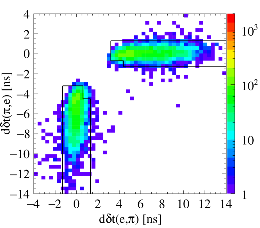
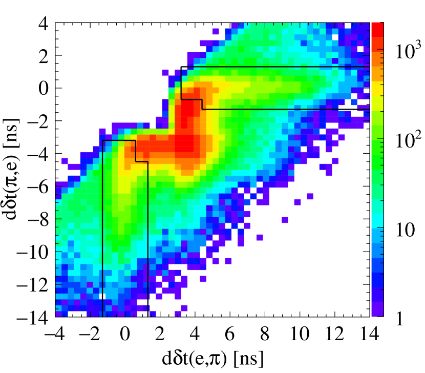
Figure 1: Distribution of ${\rm d}\delta(\pi,e)$ vs ${\rm d}\delta(e,\pi)$ for $\mathrm{K_{S}}\mathrm{K_{L}}\to(\pi^{\pm}e^{\mp}\nu)(3\pi^{0})$ MC-simulated events (left) and all data events (right). Solid lines denote accepted regions, each corresponding to one possible assignment of pion and electron mass hypotheses’ to the two DC tracks in an event.

After the pion and electron tracks are identified, a second cut is applied in the $\delta t(\pi)$ vs $\delta t(e)$ plane as shown in Fig. 2 to further discriminate the remaining $\pi^{+}\pi^{-}$ events. After these cuts, background remains (amounting to about 12% of the event sample) constituted by the $\mathrm{K_{S}}\to\pi^{0}\pi^{0}$ and $\mathrm{K_{L}}\to\pi e\nu$ processes where the $\mathrm{K_{S}}$ decay along with additional clusters had been misidentified as an early $\mathrm{K_{L}}\to 3\pi^{0}$ decay. This background is discriminated by removing events containing more than one cluster for which $R/(cT_{clu})>0.9$ where $R$ is the distance between the IP and the cluster (corresponding to photons emitted close to the IP).

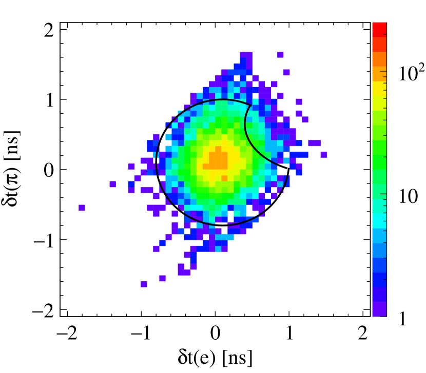
Figure 2: Distribution of $\delta t(\pi)$ vs $\delta t(e)$ after particle identification for MC-simulated $\mathrm{K_{S}}\mathrm{K_{L}}\to(\pi^{\pm}e^{\mp}\nu)(3\pi^{0})$ events (left) and all data events (right). Events inside the region marked with black solid line are accepted.

The remaining background (in the order of decreasing contribution) is composed of:

• $\mathrm{K_{S}}\to\pi^{+}\pi^{-}$ with imperfect track reconstruction,

• $\mathrm{K_{S}}\to\pi^{+}\pi^{-}\to\pi\mu\nu$ decay chain where one of the charged pions decays into a muon and a neutrino before entering the DC,

• radiative $\mathrm{K_{S}}\to\pi^{+}\pi^{-}\gamma$ decays dominated by inner bremsstrahlung [38, 39].

As all these events are characterised by a pion or muon track misidentified as $e^{+}/e^{-}$, two particle binary classifiers based on Artificial Neural Networks (ANNs) (using Multilayer Perceptron from the TMVA package [40]) and acting on an ensemble constituted by a track and its associated cluster are prepared for $e/\pi$ and $\mu/\pi$ discrimination in subsequent steps. Classification is based on the different structure of the energy deposited in the EMC cells by electrons, pions, and muons, in combination with the information of the particle momentum from the associated DC track. The ANNs are trained using data control samples of $\mathrm{K_{L}}\to\pi^{\pm}e^{\mp}\nu$ and $\mathrm{K_{L}}\to\pi^{\pm}\mu^{\mp}\nu$ decays tagged by $\mathrm{K_{S}}\to\pi^{+}\pi^{-}$ identified with a 98% purity according to MC simulations.

After the $e/\pi$ and $e/\mu$ particle discrimination for lepton track candidates, the signal to background ratio amounts to 22.5 with residual background dominated by $\mathrm{K_{S}}\to\pi^{+}\pi^{-}$ (55%), $\mathrm{K_{S}}\to\pi^{+}\pi^{-}\gamma$ (19%) and events with $\mathrm{K_{L}}$ decays other than $3\pi^{0}$ (12%). Distribution of the residual background as a function of $\Delta t$ is modelled with an exponential function presented in Fig. 3. Parameters of the exponential models are obtained with a fit to MC residual background separately for event samples with an electron and positron with $\chi^{2}$/NDF of 2.1 and 0.99 respectively. These models are used to subtract the expected background contamination from the data distributions shown in black points in Fig. 3.

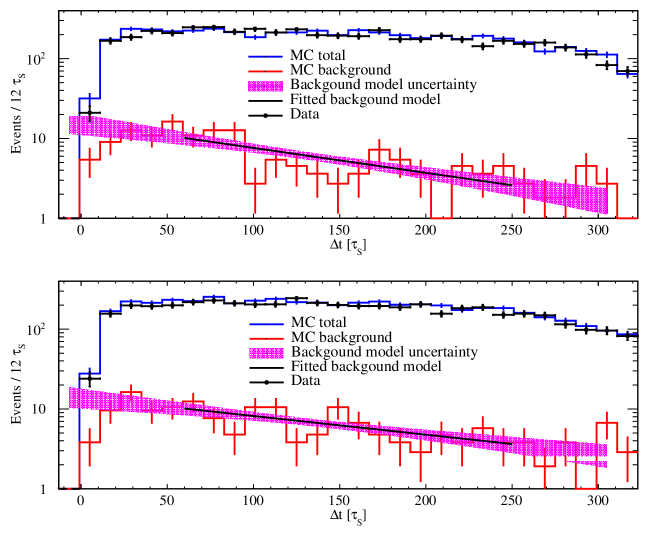
Figure 3: $\mathrm{K_{S}}\mathrm{K_{L}}\to(\pi^{\pm}e^{\mp}\nu)(3\pi^{0})$ sample: exponential model of residual background distribution as a function of $\Delta t$ for events with an electron (top) and positron (bottom) in the early kaon semileptonic decay. The modelled expected background is obtained in a fit to MC residual background and subtracted from the respective data distributions. Uncertainty of the fitted models (magenta band) is taken into account as a source of systematic uncertainty.

4.2 Selection of $\mathrm{K_{S}}\mathrm{K_{L}}\to(\pi^{+}\pi^{-})(\pi^{\pm}e^{\mp}\nu)$ events

As $\mathrm{K_{-}}\to\mathrm{K}^{0}$ and $\mathrm{K_{-}}\to\overline{\mathrm{K}}^{0}$ transitions are characterised by an early kaon decay into two pions (the $\pi^{+}\pi^{-}$ final state is chosen in this analysis) followed by a later semileptonic decay, event selection requires presence of a DC vertex associated to 2 opposite curvature tracks within a cylindrical volume of $\rho<15$ cm and $|z|<10$ cm around the IP and with $|m_{\pi\pi}-m_{\mathrm{K}^{0}}|<10$ MeV/c².

To find the semileptonic decay vertex, all vertices formed by two opposite curvature tracks in the DC are considered, excluding the previously identified $\mathrm{K_{S}}\to\pi^{+}\pi^{-}$ vertex and its related tracks. For each candidate semileptonic vertex the following invariant mass (which for correct $e/\pi$ identification should correspond to the electron mass) is evaluated separately for each track:

$$m^{2}_{\pm}=(E_{K}-E(\pi)_{\mp}-|\vec{p}_{miss}|)^{2}-|\vec{p}_{\pm}|^{2},$$ (22)

with $E_{K}$ being the energy of the decaying kaon, $E(\pi)_{\mp}$ the energy attributed to the track of negative (positive) charge assuming the charged pion mass, $\vec{p}_{\pm}$ the momentum corresponding to positive (negative) charge track, and $\vec{p}_{miss}=\vec{p}_{K}-\vec{p}_{+}-\vec{p}_{-}$. In the dominant background sources ($\pi^{+}\pi^{-}\pi^{0}$ and semileptonic decays with a muon) both tracks are characterised by significant $m^{2}$ values whereas for genuine $\pi^{\pm}e^{\mp}\nu$ decays $m^{2}\approx 0$ for one of the tracks, making the sum of $m^{2}$ for both tracks in the event sensitive to a difference between $\mathrm{K_{L}}\to\pi^{\pm}e^{\mp}\nu$ vertices and other decays as shown in Fig. 4. Vertex candidates with $m^{2}_{+}+m^{2}_{-}>0.015\>(\mathrm{GeV}/c^{2})^{2}$ are rejected and only events with one remaining vertex candidate are considered in further analysis.

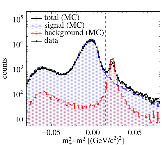
Figure 4: Sum of invariant masses of two decay product tracks assuming their electron mass hypotheses and a semileptonic decay. Background and data distributions contain contributions from different decay vertex choices. $\mathrm{K_{L}}$ decay vertex candidates with $m^{2}_{+}+m^{2}_{-}>0.015\>(\mathrm{GeV}/c^{2})^{2}$ (i.e. right of the dashed vertical line) are rejected.

Further selection of semileptonic decays of $\mathrm{K_{L}}$ as well as identification of the $e^{\pm}$ and $\pi^{\pm}$ tracks is performed with a time of flight analysis similarly as in the case of $\mathrm{K_{S}}\to\pi^{\pm}e^{\mp}\nu$, resulting in signal to background ratio of 75. The remaining background is neglected in further analysis.

4.3 Determination of efficiencies

For each of the two classes of processes, selected events are split by charge of the electron and positron from the semileptonic decay. $\Delta t$-dependent efficiencies are evaluated separately for each of the obtained four samples of events as:

$$\varepsilon_{total}(\Delta t)=\varepsilon_{TEC}\times\varepsilon_{SEL}(\Delta t),$$ (23)

where $\varepsilon_{TEC}$ is the combination of $\Delta t$-independent efficiencies of trigger, machine background filter and event classification described in Section 3 and $\varepsilon_{SEL}(\Delta t)$ represents the efficiency of event selection (cuts) for a particular $\Delta t$ interval.

For evaluation of the trigger efficiency, rates of events with either one – EMC or DC based – or both triggers for events passing the entire event selection, are used to obtain the total probability of at least one of the triggers present on a signal event. Efficiency of the machine background filter is estimated by counting events passing the signal selection criteria among 10% of all events acquired independently of the filter decision. Similarly, a subsample of 5% of all events stored independently of their classification is used to evaluate the probability of misclassification of a signal event and thus the classification efficiency. Table 1 summarises the $\varepsilon_{TEC}$ efficiencies combining these three factors for each class of signal events.

Table 1: Combined efficiencies of trigger, machine background filter and event classification for the four event samples.

event sample	$\varepsilon_{TEC}$ [%]
$(\pi^{+}e^{-}\nu)\;(3\pi^{0})$	99.487 $\pm$ 0.071
$(\pi^{-}e^{+}\nu)\;(3\pi^{0})$	99.453 $\pm$ 0.074
$(\pi^{+}\pi^{-})\;(\pi^{+}e^{-}\nu)$	99.597 $\pm$ 0.007
$(\pi^{+}\pi^{-})\;(\pi^{-}e^{+}\nu)$	99.589 $\pm$ 0.010

Event selection efficiencies are estimated using Monte Carlo simulations of the respective event classes. In case of semileptonic decays, MC-based efficiencies $\varepsilon_{SEL}(\Delta t)$ are corrected using an independent data control sample of $\mathrm{K_{S}}\mathrm{K_{L}}\to(\pi^{0}\pi^{0})(\pi^{\pm}e^{\mp}\nu)$ events. The selection efficiency for $\mathrm{K_{L}}\to 3\pi^{0}$ decays is estimated with MC and corrected with a $\mathrm{K_{S}}\mathrm{K_{L}}\to(\pi^{+}\pi^{-})(3\pi^{0})$ data control sample.

5 Ratios of double kaon decay rates

After event selection, the counts of events identified for each class are presented in Table 2. Fig. 5 shows a summary of the corresponding data $\Delta t$ distributions entering the probability ratios along with their respective $\varepsilon_{SEL}(\Delta t)$ event selection efficiencies in the range $0<\Delta t<320\>\tau_{S}$, with a bin width of $12\>\tau_{S}$.

Table 2: Numbers of events identified for each of the four event classes.

event sample	events
$(\pi^{+}e^{-}\nu)\;(3\pi^{0})$	4750
$(\pi^{-}e^{+}\nu)\;(3\pi^{0})$	4652
$(\pi^{+}\pi^{-})\;(\pi^{+}e^{-}\nu)$	15924863
$(\pi^{+}\pi^{-})\;(\pi^{-}e^{+}\nu)$	15708190

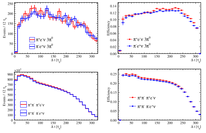
Figure 5: Left column: Rates of double kaon decays as a function of $\Delta t$ for the two studied classes of processes and two lepton charge subsamples. Right column: corresponding $\varepsilon_{SEL}(\Delta t)$ efficiencies.

The T and CPT-violation sensitive single ratios defined in Eqs. (7) and (9) are shown in Figs. 6 and 7. Each point of the single ratio graphs is defined through the counts of the respective double kaon decays $N_{i}$ and $N^{\prime}_{i}$ in the $i$-th interval of $\Delta t$ and their corresponding event identification efficiencies $\varepsilon_{i}$ and $\varepsilon^{\prime}_{i}$ as:

$$R_{i}\equiv R(\Delta t_{i})=\frac{N_{i}}{N_{i}^{\prime}}\frac{\varepsilon_{i}^{\prime}}{\varepsilon_{i}}\frac{1}{D},$$ (24)

where $D$ is the factor defined in Section 1.

Figure 6: T-violation sensitive ratios of double decay rates as defined in Eq. (7). Dashed lines denote levels obtained with the fit.

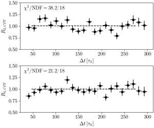
Figure 7: CPT-violation sensitive ratios of double decay rates as defined in Eq. (9). Dashed lines denote levels obtained with the fit.

Due to the limited statistics of the process entering the numerator of the ratios, a constant level of the single ratios is evaluated in the range of high and relatively stable efficiency of $\Delta t\in(47,275)\tau_{S}$ using a maximum likelihood fit for the constant ratio $R_{\SS}$:

$$\mathcal{L}(R_{\SS})=\prod_{i\text{ in fit limits}}p\left(N_{i},\>R_{\SS}N_{i}^{\prime}D\frac{\varepsilon_{i}}{\varepsilon_{i}^{\prime}}\right),$$ (25)

where $p(n,\>\lambda)$ is the Poissonian probability of observing $n$ counts with the distribution mean of $\lambda$.

Counts of the $(\pi^{+}\pi^{-})(\pi^{\pm}e^{\mp}\nu)$ events with a positron and an electron are also used to construct transition rate ratios sensitive to CP-violation (Eq. (8)) shown in Fig. 8. Finally, double ratios sensitive to T and CP violation (Eq. (19)) and CPT violation (Eq. (20)) are constructed and their asymptotic levels are estimated as presented in Fig. 9.

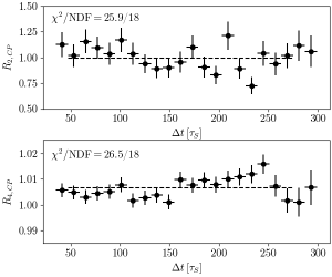
Figure 8: Ratios of the rates of $(\pi^{\pm}e^{\mp}\nu)(3\pi^{0})$ (top) and $(\pi^{+}\pi^{-})(\pi^{\pm}e^{\mp}\nu)$ (bottom) events sensitive to CP-violation effects. Dashed lines denote levels obtained with the fit.

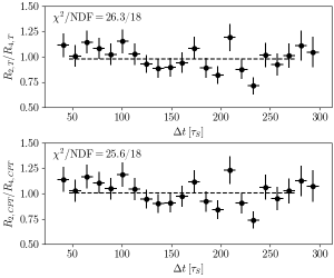
Figure 9: Double ratios of double kaon decay rates sensitive to effects of T and CP violation (top) and CPT violation (bottom). Dashed lines denote levels obtained with the fit.

6 Systematic uncertainties

Stability of the results is checked by varying the event selection cut values by $\pm 5\sigma$ in steps of $1~{}\sigma$ where $\sigma$ denotes the resolution on the variable subject to the cut, repeating the analysis for each cut value and observing the impact of variation on each of the eight observables of the tests. For evaluation of the corresponding systematic uncertainties absolute deviations of each of the observables for $\pm 1\sigma$ cut variation are averaged.

The uncertainty due to the model of subtracted background is estimated by varying the two model parameters within their errors. Effects from $\pm 1\sigma$ variations of each parameter of the model are added in quadrature.

Event selection efficiencies based on MC simulations with limited statistics are subject to a smoothing procedure. The corresponding systematic uncertainty is quantified by comparing analysis results with and without efficiency smoothing.

The choice of $\Delta t$ bin width for the final ratio distributions and the fit limits account for another source of systematic uncertainty. Stability of the fit results is tested for bin widths ranging from 3 $\tau_{S}$ to 24 $\tau_{S}$ and an average of the observables’ deviations obtained with the extreme bin widths from the result with 12 $\tau_{S}$ is used as an estimate of the systematic effect. The fitting range is varied by $\pm 24\ \tau_{S}$ in steps of $\pm 6\ \tau_{S}$ as a shift as well as total width. Changes of the fitted ratio levels for variations of $\pm 6\ \tau_{S}$ are averaged and added in quadrature.

Table 3 summarises all identified systematic effects on each of the eight observables of the tests. All contributions are added in quadrature to obtain the total systematic uncertainties indicated in bold. In case of single ratios, the results are additionally affected by the total error on the $D$ factor (quoted separately due to containing both statistical and systematic contributions) obtained from previous KLOE measurements.

Table 3: Systematic uncertainties on all of the symmetry test observables. In case of $R_{2,CP}$ and $R_{4,CP}$, each ratio is obtained using only one class of events and thus not affected by effects of selection of the other class. The uncertainty of the D factor comprises both statistical and systematic errors.

Effect	$R_{2,T}$	$R_{4,T}$	$R_{2,{CPT}}$	$R_{4,{CPT}}$	$DR_{T,CP}$	$DR_{CPT}$	$R_{2,CP}$	$R_{4,CP}$
	$\times\ 10^{-3}$	$\times\ 10^{-3}$	$\times\ 10^{-3}$	$\times\ 10^{-3}$	$\times\ 10^{-3}$	$\times\ 10^{-3}$	$\times\ 10^{-3}$	$\times\ 10^{-3}$
Background model	2.74	4.62	2.79	4.43	4.43	4.41	4.37	–
Efficiency smoothing	2.46	5.31	2.43	5.26	6.70	6.83	6.76	0.17
$\Delta t$ bin width	8.00	5.00	7.50	5.50	9.00	9.00	8.90	0.03
Fit range	7.33	8.88	7.32	8.84	7.95	7.60	7.78	0.41
Effects of cuts in the $(\pi e\nu)(3\pi^{0})$ selection
$\mathrm{K_{S}}$ vertex location cuts	0.57	2.31	0.58	2.27	2.36	2.41	2.39	–
M($\pi,\pi$) cut	2.48	1.34	2.52	1.31	1.56	1.63	1.60	–
TOF cuts	6.08	5.32	6.19	5.23	6.40	6.58	6.49	–
e/$\pi$/$\mu$ classification	4.78	4.40	4.85	4.33	9.33	9.59	9.46	–
Effects of cuts in the $(\pi^{+}\pi^{-})(\pi e\nu)$ selection
$\mathrm{K_{S}}$ vertex location cuts	0.007	0.004	0.004	0.007	0.004	0.004	–	0.005
M($\pi,\pi$) and $|\vec{p}|$ cuts	2.14	1.68	1.67	2.17	0.70	0.72	–	0.74
$m^{2}_{+}+m^{2}_{-}$ cut	1.48	1.32	1.31	1.49	0.20	0.21	–	0.21
TOF cuts	2.14	1.68	1.67	2.17	0.70	0.72	–	0.74
Total systematic uncertainty	14	15	14	15	19	19	19	0.89
D factor total uncertainty	12	12	12	12	–	–	–	–

7 Results and conclusions

We presented the first direct tests of $\mathrm{T}$, $\mathrm{CP}$, $\mathrm{CPT}$ symmetries in transitions of neutral kaons, obtained analysing $1.7~{}\hbox{fb}^{-1}$ of data collected by the KLOE experiment at DA$\Phi$NE. The $\mathrm{T}$ and $\mathrm{CPT}$ tests involving time-reversal implement the necessary exchange of in and out states, as required for a genuine test, exploiting the entanglement of the $\mathrm{K^{0}}\mathrm{\overline{K}{}^{0}}$ pairs. The decay intensities of the processes $\phi\rightarrow\mathrm{K_{S}}\mathrm{K_{L}}\rightarrow\pi^{+}\pi^{-}\,\pi e\nu$ and $\phi\rightarrow\mathrm{K_{S}}\mathrm{K_{L}}\rightarrow\pi e\nu\,3\pi^{0}$ as a function of $\Delta t$ are measured in the asymptotic region $\Delta t\gg\tau_{S}$, statistically the most significant. We get results for all eight observables defined in Eqs. (13)–(20):

$$R_{2,T}= 0.991 \pm 0.017_{stat}\pm 0.014_{syst}\pm{0.012}_{D},$$

$$R_{4,T}= 1.015 \pm 0.018_{stat}\pm 0.015_{syst}\pm{0.012}_{D},$$

$$R_{2,{CPT}}= 1.004 \pm 0.017_{stat}\pm 0.014_{syst}\pm{0.012}_{D},$$

$$R_{4,{CPT}}= 1.002 \pm 0.017_{stat}\pm 0.015_{syst}\pm{0.012}_{D},$$

$$R_{2,{CP}}= 0.992 \pm 0.028_{stat}\pm 0.019_{syst},$$

$$R_{4,{CP}}= 1.00665 \pm 0.00093_{stat}\pm 0.00089_{syst},$$

$$DR_{T,CP}=R_{2,{T}}/R_{4,{T}}= 0.979 \pm 0.028_{stat}\pm 0.019_{syst},$$

$$DR_{CPT}=R_{2,{CPT}}/R_{4,CPT}= 1.005 \pm 0.029_{stat}\pm 0.019_{syst}.$$

A comparison of these results with expected values (assuming $\mathrm{CPT}$ invariance and $\mathrm{T}$ violation extrapolated from observed $\mathrm{CP}$ violation in the mixing) is presented in Fig. 10.

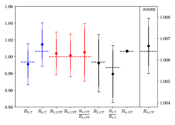
Figure 10: Comparison of the measured symmetry-violation-sensitive single and double ratios and their expected values (horizontal dashed lines) assuming $\mathrm{CPT}$ invariance and $\mathrm{T}$ violation extrapolated from observed $\mathrm{CP}$ violation in the mixing. Solid error bars denote statistical uncertainties and dotted error bars represent total uncertainties (including error on the D factor in case of single $\mathrm{T}$ and $\mathrm{CPT}$-violation sensitive ratios). The right-hand-side panel magnifies the region of the $\mathrm{CP}$-violation-sensitive ratio $R_{4,CP}.$

For the $\mathrm{T}$ and $\mathrm{CPT}$ single ratios a total relative error of $2.5~{}\%$ is reached, while for the double ratios (19) and (20) the total error increases to $3.5~{}\%$, with the advantage of improved sensitivity to violation effects, and of independence from the $D$ factor. The measurement of the single ratio $R_{4,\mathrm{CP}}$ benefits of highly allowed decay rates for the involved channels, reaching an error of $0.13~{}\%$.

The double ratio $DR_{\mathrm{CPT}}$ is our best observable for testing $\mathrm{CPT}$, free from approximations and model independent, while $DR_{\mathrm{T},\mathrm{CP}}$ assumes no direct $\mathrm{CPT}$ violation and is even under $\mathrm{CPT}$, therefore it does not disentangle $\mathrm{T}$ and $\mathrm{CP}$ violation effects, contrary to the genuine $\mathrm{T}$ and $\mathrm{CP}$ single ratios.

No result on $\mathrm{T}$ and $\mathrm{CPT}$ observables shows evidence of symmetry violation. We observe $\mathrm{CP}$ violation in transitions in the single ratio $R_{4,\mathrm{CP}}$ with a significance of $5.2\sigma$, in agreement with the known $\mathrm{CP}$ violation in the $\mathrm{K^{0}}-\mathrm{\overline{K}{}^{0}}$ mixing using a different observable.

References

- [1] E. P. Wigner, Gruppentheorie und ihre Anwendung auf die Quanten Mechanik der Atomspektren, Vieweg, Braunschweig Germany, 1931.
- [2] L. Wolfenstein, The search for direct evidence for time reversal violation, Int. J. Mod. Phys. E 8 (1999) 501–511. doi:10.1142/S0218301399000343.
- [3] L. Wolfenstein, Violation Of Time Reversal Invariance in K0 Decays, Phys. Rev. Lett. 83 (1999) 911–912. doi:10.1103/PhysRevLett.83.911.
- [4] M. C. Banuls, J. Bernabéu, CP, T and CPT versus temporal asymmetries for entangled states of the Bd-system, Phys. Lett. B 464 (1999) 117–122. arXiv:hep-ph/9908353, doi:10.1016/S0370-2693(99)01043-6.
- [5] M. C. Banuls, J. Bernabéu, Studying indirect violation of CP, T and CPT in a B-factory, Nucl. Phys. B 590 (2000) 19–36. arXiv:hep-ph/0005323, doi:10.1016/S0550-3213(00)00548-4.
- [6] J. Bernabéu, F. Martinez-Vidal, P. Villanueva-Perez, Time Reversal Violation from the entangled 0 system, JHEP 08 (2012) 064. arXiv:1203.0171, doi:10.1007/JHEP08(2012)064.
- [7] J. P. Lees, et al., Observation of Time Reversal Violation in the Meson System, Phys. Rev. Lett. 109 (2012) 211801. arXiv:1207.5832, doi:10.1103/PhysRevLett.109.211801.
- [8] E. Applebaum, A. Efrati, Y. Grossman, Y. Nir, Y. Soreq, Subtleties in the measurement of time-reversal violation, Phys. Rev. D 89 (2014) 076011. arXiv:1312.4164, doi:10.1103/PhysRevD.89.076011.
- [9] J. Bernabéu, F. J. Botella, M. Nebot, Genuine T, CP, CPT asymmetry parameters for the entangled Bd system, JHEP 06 (2016) 100. arXiv:1605.03925, doi:10.1007/JHEP06(2016)100.
- [10] J. Bernabéu, A. Di Domenico, P. Villanueva-Perez, Direct test of time-reversal symmetry in the entangled neutral kaon system at a -factory, Nucl. Phys. B 868 (2013) 102–119. arXiv:1208.0773, doi:10.1016/j.nuclphysb.2012.11.009.
- [11] J. Bernabéu, A. Di Domenico, P. Villanueva-Perez, Probing CPT in transitions with entangled neutral kaons, JHEP 10 (2015) 139. arXiv:1509.02000, doi:10.1007/JHEP10(2015)139.
- [12] A. Angelopoulos, et al., First direct observation of time reversal noninvariance in the neutral kaon system, Phys. Lett. B 444 (1998) 43–51. doi:10.1016/S0370-2693(98)01356-2.
- [13] J. Bernabéu, F. Martinez-Vidal, Colloquium: Time-reversal violation with quantum-entangled B mesons, Rev. Mod. Phys. 87 (2015) 165. arXiv:1410.1742, doi:10.1103/RevModPhys.87.165.
- [14] A. Angelopoulos, et al., A Determination of the CPT violation parameter Re() from the semileptonic decay of strangeness tagged neutral kaons, Phys. Lett. B 444 (1998) 52–60. doi:10.1016/S0370-2693(98)01357-4.
- [15] G. Luders, Proof of the TCP theorem, Annals Phys. 2 (1957) 1–15. doi:10.1016/0003-4916(57)90032-5.
- [16] W. Pauli, Exclusion Principle, Lorentz Group and Reflection of Space-Time and Charge, Pergamon, London, UK, 1955, pp. 30–51.
- [17] J. S. Bell, Time reversal in field theory, Proc. Roy. Soc. Lond. A 231 (1955) 479–495. doi:10.1098/rspa.1955.0189.
- [18] R. Jost, Eine Bemerkung zum CPT-theorem, Helv. Phys. Acta 30 (1957) 409–416.
- [19] D. Babusci, et al., Precision tests of quantum mechanics and symmetry with entangled neutral kaons at KLOE, JHEP 04 (2022) 059. arXiv:2111.04328, doi:10.1007/JHEP04(2022)059.
- [20] J. Bernabéu, A. Di Domenico, Can future observation of the living partner post-tag the past decayed state in entangled neutral K mesons?, Phys. Rev. D 105 (11) (2022) 116004. arXiv:1912.04798, doi:10.1103/PhysRevD.105.116004.
- [21] C. O. Dib, B. Guberina, Almost forbidden Delta Q = - Delta S processes, Phys. Lett. B 255 (1991) 113–116. doi:10.1016/0370-2693(91)91149-P.
- [22] A. Di Domenico, Testing Discrete Symmetries in Transitions with Entangled Neutral Kaons, Acta Phys. Polon. B 48 (2017) 1919. doi:10.5506/APhysPolB.48.1919.
-
[23]
INFN,
Handbook
on neutral kaon interferometry at a -factory, Vol. 43 of Frascati
physics series, INFN, Frascati, Italy, 2007.
URL http://www.lnf.infn.it/sis/frascatiseries/Volume43/volume43.pdf - [24] F. Ambrosino, et al., Measurement of the KL meson lifetime with the KLOE detector, Phys. Lett. B 626 (2005) 15–23. arXiv:hep-ex/0507088, doi:10.1016/j.physletb.2005.08.022.
- [25] F. Ambrosino, et al., Measurements of the absolute branching ratios for the dominant KL decays, the KL lifetime, and Vus with the KLOE detector, Phys. Lett. B 632 (2006) 43–50. arXiv:hep-ex/0508027, doi:10.1016/j.physletb.2005.10.018.
- [26] F. Ambrosino, et al., Precise measurement of ) with the KLOE detector at DANE, Eur. Phys. J. C 48 (2006) 767–780. arXiv:hep-ex/0601025, doi:10.1140/epjc/s10052-006-0021-9.
- [27] F. Ambrosino, et al., Precision measurement of meson lifetime with the KLOE detector, Eur. Phys. J. C 71 (2011) 1604. arXiv:1011.2668, doi:10.1140/epjc/s10052-011-1604-7.
- [28] P. Zyla, et al., Review of Particle Physics, PTEP 2020 (8) (2020) 083C01. doi:10.1093/ptep/ptaa104.
- [29] A. Di Domenico, Entanglement, CPT and neutral kaons, in: Proceedings of the 9th Meeting on CPT and Lorentz Symmetry, Bloomington, Indiana, USA, May 17-26, 2022. arXiv:2208.06789.
- [30] V. Weisskopf, E. Wigner, Over the natural line width in radiation of the harmonius oscillator, Z. Phys. 65 (1930) 18.
- [31] A. Gallo, et al., DAFNE status report, Conf. Proc. C 060626 (2006) 604–606.
- [32] M. Adinolfi, F. Ambrosino, A. Andryakov, A. Antonelli, M. Antonelli, et al., The tracking detector of the KLOE experiment, Nucl. Instrum. Meth. A 488 (2002) 51–73. doi:10.1016/S0168-9002(02)00514-4.
- [33] M. Adinolfi, F. Ambrosino, A. Antonelli, M. Antonelli, F. Anulli, et al., The KLOE electromagnetic calorimeter, Nucl. Instrum. Meth. A 482 (2002) 364–386. doi:10.1016/S0168-9002(01)01502-9.
- [34] M. Adinolfi, et al., The QCAL tile calorimeter of KLOE, Nucl. Instrum. Meth. A 483 (2002) 649–659. doi:10.1016/S0168-9002(01)01929-5.
- [35] M. Adinolfi, et al., The trigger system of the KLOE experiment, Nucl. Instrum. Meth. A 492 (2002) 134–146. doi:10.1016/S0168-9002(02)01313-X.
- [36] F. Ambrosino, et al., Data handling, reconstruction, and simulation for the KLOE experiment, Nucl. Instrum. Meth. A 534 (2004) 403–433. arXiv:physics/0404100, doi:10.1016/j.nima.2004.06.155.
-
[37]
A. Gajos,
Investigations
of fundamental symmetries with the electron-positron systems, Ph.D. thesis,
Jagiellonian University, Kraków, Poland (2018).
arXiv:1805.06009.
URL http://koza.if.uj.edu.pl/files/40f2a1011572dd7e0c9988c54dcaecaa/1805.06009.pdf - [38] E. Ramberg, et al., Simultaneous Measurement of and Decays into , Phys. Rev. Lett. 70 (1993) 2525–2528. doi:10.1103/PhysRevLett.70.2525.
- [39] C. Gatti, Monte Carlo simulation for radiative kaon decays, Eur. Phys. J. C 45 (2006) 417–420. arXiv:hep-ph/0507280, doi:10.1140/epjc/s2005-02435-2.
- [40] A. Hocker, et al., TMVA - Toolkit for Multivariate Data Analysis (3 2007). arXiv:physics/0703039.
-
[41]
M. Zobov, D. Alesini, M. E. Biagini, C. Biscari, A. Bocci, et al.,
Test of
“crab-waist” collisions at the
factory, Phys. Rev. Lett. 104 (2010) 174801.
doi:10.1103/PhysRevLett.104.174801.
URL https://link.aps.org/doi/10.1103/PhysRevLett.104.174801 - [42] C. Milardi, M. A. Preger, P. Raimondi, F. Sgamma, High luminosity interaction region design for collisions inside high field detector solenoid, JINST 7 (2012) T03002. arXiv:1110.3212, doi:10.1088/1748-0221/7/03/T03002.