An Intraday GARCH Model for Discrete Price Changes
and Irregularly Spaced Observations

Abstract: We develop a novel observation-driven model for high-frequency prices. We account for irregularly spaced observations, simultaneous transactions, discreteness of prices, and market microstructure noise. The relation between trade durations and price volatility, as well as intraday patterns of trade durations and price volatility, is captured using smoothing splines. The dynamic model is based on the zero-inflated Skellam distribution with time-varying volatility in a score-driven framework. Market microstructure noise is filtered by including a moving average component. The model is estimated by the maximum likelihood method. In an empirical study of the IBM stock, we demonstrate that the model provides a good fit to the data. Besides modeling intraday volatility, it can also be used to measure daily realized volatility.

Keywords: Ultra-High-Frequency Data, Trade Duration, Price Volatility, UHF-GARCH Model, Score-Driven Model, Skellam Distribution.

JEL Codes: C22, C41, C58, G12.

1 Introduction

Modeling intraday volatility presents several challenges in contrast to modeling volatility at the daily level as high-frequency data have distinct characteristics. A widely used tool for modeling daily volatility is the class of generalized autoregressive conditional heteroskedasticity (GARCH) models with seminal contributions by Engle (1982), Bollerslev (1986, 1987), and Nelson (1991). A variety of intraday GARCH models extending daily models therefore emerged, following the call for research in this direction by Engle (2002). In this paper, we focus on the following four characteristics of high-frequency prices in the context of intraday GARCH models:

Irregularly spaced observations. Engle (2000) coined the term ultra-high-frequency (UHF) data, which refer to records of every transaction made resulting in irregularly spaced observations. Such data require special treatment in econometric modeling. Engle and Russell (1998) proposed to model times between successive transactions, also known as trade durations, by the autoregressive conditional duration (ACD) model. Furthermore, Engle (2000) proposed to model the variance per time unit using irregularly spaced observations by the UHF-GARCH model. Ghysels and Jasiak (1998) proposed an alternative GARCH model for UHF data in which the total variance is modeled but the GARCH parameters are functions of the expected duration. Meddahi et al. (2006) highlighted the differences between these two models. The UHF-GARCH model of Engle (2000) was further applied e.g. by Racicot et al. (2008) and Huptas (2016).

Simultaneous transactions. A particular issue of UHF data is the occurence of transactions with the same timestamp resulting in zero durations. Engle and Russell (1998) considered these transactions to be split transactions which belong to a single trade and decided to aggregate them. Note that zero duration does not necessarily mean zero return as transactions can be executed at the same time at different prices. Blasques et al. (2022a) further studied the issue of zero durations and pointed out that, depending on the precision of timestamps in data, zero durations may account for the majority of observations and aggregation is not a suitable solution. When measuring price variance per time unit, as Engle (2000) did, returns are divided by the square root of the corresponding trade duration. Zero durations with nonzero returns of course disrupt this concept of variance per time unit.

Discretness of prices. Financial assets are traded on a discrete grid of prices. On the NYSE and NASDAQ exchanges, e.g., stocks are traded with precision to one cent. This discreteness has a large impact on the distribution of returns (see, e.g., Münnix et al., 2010 for empirical evidence). Consequently, a strand of literature emerged that focuses on dynamic volatility models for discrete price changes based on the Skellam distribution and its generalizations. Koopman et al. (2017) modified the Skellam distribution by transferring probability mass between 0, 1, and -1 values and used it in a dynamic state space model for price changes. Koopman et al. (2018) took a multidimensional approach and modeled price changes by a score-driven model based on a discrete copula with Skellam margins. Alomani et al. (2018) used the Skellam GARCH model for drug crimes. Gonçalves and Mendes-Lopes (2020) studied more general integer GARCH processes with applications to polio cases and Olympic medals won. Cui et al. (2021) used a GARCH model based on the Skellam distribution with modified probabilities for daily price changes. Doukhan et al. (2021) studied theoretical properties of integer GARCH processes. Catania et al. (2022) used the zero-inflated Skellam distribution in a hidden Markov model for multivariate price changes. Note that none of these studies utilize UHF data and are limited only to a fixed frequency – e.g., 1 second in Koopman et al. (2017), 10 second in Koopman et al. (2018), and 15 second in Catania et al. (2022). In contrast to time series models, Skellam models in continuous time were analyzed by Barndorff-Nielsen et al. (2012) and Shephard and Yang (2017). An alternative approach was adopted by Holý and Tomanová (2022) who modeled prices directly, instead of price changes or logarithmic returns, by the double Poisson distribution.

Market microstructure noise. A well documented feature of high frequency data is market microstructure noise – a deviation from the fundamental efficient price (see, e.g., Hansen and Lunde, 2006 for an in-depth study). It is caused by price discreteness but also by bid-ask bounce, asymmetric information of traders, and other informational effects. It plays a key role in nonparametric estimation of quadratic variation and integrated variance as it significantly biases realized variance at higher frequencies (see, e.g., Holý and Tomanová, 2023 for an overview of noise-robust estimators). Regarding parametric processes, independent market microstructure noise induces a moving average component of order one. Specifically, Aït-Sahalia et al. (2005) showed that Wiener process contaminated by independent market microstructure noise sampled at discrete times corresponds to ARIMA(0,1,1) process and Holý and Tomanová (2019) showed that discretized noisy Ornstein–Uhlenbeck process corresponds to ARIMA(1,0,1) process.

Table 1 lists notable high-frequency models and summarizes their features. Note that none of these models address all four of the above high-frequency characteristics. The goal of this paper is therefore to combine the UHF-GARCH approach with the Skellam-GARCH approach while accounting for simultaneous transactions and market microstructure noise.

Our approach starts with nonparametric estimation of diurnal trends in trade durations and squared price changes using smoothing splines. When both these time series are adjusted for diurnal trends, their relation is estimated using smoothing splines. Next, we build our dynamic model. The original (unadjusted) price changes are assumed to follow the zero-inflated Skellam distribution of Skellam (1946) with time-varying mean and variance and static probability of zero-inflation. The dynamic mean follows MA(1) process to capture the effects of market microstructure noise. As high-frequency data exhibit zero expected returns, we set the intercept to zero. In the Skellam distribution, the variance is required to be higher than the absolute value of the mean, which is suitable for high-frequency data. However, to avoid inconvenient restrictions on the parameter space, we propose to parametrize the distribution in terms of the overdispersion parameter, i.e. the excessive variance. The dynamic overdispersion then follows score-driven model, developed by Creal et al. (2013) and Harvey (2013). The estimated diurnal pattern of squared price changes and their relation to trade durations are further plugged into this dynamics. The used relation to trade durations simultaneously captures adjustment of variance to time unit and the residual dependency on trade durations, which were modeled separately by Engle (2000). The proposed joint modeling removes the problems with zero trade durations, which can be quite frequent in high-frequency data. The proposed model belongs to the class of observation-driven models and can be estimated by the maximum likelihood method, which makes it suitable even for large datasets.

In an empirical study, we focus on the IBM stock (just as, e.g., Engle and Russell, 1998; Engle, 2000) from March to July, 2022. However, we also report results for 6 other stocks traded on the NYSE and NASDAQ exchanges. We estimate intraday models with various specifications for each of the 105 trading days in our dataset. For the IBM stock, the average number of observations in a day is 63 673. We show that the proposed model is a good fit and all its components are justifiable. We also demonstrate how the results can be used as an alternative to daily realized measures of volatility such as the realized kernel of Barndorff-Nielsen et al. (2008). Finally, we find that the relation between price volatility and trade durations is the same as described by Engle (2000), eventhough the magnitude of high-frequency data has increased considerabely since then.

Table 1: An overview of selected high-frequency time series models and their features – using ultra-high-frequency data with irregularly spaced observations (Irreg), accounting for simultaneous transactions with zero trade durations (Simul), accounting for discrete prices or price changes (Discrete), accounting for market microstructure noise (Noise), joint modeling of volatility and trade durations (Duration), joint modeling of volatility and trade volume (Volume), and multivariate modeling (Multi).

Paper	Irreg	Simul	Discrete	Noise	Duration	Volume	Multi
Ghysels and Jasiak (1998)	✓	✗	✗	✗	✓	✗	✗
Engle (2000)	✓	✗	✗	✗	✓	✗	✗
Grammig and Wellner (2002)	✓	✗	✗	✗	✓	✗	✗
Manganelli (2005)	✓	✗	✗	✗	✓	✓	✗
Russell and Engle (2005)	✓	✗	✓	✗	✓	✗	✗
Liu and Maheu (2012)	✓	✗	✗	✓	✓	✗	✗
Huptas (2016)	✓	✗	✗	✗	✓	✗	✗
Koopman et al. (2017)	✗	✗	✓	✗	✗	✗	✗
Koopman et al. (2018)	✗	✗	✓	✗	✗	✗	✓
Buccheri et al. (2021)	✗	✗	✗	✓	✗	✗	✓
Catania et al. (2022)	✗	✗	✓	✗	✗	✗	✓
Holý and Tomanová (2022)	✓	✗	✓	✗	✗	✗	✗
This study	✓	✓	✓	✓	✗	✗	✗

2 Methodology

2.1 Nonparametric Temporal Adjustment

Let $t_{i}$, $i=0,\ldots,n$, denote times of transactions and $p_{i}$, $i=0,\ldots,n$, prices (with precision to two decimal places). Furthermore, let $d_{i}=t_{i}-t_{i-1}$, $i=1,\ldots,n$, denote trade durations and $y_{i}=100(p_{i}-p_{i-1})$, $i=1,\ldots,n$, (integer) price changes.

First, we estimate the intraday pattern of trade durations. On each day, we standardize trade durations as $\bar{d}_{i}=d_{i}/\frac{1}{n}\sum_{i=1}^{n}d_{i}$. Using the complete dataset, we then estimate the (possibly nonlinear) dependence of $\bar{d}_{i}$ on $t_{i}$ by the cubic smoothing spline method (see, e.g., Hastie et al., 2008, Section 5.4). The chosen nonparametric method, however, is not essential to our model and alternatives can be used as well. We obtain the fitted function $\hat{f}_{\mathrm{dur}}(t_{i})$ and adjust trade durations as $\tilde{d}_{i}=\bar{d}_{i}/\hat{f}_{\mathrm{dur}}(t_{i})$.

Next, we estimate the intraday pattern of squared price changes. To be precise, squared price changes with substracted price changes in absolute value, $z_{i}=y_{i}^{2}-\lvert y_{i}\rvert=y_{i}(y_{i}-\mathrm{sgn}(y_{i}))$. This transformation corresponds to the overdispersion parameter, which plays a central role in our dynamic model. As in the case of trade durations, we standardize modified squared price changes as $\bar{z}_{i}=z_{i}/\frac{1}{n}\sum_{i=1}^{n}z_{i}$ and then estimate the dependence of $\bar{z}_{i}$ on $t_{i}$ by the cubic smoothing spline method. We obtain the fitted function $\hat{f}_{\mathrm{disp}}(t_{i})$ and adjust modified squared returns as $\tilde{z}_{i}=z_{i}/\hat{f}_{\mathrm{disp}}(t_{i})$.

Finally, we estimate the relation between modified squared price changes and trade durations, i.e. dependence of $\tilde{z}_{i}$ on $\tilde{d}_{i}$. Again, we use the cubic smoothing spline method and obtain the fitted function $\hat{f}_{\mathrm{rel}}(\tilde{d}_{i})$.

2.2 Zero-Inflated Skellam Distribution

The probability theory and statistics literature does not offer many distributions defined on integer support (without the nonnegativity or positivity constraint). The most used representative is the Skellam distribution of Skellam (1946), which is the distribution of the difference between two independent variables following the Poisson distribution with rates $\lambda_{1}$ and $\lambda_{2}$ respectively. Regarding dynamic models, it can be used when a time series of counts is nonstationary, but its first difference is stationary – a typical feature of high-frequency prices.

The Skellam distribution is often parametrized in terms of mean $\mu=\lambda_{1}-\lambda_{2}$ and variance $\sigma^{2}=\lambda_{1}+\lambda_{2}$ rather than rates $\lambda_{1}$ and $\lambda_{2}$ (see, e.g., Koopman et al., 2017, 2018; Alomani et al., 2018). However, in this parametrization, it is required that $\sigma^{2}>\lvert\mu\rvert$. When $\mu$ is nonzero, this condition can be hard to satisfy in dynamic models. For this reason, we propose an alternative parametrization with overdispersion parameter $\delta=\sigma^{2}-\lvert\mu\rvert=\min\{2\lambda_{1},2\lambda_{2}\}>0$ representing excessive variance.

In any case, only two parameters of the distribution do not offer much flexibility needed for high frequency prices. Koopman et al. (2017) deflate the probability of 0 and inflate probability of 1 and -1 using an additional parameter. On the other hand, Karlis and Ntzoufras (2006, 2009) and Catania et al. (2022) inflate the probability of 0 and deflate the probabilities of all other values using an additional parameter, in the fashion of the zero-inflated model of Lambert (1992). As our data exhibit increased occurence of zero values (in comparison to the fitted Skellam distribution), we follow the latter approach and introduce the zero-inflation parameter $\pi$ to the distribution.

The probability mass function of the zero-inflated Skellam distribution with the mean-overdispersion parametrization is given by

$$\mathrm{P}[Y=y\mid\mu,\delta,\pi]=\begin{cases}\pi+(1-\pi)\exp(-\lvert\mu\rvert-\delta)I_{0}\left(\sqrt{\delta^{2}+2\lvert\mu\rvert\delta}\right)&\text{ for }y=0,\\ (1-\pi)\exp(-\lvert\mu\rvert-\delta)\left(\frac{\lvert\mu\rvert+\mu+\delta}{\lvert\mu\rvert-\mu+\delta}\right)^{\frac{y}{2}}I_{y}\left(\sqrt{\delta^{2}+2\lvert\mu\rvert\delta}\right)&\text{ for }y\neq 0,\\ \end{cases}$$ (1)

where $I_{\cdot}(\cdot)$ is the modified Bessel function of the first kind. The first two moments are given by

$$\mathrm{E}[Y]=(1-\pi)\mu,\qquad\mathrm{var}[Y]=(1-\pi)\left(\lvert\mu\rvert+\delta+\pi\mu^{2}\right).$$ (2)

2.3 Time-Varying Parameters

In the dynamic model, we let the mean parameter $\mu$ and the overdispersion parameter $\delta$ be time-varying but keep the zero-inflation parameter $\pi$ static.

Strong negative first order autocorrelation, insignificant autocorrelation of higher order, and decaying negative partial autocorrealtion is typical for ultra-high-frequency price changes or returns and is caused by market microstrucure noise (see, e.g., Aït-Sahalia et al., 2005; Hansen and Lunde, 2006). It can be effectively captured by MA(1) process. Another typical feature of high-frequency data is zero mean of price changes or returns in long term (see, e.g., Koopman et al., 2017). We therefore model dynamics of the mean parameter as MA(1) process with zero intercept,

$$\mu_{i}=\theta\left(y_{i-1}-\mu_{i-1}\right),$$ (3)

where $\theta$ is the moving average parameter.

For the dynamics of the overdispersion parameter, we adopt a GARCH-like structure and include the temporal adjustments presented in Section 2.1. To avoid any restrictions on the parameter space, we model the logarithm of the overdispersion parameter, which is in line with the multiplicative form of the temporal adjustments. Similarly to Koopman et al. (2018), we let the overdispersion parameter be driven by lagged conditional score, i.e. the gradient of the log-likelihood, of the Skellam distribution. Our model therefore belongs to the class of score-driven models (see Creal et al., 2013; Harvey, 2013). All put together, the dynamics of the overdispersion parameter is given by

$$\ln\left(\delta_{i}\right)=\omega+\ln\left(\hat{f}_{\mathrm{disp}}(t_{i})\right)+\ln\left(\hat{f}_{\mathrm{rel}}(\tilde{d}_{i})\right)+\varepsilon_{i},\qquad\varepsilon_{i}=\varphi\varepsilon_{i-1}+\alpha\nabla_{\ln(\delta)}\left(y_{i-1};\mu_{i-1},\delta_{i-1},\pi\right),$$ (4)

where $\omega$ is the intercept, $\varphi$ is the autoregressive parameter, $\alpha$ is the score parameter, and $\nabla_{\ln(\delta)}(\cdot)$ is the score given by

$$\nabla_{\ln(\delta)}(y;\mu,\delta,\pi) =\frac{\partial\ln\mathrm{P}[Y=y\mid\mu,\delta,\pi]}{\partial\ln(\delta)}$$ (5)

$$=\begin{cases}\frac{\delta(\pi-1)\left(\sqrt{\delta^{2}+2\lvert\mu\rvert\delta}I_{0}\left(\sqrt{\delta^{2}+2\lvert\mu\rvert\delta}\right)-(\lvert\mu\rvert+\delta)I_{1}\left(\sqrt{\delta^{2}+2\lvert\mu\rvert\delta}\right)\right)}{\sqrt{\delta^{2}+2\lvert\mu\rvert\delta}\left((1-\pi)I_{0}\left(\sqrt{\delta^{2}+2\lvert\mu\rvert\delta}\right)+\pi\exp(\lvert\mu\rvert+\delta)\right)}&\text{ for }y=0,\\ \frac{\delta^{2}+\lvert\mu\rvert\delta}{2\sqrt{\delta^{2}+2\lvert\mu\rvert\delta}}\frac{I_{y-1}\left(\sqrt{\delta^{2}+2\lvert\mu\rvert\delta}\right)+I_{y+1}\left(\sqrt{\delta^{2}+2\lvert\mu\rvert\delta}\right)}{I_{y}\left(\sqrt{\delta^{2}+2\lvert\mu\rvert\delta}\right)}-\frac{\mu y}{\delta+2\lvert\mu\rvert}-\delta&\text{ for }y\neq 0.\\ \end{cases}$$

Although the formula for the score is quite complex in the case of the Skellam distribution, its interpretation is clear – it is a correction term improving the fit of the distribution after an observation is realized. The use of the conditional score in dynamic models is optimal in the sense of the Kullback–Leibler divergence between the true and the model-implied distribution (see Blasques et al., 2015, 2021).

2.4 Maximum Likelihood Estimation

There are five parameters in the model to be estimated – $\theta$, $\omega$, $\varphi$, $\alpha$, and $\pi$. The model is observation-driven and we find the parameters by maximizing the log-likelihood,

$$\ell\left(\theta,\omega,\varphi,\alpha,\pi\mid y_{1},\ldots,y_{n}\right)=\frac{1}{n}\sum_{i=1}^{n}\ln\mathrm{P}[Y_{i}=y_{i}\mid\mu_{i},\delta_{i},\pi],$$ (6)

where $\mu_{i}$ and $\delta_{i}$ are given by (3) and (4) respectively. As $\mu_{i}$ and $\varepsilon_{i}$ are defined recursively, it is needed to set their initial values. We set them to their long-term average, i.e. $\mu_{0}=\varepsilon_{0}=0$. The particular choice for the initialization is not, however, that important as their impact quickly fades out and is overall negligible in the tens of thousands or even hundreds of thousands of observations we have. We numerically find the optimal values of the parameters using the Nelder–Mead algorithm. It is, however, possible to use any general-purpose algorithm solving nonlinear optimization problems.

Deriving asymptotic properties of the maximum likelihood estimates is beyond the scope of the paper. We refer to Alzaid and Omair (2010) for the theoretical results on static case of the Skellam distribution and Blasques et al. (2018, 2022b) for the results on score-driven models in general. Tailoring these results to our specific model is, however, not straightforward.

3 Empirical Study

3.1 Analyzed Data Sample

As Engle and Russell (1998), Engle (2000), and many other papers, we focus our analysis on the IBM stock traded on the New York Stock Exchange (NYSE). The stock is included in the Dow Jones Industrial Average (DJIA), S&P 100, and S&P 500 indices. We use tick-by-tick transaction data from March to July, 2022 – a total of 105 trading days. The source of the data is Refinitiv Eikon. Furthermore, we report results for the CAT, MA, and, MCD stocks traded on NYSE and the CSCO, EA, and INTC stocks traded on NASDAQ in Appendix A.

We preform standard data cleaning steps, as described e.g. in Barndorff-Nielsen et al. (2009). Namely, we remove observations outside the standard trading hours 9:30–16:00 EST, remove observations in the first 5 minutes after the opening (we further discuss this in Section 3.3), remove observations without recorded price, remove outliers (when price exceeds 10 mean absolute deviations from a rolling centred median of 50 observations), and round prices to the nearest cent.

After data cleaning, we get the total of 6 685 657 transactions over 105 trading days for the IBM stock, which corresponds to 2.721 transactions per second. The two busiest days are July 19 with 258 217 transactions and April 20 with 184 250 transactions. Both these days follow announcements of quarterly results on July 18 and April 19 respectively. The quietest day is March 28 with just 35 333 transactions. The median value is 56 894 transactions per trading day.

The subsequent analysis is performed using R. The temporal adjustment is performed by the smooth.spline() function from the stats package (R Core Team, 2022). The dynamic model is estimated by the gas() function from the gasmodel package (Holý, 2022) with a one-line modification.

3.2 Trade Durations

We start the empirical study by a brief look at trade durations. The data are recorded with a time precision of one millisecond and we report trade durations in seconds (with precision to three decimal places). The left plot of Figure 1 shows the empirical distribution of trade durations. Most transactions occur in close succession – 47 percent of trade durations are equal to zero and 88 percent are lower than one second. Thus, aggregating simultaneous transactions would almost halve the number of observations. Using a similar dataset for the IBM stock, Blasques et al. (2022a) found that 95 percent of zero trade durations are caused by split transactions while 5 percent are unrelated transactions. We decide to keep simultaneous transactions in our dataset.

The right plot of Figure 1 shows diurnal pattern of trade durations – a typical hill shape. The market is most active after opening and before closing while after noon there is a quiet period. This is consistent with the duration literature.

Figure 1: The empirical distribution function of trade durations (left) and average trade durations in 5 minute and 30 second intraday intervals with a smoothed curve (right) for the IBM stock.

3.3 Price Changes

Next, we move on to empirical properties of price changes. The left plot of Figure 2 shows the empirical probability mass function of price changes. The price changes at ultra-high-frequency are quite low – 60 percent of price changes are zero and 99 percent of price changes are between -3 and 3 cents. The most extreme price changes are -66 and 68 cents. Note, however, that some higher price changes were labeled as outliers and removed during data cleaning.

The right plot of Figure 2 shows diurnal pattern of squared price changes. In this plot, we do not substract the absolute value of price change – however, the plot showing the modified price change looks almost identical. There is extreme volatility after the opening, which quickly declines. As smoothing splines have trouble capturing this steep decrease, we remove the first 5 minutes from data, i.e. we focus only on 9:35–16:00 EST. Right before the closing, volatility slightly increases. There is also a slight increase around 14:00 associated with news relevant to the IBM stock.

There is strong serial correlation present in both price changes and squared price changes. The autocorrelation of price changes is -0.352 for the first order and very close to zero for higher orders. The partial autocorrelation, on the other hand, decreases gradually. The autocorrelation of squared price changes is 0.403 for the first order and gradually decreases for higher orders. The partial autocorrelation also decreases gradually. This suggests MA(1) dynamics for the mean process and richer dynamics for the volatility process.

Price variance (squared price changes) naturally increases with trade duration. This relation is vizualized in the left plot of Figure 3. However, this increase is slower than linear. The right plot of Figure 3 shows that price variance per second (squared price changes divided by trade duration) decreases with trade duration. This is in line with Engle (2000) who estimated a positive linear dependence of variance per time unit on the inverse of trade duration. We refrain from this approach due to problems with zero values. We would be dividing by zero twice – when calculating squared price changes per second and when inverting trade durations. Note that for the purposes of the right plot of Figure 3, we add 0.001 to the values of trade durations. Of course, this is a completely arbitrary transformation, which has a large impact on behavior near zero (which is cropped in the right plot of Figure 3). Instead, we directly estimate relation between price variance and trade durations and thus avoid problems with zero values.

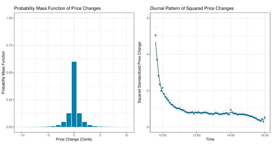
Figure 2: The empirical probability mass function of price changes (left) and average squared price changes in 5 minute and 30 second intraday intervals with a smoothed curve (right) for the IBM stock.

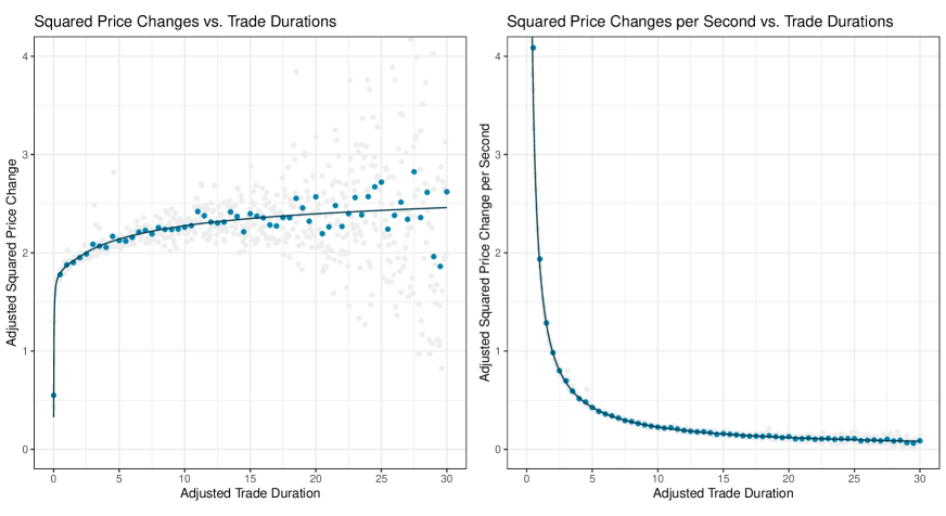
Figure 3: The average diurnally adjusted squared price changes (left) and diurnally adjusted squared price changes per second (right) in 50 millisecond and half second intervals of diurnally adjusted trade durations with a smoothed curve for the IBM stock.

3.4 Dynamics of Intraday Price Volatility

For each trading day, we estimate 10 specifications of the proposed dynamic model – with different parametrizations and different parameters set to zero. The features of the models are summarized in Table 2. In Table 3, we report the minimum, maximum, and median values of estimated parameters. Note that, we do not report p-values as all parameters are significant due to huge numbers of observations (with the exception of $\pi$ for a single day, as further mentioned below). In Table 4, we assess fit of the models using the average log-likelihood and residual autocorrelation tests in the form of R² statistic. Note that the number of parameters (in any of our model specifications) is negligible compared to the number of observations. For this reason, we do not report AIC or BIC.

First, let us focus on the parametrization of the model. We compare the mean-variance parametrization (models I–V), used e.g. by Koopman et al. (2017, 2018) and Alomani et al. (2018), with the proposed mean-overdispersion parametrization (models VI–X). When the mean is not dynamic and is set to zero, both parametrizations are equivalent. The only difference lies in the temporal adjustment, which is based on the squared differences for the mean-variance parametrization and the squared differences with substracted mean in absolute value for the mean-overdispersion parametrization. The results show that this difference is not that distinct – model I has very similar log-likelihood to model VI and model IV to model IX. When the mean is dynamic, however, the mean-overdispersion is superior – models VII, VIII, and X clearly outperform their counterpart models II, III, and V in terms of log-likelihood. The problem, of course, lies in bounds on parameter space imposed by the mean-variance parametrization.

Next, we asses the impact of the individual parameters. As discussed in Section 3.3, the autocorrelation and partial autocorrelation functions of price changes suggest MA(1) structure for the mean process. Indeed, restricting $\theta$ to zero causes considerable decrease in log-likelihood as evident between models IV/V and IX/X. The autocorrelation in residuals also significantly increases. As expected, the estimated $\theta$ is negative for all trading days. Interestingly, its value is much closer to zero in the case of the mean-variance parametrization than the mean-overdispersion parametrization. This suppression of $\theta$ is caused by the lower bound on the variance process. In the mean-overdispersion parametrization, there is no such restriction and the mean process is able to reach its full potential.

The comparison of log-likelihood and autocorrelation in squared residuals between models III/V and VIII/X reveals that volatility (whether paramterized in terms of variance or overdispersion) should not be treated as constant. Similarly to $\theta$, there is a difference in estimated values of $\alpha$ and $\varphi$ between the mean-variance and mean-overdispersion parametrizations. Model X has higher persistence in comparison to model V. Again, this can be atributed to the lower bound on the variance process in the mean-variance parametrization.

In each model allowing for zero inflation, $\pi$ is positive for all days except one, July 28. This suggests that there is an increased occurence of zero price changes in general and the underlying distribution should accomodate this. Among the three components studied in this section – dynamic mean, dynamic volatility, and zero inflation – setting parameter $\pi$ to zero decreases the log-likelihood the least, but still distinctly.

Overall, model X performs the best in terms of the log-likelihood among our 10 candidates. The proposed specification for the mean and overdispersion processes also overwhelmingly reduces residual autocorrelation in price changes and squared price changes. Due to huge number of observations, however, it is difficult to obtain statistical significance of no autocorrelation. The associated Ljung–Box test rejects no autocorrelation in residuals of model X for all days and lags at 0.01 significance level. The associated ARCH-LM test suggests no autocorrelation in squared residuals of model X for 68 percent of days for lag 1 but only 4 percent for lag 100 at 0.01 significance level. Nevertheless, the R² static is very low in all cases and the model captures mean and volatility dynamics quite well.

Table 2: Summary of the features of the estimated models.

Model	Mean	Volatility	Zeros	Parametrization
I	Static	Static	Unaltered	Variance
II	Dynamic	Dynamic	Unaltered	Variance
III	Dynamic	Static	Inflated	Variance
IV	Static	Dynamic	Inflated	Variance
V	Dynamic	Dynamic	Inflated	Variance
VI	Static	Static	Unaltered	Overdispersion
VII	Dynamic	Dynamic	Unaltered	Overdispersion
VIII	Dynamic	Static	Inflated	Overdispersion
IX	Static	Dynamic	Inflated	Overdispersion
X	Dynamic	Dynamic	Inflated	Overdispersion

Table 3: The minimum, median, and maximum values of estimated parameters of various daily models for the IBM stock.

		Variance Models					Overdispersion Models
Coef.	Trans.	I	II	III	IV	V	VI	VII	VIII	IX	X
	Min		-0.149	-0.064		-0.181		-0.449	-0.567		-0.527
$\theta$	Med		-0.103	-0.028		-0.116		-0.302	-0.383		-0.343
	Max		-0.050	-0.006		-0.055		-0.216	-0.305		-0.261
	Min	-0.379	-0.384	-0.379	-0.400	-0.386	-0.212	-0.513	-0.663	-0.196	-0.513
$\omega$	Med	0.200	0.192	0.401	0.299	0.340	0.384	0.068	0.095	0.491	0.170
	Max	0.676	0.712	1.056	0.860	0.958	0.892	0.613	0.885	1.066	0.800
	Min		0.471		0.644	0.468		0.942		0.708	0.954
$\varphi$	Med		0.761		0.834	0.787		0.982		0.872	0.981
	Max		0.963		0.984	0.963		0.997		0.988	0.997
	Min		0.103		0.095	0.102		0.065		0.100	0.077
$\alpha$	Med		0.495		0.498	0.517		0.165		0.488	0.192
	Max		0.667		0.681	0.701		0.259		0.697	0.287
	Min			0.000	0.000	0.000			0.000	0.000	0.000
$\pi$	Med			0.154	0.119	0.118			0.132	0.111	0.119
	Max			0.299	0.235	0.246			0.250	0.223	0.221

Table 4: The R² statistics of residuals and squared residuals regressed on their lagged values with the average log-likelihood of an observation for various daily models for the IBM stock.

		Variance Models					Overdispersion Models
Statistic	Lag	I	II	III	IV	V	VI	VII	VIII	IX	X
	1	0.118	0.040	0.104	0.077	0.041	0.116	0.004	0.002	0.075	0.003
AR R2	10	0.151	0.055	0.136	0.097	0.055	0.149	0.008	0.004	0.095	0.007
	100	0.154	0.057	0.139	0.098	0.057	0.153	0.010	0.007	0.096	0.009
	1	0.104	0.003	0.097	0.005	0.003	0.104	0.000	0.001	0.006	0.000
ARCH R2	10	0.150	0.008	0.145	0.007	0.007	0.154	0.004	0.028	0.007	0.003
	100	0.181	0.021	0.176	0.016	0.018	0.189	0.007	0.049	0.015	0.006
Log-Likelihood		-1.264	-1.200	-1.245	-1.212	-1.193	-1.267	-1.177	-1.187	-1.209	-1.170

3.5 Daily Measures of Price Volatility

The proposed approach can naturally be used to model intraday dynamics of prices but also to estimate volatility at daily level as a model-based alternative to various nonparametric volatility measures. A standard nonparametric measure of daily volatility is the realized variance – the sum of squared returns. However, this measure is biased by market microstructure noise and generally not recommended to use at ultra-high-frequency (see, e.g., Hansen and Lunde, 2006). At lower frequency such as 5 minutes, however, it can be sufficient as the impact of market microstructure noise is reduced (see, e.g., Liu et al., 2015). A widely used realized measure that is robust to market microstructure noise is the realized kernel of Barndorff-Nielsen et al. (2008).

In this section, we compare the realized variance and the realized kernel based on the modified Tukey–Hanning kernel with realized measures implied by our model. The total variance based on the proposed model is given by

$$TMV=\sum_{i=1}^{n}(1-\pi)\left(\lvert\mu_{i}\rvert+\delta_{i}+\pi\mu_{i}^{2}\right).$$ (7)

We can also measure volatility by the total overdispersion adjusted for temporal effects (both diurnal and duration) given by

$$AMV=\sum_{i=1}^{n}\frac{\delta_{i}}{\hat{f}_{\mathrm{disp}}(t_{i})\hat{f}_{\mathrm{rel}}(\tilde{d}_{i})}=\sum_{i=1}^{n}\exp\left(\omega+\varepsilon_{i}\right).$$ (8)

In the latter realized measure, market microstructure noise is filtered by removing the MA(1) component and the effect of trade durations.

Figure 4 shows daily volatility obtained by these measures. The largest variance for all measures is on April 20 (following the announcement of the first quarter results on April 19) and on July 19 (following the announcement of the second quarter results on July 18). We can see that all measures tend to move together but have different scale. This is also supported by a simple correlation analysis. The highest correlations are 0.998 between the total model volatility and the realized variance and 0.965 between the adjusted model volatility and the realized kernel. Other correlations lie between 0.821 and 0.882. We can conclude that the total model volatility is similar to the realized variance as they are both influenced by market microstructure noise. On the other hand, the adjusted model volatility is robust to market microstructure noise, just as the realized kernel. The main benefit of the proposed model-based approach is that we can decompose the variance into individual components according to (2) and (4).

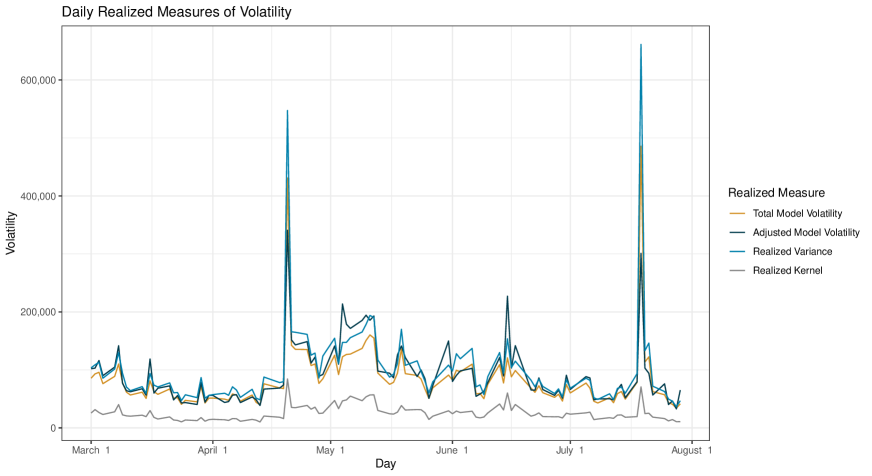
Figure 4: The daily values of various volatility realized measures for the IBM stock.

4 Conclusion

We have proposed a dynamic model for intraday stock prices that takes into account irregularly spaced observations, simultaneous transactions, discreteness of prices, and market microstructure noise. In this model, we have combined two streams of the literature dealing with UHF-GARCH and Skellam-GARCH models respectively and further developed them. We have shown that the model finds its use not only in analysis of intraday dynamics but also in estimation of daily volatility.

Suggestions for future research follow Table 1. Our model can be extended to include dynamics of trade durations and possibly trade volumes. Another direction lies in multivariate modeling. This is, however, quite challenging due to nonsynchronicity of ultra-high-frequency data.

Funding

The work on this paper was supported by the Czech Science Foundation under project 23-06139S and the personal and professional development support program of the Faculty of Informatics and Statistics, Prague University of Economics and Business.

Appendix A Evidence from Further Stocks

In this appendix, we report the results for additional stocks: Caterpillar (CA), traded on NYSE with an average of 2.320 transactions per second; Cisco (CSCO), traded on NASDAQ with an average of 5.738 transactions per second; Electronic Arts (EA), traded on NASDAQ with an average of 1.518 transactions per second; Intel (INTC), traded on NASDAQ with an average of 8.683 transactions per second; Mastercard (MA), traded on NYSE with an average of 2.732 transactions per second; and McDonald’s (MCD), traded on NYSE with an average of 2.402 transactions per second.

In general, these results closely resemble those observed for the IBM stock. Nonetheless, there are two distinctions. First, while smoothing splines effectively capture the diurnal patterns of price volatility in the IBM stock, they struggle to account for the impact of news events occurring at regular times. This discrepancy is particularly pronounced when analyzing the INTC stock. Nonetheless, this isn’t a significant limitation for our study. Second, zero-inflation is not necessary in most days for the CSCO and INTC stocks, which are the two most frequently traded stocks in our sample. Although zero price changes occur more frequently for these stocks compared to others, a regular Skellam distribution suffices. In other aspects, the results reinforce the implications drawn from the analysis of the IBM stock.

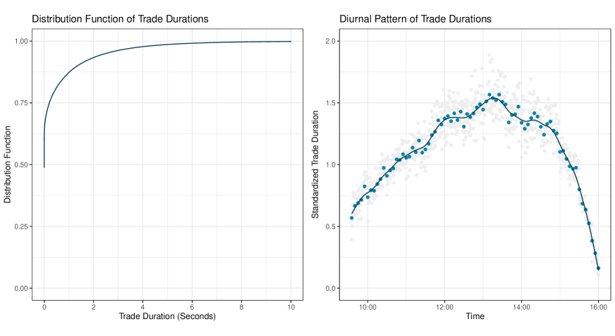
Figure 5: The empirical distribution function of trade durations (left) and average trade durations in 5 minute and 30 second intraday intervals with a smoothed curve (right) for the CAT stock.

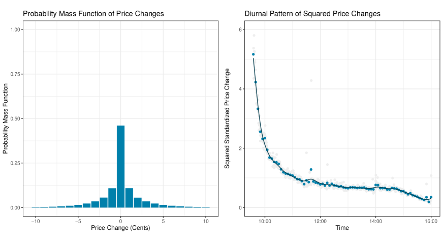
Figure 6: The empirical probability mass function of price changes (left) and average squared price changes in 5 minute and 30 second intraday intervals with a smoothed curve (right) for the CAT stock.

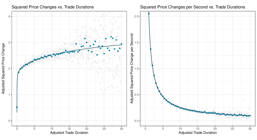
Figure 7: The average diurnally adjusted squared price changes (left) and diurnally adjusted squared price changes per second (right) in 50 millisecond and half second intervals of diurnally adjusted trade durations with a smoothed curve for the CAT stock.

Table 5: The minimum, median, and maximum values of estimated parameters of various daily models for the CAT stock.

		Variance Models					Overdispersion Models
Coef.	Trans.	I	II	III	IV	V	VI	VII	VIII	IX	X
	Min		-0.195	-0.187		-0.268		-0.372	-0.554		-0.509
$\theta$	Med		-0.120	-0.059		-0.155		-0.283	-0.432		-0.387
	Max		-0.074	-0.013		-0.096		-0.217	-0.347		-0.289
	Min	1.122	1.064	1.546	1.318	1.357	1.238	0.904	1.190	1.423	1.178
$\omega$	Med	1.724	1.633	2.147	1.915	1.982	1.834	1.497	1.829	2.023	1.774
	Max	2.817	2.703	3.302	3.070	3.136	2.906	2.655	3.077	3.194	3.005
	Min		0.724		0.821	0.735		0.910		0.859	0.937
$\varphi$	Med		0.908		0.950	0.933		0.957		0.950	0.971
	Max		0.986		0.996	0.990		0.993		0.995	0.997
	Min		0.026		0.021	0.029		0.025		0.020	0.025
$\alpha$	Med		0.200		0.199	0.221		0.210		0.190	0.204
	Max		0.434		0.421	0.463		0.287		0.416	0.297
	Min			0.217	0.177	0.176			0.202	0.166	0.179
$\pi$	Med			0.277	0.237	0.237			0.256	0.226	0.232
	Max			0.343	0.317	0.318			0.325	0.313	0.309

Table 6: The R² statistics of residuals and squared residuals regressed on their lagged values with the average log-likelihood of an observation for various daily models for the CAT stock.

		Variance Models					Overdispersion Models
Statistic	Lag	I	II	III	IV	V	VI	VII	VIII	IX	X
	1	0.117	0.040	0.092	0.092	0.043	0.115	0.005	0.003	0.091	0.004
AR R2	10	0.153	0.056	0.123	0.117	0.058	0.150	0.011	0.005	0.115	0.006
	100	0.156	0.058	0.126	0.119	0.060	0.154	0.013	0.008	0.117	0.009
	1	0.099	0.007	0.085	0.016	0.008	0.099	0.001	0.003	0.017	0.001
ARCH R2	10	0.137	0.009	0.127	0.017	0.010	0.139	0.003	0.038	0.018	0.003
	100	0.173	0.017	0.162	0.022	0.016	0.177	0.008	0.065	0.023	0.006
Log-Likelihood		-2.057	-1.947	-1.948	-1.908	-1.881	-2.050	-1.923	-1.889	-1.907	-1.857

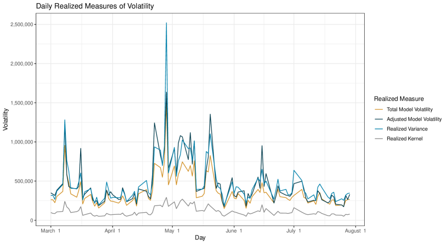
Figure 8: The daily values of various volatility realized measures for the CAT stock.

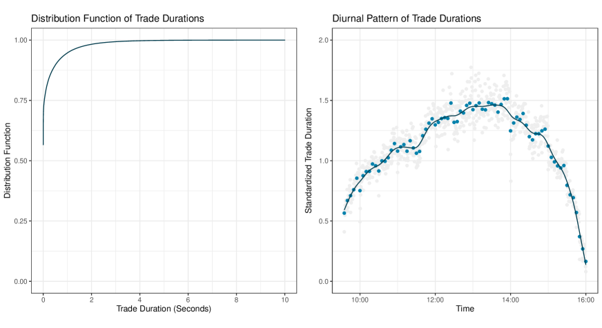
Figure 9: The empirical distribution function of trade durations (left) and average trade durations in 5 minute and 30 second intraday intervals with a smoothed curve (right) for the CSCO stock.

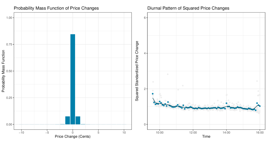
Figure 10: The empirical probability mass function of price changes (left) and average squared price changes in 5 minute and 30 second intraday intervals with a smoothed curve (right) for the CSCO stock.

Figure 11: The average diurnally adjusted squared price changes (left) and diurnally adjusted squared price changes per second (right) in 50 millisecond and half second intervals of diurnally adjusted trade durations with a smoothed curve for the CSCO stock.

Table 7: The minimum, median, and maximum values of estimated parameters of various daily models for the CSCO stock.

		Variance Models					Overdispersion Models
Coef.	Trans.	I	II	III	IV	V	VI	VII	VIII	IX	X
	Min		-0.091	-0.013		-0.090		-0.571	-0.620		-0.571
$\theta$	Med		-0.056	-0.007		-0.056		-0.466	-0.483		-0.469
	Max		-0.015	-0.002		-0.018		-0.252	-0.266		-0.252
	Min	-1.784	-1.876	-1.784	-1.924	-1.876	-1.729	-2.640	-2.695	-1.796	-2.640
$\omega$	Med	-1.659	-1.714	-1.659	-1.736	-1.716	-1.601	-2.251	-2.316	-1.622	-2.250
	Max	-1.466	-1.467	-1.014	-1.451	-1.345	-1.386	-1.750	-1.856	-1.289	-1.750
	Min		0.533		0.670	0.533		0.978		0.731	0.978
$\varphi$	Med		0.752		0.843	0.752		0.998		0.887	0.998
	Max		0.984		0.986	0.983		1.000		0.986	1.000
	Min		0.100		0.113	0.100		0.014		0.111	0.014
$\alpha$	Med		0.789		0.746	0.788		0.079		0.720	0.079
	Max		1.323		1.071	1.323		0.240		1.120	0.299
	Min			0.000	0.000	0.000			0.000	0.000	0.000
$\pi$	Med			0.000	0.000	0.000			0.000	0.000	0.000
	Max			0.317	0.179	0.176			0.154	0.199	0.152

Table 8: The R² statistics of residuals and squared residuals regressed on their lagged values with the average log-likelihood of an observation for various daily models for the CSCO stock.

		Variance Models					Overdispersion Models
Statistic	Lag	I	II	III	IV	V	VI	VII	VIII	IX	X
	1	0.126	0.058	0.122	0.075	0.058	0.123	0.000	0.000	0.072	0.000
AR R2	10	0.174	0.084	0.170	0.101	0.083	0.165	0.004	0.003	0.095	0.004
	100	0.178	0.085	0.173	0.102	0.084	0.168	0.005	0.004	0.096	0.005
	1	0.094	0.005	0.093	0.006	0.005	0.091	0.000	0.000	0.008	0.000
ARCH R2	10	0.130	0.011	0.129	0.008	0.010	0.125	0.002	0.004	0.010	0.002
	100	0.158	0.020	0.157	0.015	0.019	0.148	0.006	0.018	0.014	0.006
Log-Likelihood		-0.512	-0.480	-0.510	-0.488	-0.480	-0.516	-0.448	-0.451	-0.489	-0.448

Figure 12: The daily values of various volatility realized measures for the CSCO stock.

Figure 13: The empirical distribution function of trade durations (left) and average trade durations in 5 minute and 30 second intraday intervals with a smoothed curve (right) for the EA stock.

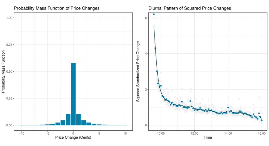
Figure 14: The empirical probability mass function of price changes (left) and average squared price changes in 5 minute and 30 second intraday intervals with a smoothed curve (right) for the EA stock.

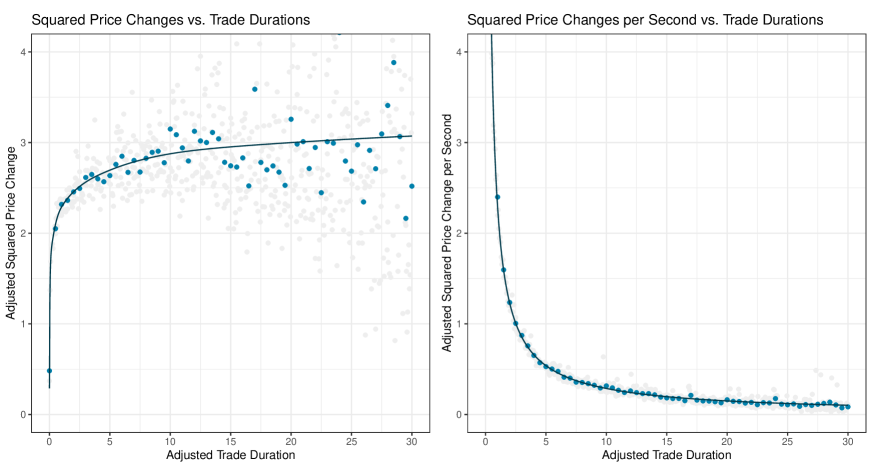
Figure 15: The average diurnally adjusted squared price changes (left) and diurnally adjusted squared price changes per second (right) in 50 millisecond and half second intervals of diurnally adjusted trade durations with a smoothed curve for the EA stock.

Table 9: The minimum, median, and maximum values of estimated parameters of various daily models for the EA stock.

		Variance Models					Overdispersion Models
Coef.	Trans.	I	II	III	IV	V	VI	VII	VIII	IX	X
	Min		-0.124	-0.095		-0.202		-0.365	-0.631		-0.536
$\theta$	Med		-0.073	-0.035		-0.103		-0.242	-0.416		-0.352
	Max		-0.020	-0.003		-0.032		-0.133	-0.242		-0.179
	Min	0.262	0.115	0.633	0.468	0.476	0.361	-0.183	0.232	0.506	0.176
$\omega$	Med	0.878	0.761	1.324	1.091	1.135	0.979	0.650	1.008	1.194	0.981
	Max	2.135	1.917	3.201	3.074	2.738	2.270	1.628	2.497	3.063	2.086
	Min		0.683		0.629	0.671		0.847		0.545	0.897
$\varphi$	Med		0.916		0.950	0.945		0.954		0.949	0.971
	Max		0.994		0.999	0.998		0.997		1.000	0.999
	Min		0.043		0.017	0.020		0.031		0.008	0.032
$\alpha$	Med		0.177		0.184	0.190		0.188		0.184	0.189
	Max		0.433		0.491	0.496		0.346		0.484	0.347
	Min			0.161	0.137	0.138			0.150	0.127	0.140
$\pi$	Med			0.317	0.263	0.266			0.292	0.249	0.261
	Max			0.468	0.445	0.416			0.435	0.390	0.387

Table 10: The R² statistics of residuals and squared residuals regressed on their lagged values with the average log-likelihood of an observation for various daily models for the EA stock.

		Variance Models					Overdispersion Models
Statistic	Lag	I	II	III	IV	V	VI	VII	VIII	IX	X
	1	0.101	0.043	0.087	0.074	0.045	0.099	0.006	0.002	0.072	0.004
AR R2	10	0.134	0.058	0.118	0.093	0.060	0.131	0.013	0.005	0.091	0.007
	100	0.141	0.061	0.125	0.096	0.063	0.139	0.017	0.010	0.094	0.011
	1	0.094	0.008	0.086	0.013	0.009	0.092	0.001	0.002	0.014	0.001
ARCH R2	10	0.136	0.010	0.130	0.015	0.012	0.135	0.003	0.028	0.016	0.003
	100	0.170	0.020	0.164	0.022	0.019	0.170	0.011	0.052	0.023	0.009
Log-Likelihood		-1.590	-1.491	-1.514	-1.462	-1.446	-1.582	-1.467	-1.455	-1.460	-1.422

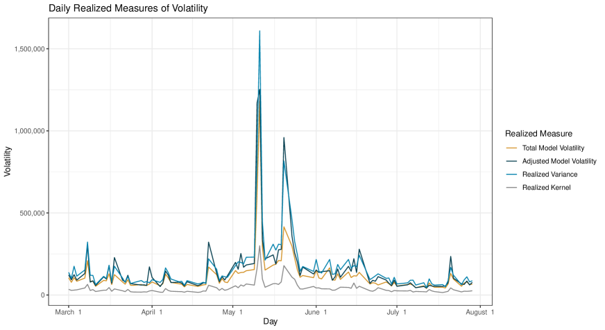
Figure 16: The daily values of various volatility realized measures for the EA stock.

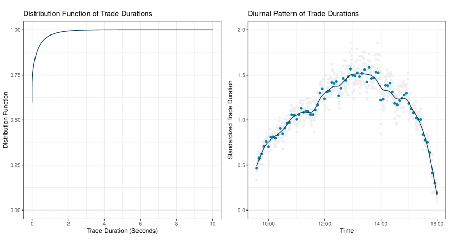
Figure 17: The empirical distribution function of trade durations (left) and average trade durations in 5 minute and 30 second intraday intervals with a smoothed curve (right) for the INTC stock.

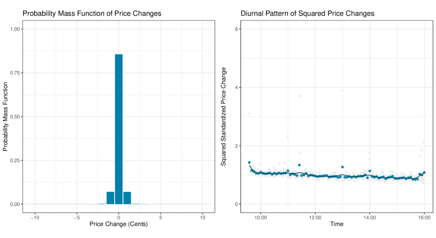
Figure 18: The empirical probability mass function of price changes (left) and average squared price changes in 5 minute and 30 second intraday intervals with a smoothed curve (right) for the INTC stock.

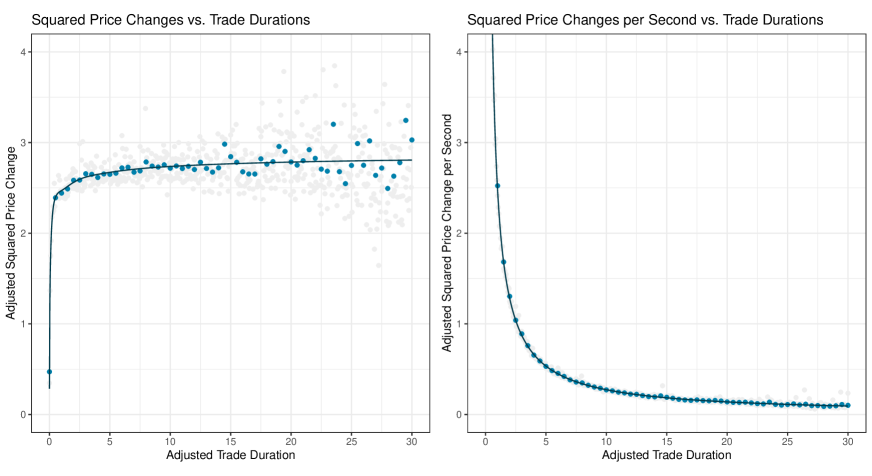
Figure 19: The average diurnally adjusted squared price changes (left) and diurnally adjusted squared price changes per second (right) in 50 millisecond and half second intervals of diurnally adjusted trade durations with a smoothed curve for the INTC stock.

Table 11: The minimum, median, and maximum values of estimated parameters of various daily models for the INTC stock.

		Variance Models					Overdispersion Models
Coef.	Trans.	I	II	III	IV	V	VI	VII	VIII	IX	X
	Min		-0.080	-0.012		-0.081		-0.693	-0.697		-0.693
$\theta$	Med		-0.050	-0.006		-0.050		-0.519	-0.526		-0.519
	Max		-0.012	-0.001		-0.011		-0.329	-0.337		-0.329
	Min	-1.930	-2.131	-1.930	-2.105	-2.061	-1.904	-3.160	-3.047	-2.051	-3.160
$\omega$	Med	-1.760	-1.849	-1.760	-1.875	-1.839	-1.723	-2.516	-2.548	-1.812	-2.516
	Max	-1.570	-1.611	-1.570	-1.638	-1.616	-1.531	-1.194	-2.145	-1.509	-1.212
	Min		0.540		0.740	0.540		0.989		0.798	0.988
$\varphi$	Med		0.772		0.872	0.772		0.999		0.893	0.999
	Max		0.974		0.982	0.977		1.000		0.992	1.000
	Min		0.102		0.104	0.107		0.010		0.107	0.010
$\alpha$	Med		0.895		0.842	0.894		0.047		0.839	0.047
	Max		1.325		1.018	1.324		0.208		1.027	0.208
	Min			0.000	0.000	0.000			0.000	0.000	0.000
$\pi$	Med			0.000	0.000	0.000			0.000	0.000	0.000
	Max			0.000	0.063	0.102			0.028	0.074	0.016

Table 12: The R² statistics of residuals and squared residuals regressed on their lagged values with the average log-likelihood of an observation for various daily models for the INTC stock.

		Variance Models					Overdispersion Models
Statistic	Lag	I	II	III	IV	V	VI	VII	VIII	IX	X
	1	0.132	0.061	0.129	0.079	0.061	0.131	0.000	0.000	0.077	0.000
AR R2	10	0.186	0.091	0.182	0.109	0.090	0.183	0.003	0.003	0.106	0.003
	100	0.188	0.092	0.185	0.109	0.091	0.185	0.004	0.004	0.106	0.004
	1	0.096	0.005	0.095	0.008	0.005	0.095	0.000	0.000	0.009	0.000
ARCH R2	10	0.143	0.012	0.142	0.010	0.012	0.139	0.002	0.003	0.011	0.002
	100	0.175	0.029	0.174	0.022	0.029	0.165	0.006	0.016	0.020	0.007
Log-Likelihood		-0.464	-0.436	-0.461	-0.442	-0.435	-0.467	-0.399	-0.401	-0.443	-0.399

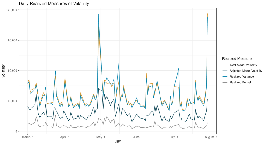
Figure 20: The daily values of various volatility realized measures for the INTC stock.

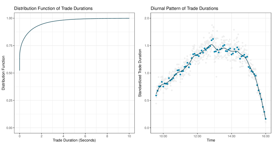
Figure 21: The empirical distribution function of trade durations (left) and average trade durations in 5 minute and 30 second intraday intervals with a smoothed curve (right) for the MA stock.

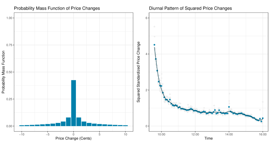
Figure 22: The empirical probability mass function of price changes (left) and average squared price changes in 5 minute and 30 second intraday intervals with a smoothed curve (right) for the MA stock.

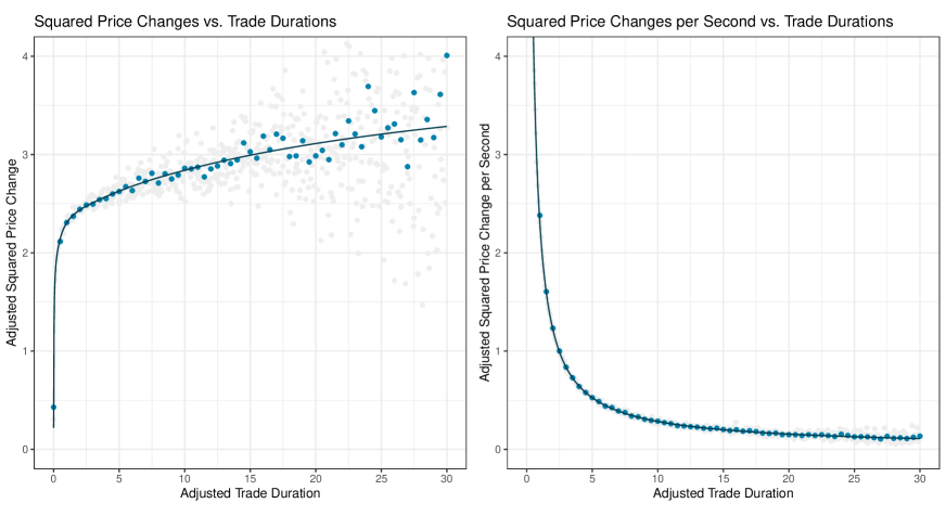
Figure 23: The average diurnally adjusted squared price changes (left) and diurnally adjusted squared price changes per second (right) in 50 millisecond and half second intervals of diurnally adjusted trade durations with a smoothed curve for the MA stock.

Table 13: The minimum, median, and maximum values of estimated parameters of various daily models for the MA stock.

		Variance Models					Overdispersion Models
Coef.	Trans.	I	II	III	IV	V	VI	VII	VIII	IX	X
	Min		-0.197	-0.238		-0.351		-0.432	-0.552		-0.528
$\theta$	Med		-0.118	-0.106		-0.167		-0.312	-0.468		-0.445
	Max		-0.078	-0.041		-0.098		-0.216	-0.392		-0.325
	Min	2.495	2.264	2.923	1.602	2.689	2.539	2.032	2.671	0.745	2.261
$\omega$	Med	3.218	2.949	3.722	3.444	3.456	3.263	2.741	3.421	3.500	3.204
	Max	3.974	4.061	4.000	3.994	4.004	3.903	3.800	3.892	3.913	3.916
	Min		0.420		0.442	0.287		0.800		0.385	0.866
$\varphi$	Med		0.953		0.986	0.963		0.976		0.982	0.989
	Max		1.000		1.000	1.000		1.000		1.000	1.000
	Min		0.001		0.000	0.000		0.000		0.000	0.000
$\alpha$	Med		0.047		0.021	0.031		0.050		0.020	0.033
	Max		0.169		0.149	0.155		0.167		0.147	0.154
	Min			0.250	0.000	0.231			0.244	0.234	0.228
$\pi$	Med			0.332	0.322	0.323			0.329	0.317	0.319
	Max			0.388	0.394	0.398			0.386	0.395	0.387

Table 14: The R² statistics of residuals and squared residuals regressed on their lagged values with the average log-likelihood of an observation for various daily models for the MA stock.

		Variance Models					Overdispersion Models
Statistic	Lag	I	II	III	IV	V	VI	VII	VIII	IX	X
	1	0.125	0.055	0.086	0.118	0.061	0.123	0.005	0.007	0.118	0.008
AR R2	10	0.167	0.081	0.121	0.157	0.087	0.165	0.015	0.010	0.156	0.012
	100	0.170	0.083	0.123	0.159	0.089	0.167	0.017	0.013	0.157	0.014
	1	0.090	0.030	0.061	0.056	0.030	0.088	0.009	0.004	0.058	0.004
ARCH R2	10	0.122	0.038	0.099	0.068	0.045	0.121	0.020	0.035	0.071	0.020
	100	0.149	0.044	0.126	0.077	0.054	0.149	0.025	0.058	0.081	0.026
Log-Likelihood		-2.736	-2.626	-2.466	-2.451	-2.415	-2.734	-2.586	-2.413	-2.455	-2.382

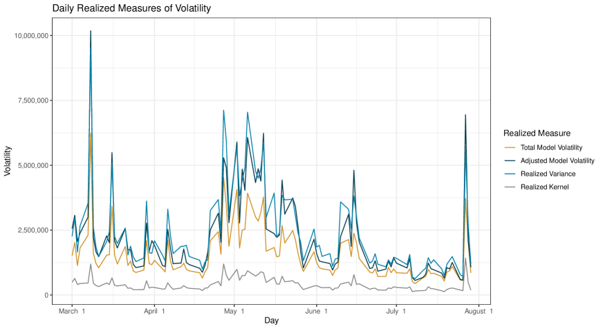
Figure 24: The daily values of various volatility realized measures for the MA stock.

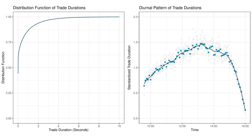
Figure 25: The empirical distribution function of trade durations (left) and average trade durations in 5 minute and 30 second intraday intervals with a smoothed curve (right) for the MCD stock.

Figure 26: The empirical probability mass function of price changes (left) and average squared price changes in 5 minute and 30 second intraday intervals with a smoothed curve (right) for the MCD stock.

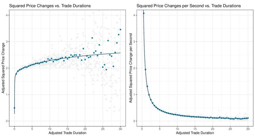
Figure 27: The average diurnally adjusted squared price changes (left) and diurnally adjusted squared price changes per second (right) in 50 millisecond and half second intervals of diurnally adjusted trade durations with a smoothed curve for the MCD stock.

Table 15: The minimum, median, and maximum values of estimated parameters of various daily models for the MCD stock.

		Variance Models					Overdispersion Models
Coef.	Trans.	I	II	III	IV	V	VI	VII	VIII	IX	X
	Min		-0.173	-0.135		-0.231		-0.377	-0.568		-0.490
$\theta$	Med		-0.112	-0.045		-0.138		-0.297	-0.443		-0.394
	Max		-0.054	-0.008		-0.064		-0.232	-0.358		-0.305
	Min	1.017	0.980	1.275	1.127	1.159	1.125	0.776	0.961	1.226	0.987
$\omega$	Med	1.466	1.383	1.802	1.578	1.616	1.573	1.212	1.473	1.684	1.446
	Max	2.556	2.381	2.938	2.744	2.832	2.648	2.353	2.688	2.911	2.630
	Min		0.745		0.821	0.783		0.904		0.817	0.942
$\varphi$	Med		0.899		0.946	0.924		0.958		0.945	0.974
	Max		0.992		0.996	0.996		0.999		0.999	0.998
	Min		0.030		0.029	0.018		0.021		0.027	0.019
$\alpha$	Med		0.223		0.217	0.235		0.211		0.214	0.211
	Max		0.425		0.461	0.466		0.278		0.435	0.308
	Min			0.185	0.144	0.139			0.169	0.133	0.148
$\pi$	Med			0.251	0.205	0.203			0.225	0.191	0.204
	Max			0.343	0.310	0.307			0.325	0.303	0.299

Table 16: The R² statistics of residuals and squared residuals regressed on their lagged values with the average log-likelihood of an observation for various daily models for the MCD stock.

		Variance Models					Overdispersion Models
Statistic	Lag	I	II	III	IV	V	VI	VII	VIII	IX	X
	1	0.123	0.047	0.102	0.095	0.050	0.120	0.005	0.003	0.094	0.004
AR R2	10	0.162	0.065	0.138	0.122	0.067	0.158	0.011	0.005	0.119	0.006
	100	0.166	0.067	0.141	0.124	0.069	0.162	0.013	0.008	0.121	0.008
	1	0.098	0.007	0.086	0.014	0.008	0.097	0.001	0.002	0.014	0.000
ARCH R2	10	0.147	0.008	0.139	0.015	0.010	0.148	0.003	0.040	0.016	0.002
	100	0.190	0.020	0.181	0.021	0.018	0.192	0.007	0.073	0.022	0.006
Log-Likelihood		-1.941	-1.833	-1.861	-1.814	-1.788	-1.933	-1.806	-1.792	-1.812	-1.760

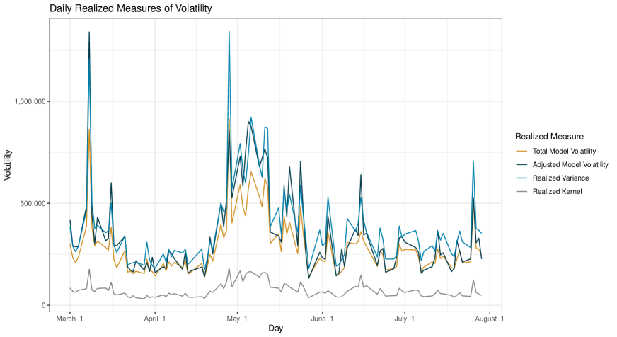
Figure 28: The daily values of various volatility realized measures for the MCD stock.

References

- Aït-Sahalia et al. (2005) Aït-Sahalia Y, Mykland PA, Zhang L (2005). “How Often to Sample a Continuous-Time Process in the Presence of Market Microstructure Noise.” The Review of Financial Studies, 18(2), 351–416. ISSN 0893-9454. https://doi.org/10.1093/rfs/hhi016.
- Alomani et al. (2018) Alomani GA, Alzaid AA, Omair MA (2018). “A Skellam GARCH model.” Brazilian Journal of Probability and Statistics, 32(1), 200–214. ISSN 0103-0752. https://doi.org/10.1214/16-bjps338.
- Alzaid and Omair (2010) Alzaid AA, Omair MA (2010). “On the Poisson Difference Distribution Inference and Applications.” Bulletin of the Malaysian Mathematical Sciences Society, 33(1), 17–45. ISSN 0126-6705. http://eudml.org/doc/244475.
- Barndorff-Nielsen et al. (2008) Barndorff-Nielsen OE, Hansen PR, Lunde A, Shephard N (2008). “Designing Realized Kernels to Measure the ex post Variation of Equity Prices in the Presence of Noise.” Econometrica, 76(6), 1481–1536. ISSN 0012-9682. https://doi.org/10.3982/ecta6495.
- Barndorff-Nielsen et al. (2009) Barndorff-Nielsen OE, Hansen PR, Lunde A, Shephard N (2009). “Realized Kernels in Practice: Trades and Quotes.” Econometrics Journal, 12(3), 1–32. ISSN 1368-4221. https://doi.org/10.1111/j.1368-423X.2008.00275.x.
- Barndorff-Nielsen et al. (2011) Barndorff-Nielsen OE, Hansen PR, Lunde A, Shephard N (2011). “Multivariate Realised Kernels: Consistent Positive Semi-Definite Estimators of the Covariation of Equity Prices with Noise and Non-Synchronous Trading.” Journal of Econometrics, 162(2), 149–169. ISSN 0304-4076. https://doi.org/10.1016/j.jeconom.2010.07.009.
- Barndorff-Nielsen et al. (2012) Barndorff-Nielsen OE, Pollard DG, Shephard N (2012). “Integer-Valued Lévy Processes and Low Latency Financial Econometrics.” Quantitative Finance, 12(4), 587–605. ISSN 1469-7688. https://doi.org/10.1080/14697688.2012.664935.
- Blasques et al. (2018) Blasques F, Gorgi P, Koopman SJ, Wintenberger O (2018). “Feasible Invertibility Conditions and Maximum Likelihood Estimation for Observation-Driven Models.” Electronic Journal of Statistics, 12(1), 1019–1052. ISSN 1935-7524. https://doi.org/10.1214/18-ejs1416.
- Blasques et al. (2022a) Blasques F, Holý V, Tomanová P (2022a). “Zero-Inflated Autoregressive Conditional Duration Model for Discrete Trade Durations with Excessive Zeros.” https://arxiv.org/abs/1812.07318.
- Blasques et al. (2015) Blasques F, Koopman SJ, Lucas A (2015). “Information-Theoretic Optimality of Observation-Driven Time Series Models for Continuous Responses.” Biometrika, 102(2), 325–343. ISSN 0006-3444. https://doi.org/10.1093/biomet/asu076.
- Blasques et al. (2021) Blasques F, Lucas A, van Vlodrop AC (2021). “Finite Sample Optimality of Score-Driven Volatility Models: Some Monte Carlo Evidence.” Econometrics and Statistics, 19, 47–57. ISSN 2452-3062. https://doi.org/10.1016/j.ecosta.2020.03.010.
- Blasques et al. (2022b) Blasques F, van Brummelen J, Koopman SJ, Lucas A (2022b). “Maximum Likelihood Estimation for Score-Driven Models.” Journal of Econometrics, 227(2), 325–346. ISSN 0304-4076. https://doi.org/10.1016/j.jeconom.2021.06.003.
- Bollerslev (1986) Bollerslev T (1986). “Generalized Autoregressive Conditional Heteroskedasticity.” Journal of Econometrics, 31(3), 307–327. ISSN 0304-4076. https://doi.org/10.1016/0304-4076(86)90063-1.
- Bollerslev (1987) Bollerslev T (1987). “A Conditionally Heteroskedastic Time Series Model for Speculative Prices and Rates of Return.” Review of Economics and Statistics, 69(3), 542–547. ISSN 0034-6535. https://doi.org/10.2307/1925546.
- Buccheri et al. (2021) Buccheri G, Bormetti G, Corsi F, Lillo F (2021). “A Score-Driven Conditional Correlation Model for Noisy and Asynchronous Data: An Application to High-Frequency Covariance Dynamics.” Journal of Business & Economic Statistics, 39(4), 920–936. ISSN 0735-0015. https://doi.org/10.1080/07350015.2020.1739530.
- Catania et al. (2022) Catania L, Di Mari R, Santucci de Magistris P (2022). “Dynamic Discrete Mixtures for High-Frequency Prices.” Journal of Business & Economic Statistics, 40(2), 559–577. ISSN 0735-0015. https://doi.org/10.1080/07350015.2020.1840994.
- Creal et al. (2013) Creal D, Koopman SJ, Lucas A (2013). “Generalized Autoregressive Score Models with Applications.” Journal of Applied Econometrics, 28(5), 777–795. ISSN 0883-7252. https://doi.org/10.1002/jae.1279.
- Cui et al. (2021) Cui Y, Li Q, Zhu F (2021). “Modeling Z-Valued Time Series Based on New Versions of the Skellam INGARCH Model.” Brazilian Journal of Probability and Statistics, 35(2), 293–314. ISSN 0103-0752. https://doi.org/10.1214/20-bjps473.
- Doukhan et al. (2021) Doukhan P, Khan NM, Neumann MH (2021). “Mixing Properties of Integer-Valued GARCH Processes.” Alea - Latin American Journal of Probability and Mathematical Statistics, 18(1), 401–420. ISSN 1980-0436. https://doi.org/10.30757/alea.v18-18.
- Engle (2002) Engle R (2002). “New Frontiers for ARCH Models.” Journal of Applied Econometrics, 17(5), 425–446. ISSN 0883-7252. https://doi.org/10.1002/jae.683.
- Engle (1982) Engle RF (1982). “Autoregressive Conditional Heteroscedasticity with Estimates of the Variance of United Kingdom Inflation.” Econometrica, 50(4), 987–1007. ISSN 0012-9682. https://doi.org/10.2307/1912773.
- Engle (2000) Engle RF (2000). “The Econometrics of Ultra-High-Frequency Data.” Econometrica, 68(1), 1–22. ISSN 0012-9682. https://doi.org/10.1111/1468-0262.00091.
- Engle and Russell (1998) Engle RF, Russell JR (1998). “Autoregressive Conditional Duration: A New Model for Irregularly Spaced Transaction Data.” Econometrica, 66(5), 1127–1162. ISSN 0012-9682. https://doi.org/10.2307/2999632.