Abstract

The description of distributions related to grain microstructure helps physicists to understand the processes in materials and their properties. This paper presents a general statistical methodology for the analysis of crystallographic orientations of grains in a 3D Laguerre tessellation dataset which represents the microstructure of a polycrystalline material. We introduce complex stochastic models which may substitute expensive laboratory experiments: conditional on the Laguerre tessellation, we suggest interaction models for the distribution of cubic crystal lattice orientations, where the interaction is between pairs of orientations for neighbouring grains in the tessellation. We discuss parameter estimation and model comparison methods based on maximum pseudolikelihood as well as graphical procedures for model checking using simulations. Our methodology is applied for analysing a dataset representing a nickel-titanium shape memory alloy.

Keywords: Cubic crystal orientation, fundamental zone, model comparison, pairwise interaction models, pseudolikelihood, simulation

1   Introduction

In a previous paper by some of us [28] we developed models for the Laguerre tessellation describing the morphology of polycrystalline datasets. The present paper concerns statistical methodology for analysing crystallographic orientations (henceforth ’orientations’) of grains conditional on that the set of grains forms a Laguerre tessellation. Including orientations as additional marks is crucial for applications in physics and material engineering, cf. [10], and leads us to consider complex interaction models for the distribution of orientations [19] conditioned on a Laguerre tessellation, as opposed to previous studies based on models for the distribution of individual orientations, see e.g. [1, 4, 9, 15, 17].

1.1   Motivation and related results

The microstructure of polycrystalline materials is characterized by the morphology of grains and the spatial redistribution of orientations among the grains. The distribution of orientations is often nonuniform and some preferential orientations occur. This phenomenon is in material science called a texture [10], and it determines the elastic properties of the material, which describe how much each grain deforms under external forces. The topic of fitting the orientation distribution has a long history, see e.g. [3, 26]. On the one hand, nonparametric kernel estimation methods have been developed [5], which may be suitable for electron backscatter diffraction (3D-EBSD) measurements [30]. On the other hand, parametric models and estimation of the orientation probability density have been suggested [1], and also maximum likelihood estimation for the Bingham distribution using the EM algorithm has been proposed [22].

The deformation of grains is affected not only by the orientation of each grain but also by the orientations of its neighbouring grains [13]. Since the grains are space-filling with pairwise disjoint interiors, they constitute a tessellation, and a very flexible class of tessellation models are so-called Laguerre tessellations [16]. Statistical models and estimation procedures for Laguerre tessellations describing the grain structure in polycrystalline materials have been developed in [28]. Moreover, using the two statistical tests introduced in [23], it was shown that the tessellation and orientations should not be generally treated separately. Nevertheless, in the earlier work mentioned above, the problem of the estimation of the orientation distribution is considered independently of the tessellation, hence not taking into account the geometry of the grain structure.

Based on experimentally measured 3D microstructure obtained by X-ray diffraction (3D-XRD) [25] or by 3D-EBSD [29, 30], physicists and material engineers study the effect of the orientation distribution on the elastic properties of the material [8, 14]. However, as these are expensive methods of microscopy, we are motivated to propose a complementary, less expensive statistical approach as developed in the following.

1.2   Our contribution and outline

Our goal is to offer statistical models and simulation procedures for the joint distribution of the orientations when we condition on the underlying tessellation. In particular, we account for the dependencies between orientations of neighbouring grains. To the best of our knowledge, such models have not been introduced before in the literature. Due to the complexity of the data it may be too ambitious to aim at a model fitting all aspects seen in the data. Moreover, orientation characteristics as considered in this paper are of interest in material science research [8, 14, 18]. Therefore, when fitting models we will concentrate on these orientation characteristics as illustrated at the end of this paper.

Perhaps our most important contribution is the modelling part. We start with a rather flexible semiparametric model not accounting for the dependence on the tessellation and with independence between grain orientations. Then we use the Laguerre tessellation constructed in [24], and extend the model to more complex models incorporating dependencies between the tessellation and orientations: conditional on the tessellation, we model dependencies between orientations for neighbouring grains; then we extend this by adding various weights as detailed in Section 4.

The paper is organized as follows. Section 2 provides the needed background for various orientation representations, where invariance under the group of symmetries of a cube is a natural assumption, as well as orientation characteristics used for model specification and comparison. Section 3 introduces a dataset of a microstructure of metallic material used in later sections to illustrate our statistical approach. Section 4 presents our three parametric classes, followed in Section 5 by methods for parameter estimation, model comparison and model checking as well as simulation. The methodology in Sections 4 and 5 is illustrated in Section 6.

2   Orientation representations and characteristics

2.1   The fundamental region for the case of a cubic lattice structure

The kind of data we study in this paper are ‘crystallographic orientations’ observed in polycrystalline materials where each grain is comprised of atoms forming a cubic lattice structure [10]. To make the meaning of this more precise we need to introduce an equivalence relation and some notation. Let $C_{1},\dots,C_{n}$ be a finite collection of grains which are closed 3-dimensional sets, their interiors are pairwise disjoint and their union $W=C_{1}\cup\ldots\cup C_{n}$ is a connected set in 3-dimensional Euclidean space, which we equip with a coordinate system with axes $x$, $y$ and $z$. In other words, the grains are the cells of a tessellation (subdivision) of $W$ which we refer to as the ‘specimen’. Let $\mathrm{SO}(3)$ be the special orthogonal group, that is, the set of $3\times 3$ rotation matrices with determinant $1$. Let $\mathcal{O}$ be the subgroup of $\mathrm{SO}(3)$ given by the symmetries of a cube. There are 48 symmetries and $\mathcal{O}$ has 24 elements [20]. We consider two elements $G_{1}$ and $G_{2}$ of $\mathrm{SO}(3)$ to be equivalent if $G_{1}=HG_{2}$ for some $H\in\mathcal{O}$. The equivalence classes of this relation form a partition of $\mathrm{SO}(3)$ and a transversal is a set of

representatives in the equivalence class sense. Below we define a particular set $F$ which we call the fundamental zone and which ’effectively’ is a transversal (more precisely, apart from a nullset with respect to the measure in (2) below, $F$ is a transversal whose more complicated definition is given in A). By a crystallographic orientation we mean an element of $\mathrm{SO}(3)$ or just of $F$ because of the equivalence relation.

It is convenient to represent every matrix $G\in\mathrm{SO}(3)$ by its Euler angles $\left(\varphi_{1},\,\phi,\,\varphi_{2}\right)\in[0,2\pi)\times[0,\pi]\times[0,2\pi)$ (determining sequential rotations around the $z$-axis, the $x$-axis and again the $z$-axis, see [10, Section 2.6]). Henceforth, we identify $G$ and $\left(\varphi_{1},\,\phi,\,\varphi_{2}\right)$ without any mentioning, and we use the symbol $g$ as a general notation for both.

Now, define the fundamental zone by

$$F=\big{\{}(\varphi_{1},\,\phi,\,\varphi_{2})\mid\varphi_{1}\in[0,\,2\pi),\ \varphi_{2}\in[0,\,\pi/2),\ \phi\in[\phi_{0}(\varphi_{2}),\,\pi/2]\big{\}},$$ (1)

where

$$\phi_{0}(\varphi_{2})=\arccos~{}\text{min}\left(\dfrac{\cos\varphi_{2}}{\sqrt{1+\cos^{2}\varphi_{2}}},\dfrac{\sin\varphi_{2}}{\sqrt{1+\sin^{2}\varphi_{2}}}\right).$$

2.2   Random orientation representations

By a random orientation we understand a random variable with values in the corresponding space, that is, either $\mathrm{SO}(3)$ for an orientation matrix representation or $[0,2\pi)\times[0,\pi]\times[0,2\pi)$ for an Euler angles representation, where these spaces are equipped with the corresponding Borel $\sigma$-algebra. Since we pay attention to crystallographic orientation in the setting of Section 2.1, we restrict attention to distributions on $F$. Then, by adding an independent uniform distribution on $\mathcal{O}$, this easily extends to a distribution on $\mathrm{SO}(3)$.

For notional convenience we do not distinguish between whether $G,\varphi_{1},\phi,\varphi_{2}$ or another variable introduced in the following refers to a realisation of some random variable, the random variable itself or an argument of a function describing some properties of the random variable. Its meaning will always be obvious from the context.

Let $\mu$ be the normalized (that is, $\mu$ is a probability measure) Haar measure [11] on $\mathrm{SO}(3)$. Then the random orientation distributed according to $\mu$ has the uniform distribution and in terms of Euler angles, for any Borel set $B\subseteq[0,2\pi)\times[0,\pi]\times[0,2\pi)$,

$$\mu(B)=\frac{1}{8\pi^{2}}\int_{0}^{2\pi}\int_{0}^{\pi}\int_{0}^{2\pi}\sin(\phi)\bm{1}{\left[(\varphi_{1},\phi,\varphi_{2})\in B\right]}\,{\rm d}\varphi_{1}\,{\rm d}\phi\,{\rm d}\varphi_{2},$$ (2)

where $\bm{1}[\cdot]$ is the indicator function. Thus the corresponding random Euler angles $\varphi_{1},\phi,\varphi_{2}$ are independent, with $\varphi_{1}$ and $\varphi_{2}$ uniformly distributed on $[0,2\pi)$, and $\eta=\cos\phi$ uniformly distributed on $[-1,1]$.

In later sections we consider various probability density functions. When a single orientation is considered, the density is always with respect to $\mu_{F}$, the restriction of $\mu$ to $F$. When a vector of $n$ orientations is considered, the density is always with respect to the product measure of $\mu_{F}$ $n$ times.

In many places of this paper it becomes useful to consider the ‘transformed orientation’ $t(\varphi_{1},\phi,\,\varphi_{2})=(\varphi_{1},\,\eta,\,\varphi_{2})$ living in the ‘transformed fundamental zone’ given by

$$t(F)=\big{\{}(\varphi_{1},\,\eta,\,\varphi_{2})\mid\varphi_{1}\in[0,\,2\pi),\ \varphi_{2}\in[0,\,\pi/2),\ \eta\in\left[0,\cos\phi_{0}(\varphi_{2})\right]\big{\}}.$$ (3)

It follows from (2) that for any Borel set $B\subseteq t(F)$ the measure $\mu_{F}$ transformed by $t$ is given by

$$\begin{split}t\mu_{F}(B)&=\int_{t(F)}\bm{1}{\left[(\varphi_{1},\eta,\varphi_{2})\in B\right]}\,{\rm d}(\varphi_{1},\eta,\varphi_{2})\\ &=\int_{0}^{2\pi}\int_{0}^{\pi/2}\int_{0}^{\cos\phi_{0}(\varphi_{2})}\bm{1}{\left[(\varphi_{1},\eta,\varphi_{2})\in B\right]}\,{\rm d}\eta\,{\rm d}\varphi_{2}\,{\rm d}\varphi_{1}.\end{split}$$ (4)

Figure 2 shows a graphical representation of $t(F)$ by a cross-section for an arbitrarily chosen value of $\varphi_{1}$.

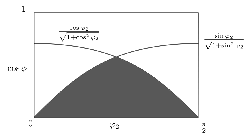
Figure 1: A cross-section of $t(F)$ (black area) given by (3) for an arbitrary $\varphi_{1}\in[0,2\pi)$.

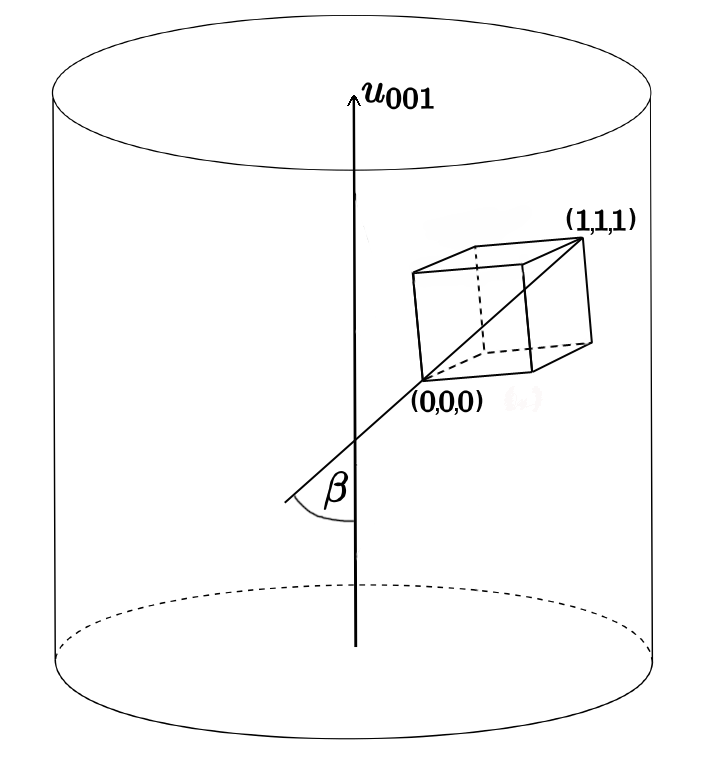
Figure 2: The angle $\beta$ specifies the tilt given by $\cos\beta$ of $v=(1,1,1)^{\top}$ with respect to a particular orientation $G$, cf. (5). Here, the specimen is assumed to be a cylinder with a coordinate system such that the $z$-axis agrees with the axis of the cylinder.

2.3   Orientation characteristics

This section introduces various orientation characteristics where we start by considering a single orientation, then a pair of orientations, and finally a sample of orientations.

To characterize an orientation, some low-dimensional characteristics can be used, e.g. a ‘tilt’

$$\text{tilt}(G;v)=\max_{S\in\,\mathcal{O}}\frac{v^{\top}SGu_{001}}{\|v\|},$$ (5)

where $G$ is an orientation matrix of a grain, $v$ is a chosen direction with respect to a coordinate system specifying the cubic lattice structure of the grain and $u_{001}=(0,0,1)^{\top}$ corresponds to the $z$-axis of the specimen (this is the choice for our application but any unit vector could be used instead). In other words, in order to compute $\text{tilt}(G;v)$, we first compute the cosine of angles between the $z$-axis (in the coordinate system for the specimen) and all equivalent directions of $v$ according to the orientation matrix $G$. Then we choose the largest value. For the data analyzed in this paper, as argued in Section 3, we choose $v$ to be the main diagonal of the cubic lattice, $v=(1,1,1)^{\top}$, see Figure 2.

A natural question is how to measure the closeness of two orientations. The most common measure for two orientations $g_{1}$ and $g_{2}$ is the ‘disorientation angle’ [10, Section 2.7.2] which is given by

$$\operatorname*{dis}(g_{1},g_{2})=\min_{S\in\mathcal{O}}\arccos\frac{{\rm tr}\left(G_{1}^{-1}SG_{2}\right)-1}{2},$$ (6)

where $G_{1}$ and $G_{2}$ are the orientation matrix representations corresponding to $g_{1}$ and $g_{2}$, respectively, and ${\rm tr}$ means the trace of a matrix. Similar orientations have a disorientation angle close to 0 and the maximum disorientation angle is approximately $62.8^{\circ}$. Incidentally, the disorientation angle follows the Mackenzie distribution if $g_{1}$ and $g_{2}$ are considered to be independent random variables following the ‘uniform’ distribution given by the Haar measure in (2) [19, Section 7].

In (6) all 24 elements of $\mathcal{O}$ must be considered. Another measure of closeness of two orientations, which is faster to compute, is the inner product of the embedding $\mathbf{t}$ introduced in [1] and given by

$$\operatorname*{inn}(g_{1},g_{2})=\langle\mathbf{t}(G_{1}),\mathbf{t}(G_{2})\rangle=\sum\limits_{i=1}^{3}\sum\limits_{j=1}^{3}\left(G_{1i}^{\top}G_{2j}\right)^{4}-\frac{9}{5},$$ (7)

where $G_{ki}$ is the $i$th row of the matrix $G_{k}$, $k=1,2$ (since the definition of $\mathbf{t}$ is rather technical, we refer to [1] for details). On the contrary to the disorientation angle, this inner product can be both negative and positive, and closeness corresponds to high values (the maximum value is $6/5$).

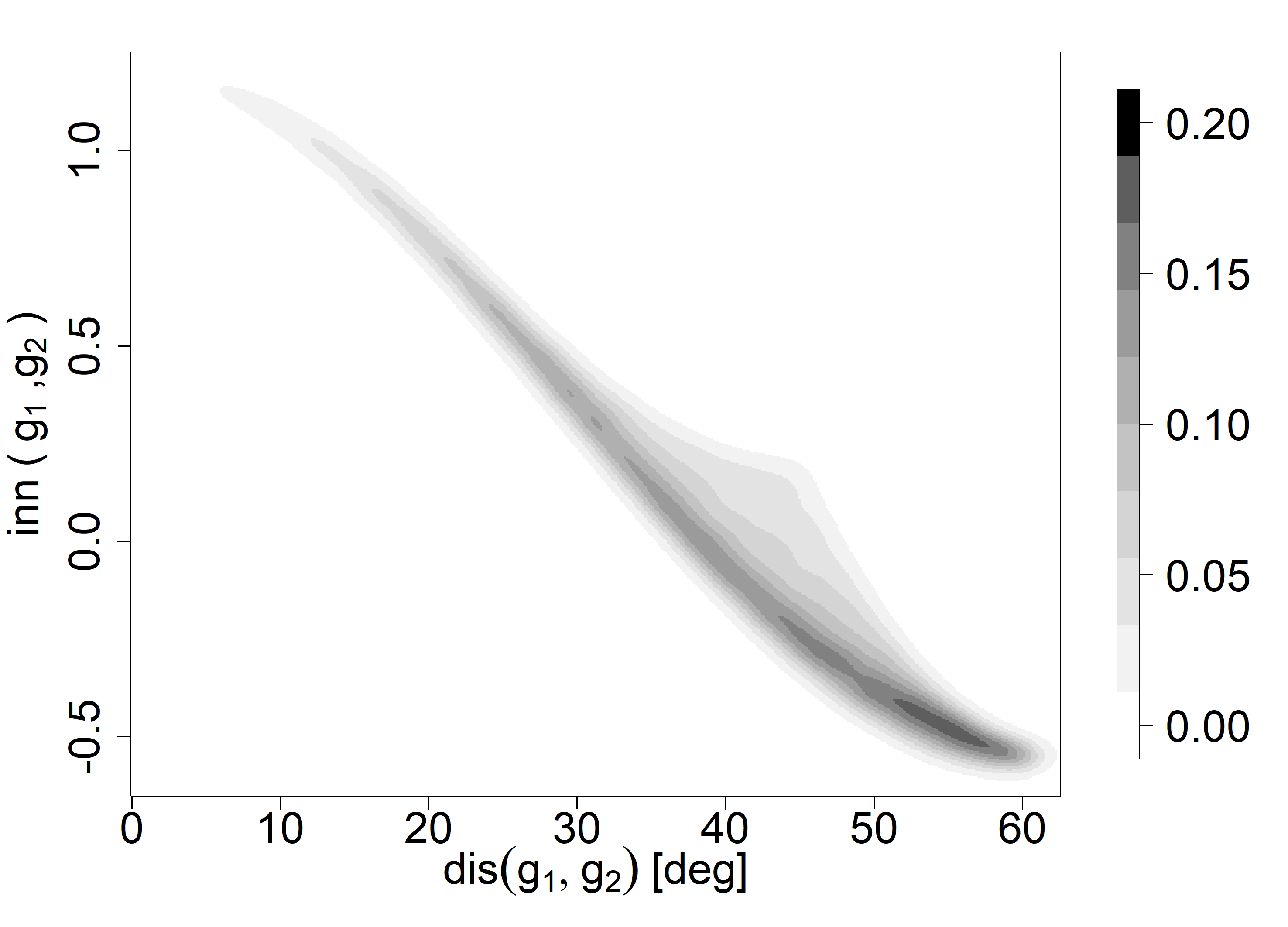
(a) Uniform distribution.

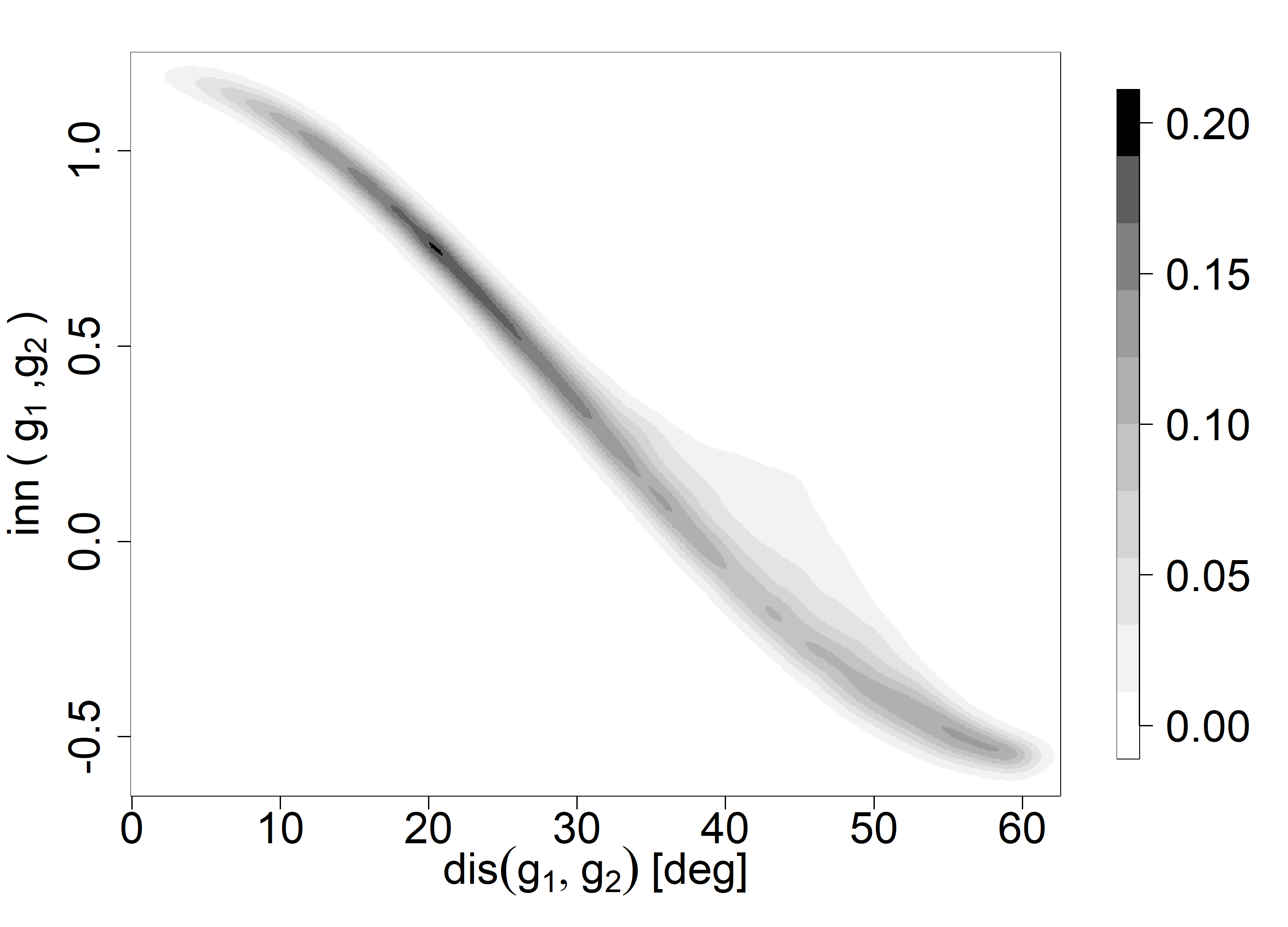
(b) NiTi data.

Figure 3: Kernel density estimators of the bivariate distribution of the inner product $\operatorname*{inn}(g_{1},g_{2})$ and the disorientation angle $\operatorname*{dis}(g_{1},g_{2})$ from (a) the simulated uniform orientation distribution and (b) the NiTi dataset (introduced in Section 3).

To understand the relationship between the measures in (6) and (7), we simulated their joint distribution when $g_{1}$ and $g_{2}$ are considered to be independent random variables following the Haar measure in (2), see Figure 3(a). As expected the disorientation angle and the inner product are strongly negatively correlated, with the Spearman rank correlation coefficient equal to $-0.969$.

Finally, for a sample $g_{1},\dots,g_{n}$ of orientations, [1] introduced a certain scalar $\hat{d}$ which has an interpretation as a sample dispersion (its precise definition is technical, so again we refer to [1]). For later use, note that $0\leq\hat{d}\leq 6/5$, where $\hat{d}=0$ if the $g_{i}$ are equal.

3   Data example

In this section we introduce the data used to illustrate our methodology in the rest of the paper. Briefly, the data comes from [27] and concerns an experiment of a nickel-titanium (NiTi) wire evaluated by the 3D-XRD method. The centroids, volumes and orientations were determined for the microstructure, but no information about the neighbouring structure was provided, so we obtained this information using the construction of the Laguerre tessellation in the article [24]. The data presents a cutout consisting of $n=1060$ grains, the centroids of which lie in a rectangular parallelepiped of size $44\times 44\times 40\,\mu{\rm m}^{3}$, situated in the central part of the wire. Henceforth, we use the notation $\mathbf{C}_{n}=(C_{1},\dots,C_{n})$ for the grains (or cells) of the tessellation and $\mathbf{g}_{n}=(g_{1},\dots,g_{n})$ for the corresponding orientations.

In [13] it was argued using graphical methods that the orientations are not uniformly distributed. In particular, the authors noticed that the orientations are concentrated so that the $z$-axis of the specimen is aligned with a crystal direction given by the main diagonal of a cube (direction $(1,1,1)^{\top}$). This alignment motivates us to use the tilt in (5) with ${v=(1,1,1)^{\top}}$ as a characteristic when we consider a model checking procedure in Section 6.

To visualise the transformed orientations within the transformed fundamental zone, we first divide the domain of $\varphi_{1}$ into $9$ subintervals $[a_{i},a_{i+1})$ of equal length, so ${a_{i}=2\pi i/9}$, $i=0,\dots,9$. For each $i=0,\dots,8$ we obtain a scatter plot of pairs $(\cos\phi,\,\varphi_{2})$ with the corresponding $\varphi_{1}$ in $[a_{i},a_{i+1})$. Figure 4 shows such cross-sections for the data in hand. We observe a higher concentration of points around the larger values of $\cos\phi$. This indicates the presence of a preferential orientation (but it is implausible to determine the specific preferential orientation from the figure).

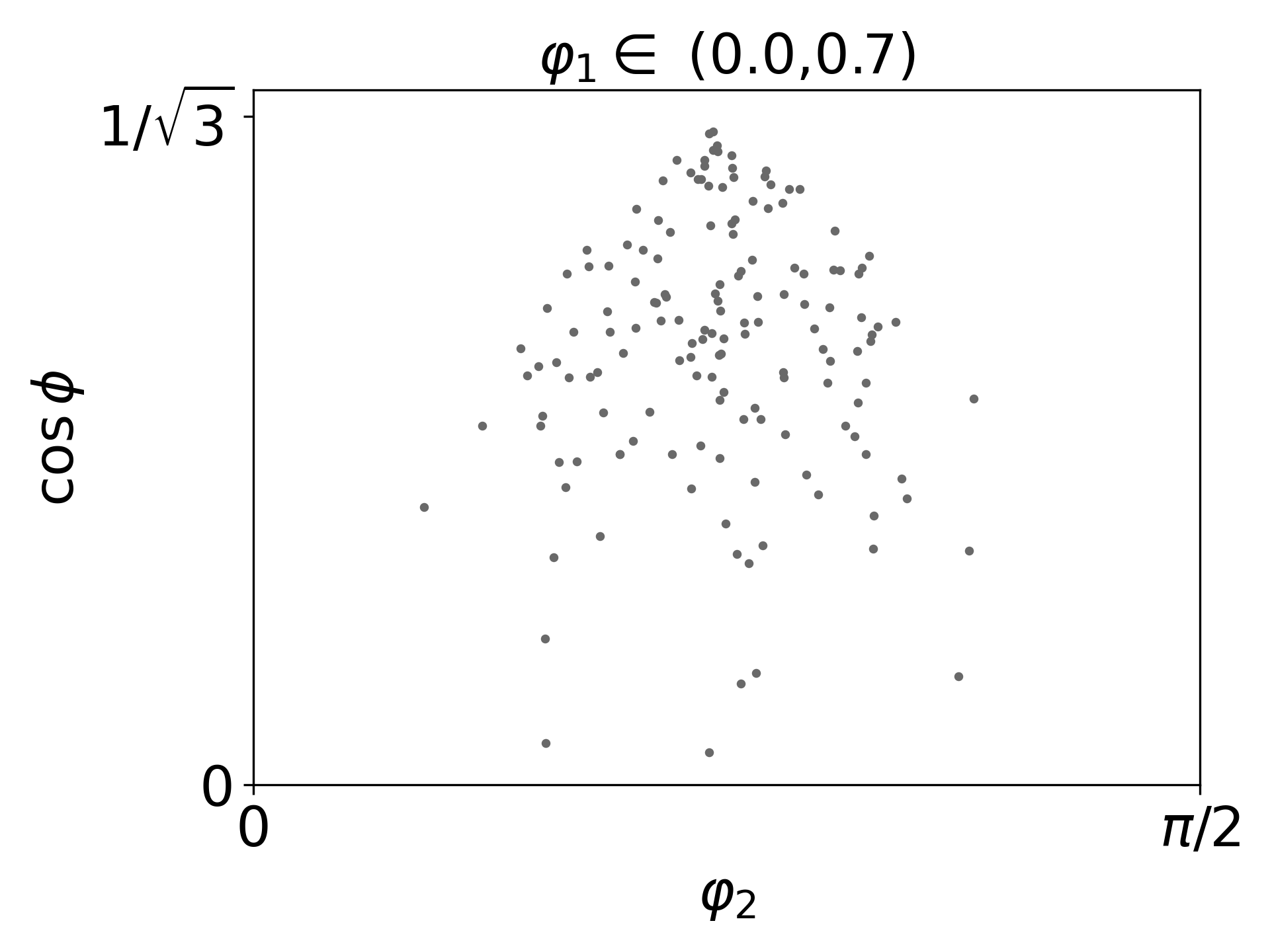
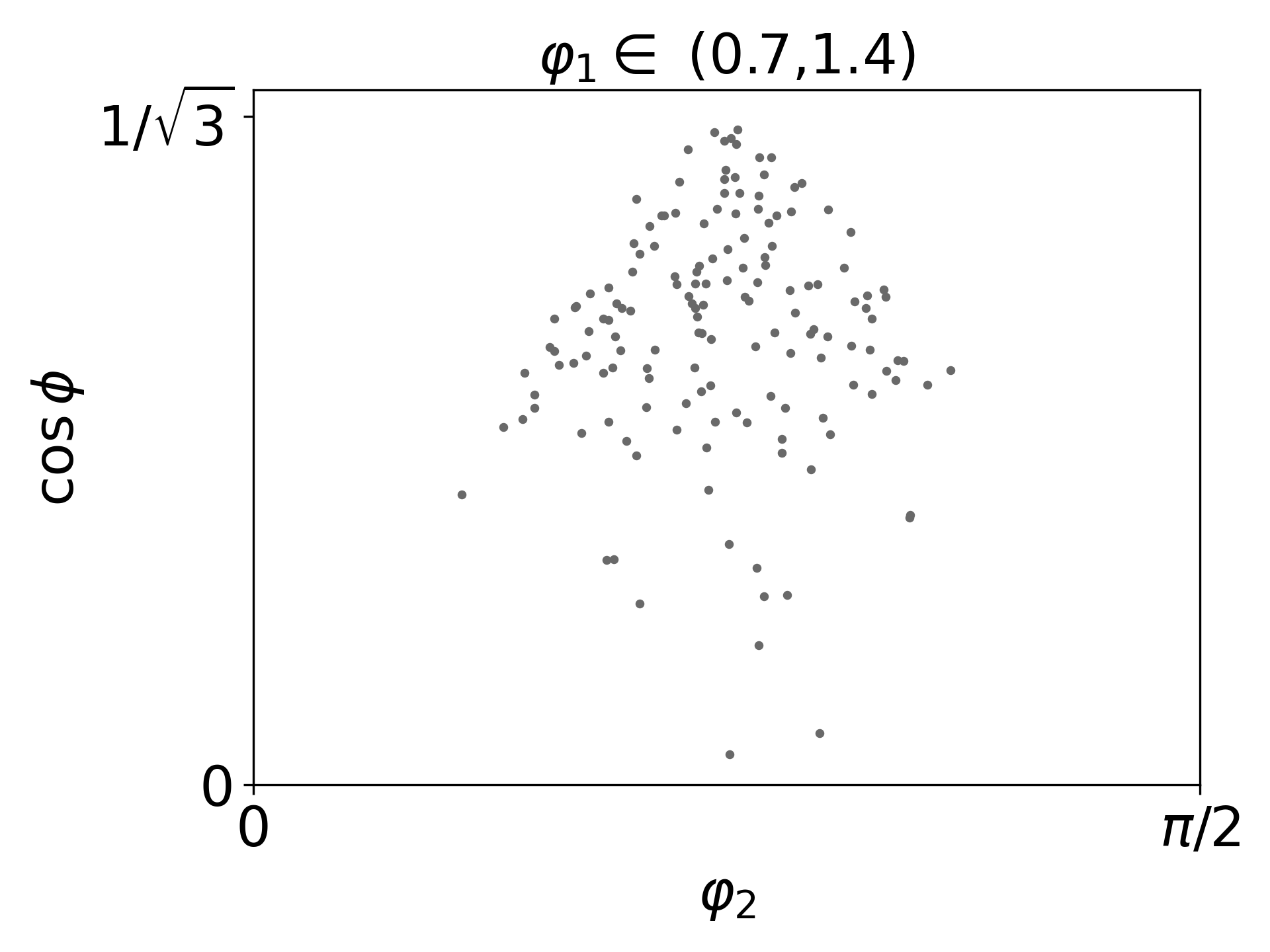
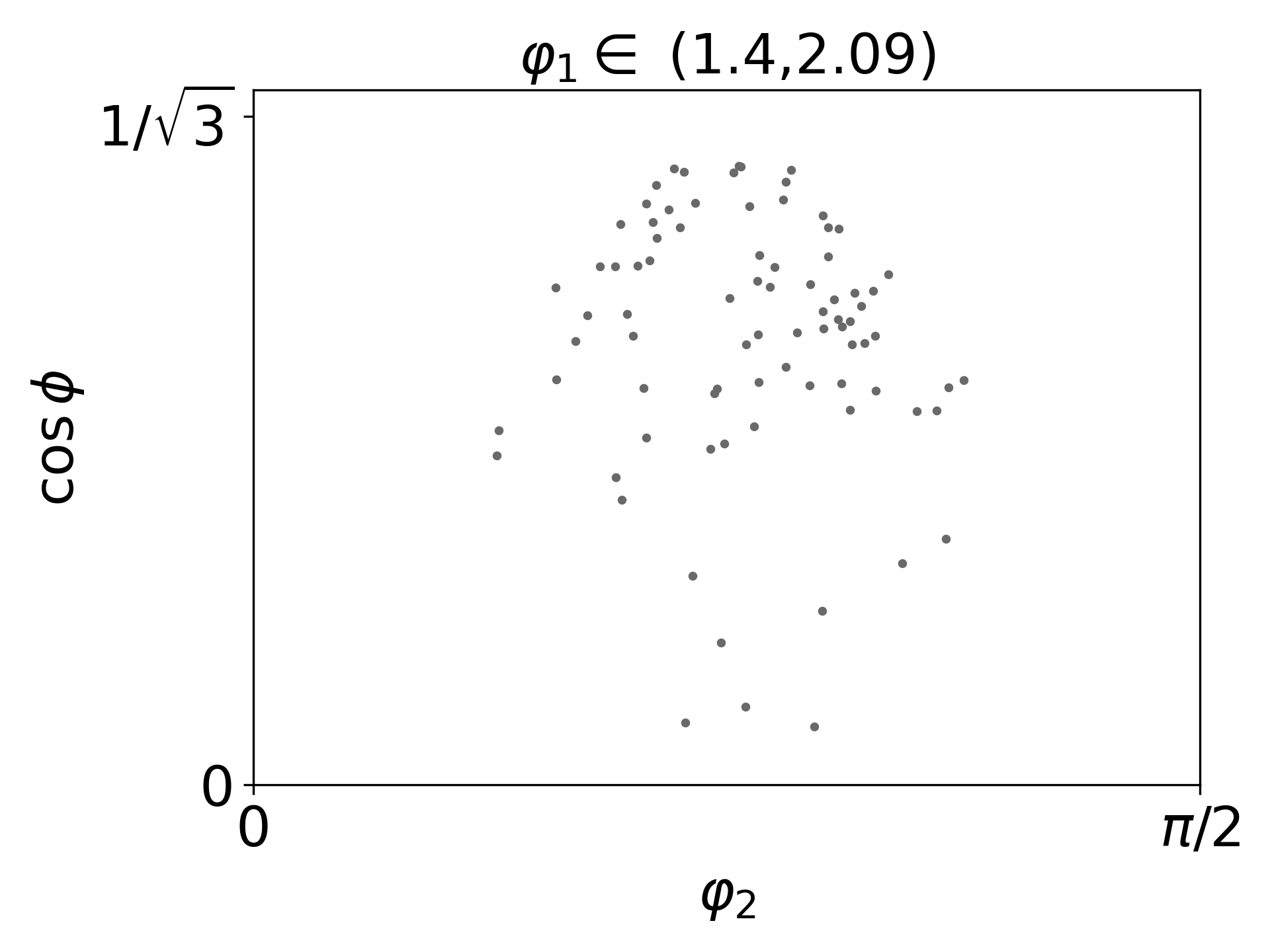
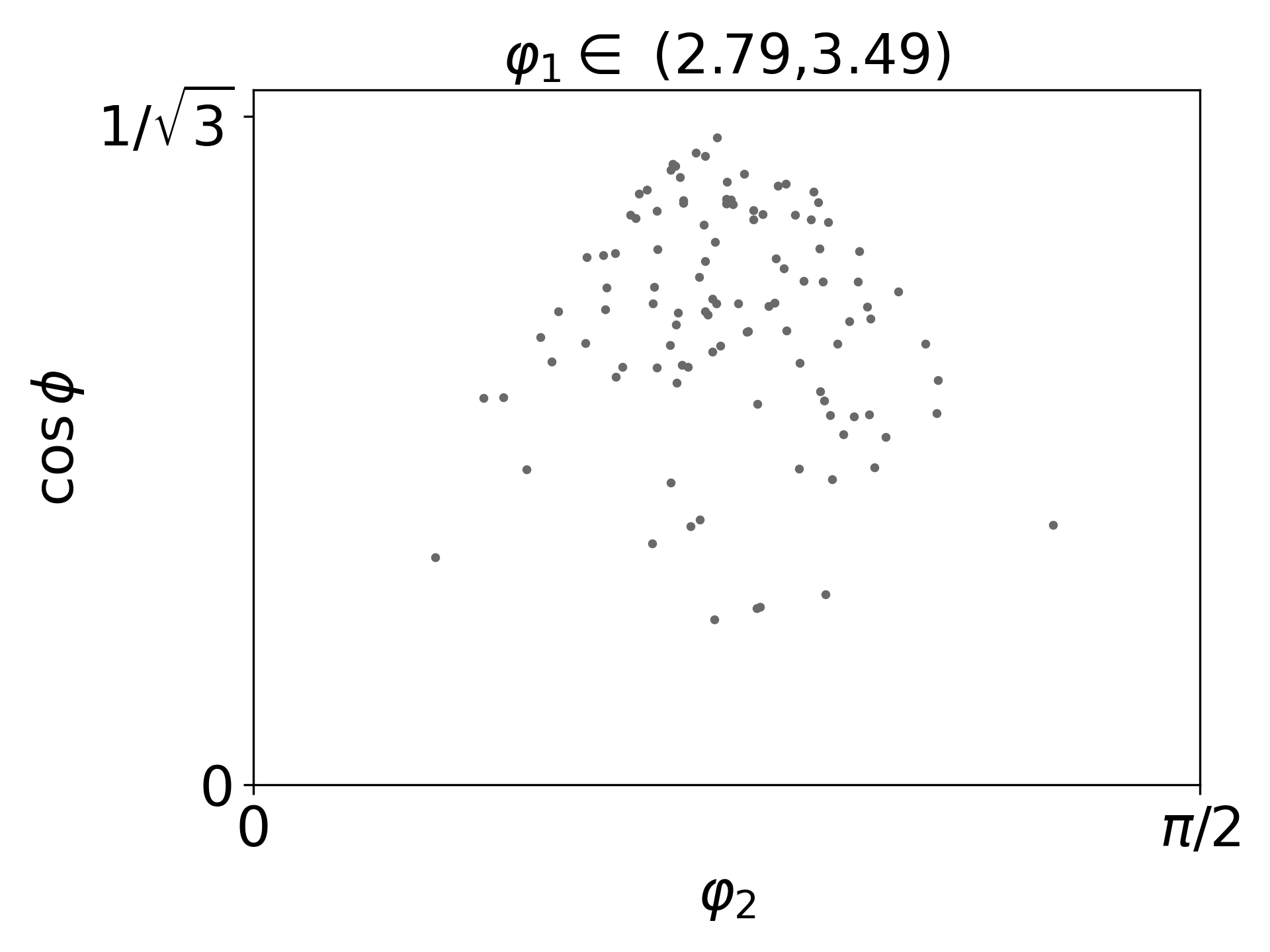
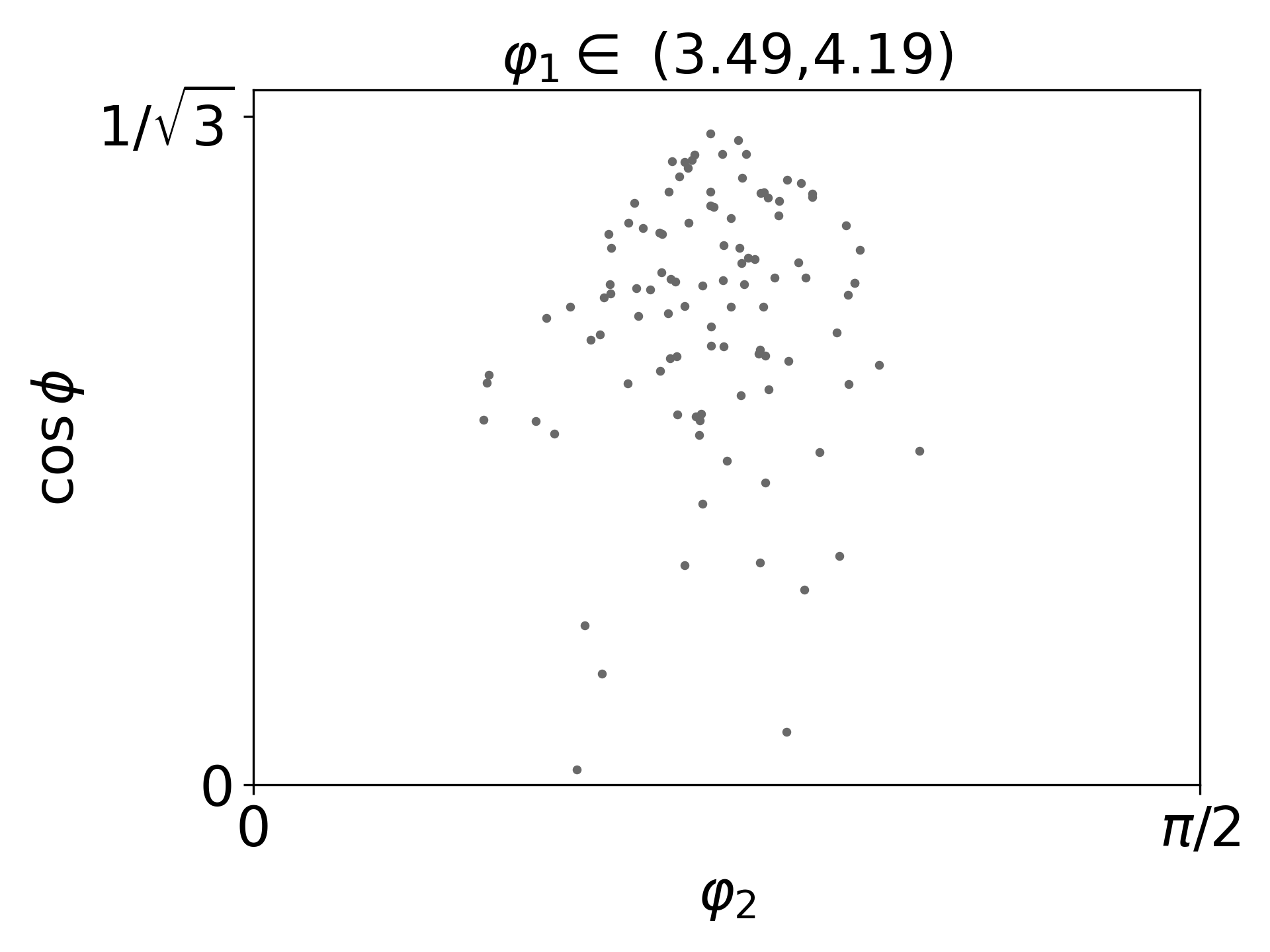
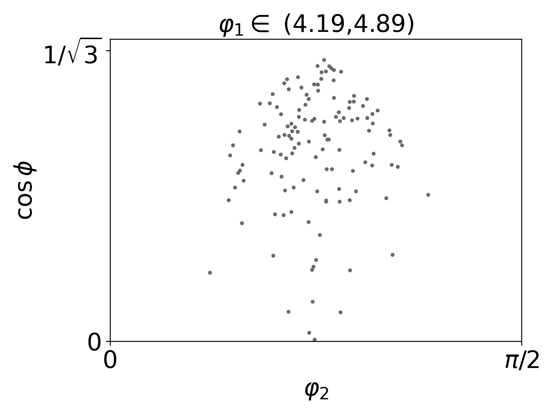
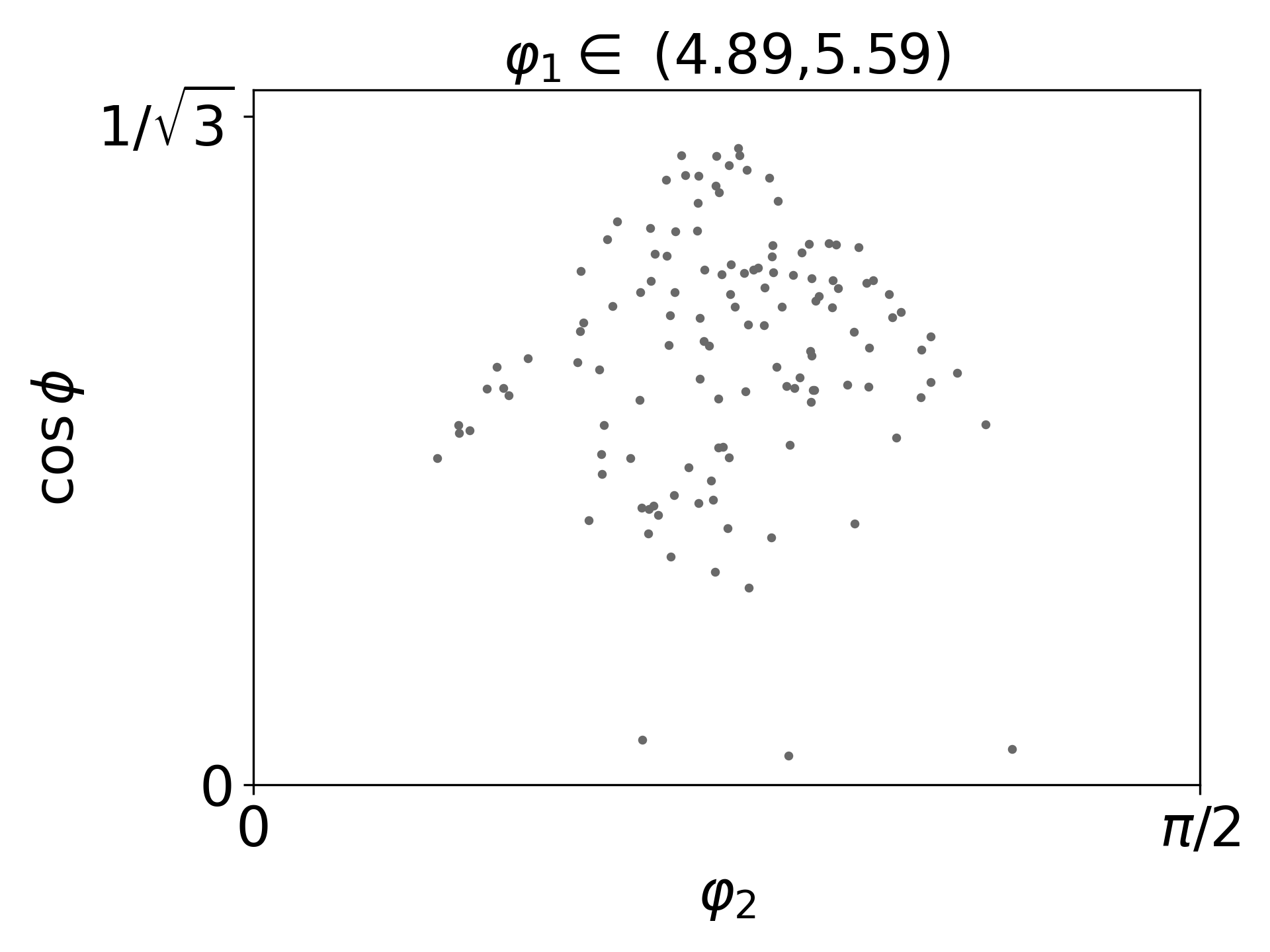
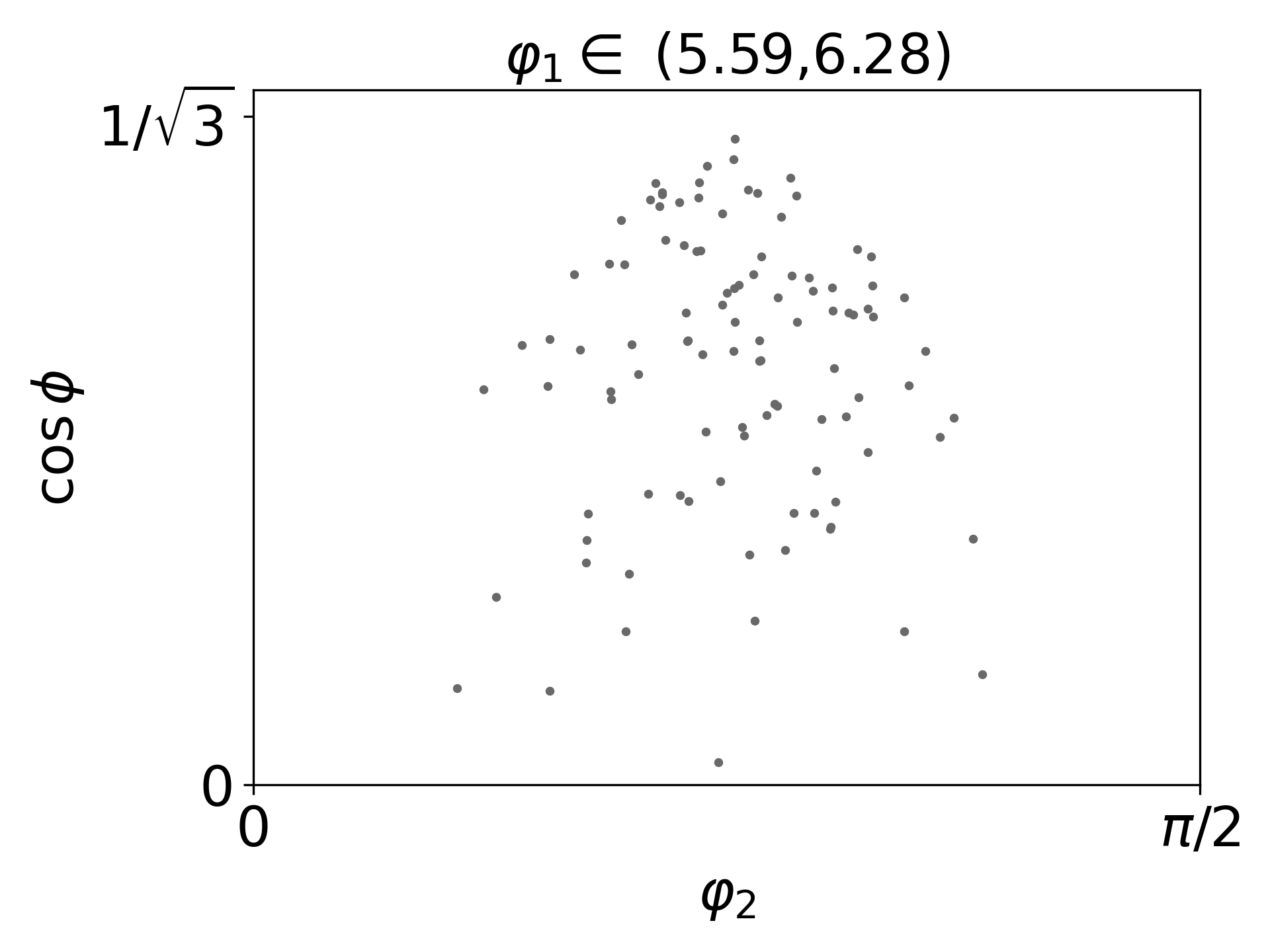
Figure 4: Transformed Euler angles for the NiTi dataset: Scatter plots of pairs $(\cos\phi,\varphi_{2})$ with the corresponding $\varphi_{1}$ in one of nine intervals as stated on the top of each plot.

Figure 3(b) shows the relationship between the inner product (7) and the disorientation angle (6) for the data. In comparison to Figure 3(a), a slightly stronger negative correlation takes place as the Spearman rank correlation coefficient is $-0.991$ and the disorientation distribution is shifted to the left.

4   Models

In continuation of the model of random Laguerre tessellation distribution from [28], we now look for a suitable model for the conditional distribution of the orientations $\mathbf{g}_{n}$ given the Laguerre tessellation $\mathbf{C}_{n}$. We start in Section 4.1 with a semiparametric model for the Euler angles, where its probability density function (pdf) is fully specified. Then we expand on this model in Section 4.2 by introducing three parametric models which account for the interaction between orientations of neighbouring grains. Estimation of the parameters of these three models is deferred to Section 5.

4.1   A semiparametric model for the Euler angles

In this section we assume for simplicity that $\mathbf{g}_{n}$ is independent of $\mathbf{C}_{n}$ and $g_{1},\dots,g_{n}$ are independent and identically distributed. Hence we are left with specifying a model for a single grain with Euler angles $(\varphi_{1},\phi,\varphi_{2})$ within the fundamental zone $F$.

Figure 4 indicates that $\varphi_{1}$ and $(\phi,\varphi_{2})$ of the NiTi dataset are independent, and also that

$$\varphi_{2} \phi [\arcsin\cot\phi,\arccos\cot\phi]$$ conditioned on is uniformly distributed on , (8)

where the endpoints of this interval are obtained by considering (3) and solving the equation $\phi=\phi_{0}(\varphi_{2})$ with respect to $\varphi_{2}$. Moreover, Figure 5 shows histograms of $\varphi_{1}$ and $\cos\phi$ based on the NiTi dataset. Figure 5(a) suggests that $\varphi_{1}$ follows a multimodal distribution which we do not recognize as a known distribution. Therefore, we use periodic cubic B-splines (with period $2\pi$) [6] to estimate the pdf of $\varphi_{1}$; this estimate is denoted $f_{1}(\varphi_{1})$. Furthermore, Figure 5(b) indicates that $\sqrt{3}\cos\phi$ follows a beta distribution with shape parameters $\alpha>0$ and $\beta>0$. Replacing $(\alpha,\beta)$ by its maximum likelihood estimate $(11.79,2.33)$ and using (8), we obtain an estimated pdf of $(\phi,\varphi_{2})$ which is denoted $f_{2}(\phi,\varphi_{2})$. Thus,

$$f_{\text{s}}(g)=f_{1}(\varphi_{1})f_{2}(\phi,\varphi_{2}),\quad(\varphi_{1},\phi,\varphi_{2})\in F$$ (9)

is the estimated pdf of $(\varphi_{1},\phi,\varphi_{2})$ (here the subscript ‘s’ refers to that a single orientation is considered).

In summary, our (estimated) semiparametric model is given by that $\mathbf{g}_{n}$ and $\mathbf{C}_{n}$ are independent, where $\mathbf{g}_{n}$ has pdf

$$f_{\text{noint}}(\mathbf{g}_{n})=\prod_{i=1}^{n}f_{\text{s}}(g_{i})$$ (10)

(‘noint’ in the subscript refers to ‘no interaction’).

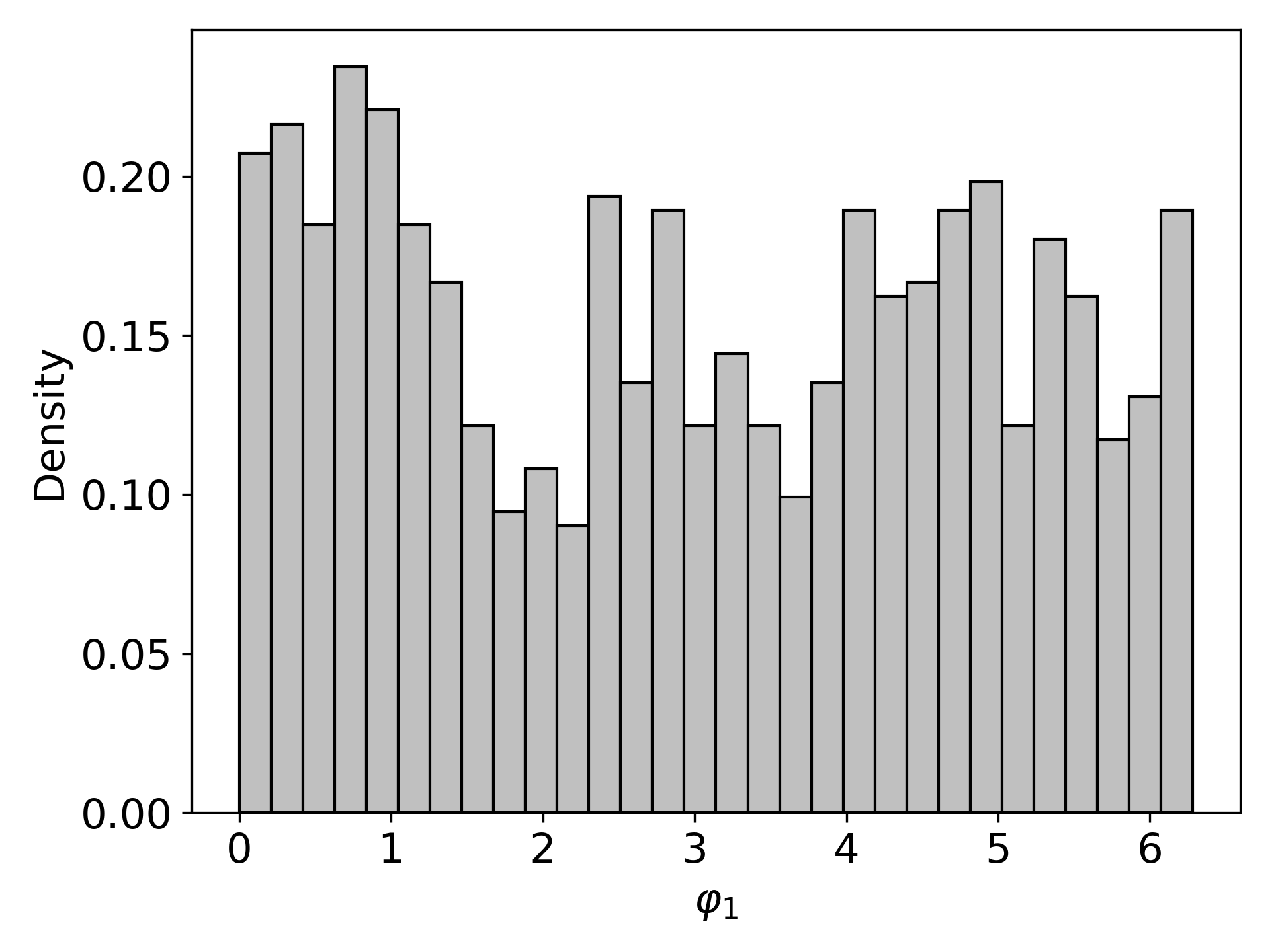
(a)

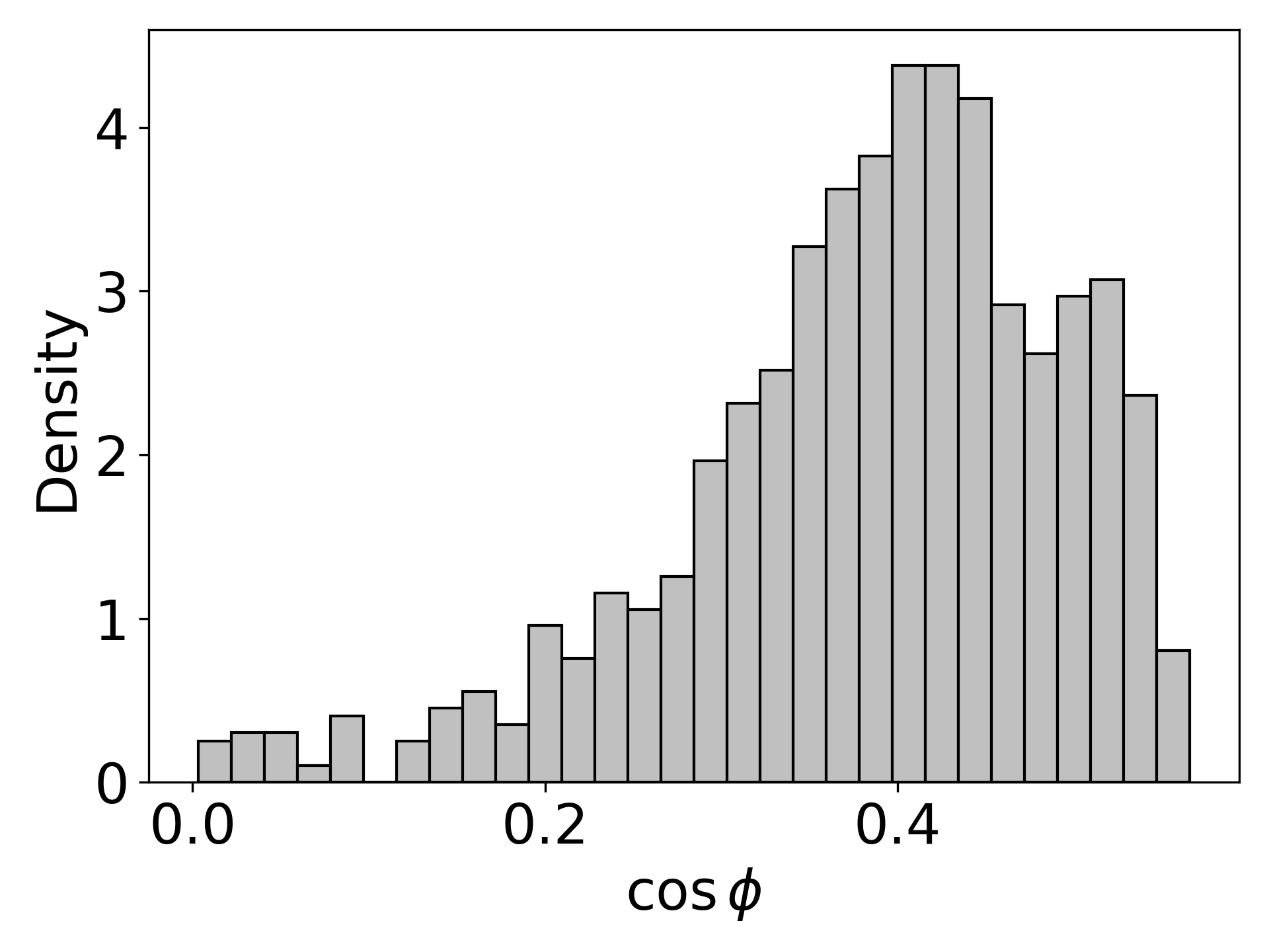
(b)

Figure 5: Histograms of (a) the first Euler angle $\varphi_{1}$ and (b) $\cos\phi$ within the transformed fundamental zone (3) for NiTi dataset.

4.2   Models with interaction terms

Since the presence of a dependence between $\mathbf{g}_{n}$ and $\mathbf{C}_{n}$ was revealed in [23], an extension of the model (10) is needed. Below we therefore consider three closely related models which incorporate pairwise interaction between orientations of neighbouring grains and which only differ in the choice of certain weights.

The general form of the pairwise interaction pdf we consider is

$$f_{\text{int,w}}(\mathbf{g}_{n}\mid\mathbf{C}_{n})\propto\left(\prod_{i=1}^{n}f_{\text{s}}(g_{i})\right)\exp\bigg{\{}\theta\sum_{i\sim j}w_{ij}\operatorname*{inn}(g_{i},g_{j})\bigg{\}},$$ (11)

where $i\sim j$ means that $C_{i}$ and $C_{j}$ are neighbours (that is, they share a face in the Laguerre tessellation), the sum $\sum_{i\sim j}\cdots$ is over all such neighbouring pairs, $w$ is the collection of all weights $w_{ij}$ with $i\sim j$ and $\theta$ is a real unknown parameter. The right-hand side in (11) is an unnormalized density where the normalizing constant depends on both $\mathbf{C}_{n}$ and $\theta$. Moreover, the weights are assumed to be of three types $w^{(k)}$, $k=0,1,2$:

$$w_{ij}^{(0)}=1,\quad w_{ij}^{(1)}=\min\left(\frac{|C_{i}|_{3}}{|C_{j}|_{3}},\frac{|C_{j}|_{3}}{|C_{i}|_{3}}\right),\quad w_{ij}^{(2)}=\frac{|C_{i}\cap C_{j}|_{2}}{\min\left(|C_{i}|_{2},|C_{j}|_{2}\right)},$$

where for a Borel set $C\subseteq W$, $|C|_{2}$ and $|C|_{3}$ denote the surface area and volume of $C$, respectively. Thus in (11), for $w=w^{(k)}$,

• there is no weighting if $k=0$;

• the weight can range from 0 to 1 when $k>0$;

• if $k=1$, high weights mean similar volumes;

• if $k=2$, the weight specifies how large the surface area of the common face is as compared to the smaller surface area of the two grains.

The weight $w^{(2)}$ may be understood by considering first the numerator $|C_{i}\cap C_{j}|_{2}$ and then the denominator $\min\left(|C_{i}|_{2},|C_{j}|_{2}\right)$ which is added in order to obtain a dimensionless quantity. Clearly, $w^{(0)}$ and $w^{(1)}$ are also dimensionless.

Other kinds of interaction models could of course be considered. Furthermore, the inner product in (11) can be replaced with the disorientation angle. However, since the disorientation angle and the inner product for the orientations of two neighbouring grains are strongly negatively correlated (cf. Figure 3(b)), the behaviour of such a model would not be much different. Moreover, simulation under the model with disorientation angle is much more time-consuming because we have to consider all 24 elements of $\mathcal{O}$ when calculating the disorientation angle.

5   Methods

This section describes the methods used for the analysis of the NiTi dataset from Section 3.

Our first model has already been fitted in Section 4.1, but for the three models in Section 4.2 it remains to estimate the parameter $\theta$. Recall that the general form of the pdf for the three models is given by (11). This pdf depends on an intractable normalizing constant $c(\theta,\mathbf{C}_{n})$ given by an integral with respect to $n$-fold product measure of $\mu_{F}$, cf. Section 2.2. Therefore we consider a pseudolikelihood function [2] for $\theta$ which does not depend on $c(\theta,\mathbf{C}_{n})$ as it is given by the product of the $n$ full conditional densities for the $n$ orientations. For $i=1,\dots,n$, denote $(\mathbf{g}_{n})_{-i}$ the vector obtained from $\mathbf{g}_{n}$ by omitting the $i$th orientation $g_{i}$, and $f_{i\theta}(\cdot\mid(\mathbf{g}_{n})_{-i},\mathbf{C}_{n})$ the conditional pdf for the $i$th orientation given the rest. By (11),

$$f_{i\theta}(g_{i}\mid(\mathbf{g}_{n})_{-i},\mathbf{C}_{n})\propto f_{\mathrm{s}}(g_{i})\exp\left\{\theta\sum_{j:\,i\sim j}w_{ij}\operatorname*{inn}(g_{i},g_{j})\right\},$$

where the normalizing constant is

$$c_{i}(\theta,\mathbf{C}_{n})=\int f_{\mathrm{s}}(g_{i})\exp\left\{\theta\sum_{j:\,i\sim j}w_{ij}\operatorname*{inn}(g_{i},g_{j})\right\}\,\mathrm{d}\mu_{F}(g_{i}).$$

Now, the log-pseudolikelihood function for $\theta$ is

$$l(\theta)=\sum_{i=1}^{n}\ln f_{i\theta}(g_{i}\mid(\mathbf{g}_{n})_{-i},\mathbf{C}_{n}).$$

The first and second derivatives of $l(\theta)$ are easily derived and it follows that $l(\theta)$ is a concave function. Hence $l(\theta)$ is easily maximized using the Newton–Raphson method. Since $c_{i}(\theta,\mathbf{C}_{n})$ has to be calculated by numerical methods, approximations of the derivatives $l^{\prime}(\theta)$ and $l^{\prime\prime}(\theta)$ are given in B.

When inspecting each of the four fitted models, it is worth stressing that due to the complexity of the data in hand we do not make any formal hypothesis tests, such as a global envelope test [21], as we admit that these may very well lead to very small $p$-values. On the other hand, we concentrate on comparing how well the empirical distribution of selected orientation characteristics (the orientations themselves as well as those in Section 2.3) agree with the corresponding distributions obtained by simulations under a fitted model. This comparison is done partly by plotting the empirical distribution function for the data and the simulations and partly by calculating mean and standard deviations as detailed in Section 6. Moreover, we compare different fitted models by considering the maximal value of the log-pseudolikelihood function.

It remains to discuss how to make simulations. For the first model in Section 4.1, the orientations are independent and each orientation follows the density $f_{\mathrm{s}}(g)=f_{1}(\varphi_{1})f_{2}(\phi,\varphi_{2})$, cf. (9). We use rejection sampling when simulating from $f_{1}$ and a two-step method for simulation of $(\phi,\phi_{2})\sim f_{2}$: first $\cos\phi$ is sampled from the fitted beta distribution and then $\varphi_{2}$ is sampled from the conditional uniform distribution, cf. (8). For the pairwise interaction models which are given by (11), we use a Metropolis-within-Gibbs algorithm with a cyclic updating scheme which updates the orientations from one end to the other (a so-called sweep, see [7, Section 4.3.3]). Here, when updating the $i$th orientation, if $g_{i,\mathrm{old}}$ and $(\mathbf{g}_{n})_{-i}$ specify the current state of orientations, we propose a new value $g_{i}$ generated from $f_{\mathrm{s}}$ and accept this with probability $\min\{1,H_{i}(g_{i},g_{i,\mathrm{old}},(\mathbf{g}_{n})_{-i})\}$ (otherwise we keep $g_{i,\mathrm{old}}$), where

$$H_{i}(g_{i},g_{i,\mathrm{old}},(\mathbf{g}_{n})_{-i})=\exp\left\{\theta\sum_{j:\,i\sim j}w_{ij}\left[\operatorname*{inn}(g_{i},g_{j})-\operatorname*{inn}(g_{i,\mathrm{old}},g_{j})\right]\right\}$$

is the Hastings ratio.

6   Analysis of the NiTi dataset

We now use our methodology for analysing the NiTi dataset introduced in Section 3. Below we first describe Table 1 and Figure 6 and second comment on our findings.

Table 1: Empirical results for the NiTi dataset and simulated results under fitted models. First row: The maximum pseudolikelihood estimate of $\theta$ for the three pairwise interaction models. Second row: The corresponding values for the maximized log-pseudolikelihood function. The remaining rows: Numerical results for mean values and standard deviations of various orientation characteristics based on Monte Carlo estimates (first to fourth columns) and the NiTi dataset (last column).

	$f_{\text{noint}}$	$f_{\text{int},w^{(0)}}$	$f_{\text{int},w^{(1)}}$	$f_{\text{int},w^{(2)}}$	data
$\hat{\theta}$	–	$0.17$	$0.29$	$2.82$	–
$l(\hat{\theta})$	–	$-243.90$	$-257.06$	$\mathbf{-240.32}$	–
tilt [mean]	$0.953$	$\mathbf{0.959}$	$0.958$	$\mathbf{0.959}$	$0.959$
tilt [sd]	$0.048$	$\mathbf{0.043}$	$0.044$	$\mathbf{0.043}$	$0.039$
$\operatorname*{dis}$ [mean]	$24.257$	$35.213$	$35.846$	$\mathbf{35.698}$	$35.498$
$\operatorname*{dis}$ [sd]	$14.692$	$\mathbf{13.660}$	$13.583$	$13.608$	$13.889$
$\operatorname*{inn}$ [mean]	$0.565$	$0.190$	$0.167$	$\mathbf{0.173}$	$0.181$
$\operatorname*{inn}$ [sd]	$0.517$	$\mathbf{0.489}$	$0.486$	$0.487$	$0.496$
$\hat{d}$	$0.634$	$\mathbf{1.061}$	$1.071$	$1.068$	$1.061$

$f_{\text{noint}}$	$f_{\text{int},w^{(0)}}$	$f_{\text{int},w^{(1)}}$	$f_{\text{int},w^{(2)}}$

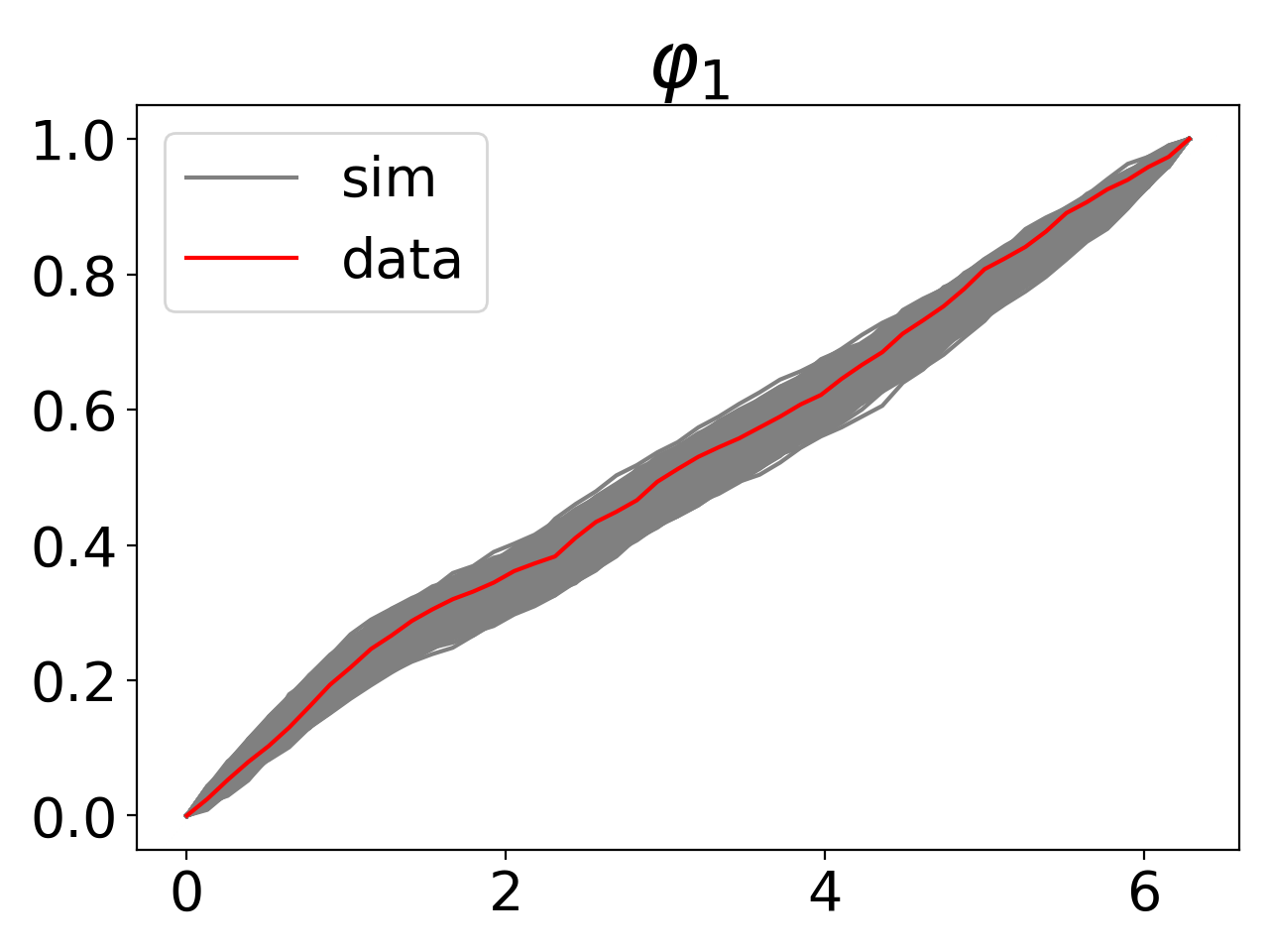
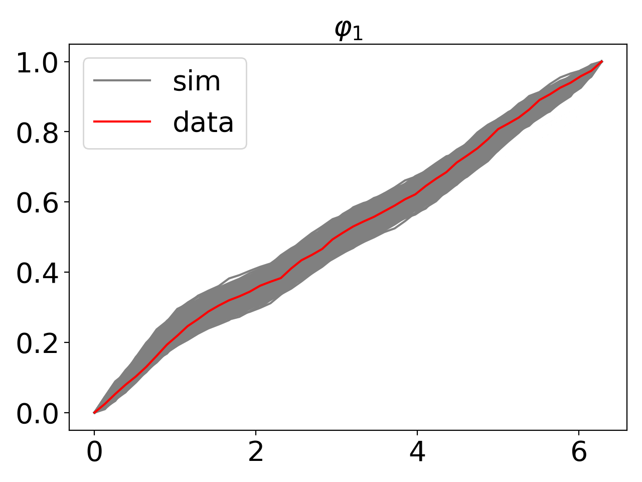
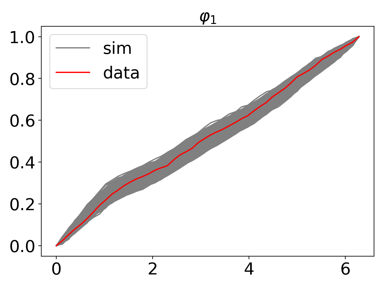
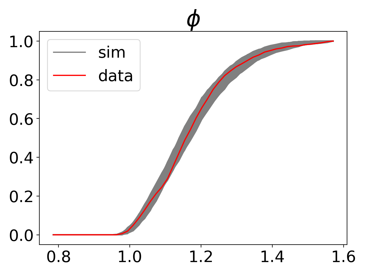
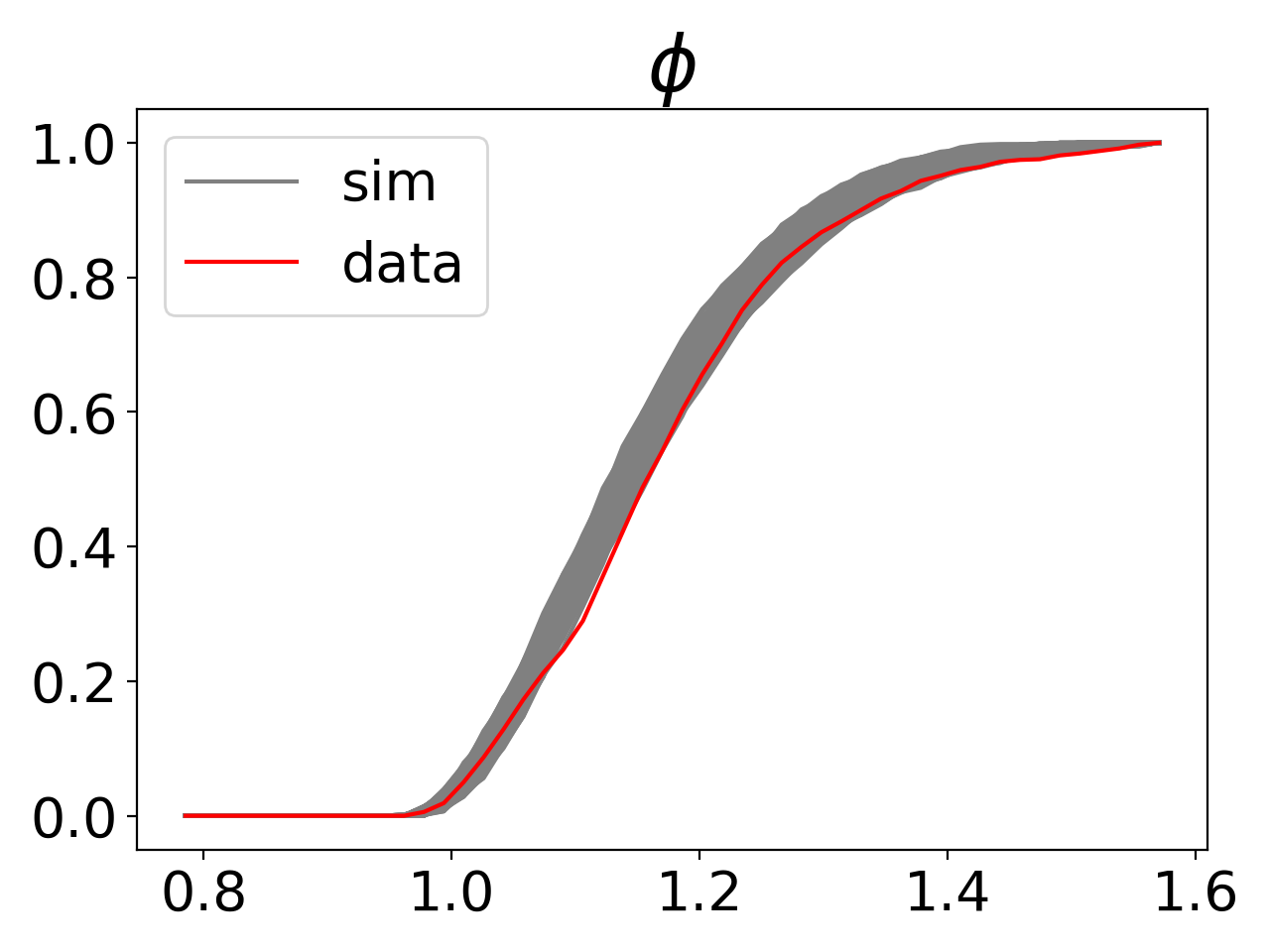
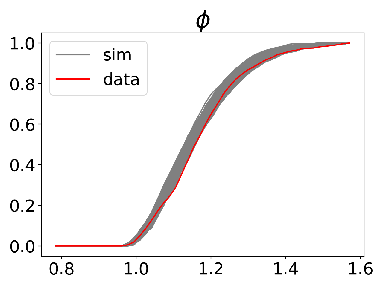
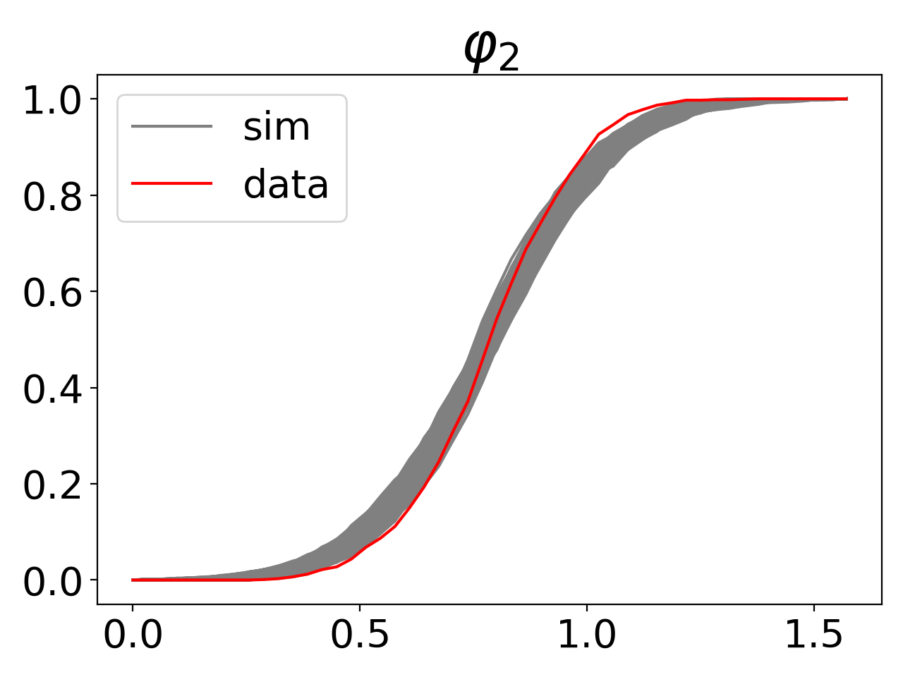
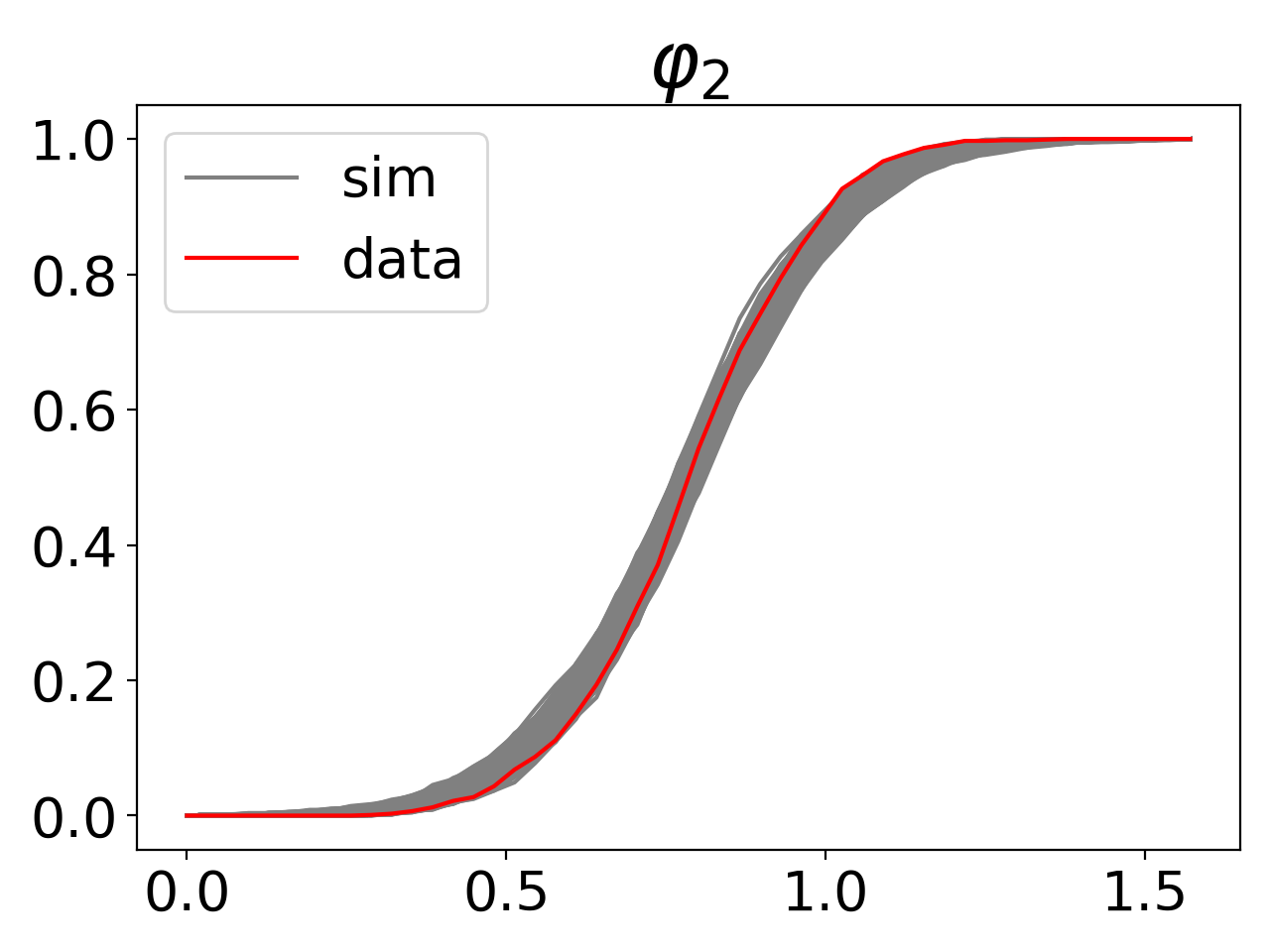
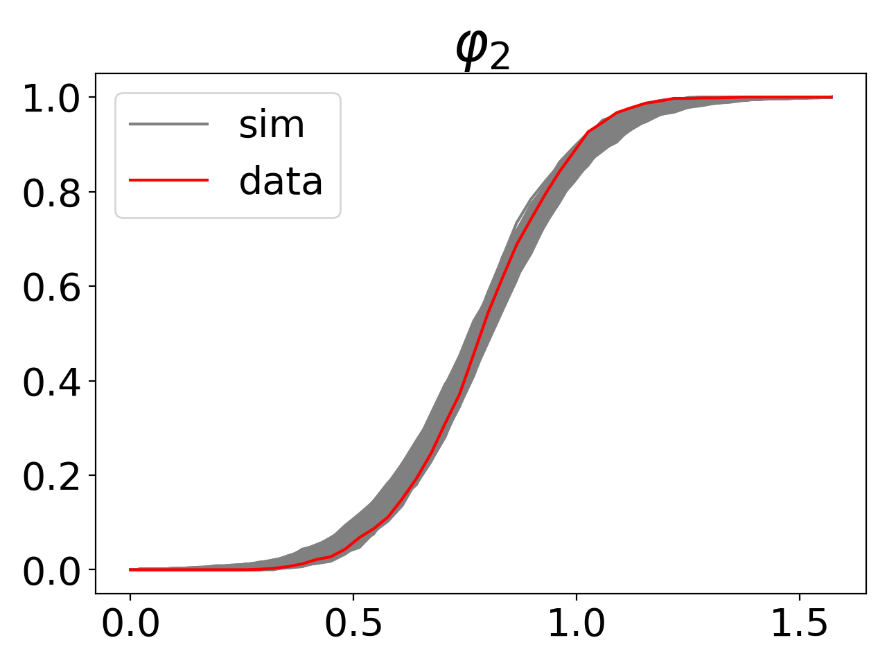
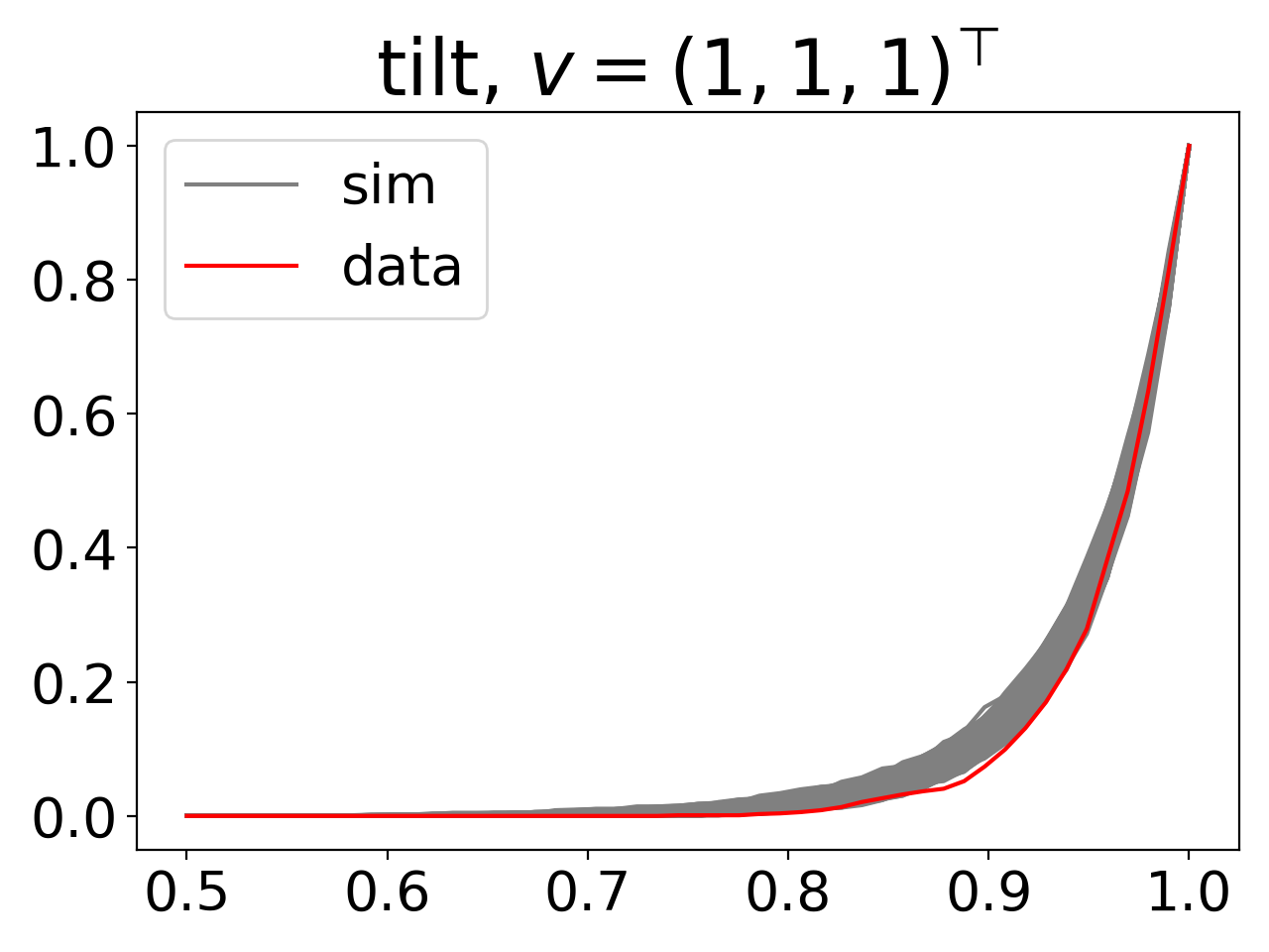
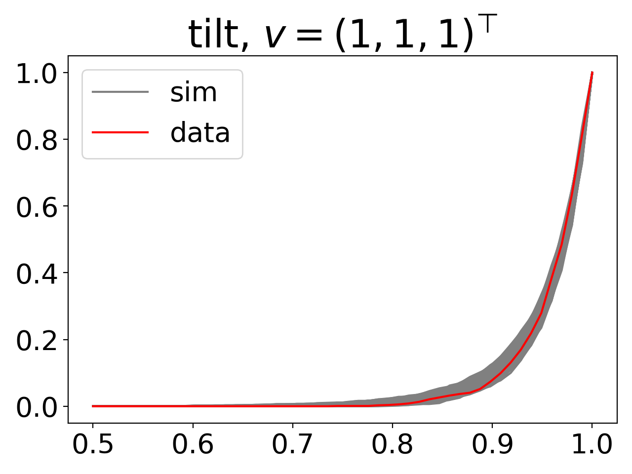
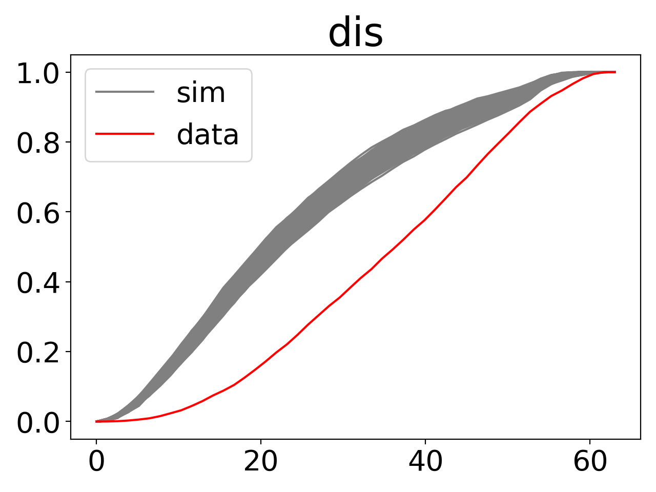
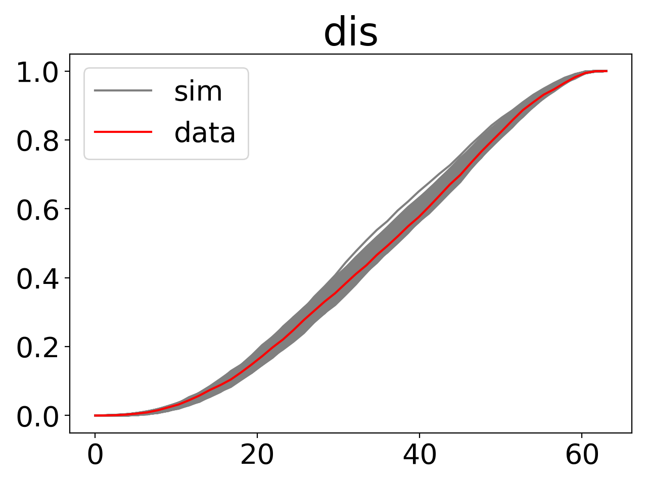
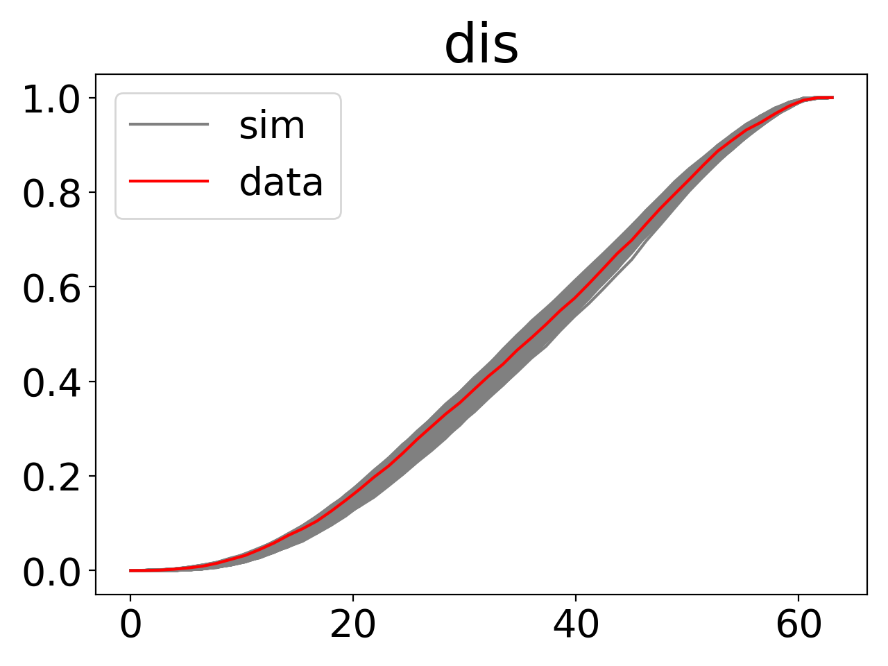
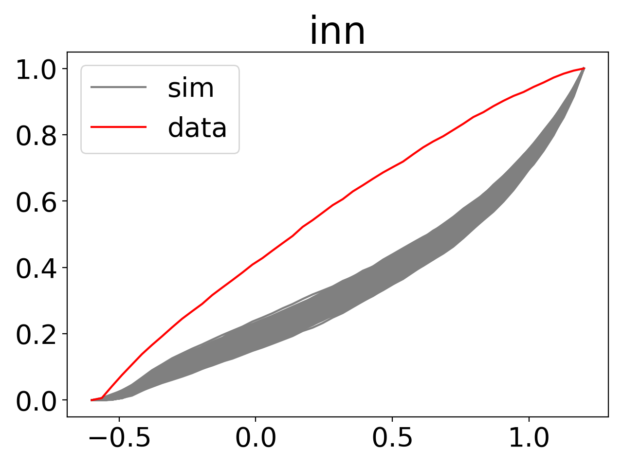
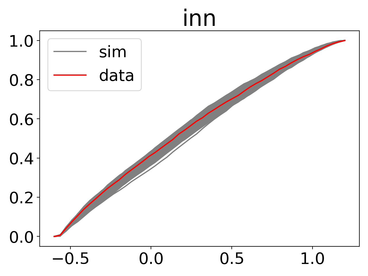
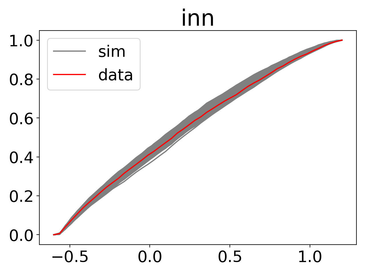
Figure 6: Empirical distribution functions of various orientation characteristics based on the data (red curves) and $5\,000$ simulations (grey curves) under each of the fitted models with densities $f_{\text{noint}}$ (first column), $f_{\text{int},w^{(0)}}$ (second column), $f_{\text{int},w^{(1)}}$ (third column) and $f_{\text{int},w^{(2)}}$ (last column).

Table 1 summarizes numerical results based on partly pseudolikelihood estimation (first and second rows) and partly selected orientation characteristics (remaining rows) given by the tilt with choice $v=(1,1,1)^{\top}$, disorientation angle, inner product and sample dispersion, cf. Section 2.3. The second row shows the values of the maximized log-pseudolikelihood function for the three pairwise interaction models, where the largest value is highlighted. The last column shows the results for the data and the first four columns concern the results obtained from $5\,000$ simulations under each of the four fitted models in Section 4. The closest values to the last column are highlighted. When simulating from models $f_{\text{int},w^{(k)}}$, $k=0,1,2$, $1\,000$ sweeps from the Metropolis-within-Gibbs algorithm were sufficient (here, we omit the time series plots for various statistics which we considered).

Figure 6 shows the empirical distribution functions of various orientation characteristics as calculated from the data and $5\,000$ simulations under each of the four fitted models in Section 4. The figure may be divided into the first four rows, which concern the samples of orientations, and the last two rows, which concern the samples obtained by considering all pairs of neighbouring orientations.

Regarding the first model with pdf $f_{\text{noint}}$ (see (10)), considering the first column in Figure 6, we see that the two first Euler angles are fitted well, but less so for the third Euler angle and the tilt. Moreover, the distribution functions of the disorientation angle and the inner product characteristic are far from the real data.

For the pairwise interaction model with weight $w^{(0)}$ (and having pdf $f_{\text{int},w^{(0)}}$, cf. (11)), we compare with the results above for the first model as well as the data. Comparing the two first columns in Figure 6, we see not much difference with respect to the two first Euler angles, but there is a slight improvement for the third Euler angle and the tilt, and as expected a pronounced improvement for the disorientation angle and the inner product characteristic. Moreover, all the values of the orientation characteristics in Table 1 are now closer to the corresponding values for the data.

For the pairwise interaction model with weight $w^{(1)}$ (and having pdf $f_{\text{int},w^{(1)}}$), we see the following when comparing with the data and the two models above. Based on the third column in Figure 6, in comparison to the first model (the first column), we again observe a slight improvement regarding the Euler angles and the tilt, as well as an improvement regarding the disorientation angle and the inner product characteristic. On the other hand, with respect to the pairwise interaction model with weight $w^{(0)}$ (the second column) we do not observe any change. Further, considering next Table 1, all the values of the orientation characteristics are closer to the corresponding values for the data than for the first model, but farther away from the data than for the pairwise interaction model with weight $w^{(0)}$. In addition, the value of the maximized log-pseudolikelihood function is lower.

Finally, we compare the pairwise interaction model with weight $w^{(2)}$ (and having pdf $f_{\text{int},w^{(2)}}$) with the data and the three models above. Considering the last column in Figure 6, in comparison to the first model we observe again a slight improvement with respect to the Euler angles and the tilt, as well as an improvement with respect to the disorientation angle and the inner product characteristic. However, we do not observe any change with respect to the pairwise interaction models with weights $w^{(0)}$ and $w^{(1)}$. Furthermore, all the orientation characteristics in Table 1 are closer to the data in comparison to the first model and to the pairwise interaction model with weight $w^{(1)}$. On the other hand, some of the values are farther away from the data than for the pairwise interaction model with weight $w^{(0)}$ and some of the values are closer to the data. The values for the tilt are the same. Moreover, the value of the maximized log-pseudolikelihood function is now the largest.

In conclusion, we do not obtain a clear picture from Figure 6 except that one of the pairwise interaction models should be preferred, while the results in Table 1 show that one of the pairwise interaction models with weight $w^{(0)}$ or $w^{(2)}$ should be preferred.

Appendix A Transversal for a cubic lattice structure

In the case of cubic crystal symmetry, the subgroup $\mathcal{O}$ has 24 elements and thus each equivalence class of $\mathrm{SO}(3)$ contains 24 symmetrically equivalent orientations. A transversal is obtained by taking exactly one representative from each equivalence class. When dealing with Euler angles $\left(\varphi_{1},\,\phi,\,\varphi_{2}\right)$, a particular partition of $[0,2\pi)\times[0,\pi]\times[0,2\pi)$ into 24 subsets (representing transversals) is described in [10, Section 2.6.2] and [12, Section 3.4]. However, this description lacks the specification of the boundaries of the subsets. The subset called III in [10, Section 2.6.2] and [12, Section 3.4] corresponds to the fundamental zone $F$ defined by (1) in Section 2.1. It is not difficult to see that $F$ is not a transversal for $\mathcal{O}$ in $\mathrm{SO}(3)$. For example, orientations $G_{1}$, $G_{2}$ given by Euler angles $(0,\pi/2,0),(\pi,\pi/2,0)\in F$, respectively, are equivalent because $G_{2}=SG_{1}$ for some $S\in\mathcal{O}$. All symmetries belonging to $\mathcal{O}$ could be described by Euler angles which are multiples of $\pi/2$. In particular, $S$ is represented by $(\pi,\pi,0)$. We use the notation $(\pi,\pi/2,0)=(\pi,\pi,0)(0,\pi/2,0)$ to rewrite the relation $G_{2}=SG_{1}$.

By thoroughly investigating the boundary of $F$ we find out which orientations to exclude from $F$ in order to obtain a transversal. In this way, we get that a transversal $F_{0}$ contained in $F$ could be taken as

$$F_{0}=F\setminus(F_{1}\cup F_{2}\cup F_{3}\cup F_{4}),$$

where

$$F_{1} =\{(\varphi_{1},\phi_{0}(\varphi_{2}),\varphi_{2})\mid\varphi_{1}\in[0,2\pi),\varphi_{2}\in(\pi/4,\pi/2)\},$$

$$F_{2} =\{(\varphi_{1},\pi/2,\varphi_{2})\mid\varphi_{1}\in[\pi,2\pi),\varphi_{2}\in(0,\pi/2)\},$$

$$F_{3} =\{(\varphi_{1},\phi_{0}(\pi/4),\pi/4)\mid\varphi_{1}\in[2\pi/3,2\pi)\},$$

$$F_{4} =\{(\varphi_{1},\pi/2,0)\mid\varphi_{1}\in[\pi/2,2\pi)\}.$$

Note that $F$ and $F_{0}$ have the same interiors and $\mu(F\setminus F_{0})=0$. The explanation of the form of individual sets that are excluded from $F$ follows below. For this purpose it is useful to observe the contour line of $F$ with given $\varphi_{1}$ shown in Figure 7.

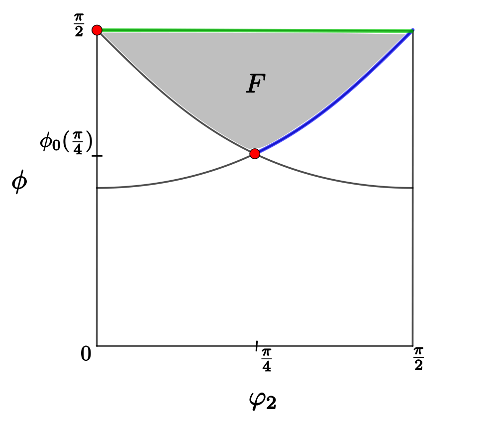
Figure 7: A cross-section of the fundamental zone $F$ given by (1). The sets of points that need to be considered in order to get the transversal $F_{0}$ are highlighted.

First consider $(\varphi_{1},\phi_{0}(\varphi_{2}),\varphi_{2})$ with $\varphi_{2}\in(0,\pi/4)$. This orientation is equivalent to$(\tilde{\varphi_{1}},\phi_{0}(\varphi_{2}),\pi/2-\varphi_{2})$ with $\tilde{\varphi_{1}}$ possibly different from $\varphi_{1}$. Therefore, we restrict only to $\varphi_{2}\in(0,\pi/4)$ in $F_{0}$ and remove the set $F_{1}$, where $\varphi_{2}\in(\pi/4,\pi/2)$, depicted by a blue colour in Figure 7. The symmetry that transforms $(\varphi_{1},\phi_{0}(\varphi_{2}),\varphi_{2})$ to $(\tilde{\varphi_{1}},\phi_{0}(\varphi_{2}),\pi/2-\varphi_{2})\in F_{1}$ is given by Euler angles $(\pi/2,\pi/2,0)$. It means that

$$(\tilde{\varphi_{1}},\phi_{0}(\varphi_{2}),\pi/2-\varphi_{2})=(\pi/2,\pi/2,0)(\varphi_{1},\phi_{0}(\varphi_{2}),\varphi_{2}) \varphi_{2}\in(0,\pi/4)$$ for .

The form of $F_{2}$ (green segment in Figure 7) follows from the relation

$$(\varphi_{1}+\pi,\pi/2,\pi/2-\varphi_{2})=(\pi/2,\pi,0)(\varphi_{1},\pi/2,\varphi_{2}) \varphi_{1}\in[0,\pi) \varphi_{2}\in(0,\pi/2)$$ for and .

It means that for $\phi=\pi/2$ we exclude one half of the $\varphi_{1}$ values from $F$.

If $\phi=\phi_{0}(\pi/4)=\arccos(1/\sqrt{3})$ and $\varphi_{2}=\pi/4$ (right bottom red dot in Figure 7) we exclude two thirds of the $\varphi_{1}$-range (set $F_{3}$) because

$$(\varphi_{1}+2\pi/3,\phi_{0}(\pi/4),\pi/4)=(\pi/2,\pi/2,0)(\varphi_{1},\phi_{0}(\pi/4),\pi/4)$$

and

$$(\varphi_{1}+4\pi/3,\phi_{0}(\pi/4),\pi/4)=(\pi,\pi/2,\pi/2)(\varphi_{1},\phi_{0}(\pi/4),\pi/4)$$

for $\varphi_{1}\in[0,2\pi/3)$.

Finally, similar reasoning applies to the case $\phi=\pi/2$ and $\varphi_{2}=0$ (left upper red dot in Figure 7). Then $(\varphi_{1},\pi/2,0)$ with $\varphi_{1}\in[0,\pi/2)$ is equivalent to $(\varphi_{1}+k\pi/2,\pi/2,0)$, $k=1,2,3$. More specifically, we have

$$(\varphi_{1}+\pi/2,\pi/2,0) =(\pi/2,\pi/2,3\pi/2)(\varphi_{1},\pi/2,0),$$

$$(\varphi_{1}+\pi,\pi/2,0) =(\pi,\pi,0)(\varphi_{1},\pi/2,0),$$

$$(\varphi_{1}+3\pi/2,\pi/2,0) =(3\pi/2,\pi/2,\pi/2)(\varphi_{1},\pi/2,0)$$

for $\varphi_{1}\in[0,\pi/2)$. Any transversal must contain only one of four equivalent orientations $(\varphi_{1}+k\pi/2,\pi/2,0)$, $k=0,1,2,3$. We choose $\varphi_{1}\in[0,\pi/2)$ in $F_{0}$.

Appendix B Derivatives of the log-pseudolikelihood function

The log-pseudolikelihood function in Section 5 is given as

$$l(\theta) =\sum_{i=1}^{n}\ln f_{i\theta}(g_{i}\mid(\mathbf{g}_{n})_{-i},\mathbf{C}_{n})$$

$$=\sum_{i=1}^{n}\ln\left(\frac{1}{c_{i}(\theta,\mathbf{C}_{n})}f_{\rm s}(g_{i})\exp\left\{\theta\sum_{j:\,i\sim j}w_{ij}\operatorname*{inn}(g_{i},g_{j})\right\}\right)$$

$$=\sum_{i=1}^{n}\left(-\ln c_{i}(\theta,\mathbf{C}_{n})+\ln f_{\rm s}(g_{i})+\theta\sum_{j:\,i\sim j}w_{ij}\operatorname*{inn}(g_{i},g_{j})\right).$$

The first and second derivatives of $l(\theta)$ with respect to the parameter $\theta$ are

$$l^{\prime}(\theta)=\sum_{i=1}^{n}\left(-\frac{c_{i}^{\prime}(\theta,\mathbf{C}_{n})}{c_{i}(\theta,\mathbf{C}_{n})}+\sum_{j:\,i\sim j}w_{ij}\operatorname*{inn}(g_{i},g_{j})\right)$$

and

$$l^{\prime\prime}(\theta)=\sum_{i=1}^{n}\left(\frac{c_{i}^{\prime}(\theta,\mathbf{C}_{n})}{c_{i}(\theta,\mathbf{C}_{n})}\right)^{2}-\sum_{i=1}^{n}\frac{c_{i}^{\prime\prime}(\theta,\mathbf{C}_{n})}{c_{i}(\theta,\mathbf{C}_{n})}.$$

Consider $t(F)$ (see Section 2.2) equipped with the measure (4). It is easily seen that $t(F)$ has volume $\pi^{2}/3$. Divide $t(F)$ into $M$ equally large cells with midpoints $\left\{u_{m},\,m=1,\dots,M\right\}$. Denoting $t^{-1}:(\varphi_{1},\eta,\varphi_{2})\mapsto(\varphi_{1},\phi,\varphi_{2})$, we approximate the normalizing constant

$$c_{i}(\theta,\mathbf{C}_{n}) =\int f_{\mathrm{s}}(g)\exp\left\{\theta\sum_{j:\,i\sim j}w_{ij}\operatorname*{inn}(g,g_{j})\right\}\,\mathrm{d}\mu_{F}(g)$$

$$=\int_{t(F)}f_{\mathrm{s}}(t^{-1}(\varphi_{1},\eta,\varphi_{2}))\ \times$$

$$\quad\quad\times\exp\left\{\theta\sum_{j:\,i\sim j}w_{ij}\operatorname*{inn}(t^{-1}(\varphi_{1},\eta,\varphi_{2}),(\varphi_{1j},\phi_{j},\varphi_{2j}))\right\}\,\mathrm{d}(\varphi_{1},\eta,\varphi_{2})$$

$$\approx\frac{\pi^{2}}{3M}\sum_{m=1}^{M}f_{\mathrm{s}}(t^{-1}(u_{m}))\exp\left\{\theta\sum_{j:\,i\sim j}w_{ij}\operatorname*{inn}(t^{-1}(u_{m}),g_{j})\right\}.$$

The approximation of the first and second derivatives of the log-pseudolikelihood function with respect to the parameter $\theta$ are then

$$l^{\prime}(\theta)\approx \sum_{i=1}^{n}\sum_{j:\,i\sim j}w_{ij}\operatorname*{inn}(g_{i},g_{j})$$

$$-\sum_{i=1}^{n}\dfrac{\sum\limits_{m=1}^{M}f_{\mathrm{s}}(t^{-1}(u_{m}))\left(\sum\limits_{j:\,i\sim j}w_{ij}\operatorname*{inn}(t^{-1}(u_{m}),g_{j})\right)\exp\left\{\theta\sum\limits_{j:\,i\sim j}w_{ij}\operatorname*{inn}(t^{-1}(u_{m}),g_{j})\right\}}{\sum\limits_{m=1}^{M}f_{\mathrm{s}}(t^{-1}(u_{m}))\exp\left\{\theta\sum\limits_{j:\,i\sim j}w_{ij}\operatorname*{inn}(t^{-1}(u_{m}),g_{j})\right\}}$$

and

$$l^{\prime\prime}(\theta)\approx \sum\limits_{i=1}^{n}\left(\dfrac{\sum\limits_{m=1}^{M}f_{\mathrm{s}}(t^{-1}(u_{m}))\left(\sum\limits_{j:\,i\sim j}w_{ij}\operatorname*{inn}(t^{-1}(u_{m}),g_{j})\right)\exp\left\{\theta\sum\limits_{j:\,i\sim j}w_{ij}\operatorname*{inn}(t^{-1}(u_{m}),g_{j})\right\}}{\sum\limits_{m=1}^{M}f_{\mathrm{s}}(t^{-1}(u_{m}))\exp\left\{\theta\sum\limits_{j:\,i\sim j}w_{ij}\operatorname*{inn}(t^{-1}(u_{m}),g_{j})\right\}}\right)^{2}$$

$$-\sum_{i=1}^{n}\dfrac{\sum\limits_{m=1}^{M}f_{\mathrm{s}}(t^{-1}(u_{m}))\left(\sum\limits_{j:\,i\sim j}w_{ij}\operatorname*{inn}(t^{-1}(u_{m}),g_{j})\right)^{2}\exp\left\{\theta\sum\limits_{j:\,i\sim j}w_{ij}\operatorname*{inn}(t^{-1}(u_{m}),g_{j})\right\}}{\sum\limits_{m=1}^{M}f_{\mathrm{s}}(t^{-1}(u_{m}))\exp\left\{\theta\sum\limits_{j:\,i\sim j}w_{ij}\operatorname*{inn}(t^{-1}(u_{m}),g_{j})\right\}}.$$

References

- [1] R. Arnold, P. E. Jupp, and H. Schaeben. Statistics of ambiguous rotations. Journal of Multivariate Analysis, 165:73–85, 2018.
- [2] J. Besag. Statistical analysis of non-lattice data. Journal of the Royal Statistical Society: Series D (The Statistician), 24(3):179–195, 1975.
- [3] T. Böhlke, U. U. Haus, and V. Schulze. Crystallographic texture approximation by quadratic programming. Acta Materialia, 54(5):1359–1368, 2006.
- [4] K. G. Van den Boogaart. Statistics for Individual Crystallographic Orientation Measurement. Shaker Verlag, 2002.
- [5] K. G. Van den Boogaart, and R. Hielscher, and J. Prestin, and H. Schaeben. Kernel-based methods for inversion of the Radon transform on SO(3) and their applications to texture analysis. Journal of Computational and Applied Mathematics, 199(1):122–140, 2007.
- [6] C. De Boor. On calculating with B-splines. Journal of Approximation Theory, 6(1):50–62, jul 1972.
- [7] S. Brooks, A. Gelman, G. L. Jones, and X. L. Meng, editors. Handbook of Markov Chain Monte Carlo. CRC Press, 2011.
- [8] J. Ding, S. L. Zhang, Q. Tong, L. S. Wang, X. Huang, K. Song, and S. Q. Lu. The effects of grain boundary misorientation on the mechanical properties and mechanism of plastic deformation of Ni/Ni3Al: A molecular dynamics study. Materials, 13(24):5715, 2020.
- [9] T. D. Downs. Orientation statistics. Biometrika, 59(3):665–676, 1972.
- [10] O. Engler and V. Randle. Introduction to Texture Analysis: Macrotexture, Microtexture, and Orientation Mapping. CRC Press, 2nd edition, 2010.
- [11] A. Haar. Der Massbegriff in der Theorie der kontinuierlichen Gruppen. Annals of Mathematics, 34(1):147–169, 1933.
- [12] J. Hansen, J. Pospiech, and K. Lücke. Tables for Texture Analysis of Cubic Crystals. Springer, 1978.
- [13] L. Heller, I. Karafiátová, L. Petrich, Z. Pawlas, P. Shayanfard, V. Beneš, V. Schmidt, and P. Šittner. Numerical microstructure model of NiTi wire reconstructed from 3D-XRD data. Modelling and Simulation in Materials Science and Engineering, 28(5):055007, 2020.
- [14] I. Karafiátová, Z. Pawlas, and L. Heller. Statistical assessment of stress redistribution in loaded polycrystals. Image Analysis & Stereology, 41(1):25–39, 2022.
- [15] C. G. Khatri and K. V. Mardia. The von Mises-Fisher matrix distribution in orientation statistics. Journal of the Royal Statistical Society: Series B (Methodological), 39(1):95–106, 1977.
- [16] C. Lautensack and S. Zuyev. Random Laguerre tessellations. Advances in Applied Probability, 40(3):630–650, 2008.
- [17] C. A. León, J. C. Massé, and L. P. Rivest. A statistical model for random rotations. Journal of Multivariate Analysis, 97(2):412–430, 2006.
- [18] H. F. Liu, L. Zhang, S. J. Chua, and D. Z. Chi. Crystallographic tilt in GaN-on-Si (111) heterostructures grown by metal–organic chemical vapor deposition. Journal of Materials Science, 49(9):3305–3313, 2014.
- [19] A. Morawiec. Orientations and Rotations. Springer, 2004.
- [20] U. Müller. Symmetry Relationships between Crystal Structures. Oxford University Press, 2013.
- [21] M. Myllymäki, T. Mrkvička, P. Grabarnik, H. Seijo, and U. Hahn. Global envelope tests for spatial processes. Journal of the Royal Statistical Society: Series B (Statistical Methodology), 79:381–404, 2017.
- [22] S. R. Niezgoda, E. A. Magnuson, and J. Glover. Symmetrized Bingham distribution for representing texture: parameter estimation with respect to crystal and sample symmetries. Journal of Applied Crystallography, 49(4):1315–1319, 2016.
- [23] Z. Pawlas, I. Karafiátová, and L. Heller. Random tessellations marked with crystallographic orientations. Spatial Statistics, 39:100469, 2020.
- [24] L. Petrich, J. Staněk, M. Wang, D. Westhoff, L. Heller, P. Šittner, C. E. Krill, V. Beneš, and V. Schmidt. Reconstruction of grains in polycrystalline materials from incomplete data using Laguerre tessellations. Microscopy and Microanalysis, 25(3):743–752, 2019.
- [25] H. Poulsen. Three-Dimensional X-Ray Diffraction Microscopy. Springer, 2004.
- [26] H. Schaeben, F. Bachmann, and J. J. Fundenberger. Construction of weighted crystallographic orientations capturing a given orientation density function. Journal of Material Sciences, 52(4):2077–2090, 2017.
- [27] P. Sedmák, J. Pilch, L. Heller, J. Kopeček, J. Wright, P. Sedlák, M. Frost, and P. Šittner. Grain-resolved analysis of localized deformation in nickel-titanium wire under tensile load. Science, 353(6299):559–562, 2016.
- [28] F. Seitl, J. Møller, and V. Beneš. Fitting three-dimensional Laguerre tessellations by hierarchical marked point process models. Spatial Statistics, 51:100658, 2022.
- [29] J. Staněk, J. Kopeček, P. Král, I. Karafiátová, F. Seitl, and V. Beneš. Comparison of segmentation of 2D and 3D EBSD measurements in polycrystalline materials. Kovové Materiály – Metallic Materials, 58(5):301–319, 2020.
- [30] S. Zaefferer and S. I. Wright. Three-dimensional orientation microscopy by serial sectioning and EBSD-based orientation mapping in a FIB-SEM. In A. J. Schwartz, M. Kumar, B. L. Adams, and D. P. Field, editors, Electron Backscatter Diffraction in Materials Science, pages 109–122. Springer, 2009.