Preliminary Bias Results in Search Engines

Abstract.

This report aims to report my thesis progress so far. My work attempts to show the differences in the perspectives of two search engines, Bing and Google on several selected controversial topics. In this work, we try to make a distinction on the viewpoints of Bing & Google by using sentiment as well as the ranking of the document returned from these two search engines on the same queries, these queries are related mainly to controversial topics. You can find the methods we used with experimental results below.

1. Introduction

The core component of my thesis work and our main goal is to show the existence of bias in search engines (Bing & Google) which is a very strong claim, therefore we started to differentiate the attitudes of these two search engines on some controversial topics. You can find the details of our method with the experimental results we obtained in the following sections after the overview of our unpublished work, effective crowd labelling procedure.

2. Sentiment-wise Comparison of Two Search Engines

Two popular search engines were mainly compared from sentiment perspective by exploiting three different levels of sentiment metrics such as document-level, sentence-level, and aspect-level.. Initially, we computed sentiment scores by using TextBlob as well as the polarity values of the words in a widely used domain-independent lexicon, SentiWordNet (Baccianella et al., 2010). However, obtained values from SentiWordNet were not reasonable and did not reflect the real sentiment of the given document. Therefore, we decided to use only TextBlob for sentiment polarity detection in our experiments.

2.1. Document-level Sentiment Analysis

For document-level analysis, we obtain a sentiment value for each document from TextBlob without any pre-processing step on documents, TextBlob handles the punctuation in itself. This part of the analysis is more coarse-grained relatively to the subsequent parts.

2.2. Sentence-level Sentiment Analysis

Differently from document-level, in sentence-level sentiment analysis we view each document as a pile of sentences. This leads to a more fine-grained analysis; thus in this part, we split the given document into sentences and obtain polarity value for each of its sentences from TextBlob. In order to obtain a sentiment score for the given document, we compute an average sentiment by summing the polarity values of all the sentences and dividing it by the number of sentences in the document. That is to say, from TextBlob’s point of view, each sentence is a document and processed accordingly. For clarification, again we have one polarity value for each document to compare the retrieved document sets of two search engines, although we compute these scores in distinct ways.

2.3. Aspect-level Sentiment Analysis

In addition to document and sentence-level, we also analyzed the documents on aspect-level with the hope that it may convey different type of information that is useful for the comparison of the search engines. In analyzing the documents from the aspect-level perspective, we implemented a Java script on Eclipse environment in order to find dependencies between words. In this script, we read documents, split the documents into sentences and with the help of Stanford NLP Parser (Manning et al., 2014) we obtain relations between words. In this way, grammatically we can have deeper understanding of documents and this additional information is exploited while analyzing the documents in terms of sentiment. As a side note, detailed information about the grammatical relations can be found in the Stanford NLP Parser manual.

In extracting dependencies between words in sentences, we only pay attention to the relations of the controversial topic keywords. We select these keywords for each topic as follows, if the given topic is composed of one word, we use that word as the keyword for the corresponding topic. If the topic contains more than one word, then we tokenize the topic title and all of the tokens are used as the keywords for that topic. Note that in our current dataset, topic titles are composed of at most two words, thus we have to deal with two-keywords case in our dependency analysis differently from the simple case of one-keyword topics. You can find sample relations extracted from the one-keyword controversial queries abortion and brexit in Table 1. For two-keywords queries, we obtain dependencies for both of the keywords in the given topic and use all of these dependencies for the analysis. You can find sample relations extracted from the two-keywords controversial query gay marriage in Table 2.

While extracting relations between words, initially we find keyword/s for the given topic, then we merely extract the relations of those keyword/s as mentioned above. Apart from this, we obtain the relations between keywords and only sentiment-baring words i.e., nouns, adjectives, adverbs, verbs. This is stemmed from the fact that we use dependency information for sentiment analysis and non sentiment-baring words will not be useful in our analyses. After getting relations from the parser, we will compute the sentiment score of the words that have grammatical relations with the keywords of the given topic. Sentiment polarities are computed by using TextBlob for all the related words in a document, then we compute an average sentiment score of each document for comparison.

Word-Relation-Keyword
demand - nmod:on - abortion
illegal - nsubj - abortion
laws - compound - abortion
ban - dobj - abortion
restrict - dobj - abortion
negotiations - compound - brexit
bill - compound - brexit
risk - nmod:of - brexit
chaotic - amod - brexit
doubts - compound - brexit

Table 1. Sample Dependencies of Abortion & Brexit

Word-Relation-Keyword
rights - amod - gay
community - amod - gay
activist - amod - gay
fans - amod - gay
nice - amod - gay
legalizing - dobj - marriage
support - nmod:for - marriage
recognize - dobj - marriage
outlaw - dobj - marriage
opposed - dobj - marriage

Table 2. Sample Dependencies of Gay Marriage

3. Experimental Results

3.1. Dataset

In order to observe remarkable differences between the retrieval results of two popular search engines, we selected 15 controversial topics from the website of https://www.procon.org/. We collected data using news API of the corresponding search engines: Bing and Google. With the aim of retrieving more documents related to each topic, we extended the query set by using Google Trends. Then, we implemented scripts on python to automate the crawling process with the API keys of the search engines.

For each query sent to the search engine, we crawled the first 10 documents returned from that search engine. The dataset is composed of 2560 documents in total for one search engine. Topic distribution of the crawled dataset is displayed in Table 3. In the table, one can see that there are 200 documents crawled for the controversial query of abortion, this means that we have 20 extended queries for this specific topic since we use only the first 10 documents retrieved from the corresponding search engine. We note that the data collection process was fulfilled in a controlled environment such that the same queries were sent to the search engines almost at the same moment since the documents to be retrieved may vary by time.

Topic	# of documents
Abortion	200
Animal Testing	80
Assisted Suicide	80
Brexit	180
Climate Change	350
Gay Marriage	220
Gun Control	260
Medical Marijuana	130
Minimum Wage	220
Obamacare	120
Prostitution	70
Syrian Refugees	130
Transgender Military	80
Travel Ban	140
Trump	300

Table 3. Controversial Topic Distributions

3.2. Evaluation Framework

In evaluating two search engines, our aim is to compare these two search engines on conservative/liberal perspective towards a given controversial topic. For comparison, we utilize TextBlob sentiment scores at three different levels , document, sentence, and aspect-level.

In order to make a consistent comparison among all controversial topics, one needs to think about the connection between the semantic orientation and the perspective of the given documents on the scope of their controversial topics. For instance, if a document has a positive sentiment score and its controversial topic is abortion, then the document’s perspective tends to be more liberal, whereas if a document shows a negative attitude towards brexit, similarly its perspective would be more close to liberal. This is because of the fact that the underlying perspective of a document on conservative/liberal axis in our evaluation scheme does not only depend on its semantic orientation but also on the corresponding controversial topic. For this reason, after obtaining polarity values at three different levels via TextBlob, we transformed these values for some of the controversial topics in order to make a consistent comparison for all controversial topics. In order to fulfill the transformation task, the polarity values were simply multiplied by -1 for animal testing, brexit, minimum wage, travel ban, and trump.

In our evaluation scheme, we used two metrics and computed these at three different levels, document, sentence, and aspect-level. As the first metric, sentiment scores obtained from TextBlob were used after the transformation process as mentioned above, if necessary. Secondly, we proposed a new metric that combines rank and sentiment information and takes into account both of these for comparison. Also for the second metric, we used transformed sentiment scores to provide a consistent perspective analysis, instead of the actual polarity values obtained from TextBlob.

3.2.1. Sentiment Polarity Metric

Our first metric compares the two search engines by purely using sentiment scores returned from TextBlob and the range for polarity values is [-1, 1]. We obtained sentiment scores for documents, sentences, and aspects, then computed an average polarity value as mentioned in the previous section for each document by exploiting document, sentence, and aspect-level sentiment values separately. That means that we only care about document sentiment scores for comparison purposes, yet by computing these document scores in three different levels of sentiment analysis then transforming some of these polarity values if needed. You can find the table of mean of mean average sentiment scores in Table 4 and comparison plot of two search engines in terms of mean avg polarity scores in Figure 1.

Sentiment-level	Bing	Google
Document-level	0.0260	0.0241
Sentence-level	0.0195	0.0178
Aspect-level	-0.0018	0.0001

Table 4. Mean of Mean Average Sentiment Scores over All Controversial Topics

Sentiment-level	Bing	Google
Document-level	0.7845	0.7916
Sentence-level	0.7821	0.7967
Aspect-level	0.6099	0.5234

Table 5. Mean Average NDCG-Senti Scores over All Controversial Topics

Dataset	p-value	Is Statistically Significant?
DOCLevel_MeanAvgScore	0.9515	NO
SENTLevel_MeanAvgScore	0.9441	NO
ASPLevel_MeanAvgScore	0.3775	NO
DOCLevel_AvgNDCGScore	0.6225	NO
SENTLevel_AvgNDCGScore	0.2562	NO
ASPLevel_AvgNDCGScore	0.1841	NO

Table 6. Two-tail t-test p-values Over All Controversial
Topics

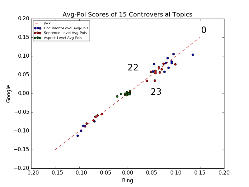
Figure 1. Mean Avg-Pol Scores of 15 Controversial Topics

3.2.2. NDCG-Senti Metric

In addition to the sentiment polarity metric, we also needed a more informative metric that will be convenient to compare particularly the retrieved document sets of two search engines. For this reason, we introduced a new metric, NDCG-Senti that blends ranking and sentiment information, which is a variant of commonly used NDCG metric. We utilized the traditional formula of NDCG denoted in NDCG-FORMULA. For our ranking-sentiment metric NDCG-Senti, we replaced relevance score $rel_{i}$ with sentiment score $pol_{i}$ in the formula.

With a slight modification in the traditional formula of NDCG, we came up with a modified NDCG scoring function which also takes document rank into consideration while comparing document sets of search engines. However, there is still one more issue in the computation of transformed NDCG function that relevance grades in the traditional NDCG metric are always positive, whereas the real sentiment values as well as the transformed ones become negative since the polarity values obtained from TextBlob lie between -1 and 1. Note that the polarity values of documents were firstly transformed and then they were used for the computation of this second metric. In short, we computed NDCG-Senti scores with transformed and subsequently normalized sentiment scores of TextBlob. The normalization was applied as follows: Transformed document polarity values of each query were normalized to the range of [0,1], then our new metric was obtained by using the non-negative sentiment polarities in each query.

In order to get rid of the negative values, we utilize min-max normalization technique to map the polarities onto the range of [0, 1]. For each query, there are 10 transformed sentiment polarities of the documents returned from each search engine. We compute a minimum and a maximum value from these polarity values of the document set of each query. Then, we normalize the polarity values and obtain non-negative scores for the given set of documents. Subsequently, we compute a NDCG-Senti score for the given set of documents with transformed sentiment polarities. In other words, we compute different min-max value pairs for each document set and normalize the polarity values for each query separately. Then we computed an average NDCG-Senti score for each controversial topic by using the NDCG-Senti score of each query in the corresponding topic. You can find the table of mean average NDCG-Senti scores in Table 5 and the comparison plot of two search engines in terms of average NDCG-Senti scores is displayed in Figure 2.

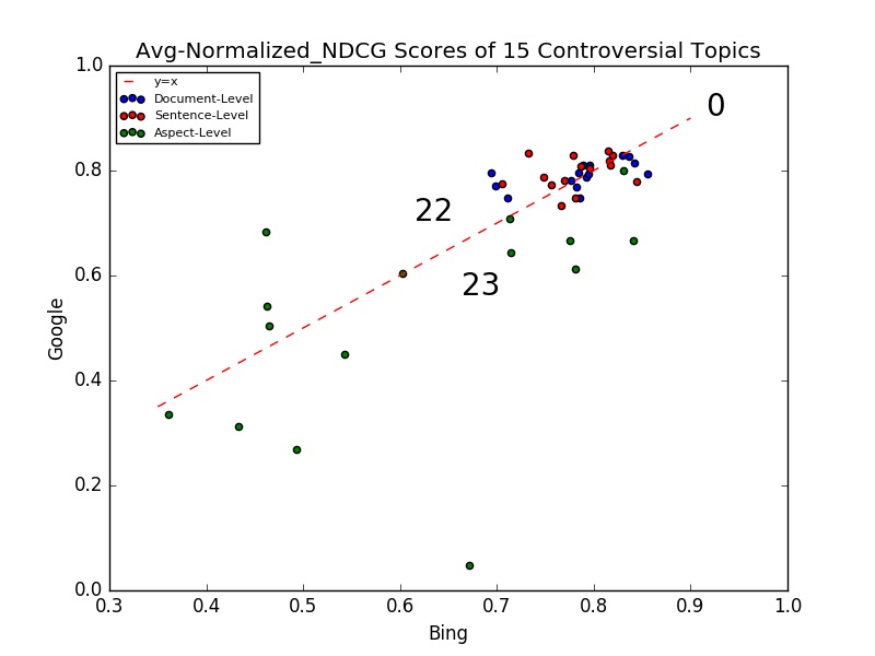
Figure 2. Avg-Normalized NDCG Scores of 15 Controversial Topics

In addition to the comparative analysis in terms of average NDCG-Senti scores for 15 controversial topics, we also compared two search engines by using NDCG-Senti scores of each query in a controversial topic. In this analysis, we compared two search engines per controversial topic and put the number of instances above/below and on the y=x axis to show the tendencies properly. While the previous analyses give the overall orientation of Bing & Google on the whole dataset, per-controversial topic plots can elaborately depict the differences in their attitudes towards the given topics. You can find sample results per each controversial topic below.

3.2.3. Statistical Significance Test

After having computed and plotted sentiment and NDCG-Senti scores in Figure 1 and 2 to understand the overall tendencies of two search engines, we also need to have a significance test to check if these differences are statistically significant. For this, we applied the following procedure:

• For each given data sample, check that it is normally distributed by creating a histogram from the data points.

  • If so, then go to next step.

  • If not, transform the data points by using ”log”, ”exp” etc.

    • Check that if the given data sample is normally distributed by creating a histogram from the transformed data points.

    • If not, try with a different transformation function for normality check and use other normality check methods such as QQplot until you observe that the data is normally distributed.

• Making sure that both of the data samples (Bing & Google) are normally distributed, apply F-test to see that the two data distributions have equal or unequal variances.

• Apply two-tail t-test with equal or unequal variances to understand if the means of these two distributions are significantly different.

You can find the two-tail p values with .95 confidence level in Table 6.

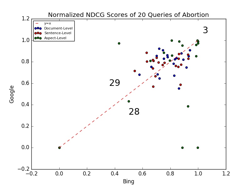
Figure 3. Normalized NDCG Scores of Abortion

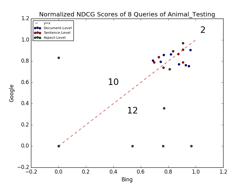
Figure 4. Normalized NDCG Scores of Animal Testing

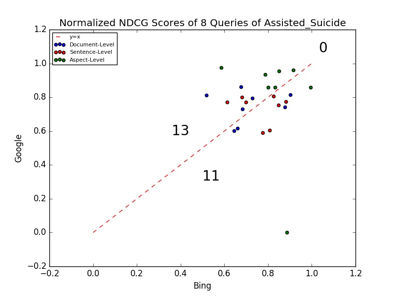
Figure 5. Normalized NDCG Scores of Assisted Suicide

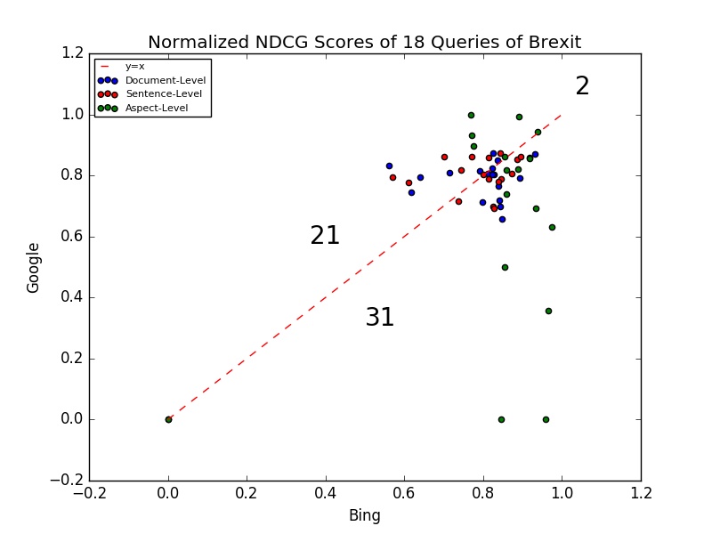
Figure 6. Normalized NDCG Scores of Brexit

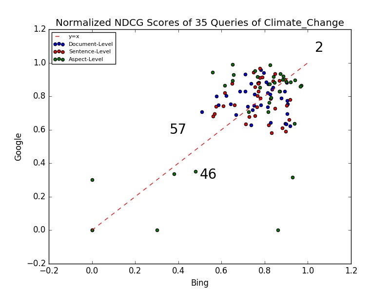
Figure 7. Normalized NDCG Scores of Climate Change

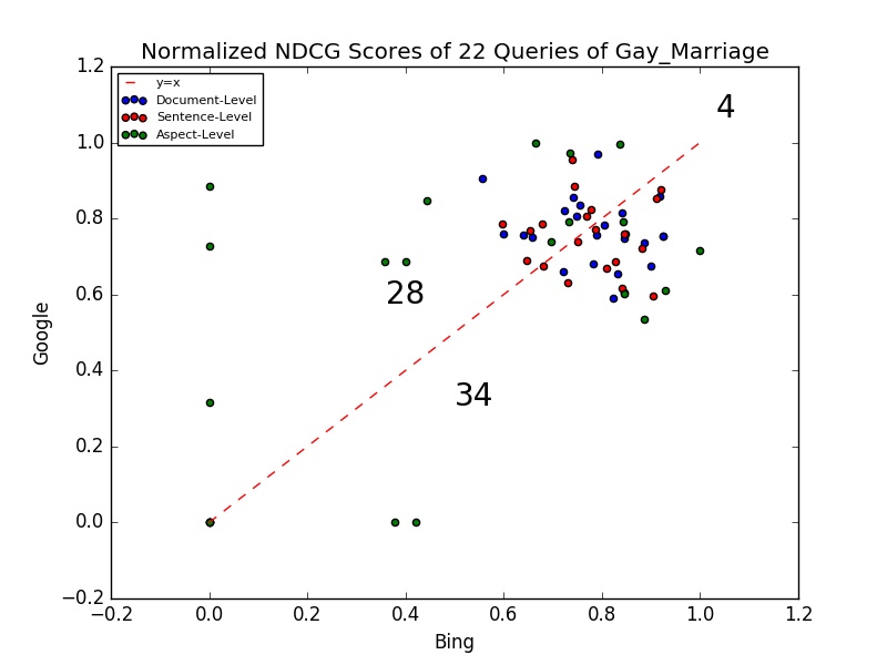
Figure 8. Normalized NDCG Scores of Gay Marriage

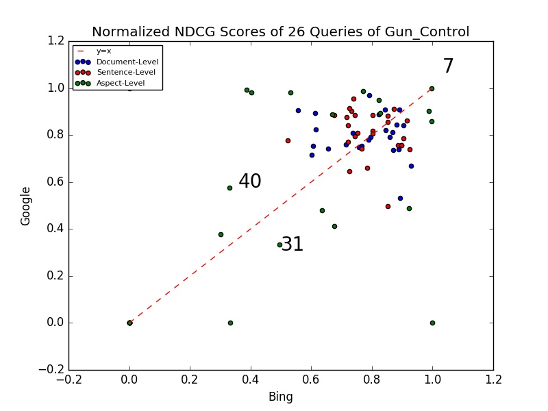
Figure 9. Normalized NDCG Scores of Gun Control

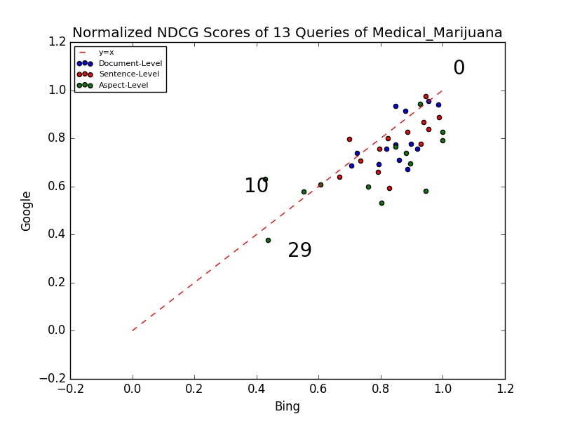
Figure 10. Normalized NDCG Scores of Medical Marijuana

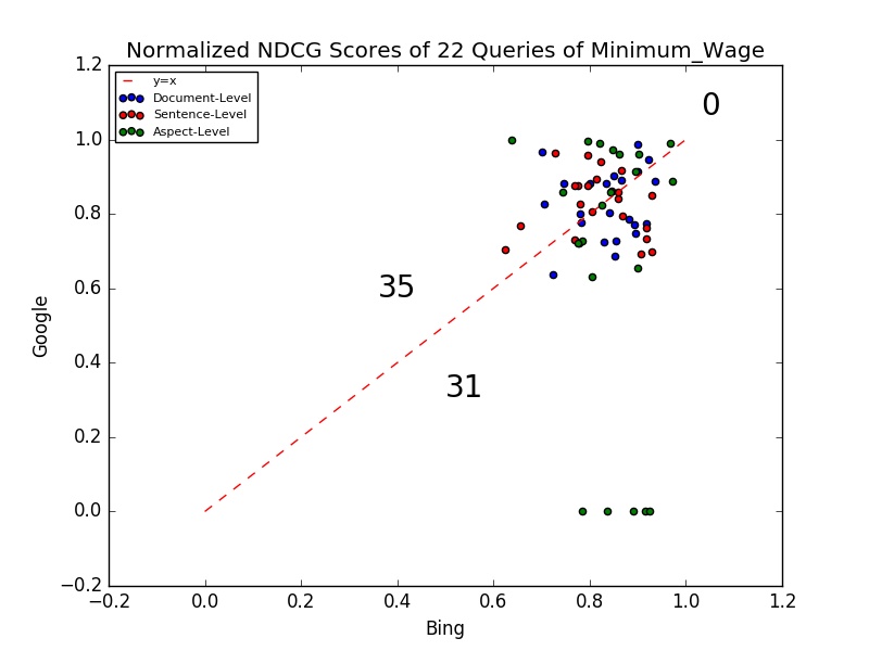
Figure 11. Normalized NDCG Scores of Minimum Wage

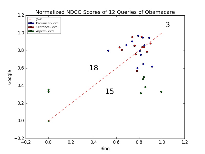
Figure 12. Normalized NDCG Scores of Obamacare

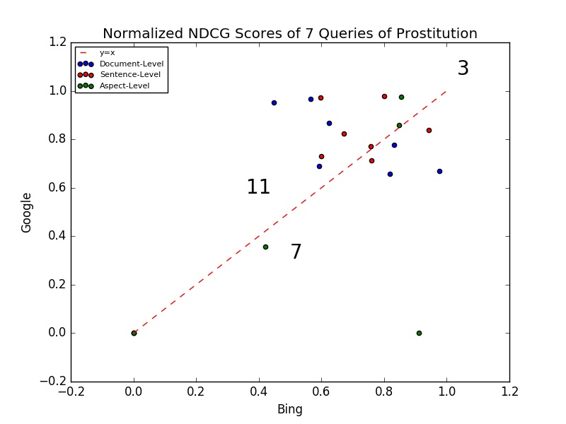
Figure 13. Normalized NDCG Scores of Prostitution

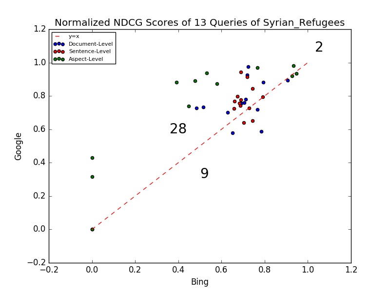
Figure 14. Normalized NDCG Scores of Syrian Refugees

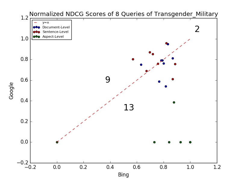
Figure 15. Normalized NDCG Scores of Transgender Military

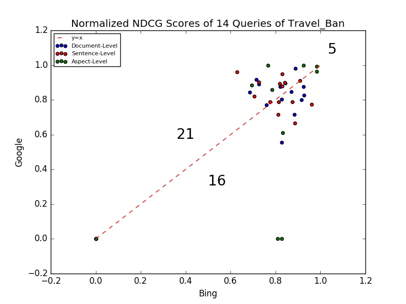
Figure 16. Normalized NDCG Scores of Travel Ban

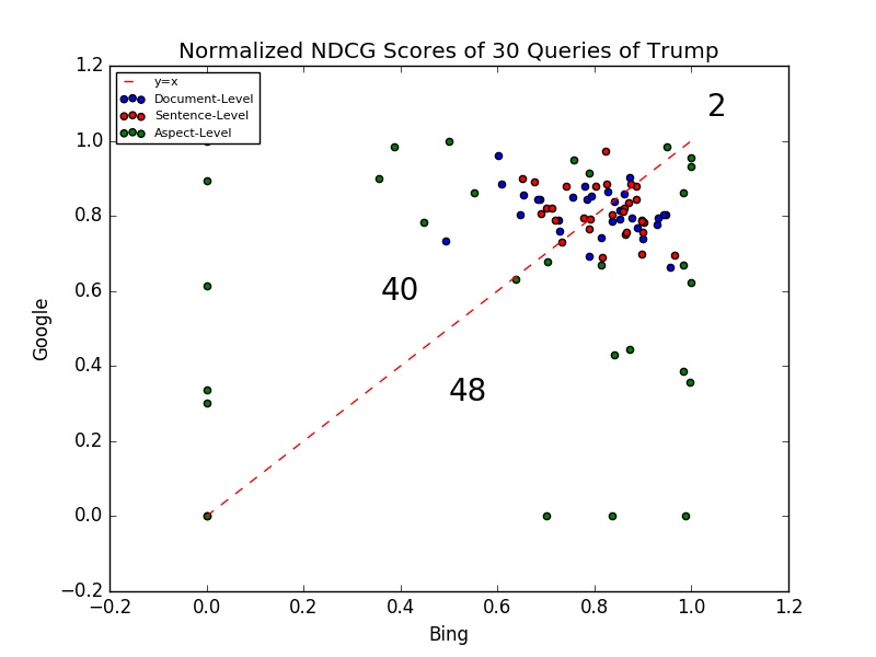
Figure 17. Normalized NDCG Scores of Trump

4. Future Work

For the effective crowd labelling framework, we are waiting for the acceptance. If the paper is accepted, then we will extend the existing framework. For the second part, we are preparing the results for conference publication. Afterwards, that part can be hopefully extended for journal publication.

References

- (1)
- Baccianella et al. (2010) Stefano Baccianella, Andrea Esuli, and Fabrizio Sebastiani. 2010. Sentiwordnet 3.0: an enhanced lexical resource for sentiment analysis and opinion mining.. In LREC, Vol. 10. 2200–2204.
- Manning et al. (2014) Christopher D. Manning, Mihai Surdeanu, John Bauer, Jenny Finkel, Steven J. Bethard, and David McClosky. 2014. The Stanford CoreNLP Natural Language Processing Toolkit. In Association for Computational Linguistics (ACL) System Demonstrations. 55–60. http://www.aclweb.org/anthology/P/P14/P14-5010