A Mathematical Programming Approach to Optimal Classification Forests

Abstract.

In this paper, we introduce Optimal Classification Forests, a new family of classifiers that takes advantage of an optimal ensemble of decision trees to derive accurate and interpretable classifiers. We propose a novel mathematical optimization-based methodology in which a given number of trees are simultaneously constructed, each of them providing a predicted class for the observations in the feature space. The classification rule is derived by assigning to each observation its most frequently predicted class among the trees in the forest. We provide a mixed integer linear programming formulation for the problem. We report the results of our computational experiments, from which we conclude that our proposed method has equal or superior performance compared with state-of-the-art tree-based classification methods. More importantly, it achieves high prediction accuracy with, for example, orders of magnitude fewer trees than random forests. We also present three real-world case studies showing that our methodology has very interesting implications in terms of interpretability.

1. Introduction

When it comes to creating a machine learning model, two fundamental factors are considered. On the one hand, the aim is to create models capable of making accurate predictions. On the other hand, we seek interpretability, since interpretable classifiers are preferable to black-box models (see e.g., Rudin et. al (2022)). Both features are known to be compatible although there often exists a trade-off between them. Accurate models tend to be more complex, and therefore difficult to interpret, whereas interpretable ones are usually less accurate. This is the case, for example, with Classification Trees (CTs) and Random Forests (RFs).

CTs are a family of classification methods built on a hierarchical relation among a set of nodes. A tree involves a set of branches connecting the nodes and defining the paths that observations can take by following a tree-shaped scheme. At the first stage of a CT method, all the observations belong to one node, which is known as the root node. From this node, branches are sequentially created by splits on the feature space, creating intermediate nodes (branch nodes) until the terminal nodes (leaf nodes) are reached. The predicted label for an observation is given by the most frequent class of the leaf node where it is located.

In contrast to the interpretable CT, Breiman (2001) introduced RF a method that creates an ensemble of trees (also called a forest) in order to combine their predictions so as to make a final prediction by means of voting. In RF, the number of trees involved in the ensemble is fixed, and usually large, which makes the model less interpretable. Each tree in the forest is constructed by drawing a random sample from the original training dataset and applying an algorithm to construct a classification tree. In general, RFs are more accurate models than a single decision tree, as well as more stable in terms of the selected points involved in the training dataset (Breiman, 2001; Bertsimas et. al, 2022).

CTs were initially presented from an algorithmic point of view, normally attending to greedy heuristic principles (Breiman et. al, 1984). However, whereas Optimal Classification Trees (OCTs) have been widely studied in the literature and have proven to provide numerous advantages (see e.g., (Carrizosa et. al, 2021)), to the best of our knowledge, the question of finding an optimal forest has not been previously studied.

In this paper, we take a first step in this direction and introduce the concept of an Optimal Classification Forest (OCF). We provide a mixed integer linear programming (MILP) formulation for the binary classification version of the problem. We show in our computational experiments that compared with a deep tree, an OCF can improve accuracy in small datasets with just a small number of shallow trees. This indicates that OCFs can potentially provide Pareto improvements over current methods, on both accuracy and interpretability. Moreover, we illustrate by means of some real examples how the solutions obtained are not only easier to interpret than those obtained with a CT, but also more flexible when being used. This is due to the fact that the first splits made in a deep CT have a strong impact on the following splits to be applied, whereas in an OCF this effect is mitigated due to the independence of the splits distributed among the different trees.

1.1. Literature

There are many different heuristic approaches to building a CT. The most popular method is CART, introduced by Breiman et. al (1984). CART is a greedy heuristic approach that myopically constructs a binary CT without anticipating future splits. Starting at the root node, it constructs the splits by means of separating hyperplanes minimizing an impurity measure at each of the branch nodes. Each split results in two new nodes and this procedure is repeated until a stopping criterion is reached. The trees derived from CART follow a top-down greedy approach, a strategy that is also shared by many other popular methods like C4.5 (Quinlan, 1993) or ID3 (Quinlan, 1996). One of the advantages of these top-down approaches is that the trees can be obtained rapidly even for large datasets, as the whole process is based on solving manageable problems at each node. Nevertheless, the optimality of these trees is not guaranteed because at each node the best split is sought without taking into account the splits to be made in deeper nodes. According to this, the obtained tree structures may not capture the correct distribution of the data, which may result in out-of-sample errors when making predictions. Moreover, these methods can generate very deep (complex) trees if high training set accuracy is desired, and this results in a direct loss of interpretability as well as an increased risk of overfitting. This problem is usually overcome by applying a post-process pruning of the trees, which generally consists of analyzing if it is worth splitting a given node by its improvement in the local classification rate.

On the other hand, Bertsimas and Dunn (2017) recently proposed an optimization approach to build a CT. This approach has been shown to outperform heuristic approaches. Optimal Classification Trees (OCTs) are capable of capturing hidden splits that may not have a strong local impact on the training task but allow the final model to be more accurate. OCTs have been a major field of study in recent years due to their good performance, and several algorithms have been designed to efficiently train them. Demirović et. al (2022), Lin et. al (2020) and Hu et. al (2019) propose different dynamic programming based algorithms to construct OCTs. Constraint Programming and SAT have also contributed to the OCT field with works such as those of Verhaeghe et. al (2020), Yu et. al (2020), Hu et. al (2020) or Narodytska et. al (2018). Moreover, we can see in Verwer and Zhang (2019) an alternative integer programming formulation to construct OCTs with a smaller number of decision variables than the one introduced by Bertsimas and Dunn (2017), as well as a column generation solution approach by Firat et. al (2020).

In order to obtain easily interpretable CTs, these are usually derived in their univariate version, i.e., with splits in which only one predictive variable is involved. Nevertheless, oblique CTs, trees where multiple predictive variables can be involved in the splits, have also been widely studied and one can find numerous heuristic methods in the literature,(Murthy et. al, 1994; Carreira-Perpiñán and Tavallali, 2018), as well as the oblique version of OCT, (OCT-H), introduced in Bertsimas and Dunn (2017), or other optimal methods as the one presented in Blanco et. al (2021).

As for the field of RF, since its introduction by Breiman (2001), it has become one of the most popular Machine Learning ensemble models, and some others such as gradient-boosted decision tree methods have been inspired by it. RF is a method that combines bagging (Breiman, 1996) and CART strategies, where different training sub-samples are obtained to grow a CT so that one can combine their predictions by means of a voting strategy. Its popularity is due to the fact that it has great advantages in terms of accuracy and training stability with respect to CTs, it does not have a large number of hyperparameters to calibrate (as initially only one is added, the number of trees, with respect to those involved in CART), and it can be easily adapted to parallel computational strategies due to its own nature. Therefore, improvements in this method with different ways of obtaining the training samples and ways to randomize the trees have been studied in the literature (see Biau and Scornet, 2016). Furthermore, an implementation of boosted trees, derived from a trees ensemble, XGBoost, has become one of the most popular machine learning methods as we can see reflected, for instance, in the fact that it was used in most of the winning ideas in Kaggle data science competitions in 2015 (Chen and Guestrin, 2016). However, despite its many advantages, the major drawback of the method is the loss of interpretability as the number of trees in the ensemble increases.

In recent years, mathematical optimization has brought great advances in Machine Learning. As well as in tree-shaped classification rules, in methods such as Support Vector Machines (SVM), mathematical optimization plays a crucial role as the classifiers are derived directly from the solution of an optimization problem (Cortes and Vapnik, 1995; Blanco et. al, 2020a, b). Furthermore, by means of properly modifying the objective function and constraints of a given optimization problem, one can adapt the methods to scenarios such as variable selection (Günlük et. al, 2021; Baldomero-Naranjo et. al, 2020, 2021), problems with special accuracy requirements (Benítez-Peña et. al, 2019; Gan et. al, 2021), or problems with unbalanced and noisy instances (Eitrich and Lang, 2006; Blanco et. al, 2022; Blanquero et. al, 2021). For this reason, numerous studies combining machine learning and mathematical optimization continue to be carried out and are a field of great interest because of their successes in practical applications.

Nevertheless, as far as we know, there is not much work in the literature on the use of mathematical optimization to derive tree ensembles. In Mišić (2020), the authors consider a given tree ensemble that predicts a target continuous variable using controllable independent variables (given a certain application), and they study how to set these independent variables in order to maximize the predicted value by means of a MILP. Apart from this, we could not find in the literature anything regarding optimal tree ensembles for classification problems.

1.2. Contributions and Structure

This paper introduces the concept of the Optimal Classification Forest (OCF). For this purpose, we derive a MILP formulation to classify binary class instances. The main advantage of OCFs as opposed to existing RF is to drastically reduce the number of trees involved in the ensemble, resulting in more interpretable classification rules without significant loss of accuracy. Across 10 real data sets, we show a fair comparison in terms of accuracy using OCFs, CART, OCTs and RFs, showing that OCF results match or outperform other existing CT-based methods and obtain comparable results with respect to RFs. Furthermore, we analyze in detail three real-world case studies where we further analyze the solutions obtained by OCFs, concluding that our tool provides classifications rules which are easy to interpret and flexible to apply, as opposed to more rigid and complex solutions provided by complex CTs.

In Section 2 we introduce the problem under study and fix the notation used throughout the paper. Section 3 presents the mathematical programming formulation of the binary OCF. In Section 4 we present the results of our computational experiments comparing OCFs with RFs and CT-based methodologies. In Section 5 we analyze in detail the solutions provided by OCFs and OCTs over three real case studies. Finally, in Section 6 we report our conclusions.

2. Preliminaries

In this section, we introduce the concept of OCF and recall the main elements that set the base for the approach that is presented in Section 3, i.e. the main concepts regarding CTs.

All throughout this paper, we consider that we are given a training sample $\mathcal{X}=\{(x_{1},y_{1}),\ldots,(x_{n},y_{n})\}\subseteq\mathbb{R}^{p}\times\left\{0,1\right\}$, where $p$ features have been measured for a set of $n$ individuals ($x_{1},\ldots,x_{n}$) as well as a label in $\{0,1\}$ for each of them $(y_{1},\ldots,y_{n})$. The goal of binary supervised classification is to derive, from $\mathcal{X}$, a decision rule $D_{\mathcal{X}}:\mathbb{R}^{p}\rightarrow\{0,1\}$ capable of accurately predicting the label of out-of-sample observations. We assume, without loss of generality, that the features are normalized, i.e., $x_{1},\ldots,x_{n}\in[0,1]^{p}$, and we denote by $N=\{1,\ldots,n\}$ the index set for the observations in the training dataset.

As already pointed out, CTs are classifiers based on a hierarchical relationship among a set of nodes. The decision rule for a CT method is built by recursively partitioning the feature space by means of hyperplanes. In the first stage, a root node for the tree is considered which all the observations belong to. Branches are sequentially created, at the so-called branch nodes, by splits on the feature space, creating intermediate branch nodes until a leaf node, nodes where no more splits are made, is reached. Specifically, at each branch node, $t$, of the tree a hyperplane $\mathcal{H}_{t}=\{z\in\left[0,1\right]^{p}:{(a_{t})}^{\intercal}z=b_{t}\}$ is constructed (note that ${(a_{t})}^{\intercal}$ stands for the transpose operator applied to the vector $a_{t}\in\left[0,1\right]^{p}$) and the splits are defined as ${(a_{t})}^{\intercal}z<b_{t}$ (left branch) and ${(a_{t})}^{\intercal}z\geq b_{t}$ (right branch). In a CT, we call depth the maximum number of splits that can be made before reaching a leaf node. Given a maximum depth, $D$, a CT can have at most $T=2^{D+1}-1$ nodes. These nodes are differentiated into two types:

• Branch nodes: $\tau_{B}=\left\{1,\ldots,\lfloor T/2\rfloor\right\}$ are the nodes where splits can be applied.

• Leaf nodes: $\tau_{L}=\left\{\lceil T/2\rceil,\ldots,T\right\}$ are the nodes where predictions for observations are performed.

On the other hand, according to the notation used to describe the hierarchical relationships in the tree, we define $p(t)$ as the parent of node $t$, for $t=2,\ldots,T$. We define $A_{L}(t)$ (resp $A_{R}(t)$) as the set of left (resp. right) ancestors of node $t\in\{2,\ldots,T\}$, which are the nodes whose left (resp right) branch has been followed on the path from the root node to $t$.

As an example, in Figure 1 we show a simple OCT with depth two, for a small dataset with $13$ observations. This CT has three branch nodes and four leaf nodes. Besides, it only has one misclassification error, since one blue point is lying in a leaf node where the red class (the most represented class in the leaf) is assigned.

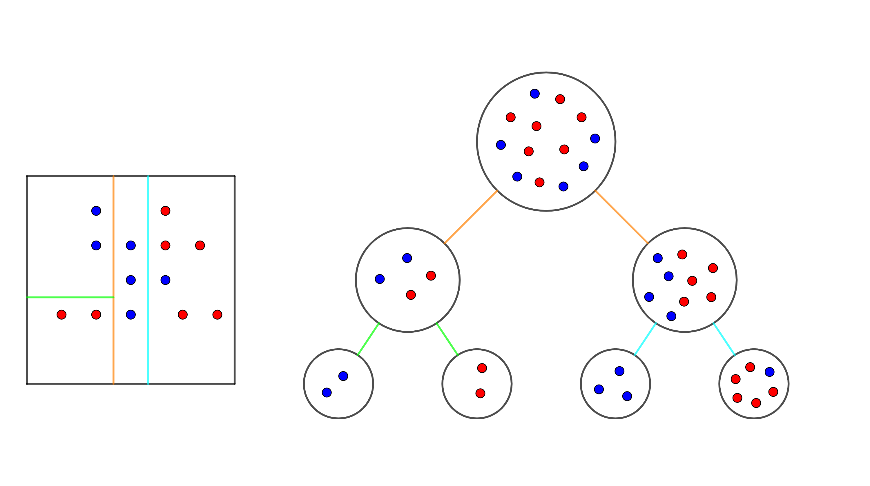
Figure 1. Binary classification problem with its split solution in $\left[0,1\right]^{2}$ (left) and its OCT graph-solution form (right)

According to this example, to achieve a perfect classification rate, in the context of the OCTs we would have to follow a vertical approach, i.e. increase the OCT depth. In contrast, we propose a horizontal approach through an OCF to achieve the same end. In this respect, we define an $R$-OCF (for $R\in\mathbb{Z}_{+}$) as a set of $R$ CTs that combine their predictions using a majority voting strategy in the leaves to construct a global prediction. In this ensemble, all trees have access to the entire training sample and knowledge of what errors are occurring in the other trees in order to coordinate with each other and optimize their strategy. Note that with this definition, the CTs that form an OCF do not necessarily have to be optimal (in the sense of OCT) for a given depth, and furthermore, neither they have to follow a fixed pattern when it comes to generating splits as in the case of heuristic algorithms, they have to be adequately coordinated to obtain a good final accuracy when voting. To illustrate this paradigm, we show in Figure 2 a solution of the previous example with an OCF consisting of $3$ CTs of depth $2$.

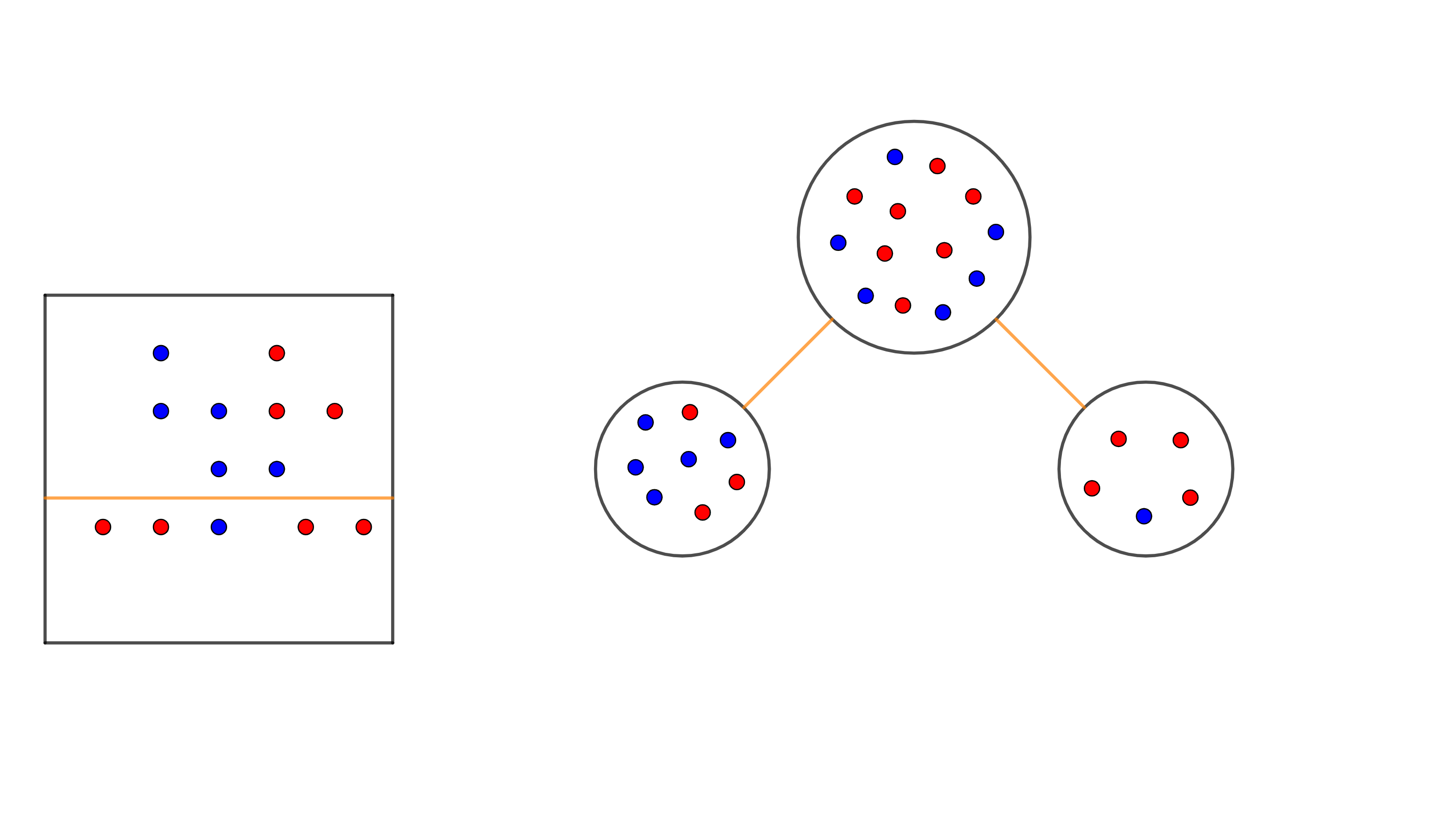
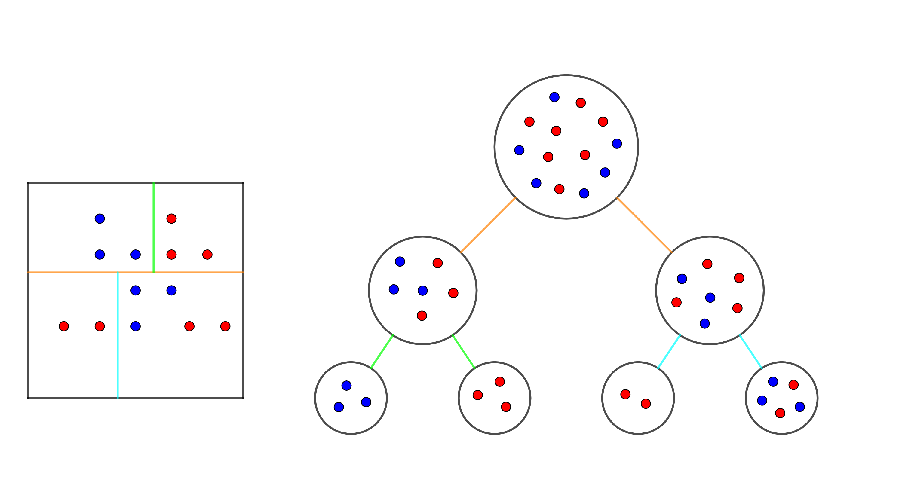
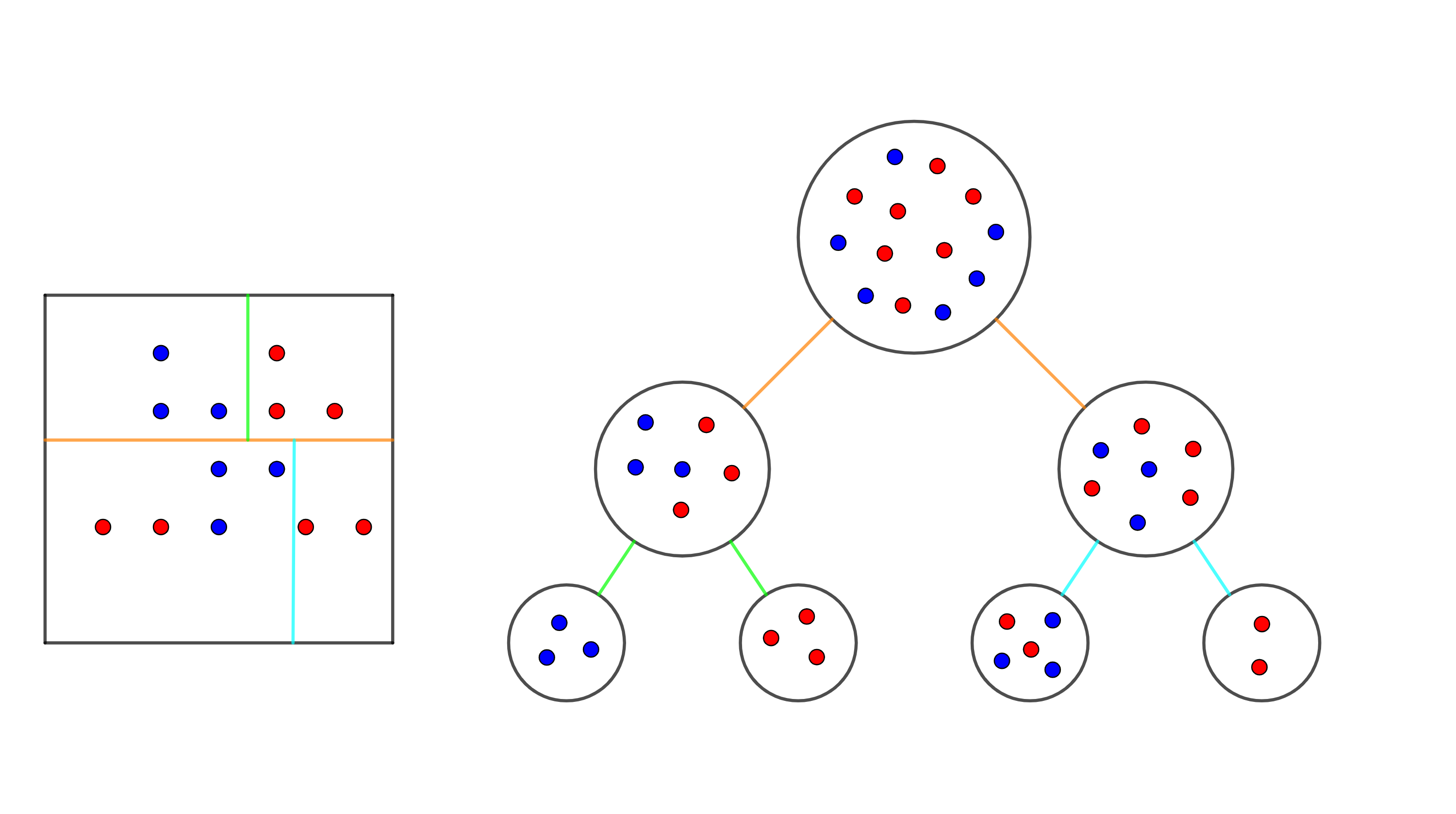
Figure 2. Optimal classification forest solution.

Looking at each of the trees individually, all of them have non-zero misclassification errors. In Figure 3 we can see the misclassified observations in each tree coloured in black.

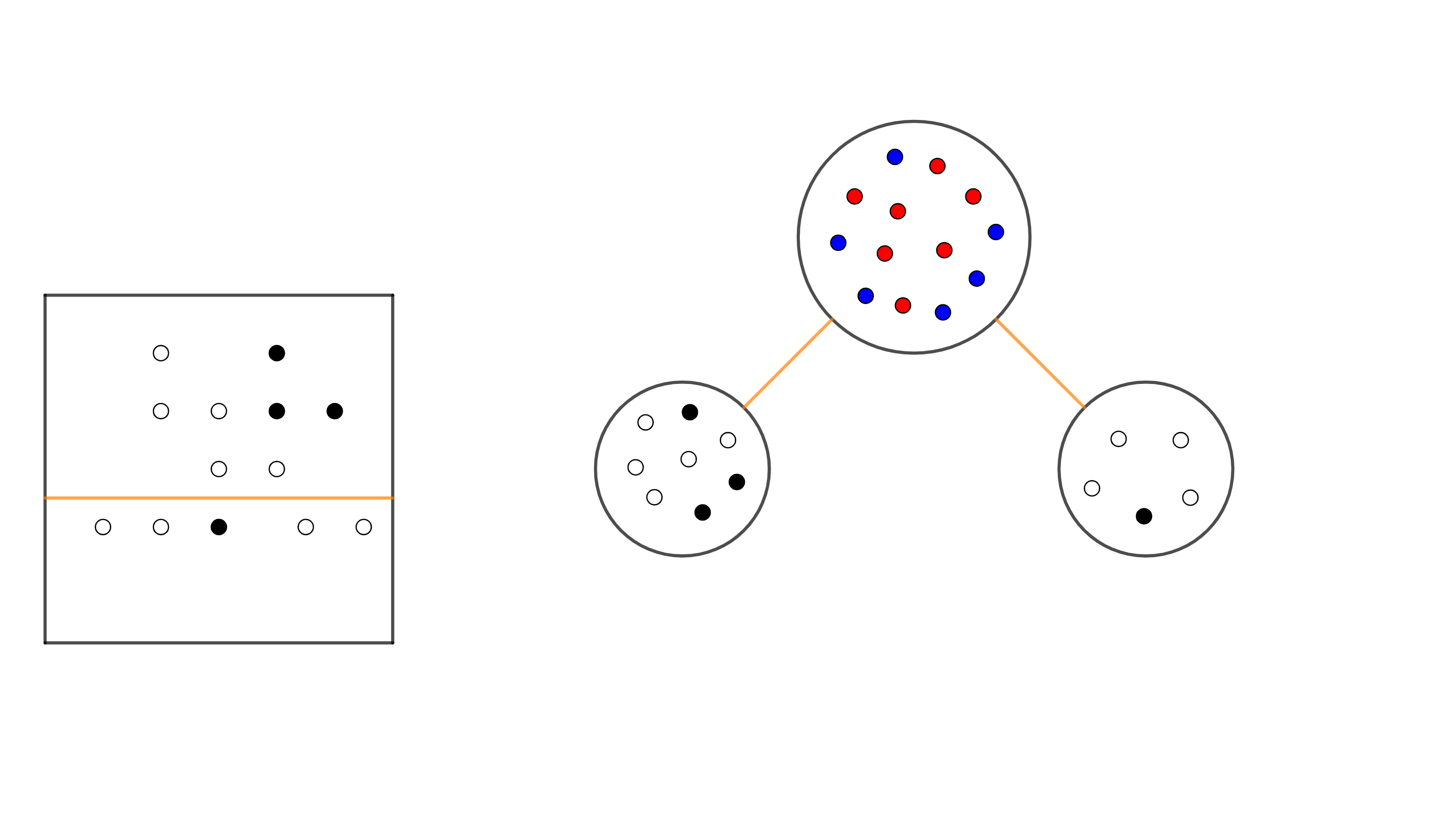
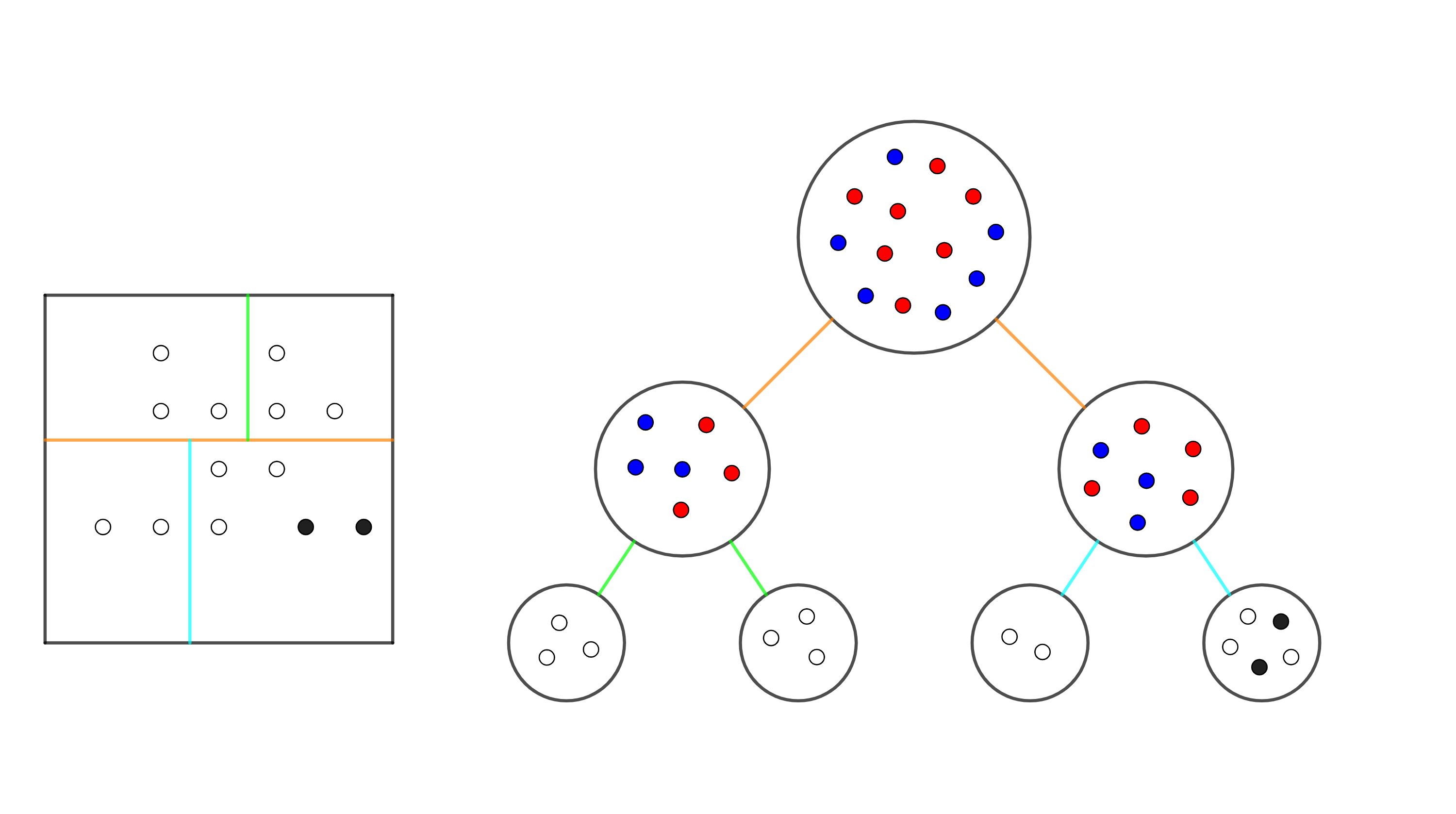
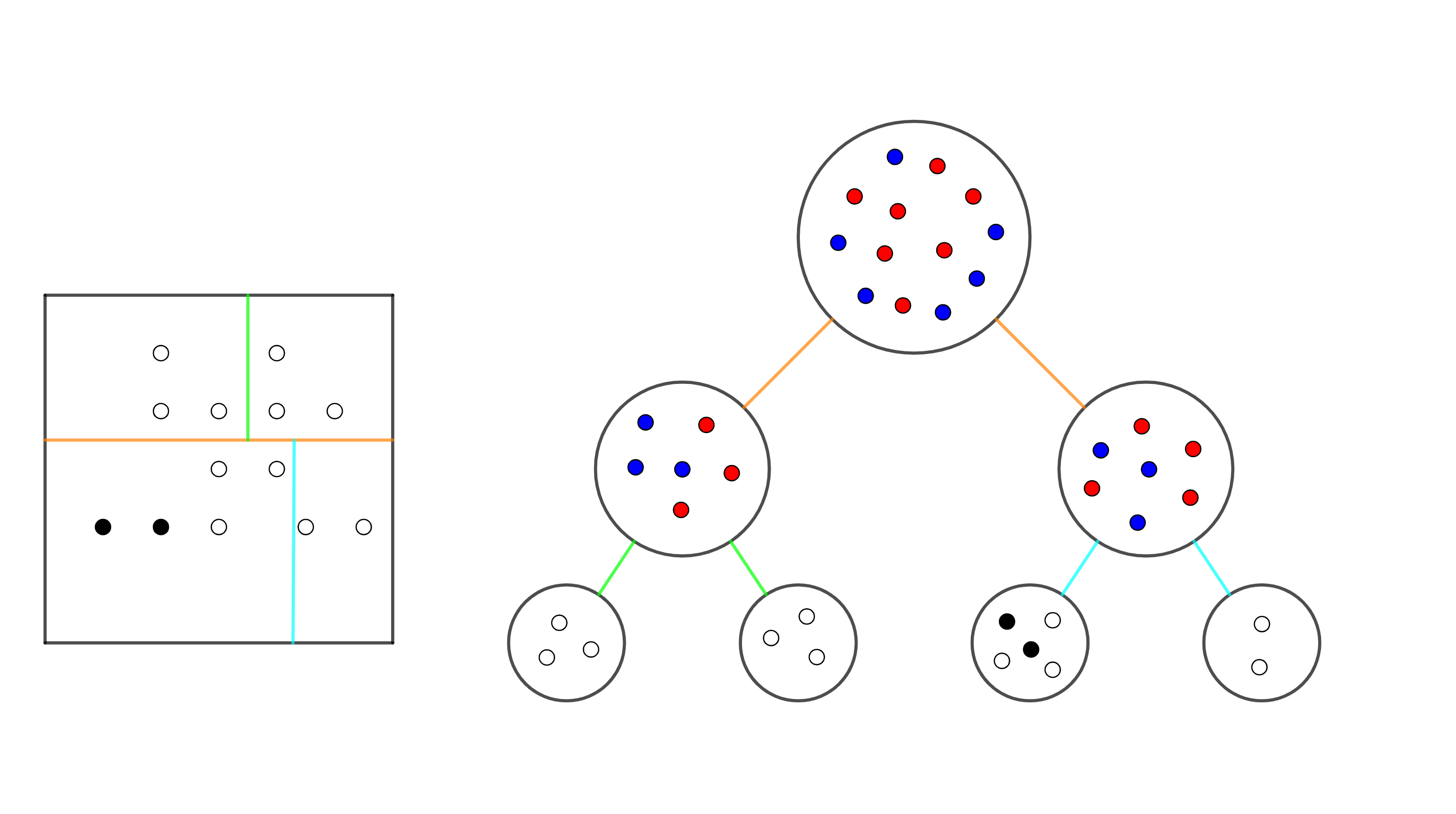
Figure 3. Misclassifications occur in individual trees.

Nevertheless, we can see that none of the observations are coloured in more than one tree, and therefore, if we were to follow a voting classification strategy, every observation would have at least two votes associated with its correct class and consequently no observation would be finally misclassified.

At this point, one can observe that given a training sample, one can always calibrate the hyperparameters of OCTs and OCFs to increase their training accuracy. In OCTs, increasing the depth has a direct impact on the training accuracy. In OCFs, both the depth of the trees and the number of them allow us to increase such accuracy. Splits created in a deep OCT, however, decrease its “marginal efficiency”, because later splits are conditioned on the previous ones. In other words, deep splits could affect only small subsamples of the training sample, and this could lead to overfitting. On the other hand, the splits in OCF have less dependency and are more efficient. Thus even if OCT and OCF have comparable training accuracy, OCF might achieve better out-of-sample performance. This is indeed the case in the computational experiments we performed, as shown in Section 4.

3. Mathematical Programming Formulation

This section is devoted to providing a mathematical programming formulation of the OCF for binary instances derived by a forest $\mathcal{F}$ with a fixed odd number of trees, $R$. In order to do this, we start by presenting the objective function of the problem. As it is done in OCT, we minimize the misclassification errors within the training sample as well as the complexity of the ensemble, which is the number of active splits involved in all the trees. Recalling that $y_{i}\in\{0,1\},\forall i=1,\ldots,n,$ we define a binary variable $\alpha_{i}$ for each observation $i=1,\ldots,n,$ that takes value one in case the ensemble predicts class $1$ for observation $i$, and zero otherwise. Moreover, we use the binary variables $d^{r}_{t}\in\{0,1\}$ to model if tree $r$ splits at node $t$. According to these, the objective function of our problem is given by the following expression:

$\displaystyle\min\frac{1}{n}\sum_{i=1}^{n}\lvert y_{i}-\alpha_{i}\rvert+C\sum_{r=1}^{R}\sum_{t\in\tau_{b}}d_{t}^{r}$.

That is, the sum of the number of observations that are incorrectly classified (according to the $\alpha$-variables) plus the number of splits in the ensemble. Trees minimizing the above expressions will be constructed.

In what follows we detail the constraints relating to the different variables in our model and that must also ensure that a forest is adequately constructed.

First, we need to ensure that the $\alpha$-variables are properly defined, representing the final result of the voting strategy amongst the $R$ trees. With this goal in mind, we define the binary variables $\theta^{r}_{i},\forall i=1,\ldots,n,r=1,\ldots,R,$ which take the value one if class one is predicted in tree $r$ to observation $i$, and takes value zero otherwise, and we add the following constraints to the problem:

$$\sum_{r=1}^{R}\frac{\theta_{i}^{r}}{R}-\frac{1}{2}\leq\alpha_{i}, \forall i=1,\ldots,n,$$ (1)

$$-\sum_{r=1}^{R}\frac{\theta_{i}^{r}}{R}+\frac{1}{2}\leq 1-\alpha_{i}, \forall i=1,\ldots,n.$$ (2)

Note that in case more than half of the trees vote class one for observation $i$, constraint (1) will be activated and force the $\alpha_{i}$ to take the value one. On the other hand, in case that less than half of the trees vote class one for observation $i$, constraint (1) will not be activated but constraint (2) will, forcing the $\alpha_{i}$ to take the value zero. Since the number of trees is an odd number, ties will not occur.

With the above constraints and our objective function, we assure that the voting strategy is well modeled. In this regard, once the basis of the problem has been established, we require each of the trees to be adequately defined. To this end, we also consider the following set of decision variables to regulate the rationale of the splits in the tree as well as the allocation of the observations to the leaves:

• $z^{r}_{it}=\left\{\begin{array}[]{cl}1,&\mbox{if observation $i$ belongs to node $t$ in tree $r$,}\\ 0,&\mbox{otherwise,}\end{array}\right.$ for all $i\in N$, $t\in\tau_{l}$, $r\in\mathcal{F}$.

• $d^{r}_{t}=\left\{\begin{array}[]{cl}1,&\mbox{if a split is applied at node $t$ in tree $r$,}\\ 0,&\mbox{otherwise,}\end{array}\right.$ for all $t\in\tau_{b}$, $r\in\mathcal{F}$.

• $l^{r}_{t}=\left\{\begin{array}[]{cl}1,&\mbox{if $t$ is a non-empty leaf in tree $r$,}\\ 0,&\mbox{otherwise,}\end{array}\right.$ for all $t\in\tau_{l}$, $r\in\mathcal{F}$.

• $a^{r}_{t}\in\{0,1\}^{p},b^{r}_{t}\in[0,1]$: coefficients and the intercept of the split involved at node $t$ in tree $r$, for all $t\in\tau_{b}$, $r\in\mathcal{F}$.

In contrast to other CTs methodologies OR do to track the number of misclassification errors occurred in the leaf nodes of the trees. However, we have to make sure that if two observations belong to the same leaf node in a certain tree, they must be assigned to the same class in such a tree. In order to do this, we incorporate to our formulation the following constraints:

$$2-z_{it}^{r}-z_{jt}^{r}\geq\lvert\theta_{i}^{r}-\theta_{j}^{r}\rvert, \forall i,j\in N(i<j),r\in\mathcal{F},\ t\in\tau_{l}.$$ (3)

Note that if two observations $x_{i}$ and $x_{j}$ belong to leaf node $t$ in tree $r$, then $z_{it}^{r}+z_{jt}^{r}=2$, and thus $\theta_{i}^{r}=\theta_{j}^{r}$. According to this, since this constraint affects to all observations that belong to leaf $t$ in tree $r$, we assure that one, and only one, class is assigned to each leaf node $t$ in tree $r$.

In the following, each of the trees in the ensemble should be adequately defined. We model this structure analogously to other OCT models. For all $r\in\mathcal{F}$:

$$\sum_{q=1}^{p}a_{tq}^{r}=d_{t}^{r},\forall t\in\tau_{b},, 4^{r}$$ ()

$$0\leq b_{t}^{r}\leq d_{t}^{r},\forall t\in\tau_{b}, 5^{r}$$ ()

$$d_{t}^{r}\leq d_{p(t)}^{r},\forall\in\tau_{b}\backslash\{1\}, 6^{r}$$ ()

$$\sum_{t\in\tau_{l}}z_{it}^{r}=1,\forall i\in N, 7^{r}$$ ()

$$z_{it}^{r}\leq l_{t}^{r},\forall i\in N,\ t\in\tau_{l},\ 8^{r}$$ ()

$$\sum_{i=1}^{n}z_{it}^{r}\geq n_{\text{min}}l_{t}^{r},\forall t\in\tau_{l}, 9^{r}$$ ()

$$(a_{m}^{r})^{\intercal}x_{i}+\epsilon\leq b_{m}^{r}+(1+\epsilon)(1-z_{it}^{r}),\forall i\in N,\ t\in\tau_{l}, 10^{r}$$ ()

$$m\in A_{L}(t),$$

$$(a_{m}^{r})^{\intercal}x_{i}\geq b_{m}^{r}-(1-z_{it}^{r}),\forall i\in N,\ t\in\tau_{l}, 11^{r}$$ ()

$$\ m\in A_{R}(t).$$

According to this, Constraints ($4^{r}$) and ($5^{r}$) enforce that the (univariate) splits are only applied in active nodes $(d^{r}_{t}=1)$. Note that oblique splits could be similarly applied by slightly modifying these constraints. Nevertheless, we maintain orthogonal splits so as to retain the interpretability of the final model. The hierarchical structure of a tree is given in constraint ($6^{r}$). Note that if the parent node of node $t$ does not create a split, then node $t$ should not create a split itself, i.e., $d^{r}_{p(t)}=0$ implies $d^{r}_{t}=0$. In case $t$ creates a split, then its parent node must also create a split, so $d^{r}_{t}=1$ implies $d^{r}_{p(t)}=1$. Constraint ($7^{r}$) ensures that an observation belongs to exactly one leaf node for each tree. Constraints ($8^{r}$) and ($9^{r}$) imply that a leaf node is non-empty if and only if there are at least $n_{\text{min}}$ observations in the leaf node. Constraints ($10^{r}$), where $\epsilon$ is a small positive constant, and ($11^{r}$) force observations belonging to leaf $t$ in tree $r$ to satisfy all the splits in order to reach the leaf node $t$ from the root node in tree $r$.

Gathering all together, the binary OCF can be formulated as the following MILP problem:

$$\min\;\; \;\;\frac{1}{n}\sum_{i=1}^{n}\lvert y_{i}-\alpha_{i}\rvert+C\sum_{r=1}^{R}\sum_{t\in\tau_{b}}d_{t}^{r} {\rm OCF\ }$$ ()

s.t. $$\ \eqref{OCF-1}-\eqref{OCF-3},$$

$$\eqref{OCF-4}-\eqref{OCF-11},\forall r\in\mathcal{F},$$

$$\alpha_{i}\in\left\{0,1\right\},\forall i\in N,$$

$$\theta_{i}^{r}\in\left\{0,1\right\},\forall i\in N,\ r\in\mathcal{F},$$

$$d_{t}^{r}\in\left\{0,1\right\},\ a_{t}^{r}\in\left\{0,1\right\}^{p},\ b_{t}^{r}\in\left[0,1\right],t\in\tau_{b},r\in\mathcal{F},$$

$$l_{t}^{r}\in\left\{0,1\right\},t\in\tau_{l},\ r\in\mathcal{F},$$

$$z_{it}^{r}\in\left\{0,1\right\},\forall i\in N,\ t\in\tau_{l},r\in\mathcal{F}.$$

4. Computational Experiments

In this section, we present the results of our computational experiments, with the aim of studying the predictive capacity of OCF with respect to other similar methods. Since the idea is to obtain interpretable classifiers, as we show in the next section, we study simple versions of the possible resulting models. Five methods are compared: CART, OCT, RF with 3 trees (3-RF), RF with 500 trees (500-RF), and OCF with three trees (3-OCF). All these methods have been applied to ten real-life datasets from the UCI Machine Learning Repository (Lichman, 2013). The datasets’ names and dimensions ($n$: number of observations, $p$: number of features) are reported in the first column of Table 1.

To establish a fair comparison over the datasets where all observations are involved at some point as a training, validation or test set, we perform a 4-fold cross-validation scheme, i.e., datasets are split into four random train-validation-test partitions. Two of the folds are used for training the model, one of them is used as a validation set for calibrating the parameters of the models, and the remaining one is used for testing. For each method, we choose the combination of parameters with a better performance (in terms of accuracy) in the validation sample and use that model to compute the accuracy, in percentage, for the test set. Finally, in order to avoid taking advantage of beneficial initial train-validation-test partitions, we repeat the cross-validation process 5 times and report the average accuracy and standard deviation.

With regard to the parameters involved in CART and OCT, we set the minimum amount of observations allowed to be in a leaf node, $n_{\text{min}}$, to be $2.5\%$ of the training sample size, and the depth of the trees, $D$, is set to three. Moreover, as it is done by Bertsimas and Dunn (2017), instead of calibrating a complexity parameter, we remove the complexity term from the objective function and add the following constraint that upper bounds the number of active splits:

$$\sum_{t\in\tau_{b}}d_{t}\leq C.$$

where $C\in\{1,\ldots,7\}$ is the parameter to be tuned during validation.

For the 3-OCF, we use a smaller depth, $D=2$, and set $n_{\text{min}}$ to be $2.5\%$ of the training sample. For a fair comparison, we limit the total number of splits to be smaller than seven and tune $C\in\{1,\ldots,7\}$ in the 3-OCF:

$$\sum_{r\in\mathcal{R}}\sum_{t\in\tau_{b}}d_{t}^{r}\leq C.$$

For the 3-RF and 500-RF, we also let the trees have a maximum depth equal to two, $D=2$, and each of the trees is built over a random sample of $n=75$ points with access to the whole set of predictor variables.

In addition to this downsampling technique, the OCF model is provided with a new symmetry-breaking constraint to help in its resolution. Note that the OCF model exhibits symmetry. Each feasible forest is equivalent (in objective value) to all permutations in the tree indices $r$. It is well-known that symmetric discrete optimization models may be computationally costly since deeper branch-and-bound trees are to be constructed to guarantee the optimality of the solutions. To avoid this symmetry, we incorporate into our model the following symmetry-breaking constraints:

$$\displaystyle\sum_{i=1}^{n}\left|\theta_{i}^{1}-\alpha_{i}\right|\leq\displaystyle\sum_{i=1}^{n}\left|\theta_{i}^{2}-\alpha_{i}\right|\leq\ldots\leq\displaystyle\sum_{i=1}^{n}\left|\theta_{i}^{R}-\alpha_{i}\right|.$$

These constraints sort the indices in the trees by a number of misclassified training observations.

Additionally, both OCT and OCF formulations have a family of constraints that involves a small enough parameter, which has been fixed to the value $\epsilon=0.00001$ in all the experiments. On the other hand, in terms of the number of binary variables involved in OCT and OCF, they increase exponentially with respect to the depth of a tree, and linearly with respect to the number of trees in an OCF. However, when considering a small depth and a small number of trees, OCF is more computationally challenging. Thus, we applied an additional downsampling technique in order to reduce the training data set from $50\%$ of the original data to a fixed number of $75$ points. We do this reduction by taking 5 random samples in each of the experiments. Therefore, we choose the combination of the training sample and complexity parameter that works best in the validation set and provide the result obtained with that model in the test. We also tried this technique with CART and OCT, but the results obtained were slightly inferior to the ones obtained when training with the whole training sample.

Finally, we warm-start the OCT by the most discriminatory split amongst the set of variables at the root node, and we give each tree in the optimal classification forest the most discriminatory split amongst one-third of the feature variables. The models were coded in Python and solved using the optimization solver Gurobi v9.5.1. In all cases, a time limit of one hour was set and most of the instances were not solved to optimality. The experiments were run on a PC Intel Xeon E-2146G processor at 3.50GHz and 64GB of RAM.

We show in Table 1 the results obtained in all the experiments. We report the average accuracy (and standard deviations) of the five methods for each of the five datasets. The most remarkable observation, in view of the results, is that 3-OCF outperforms the other classification tree methods in most of the datasets. Moreover, it achieves results comparable to those of 500-RF. In this sense, in these small datasets, we show a Pareto improvement in terms of accuracy versus interpretability. We obtain better results in accuracy compared to the interpretable models ($3$-RF and CTs) and better results in terms of interpretability compared with complex random forests, as 500-RF. In the Heart dataset, the improvement is even more impressive: $3$-OCF’s accuracy is more than $3\%$ higher with respect to $500$-RF, $6\%$ higher with respect to OCT, and $9\%$ higher with respect to CART.

	CART	OCT	3-RF	500-RF	3-OCF
Australian Credit (690, 14)	84.16 $\pm$ 1.71	84.36 $\pm$ 2.28	80.06 $\pm$ 4.83	85.12 $\pm$ 2.10	84.08 $\pm$ 2.22
Breast Cancer (683, 9)	92.14 $\pm$ 1.81	94.24 $\pm$ 1.89	94.28 $\pm$ 2.21	96.21 $\pm$ 1.50	94.24 $\pm$ 1.32
German Credit (1000, 24)	70.70 $\pm$ 3.14	71.42 $\pm$ 3.32	69.65 $\pm$ 3.79	72.07 $\pm$ 2.27	71.12 $\pm$ 2.91
Heart (Statlog) (270, 13)	74.36 $\pm$ 4.87	76.91 $\pm$ 4.49	74.45 $\pm$ 5.22	80.16 $\pm$ 4.94	83.19 $\pm$ 4.23
ILDP (552, 10)	67.19 $\pm$ 3.93	68.15 $\pm$ 2.80	67.31 $\pm$ 3.53	68.25 $\pm$ 3.59	71.11 $\pm$ 4.33
Ionosphere (351, 33)	88.11 $\pm$ 3.28	88.55 $\pm$ 3.66	88.52 $\pm$ 4.04	90.68 $\pm$ 3.83	89.63 $\pm$ 3.36
RA-Parkinson (240, 40)	72.13 $\pm$ 6.66	75.19 $\pm$ 5.97	75.94 $\pm$ 6.60	77.72 $\pm$5.09	77.37 $\pm$ 5.25
Sonar (208, 60)	65.02 $\pm$ 5.90	71.04 $\pm$ 7.06	69.10 $\pm$ 9.20	72.72 $\pm$ 6.39	70.77 $\pm$ 7.03
SPECT Heart (683, 9)	75.79 $\pm$ 5.38	76.69 $\pm$ 4.57	76.40 $\pm$ 6.19	78.27   $\pm$ 5.57	79.38 $\pm$ 5.87
Vertebral (310, 6)	79.75 $\pm$ 4.43	80.13 $\pm$ 4.35	81.15 $\pm$ 4.38	81.94 $\pm$ 4.42	81.41 $\pm$ 3.05

Table 1. Average accuracy $\pm$ std obtained in our computational experiments.

5. Case Studies

In the previous section we studied the predictive ability of our model with respect to its tree-shaped benchmarks. We showed how the model is able to broadly improve the accuracy of interpretable CT-based models, but we did not discuss in detail the obtained solutions. As we have pointed out throughout this paper, in the context of machine learning, solutions that are interpretable by humans are preferable to black-box approaches where it is not possible to identify why a certain class was predicted to a given observation.

In practice we often find that for certain datasets numerous classifiers report very similar accuracy results (this is indeed the case in some of our computational experiments), and in these cases there is no dispute that it is better to use the simpler models. On the other hand, the work presented by Rudin et. al (2022) points out that when several classifiers of different nature report the same accuracy, there should be a simple and interpretable model that preserves accuracy. However, finding such a simple model, in case of existence, can be very challenging.

In this section we present the analysis of three real case studies. We show in detail the solutions obtained with the OCFs and CTs and make a comparative analysis of them. One of the advantages of OCF, apart from the increase in accuracy, is the flexibility when interpreting the solutions, as the voting system is less rigid than following the paths through the branches of a single tree. This fact is due to the independence of the variable clusters on different trees of the ensemble. As a result, we show that in some cases OCF can provide some of the simplest and most practical models to explain the rationale of a classification rule for a given data set, understanding what the important factors are and how they are grouped together.

The major disadvantage of the OCF model is its computational cost, due to the difficulty of solving a MILP where the number of binary variables increases as the size of the dataset increases. In the previous section, we reported a symmetry-breaking constraint and a sample size reduction technique to overcome this problem. In order to make a fair comparison, the technique used was a simple random sampling, however, this technique can be refined to efficiently target the resolution of large datasets by solving optimization problems involving a few sets of points.

For the real datasets analyzed in this section we apply an SVM-based downsampling technique. Given a training set and a validation set, we proceed as follows. In the first step we generate a random sample of size $n=75$ points, compute the SVM model on this subset and calculate its accuracy on the validation set. After this, we generate another random sample and repeat the process, updating the sample and the best accuracy in case the best sample is obtained. We repeat this process $100$ to $1000$ times. As a result of this procedure, we obtain an ad hoc training sample which is used to construct the OCF with our MILP formulation. We chose the SVM with an exponential kernel to avoid endowing the sample of selected points with possible biases inherent to CT heuristic methods.

5.1. Case Study 1: Granted Mortgages

In this first study, we analyze a problem presented by Dream Home Financing, which is a company that provides loans to clients to enable them to finance their houses. The objective of the problem is to find a classification rule to determine whether a loan is granted to a client or not. The dataset, which is freely available, can be found on the Analytics Vidhya competition webpage. The dataset, after filtering out the rows containing any N/A among the variables, collects the information concerning 480 clients with a distribution of the target variable of $69\%$ (value 1 = loan granted) and $31\%$ (value 0 = loan not granted). Besides, it contains the following $11$ predictive variables:

• Gender: Male / Female

• Married: Yes / No

• Dependents: Number of dependents

• Education: Graduated / Not Graduated

• Self Employed; Yes / No

• Applicant Income: Continuous variable

• Co-applicant Income (Co-Income): Continuous variable

• Loan Amount (L.A.): Continuous variable

• Loan Amoun Term (L.A.T.): Continuous variable

• Credit History: Yes / No (credit history meets the guidelines)

• Property type: Rural / Semi-Urban / Urban

Note that both parties have an interest in the loan being granted, the client for his personal benefit and the company for the economic benefit it generates. Now, if we look at the set of variables, we see that many of them have values that are difficult for the client to change instantaneously, such as the annual income or the level of education. Nevertheless, the variable L.A.T. is easily modifiable up to a certain upper threshold by the company, and even L.A. can have small modifications without compromising the viability of the operation on the part of the client.

On the other hand, if we consider clients who are not granted the loan, we know that by modifying certain values in their input variables the loan could have been granted. However, these changes may be due to variables over which we have room for maneuver or over which we do not. Once a model has been trained, if it is a black-box model, the fact that a variable can be modified according to the business is irrelevant, but on the other hand, if the model is interpretable and such a model involves variables that can be modified, the company could rescue some of the clients who were not originally granted the loan and thus increase its profits (consider, for example, a client who is originally refused a loan of $X$ amount in time $T$, but who could be granted the loan in time $T+t$). As a result of an interpretable model, one should be able to derive counterfactual explanations to clients which are unsatisfied with their classification.

In the following, we report, graphically, the solutions of an OCT of depth 3 and a 3-OCF of depth 2 to the problem. Given a partition of our dataset in train($50\%$)-validation($25\%$)-test($25\%$), we choose the model that works better in the validation set. The OCT is drawn in Figure 4, whereas the OCF is drawn in Figure 5.

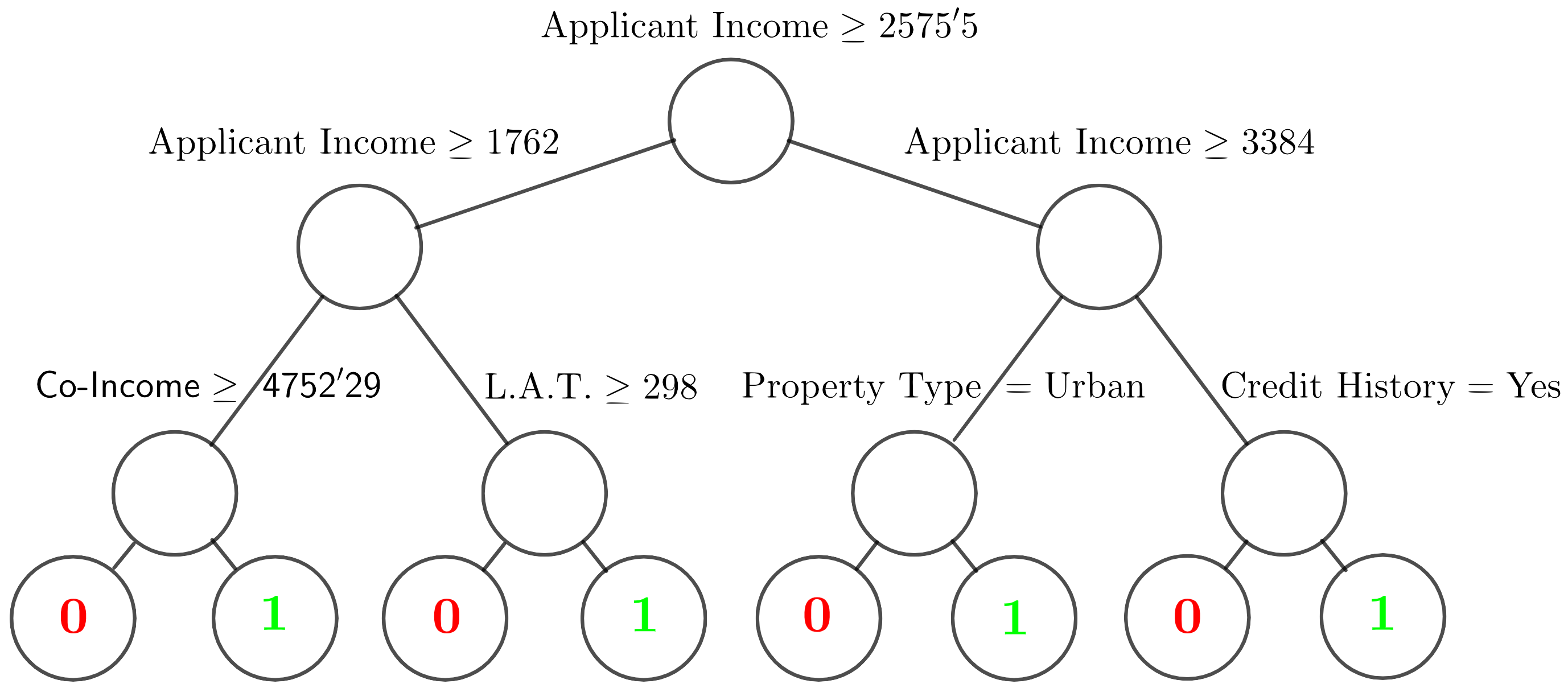
Figure 4. Solution OCT ($\sim 78\%$ of acccuracy) for the Mortgage case study.

   

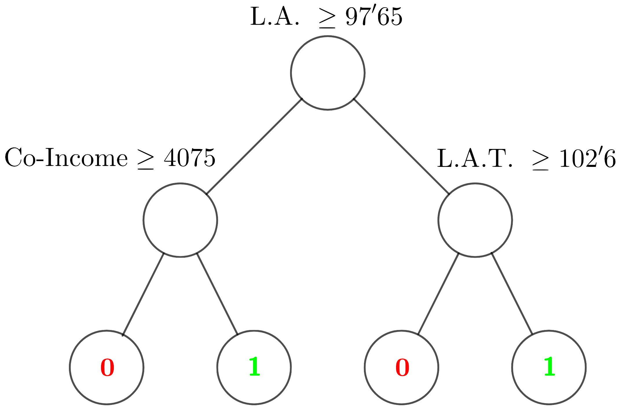
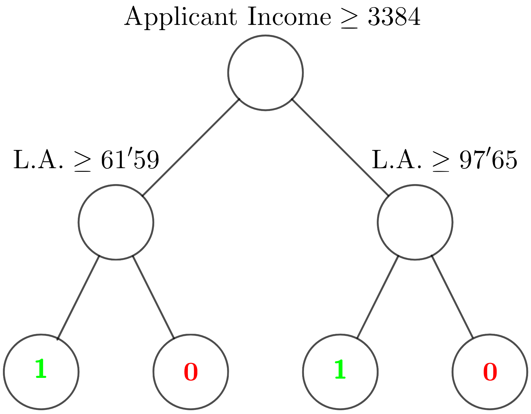
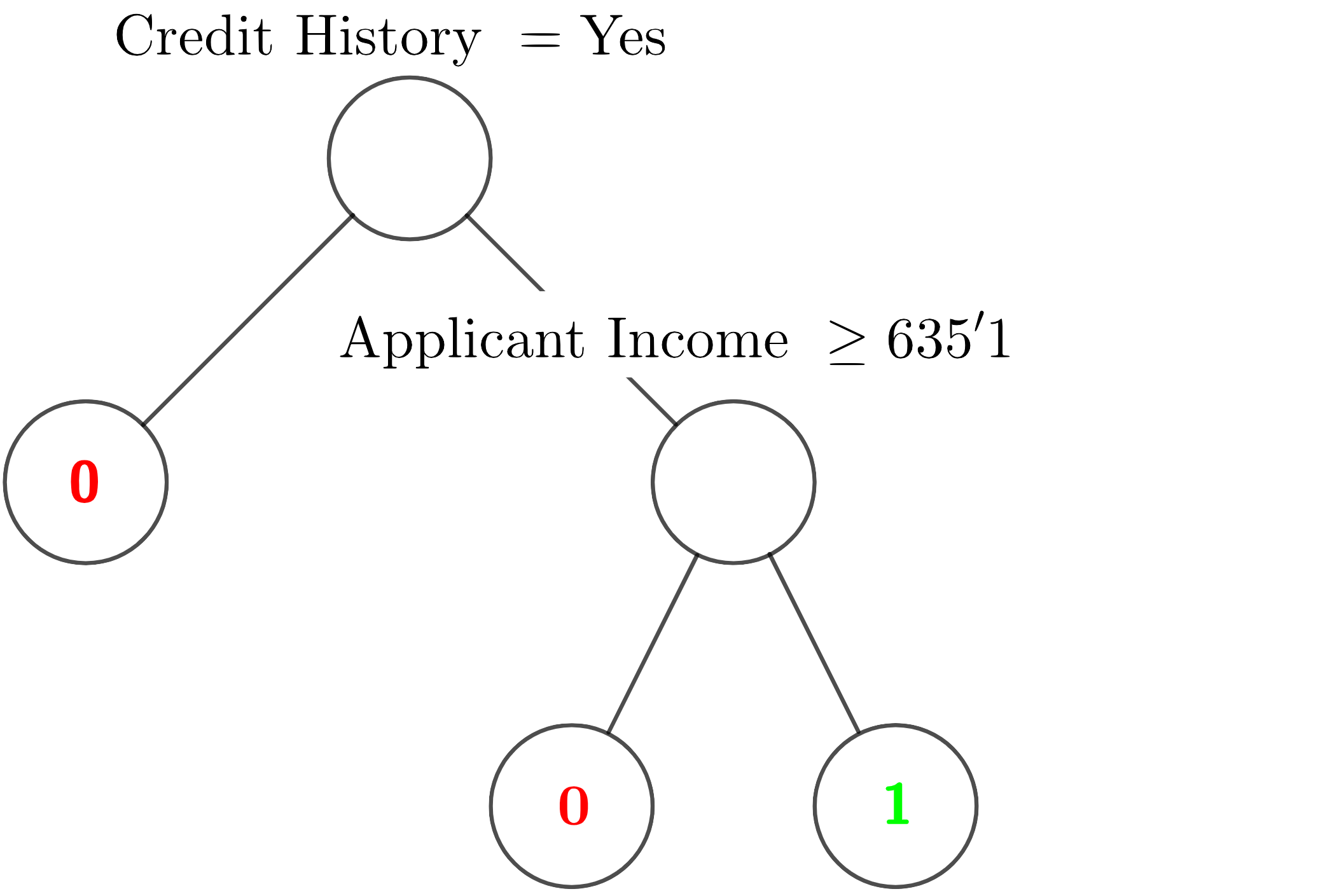
Figure 5. Solution 3-OCF ($\sim 82\%$ of accuracy) for the Mortgage case study.

In the solution provided by OCT, the income variable is used in the first levels to derive the classification rule. In particular, the first split is built very close to the value of the first quartile of the income variable ($Q_{1}=2899$), and therefore, the L.A. and mainly L.A.T. variables, which is where we have the room for maneuver, will only affect to less than $25\%$ of the potential clients, while more than $75\%$ of potential clients will have no option to be recovered out from the ungranted set of clients. On the other hand, if we look at the solution provided by the 3-OCF, we find that one of the trees contains a branch that depends only on the variables L.A and L.A.T. Thus, the company will always have the option of calibrating these values to give a positive vote to a client, which, although will not ensure that the loan will be granted (the client must obtain at least $2$ out of $3$ votes to be granted), will increase its probability for all the clients. In fact, combining this branch with the credit history branch linked to having a minimum income allows for a lot of flexibility to end up granting a loan. In conclusion, in this case, the 3-OCF model not only provides a higher accuracy ($\sim 82\%$) than OCT ($\sim 78\%$), but also a more flexible solution for the company and the clients.

Although, as expected, the applicant income is a crucial variable to determine whether a client is granted, this is adequately combined with other variables (as L.A., L.A.T, Co-Income and Credit History) to alleviate negative values in one of the trees with positive values in the remainder trees. For instance, this might be the case of a client applyinh for a L.A. greater than 61.59, but with incomes smaller than $\$3385$. The second tree rejects the loan to this client. Nevertheless, in case the co-incomes are greater than $4075$, the first tree will accept the loan. Furthermore, if this client has a credit history and the client’s incomes are greater than $635.1$, the third tree will also accept the loan. By majority, the client will get the loan. The solution obtained by OCT, for the same client with incomes smaller than $\$3384$, would grant the loan only if it is used to pay an urban property. Otherwise, the loan will not be accepted.

5.2. Case Study 2: Hotel reservations

In our second case study, we analyze one of the datasets provided in Antonio et. al (2019). In such a work they present and study two datasets containing information on a series of room bookings in two hotels through the Booking company. In particular, we work with the first dataset which contains the information of a resort hotel, gathering $40060$ observations and $31$ variables, which cover all kinds of details about the customer’s reservation. In the following, we describe the variables that have been used in the models we have chosen (the interested reader is referred to Antonio et. al (2019) for further details on the variables defining the dataset):

• Reservation Status: Takes value 1 if the reservation is canceled and value 0 otherwise

• Room Type: Categorical variable

• ADR: Average Daily Rate (total price paid by the customer divided by the number of nights)

• Lead Time: Number of days elapsed between the date of entry of the booking and the date of arrival

• TSR: Total number of Special Requests of the room by the customer

• Parking: Takes value 1 if the customer asks for a parking space and value 0 otherwise

The goal of this study is to decide whether a customer is susceptible to cancel a hotel reservation or not. In this way, the hotel desires to construct a classification rule to determine the reliability of a customer when making the reservation. However, as in the previous case study, once a classification model has been trained, the hotel has some room for tweaking some of the variables, such as the room price, and could thus obtain more robust bookings from its customers (for example, a better adjustment on the pricing could cause a customer to no longer be classified as a potential cancellation but as a potential booking).

In our problem, the variable Room Type has not been used as a predictor variable but as a filter one. We made this decision because of its categorical nature and decided to focus on the $966$ type-6 room reservations. These rooms have on average the highest average cost per night, and also the highest imbalance in the target variable, i.e., the highest percentage of cancellations ($45\%$). Next, as done in the previous case study, we present the solutions provided by $3$-OCF and OCT for the problem, which have been obtained as in the previous case by following the train-validation-test partition schedule.

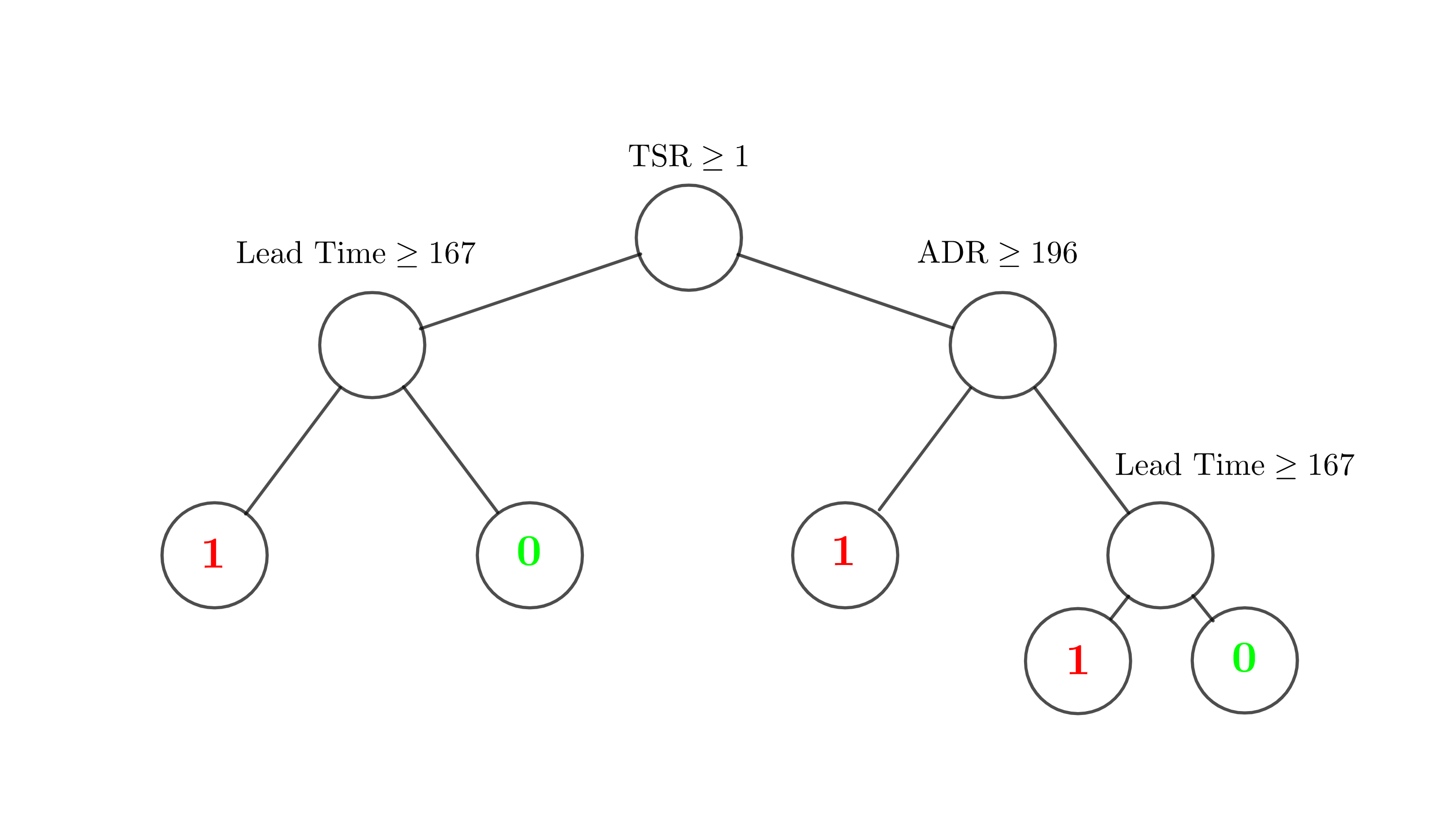
Figure 6. Solution OCT ($\sim 89\%$ of accuracy) for the Booking dataset.

   

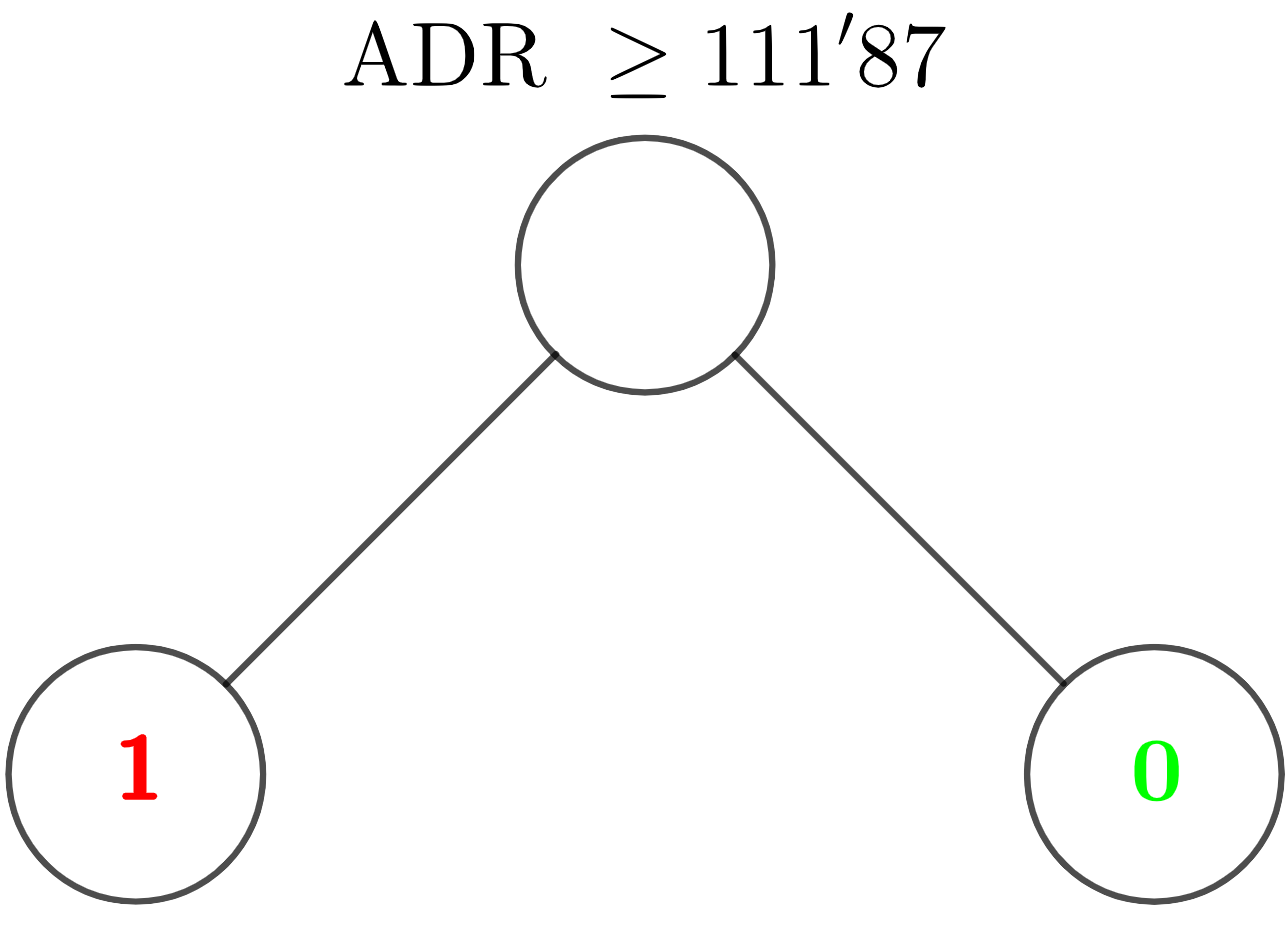
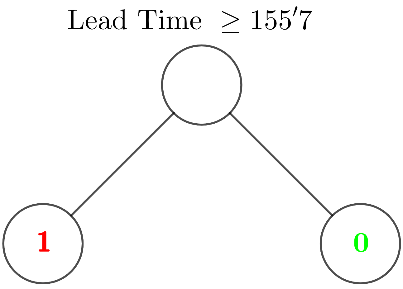
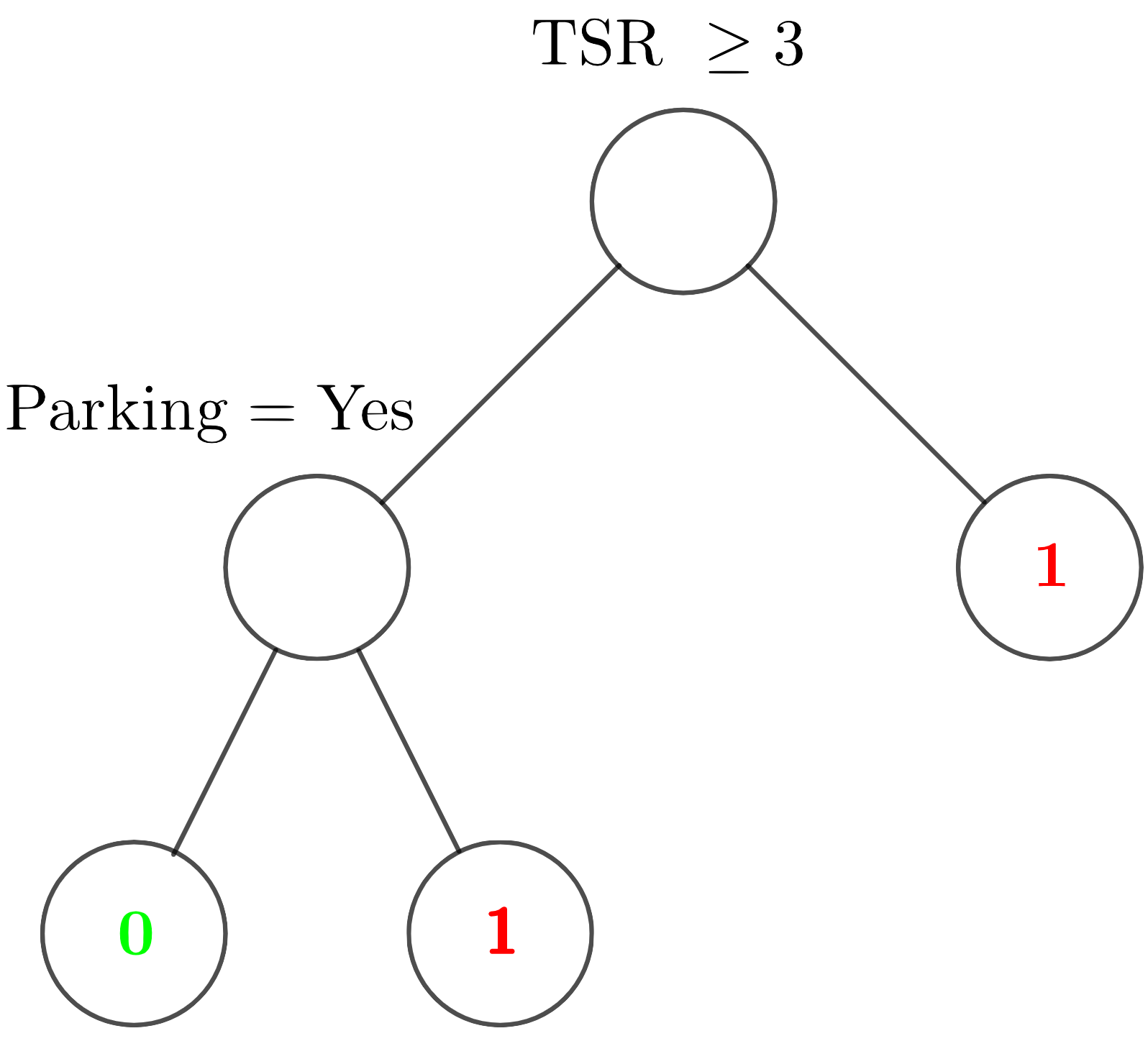
Figure 7. Solution 3-OCF ($\sim 89\%$ of accuracy) for the Bookng dataset.

In this case, both model have exactly the same performance in terms of accuracy in the test set ($\sim 87\%$) and both are easily interpretable. The OCT model starts by differentiating between the most demanding customers (given that we are dealing with the most expensive rooms in the hotel, it is to be expected that guests may have more specific requirements), and then takes into consideration the variables of price and lead time. In contrast, the 3-OCF model separates the price and lead time variables independently into two trees, and leaves a third tree to differentiate the most demanding customers, making a small distinction between those who ask for parking and those who do not (note that asking for parking implies that the customer has independence of movement and is, therefore, more likely to cancel and stay in other locations).

Thus, 3-OCF only automatically discards customers who book at a short advance and have a high number of special requests, whereas for the rest it will be able to adjust the price and maximize the hotel’s bookings. On the other hand, the price variable in the OCT model can only be readjusted for a smaller subset of potential customers. Therefore, the $3$-OCF model provides more flexibility for the hotel to manage bookings successfully.

5.3. Case Study 3: Airlines satisfaction problem

In the previous two cases, we have seen the advantages that can be gained in terms of interpretability and flexibility by using 3-OCF for small/medium data sets. In this last case, we show that this methodology can also be applied to large datasets and still obtain advantageous results in interpretability. In particular, we will analyze one of Kaggle’s public datasets: Airline Passenger Satisfaction. The page itself invites to use of a set of $103,904$ observations and $25$ variables as training validation, and another $30,000$ observations as a test. We have used two-thirds of the training-validation observations for the downsampling procedure, and subsequent training of the model has been done. The remaining third of the observations have been used for validation while maintaining the proposed test observations.

The goal here is to determine, from the given dataset, whether a person is satisfied with an air travel experience ($44\%$ of the training sample) versus being dissatisfied or neutral ($56\%$ of the training sample). The $24$ predictor variables provide information about the customer and the flight itself. Below, as in the previous cases, we describe the variables that have been involved in our chosen models, the reader can find the details of the other variables in the Kaggle link:

• Satisfaction: takes value 1 if the customer is satisfied with the travel and takes value 0 otherwise

• Online Boarding: satisfaction with respect to the onlinea boarding (from 0 to 5)

• Wifi: satisaction with respect to the inflight wifi service (from 0 to 5)

• Service: satisaction with respect to the inflight service (from 0 to 5)

• Gate: satisaction with respect to the gate location (from 0 to 5)

• Age: Continuous variable

• Type: Business / Personal

The solutions obtained for this dataset are graphically shown in figures 8 (OCT) and 9 (OCF). As can be observed, both methods obtain a similar accuracy in the test set (around $89\%$). Interestingly, in this case, the three trees obtained by 3-OCF provide information about three differentiated elements, that combined produce high accuracy. In the first tree, the first split differentiates customers by age. The younger customers rate positively the trip if the plane has a good wifi system, whereas older customers, instead, take into account the inflight service to provide a positive rate. The second tree only gives a negative vote when the reason for the trip is personal and the customer is unsatisfied with the boarding gate, i.e., when the process of finding the gate and getting on the plane has not been smooth. In contrast, for business trips this is not a relevant factor and in general a positive vote is given. Finally, the third tree gives a positive vote if the online boarding system has been satisfactory. On the other hand, if we look at the solution proposed by OCT, although equally interpretable, the solution is not so clear at first sight. For example, we can see that the wifi variable is involved in different branches at different depths with different cut-off values, which may be less intuitive to analyze.

In conclusion, for this dataset, 3-OCF outputs three trees modeling different aspects of the satisfaction of airline trips, that seem more favorable than the one provided by the OCT, where following deeper branches with duplicated variables can make the interpretation a lot more confusing.

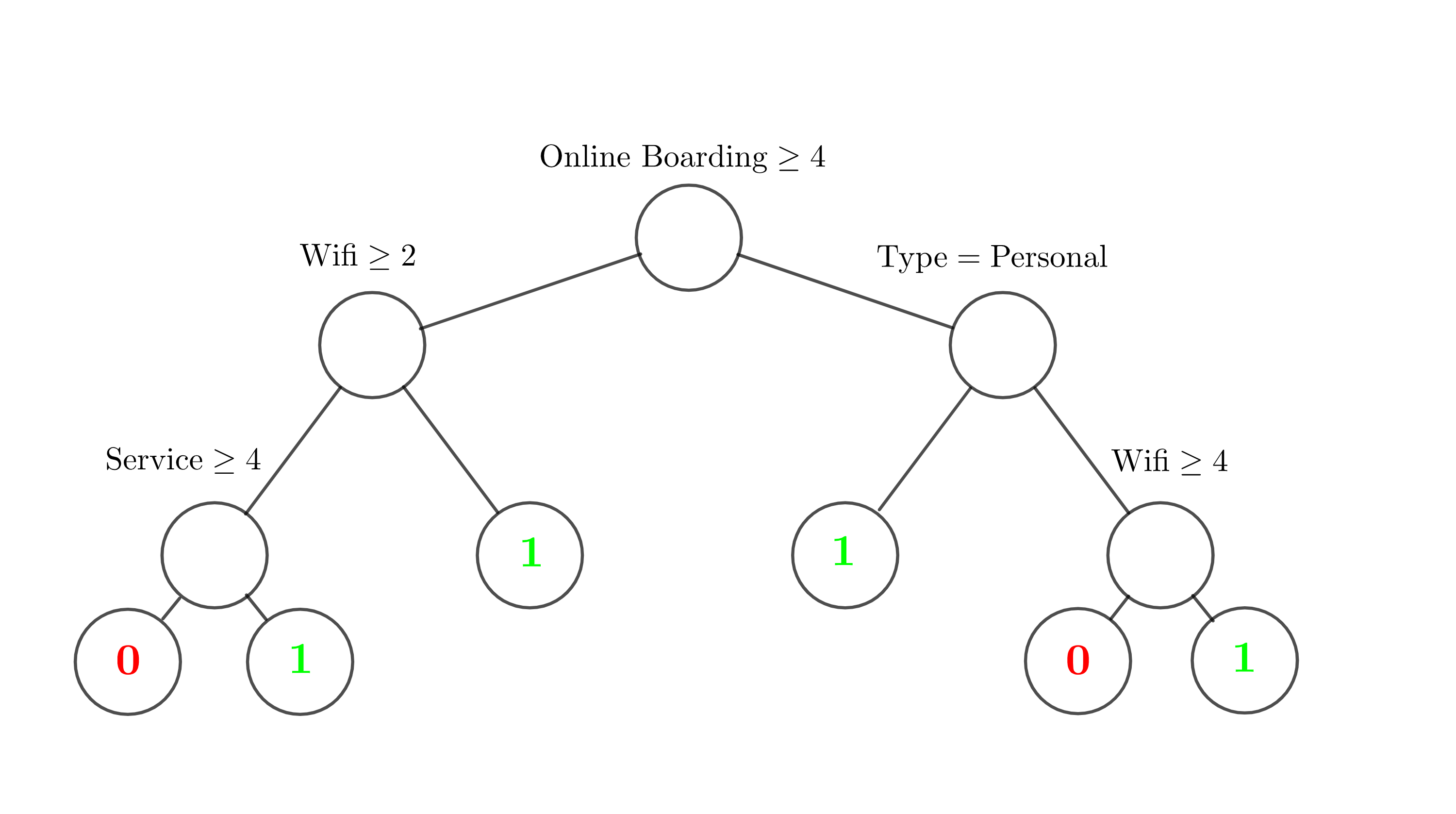
Figure 8. Solution OCT ($\sim 89\%$ of accuracy) for the airline dataset.

   

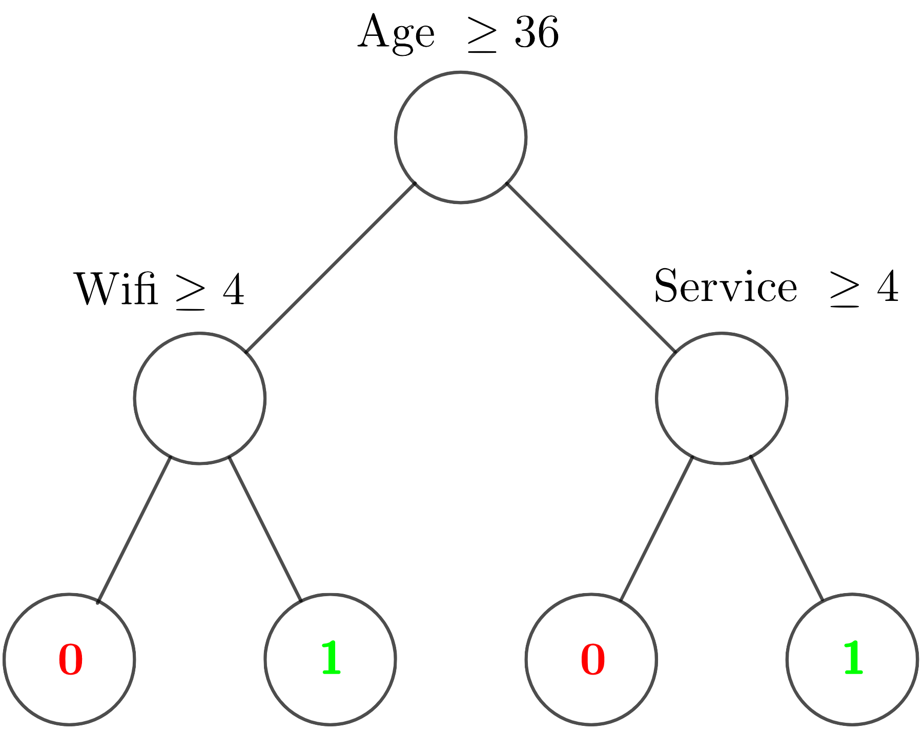
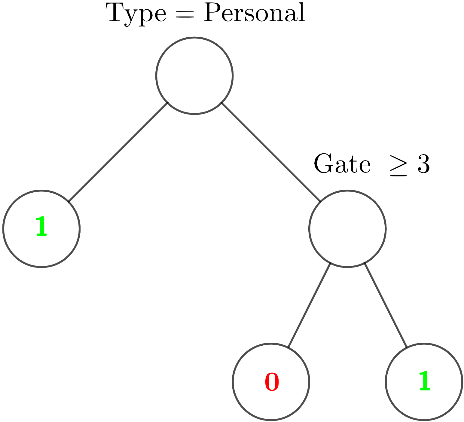
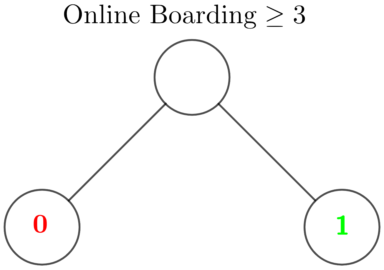
Figure 9. Solution 3-OCF ($\sim 89\%$ of accuracy) for the airline dataset.

6. Conclusions

We propose here a new supervised classification method based on a voting-by-label process from a forest of classification trees. The decision rule is obtained by solving a mixed integer linear program on the training sample. Therefore, as this is a complex combinatorial optimization problem, the results have been tested on a series of well-known rather small to medium-sized datasets, outperforming some existing tree-based methods (CART and OCT) in terms of accuracy and obtaining results comparable to a random forest with a much larger number of trees by using a small amount of them. Moreover, we present some successful ideas to facilitate model training such as downsampling strategies or symmetry breaking constraints. Finally, we show through three real case studies how OCF solutions are not only easily interpretable but also more flexible than those provided by other CT-based methods.

This is the first step in the study of this methodology, and a promising entry point for future work in tackling larger problems. In view of the results, there is still room for improvement of OCF in different directions. A deep analysis of the mathematical optimization problem that we propose would lead us to enhance its computational performance by finding valid inequalities, deriving strategies for fixing variables of the model, or designing decomposition approaches for solving larger-size training instances with less computational time.

References

- Baldomero-Naranjo et. al (2020) Baldomero-Naranjo M, Martínez-Merino LI, Rodríguez-Chía AM (2020) Tightening big ms in integer programming formulations for support vector machines with ramp loss. European Journal of Operational Research 286(1):84–100
- Baldomero-Naranjo et. al (2021) Baldomero-Naranjo M, Martínez-Merino LI, Rodríguez-Chía AM (2021) A robust svm-based approach with feature selection and outliers detection for classification problems. Expert Systems with Applications 178:115,017
- Benítez-Peña et. al (2019) Benítez-Peña S, Blanquero R, Carrizosa E, et al (2019) Cost-sensitive feature selection for support vector machines. Computers & Operations Research 106:169–178
- Bertsimas and Dunn (2017) Bertsimas, D., and Dunn, J. (2017). Optimal classification trees. Machine Learning, 106(7), 1039-1082.
- Bertsimas et. al (2022) Bertsimas, D., Dunn, J., and Paskov, I. (2022). Stable Classification. Journal of Machine Learning Research, 23(296), 1-53.
- Biau and Scornet (2016) Biau, G., and Scornet, E. (2016). A random forest guided tour. Test, 25(2), 197-227.
- Blanco et. al (2021) Blanco, V., Japón, A., and Puerto, J. (2021). Multiclass optimal classification trees with svm-splits. arXiv preprint arXiv:2111.08674.
- Blanco et. al (2020a) Blanco, V., Japón, A., and Puerto, J. (2020). Optimal arrangements of hyperplanes for SVM-based multiclass classification. Advances in Data Analysis and Classification, 14(1), 175-199.
- Blanco et. al (2020b) Blanco, V., Puerto, J., and Rodriguez-Chia, A. M. (2020). On lp-support vector machines and multidimensional kernels. The Journal of Machine Learning Research, 21(1), 469-497.
- Blanco et. al (2022) Blanco, V., Japón, A., and Puerto, J. (2022). Robust optimal classification trees under noisy labels. Advances in Data Analysis and Classification, 16(1), 155-179.
- Blanquero et. al (2021) Blanquero R, Carrizosa E, Molero-Río C, et al (2021) Optimal randomized classification trees. Computers & Operations Research 132:105,281
- Breiman (1996) Breiman, L. (1996). Bagging predictors. Machine learning, 24, 123-140.
- Breiman (2001) Breiman, L. (2001). Random forests. Machine learning, 45(1), 5-32.
- Breiman et. al (1984) Breiman L, Friedman J, Olshen R, et. al (1984) Classification and regression trees
- Carreira-Perpiñán and Tavallali (2018) Carreira-Perpiñán MA, Tavallali P (2018) Alternating optimization of decision trees, with application to learning sparse oblique trees. In: Proceedings of the 32nd International Conference on Neural Information Processing Systems. Curran Associates Inc., Red Hook, NY, USA, NIPS’18, pp 1219–1229
- Carrizosa et. al (2021) Carrizosa, E., Molero-Río, C., and Romero Morales, D. (2021). Mathematical optimization in classification and regression trees. Top, 29(1), 5-33.
- Chen and Guestrin (2016) Chen, T., and Guestrin, C. (2016, August). Xgboost: A scalable tree boosting system. In Proceedings of the 22nd acm sigkdd international conference on knowledge discovery and data mining (pp. 785-794).
- Demirović et. al (2022) Demirović E, Lukina A, Hebrard E, et al (2022) Murtree: Optimal decision trees via dynamic programming and search. Journal of Machine Learning Research 23(26):1–47
- Eitrich and Lang (2006) Eitrich T, Lang B (2006) Efficient optimization of support vector machine learning parameters for unbalanced datasets. Journal of computational and applied mathematics 196(2):425–436
- Firat et. al (2020) Firat M, Crognier G, Gabor AF, et al (2020) Column generation based heuristic for learning classification trees. Computers & Operations Research 116:104,866
- Gan et. al (2021) Gan J, Li J, Xie Y (2021) Robust svm for cost-sensitive learning. Neural Processing Letters pp 1–22
- Günlük et. al (2021) Günlük, O., Kalagnanam, J., Li, M., Menickelly, M., and Scheinberg, K. (2021). Optimal decision trees for categorical data via integer programming. Journal of Global Optimization, 81, 233-260.
- Hu et. al (2019) Hu X, Rudin C, Seltzer M (2019) Optimal sparse decision trees. Advances in Neural Information Processing Systems 32
- Hu et. al (2020) Hu H, Siala M, Hebrard E, et al (2020) Learning optimal decision trees with maxsat and its integration in adaboost. In: IJCAI-PRICAI 2020, 29th International Joint Conference on Artificial Intelligence and the 17th Pacific Rim International Conference on Artificial Intelligence
- Lichman (2013) Lichman, M. (2013). UCI machine learning repository.
- Lin et. al (2020) Lin J, Zhong C, Hu D, et al (2020) Generalized and scalable optimal sparse decision trees. In: International Conference on Machine Learning, PMLR, pp 6150–6160
- Murthy et. al (1994) Murthy SK, Kasif S, Salzberg S (1994) A system for induction of oblique decision trees. J Artif Int Res 2(1):1–32
- Narodytska et. al (2018) Narodytska N, Ignatiev A, Pereira F, et al (2018) Learning optimal decision trees with sat. In: Ijcai, pp 1362–1368
- Antonio et. al (2019) Antonio, N., de Almeida, A., and Nunes, L. (2019). Hotel booking demand datasets. Data in brief, 22, 41-49.
- Quinlan (1996) Quinlan J (1996) Machine learning and id3. Los Altos: Morgan Kauffman
- Quinlan (1993) Quinlan R (1993) C4. 5. Programs for machine learning
- Rudin et. al (2022) Rudin, C., Chen, C., Chen, Z., Huang, H., Semenova, L., and Zhong, C. (2022). Interpretable machine learning: Fundamental principles and 10 grand challenges. Statistics Surveys, 16, 1-85.
- Cortes and Vapnik (1995) Cortes C, Vapnik V (1995) Support-vector networks. Machine learning 20(3):273–297
- Mišić (2020) Mišić, V. V. (2020). Optimization of tree ensembles. Operations Research, 68(5), 1605-1624.
- Verhaeghe et. al (2020) Verhaeghe H, Nijssen S, Pesant G, et al (2020) Learning optimal decision trees using constraint programming. Constraints 25(3):226–250
- Verwer and Zhang (2019) Verwer S, Zhang Y (2019) Learning optimal classification trees using a binary linear program formulation. In: Proceedings of the AAAI conference on artificial intelligence, pp 1625–1632
- Yu et. al (2020) Yu J, Ignatiev A, Stuckey PJ, et al (2020) Computing optimal decision sets with sat. In: International Conference on Principles and Practice of Constraint Programming, Springer, pp 952–970