Iterative Qubit Coupled Cluster using only Clifford circuits

Abstract

We draw attention to a variant of the iterative qubit coupled cluster (iQCC) method that only uses Clifford circuits. The iQCC method relies on a small parameterized wave function ansatz, which takes form as a product of exponentiated Pauli word operators, to approximate the ground state electronic energy of a mean field reference state through iterative qubit Hamiltonian transformations. In this variant of the iQCC method, the wave function ansatz at each iteration is restricted to a single exponentiated Pauli word operator and parameter. The Rotosolve algorithm utilizes Hamiltonian expectation values computed with Clifford circuits to optimize the single-parameter Pauli word ansatz. Although the exponential growth of Hamiltonian terms is preserved with this variation of iQCC, we suggest several methods to mitigate this effect. This method is useful for near-term variational quantum algorithm applications as it generates good initial parameters by using Clifford circuits which can be efficiently simulated on a classical computers according to the Gottesman–Knill theorem. It may also be useful beyond the NISQ era to create short-depth Clifford pre-optimized circuits that improve the success probability for fault-tolerant algorithms such as phase estimation.

I Introduction

There are many flavours of Variational Quantum Algorithms (VQA) [1, 2, 3, 4, 5, 6] to determine the states and energies for a given system. In VQA, a parameterized ansatz is chosen to describe one or more eigenvectors of a qubit Hamiltonian $\hat{H}=\sum_{j}h_{j}P_{j}$, where $\quad P_{j}=\otimes_{k=1}^{N}\sigma_{k}^{(j)}$ is a Pauli word operator formed as a tensor product of Pauli and identity operators $\sigma_{k}^{(j)}\in[X,Y,Z,I]$, $N$ is the number of qubits, and $h_{j}$ is an expansion coefficient. For fermionic systems, the set of coefficients $h_{j}$ are derived from the one- and two-electron integrals of a second-quantized Hamiltonian using any of the popular mappings such as Jordan-Wigner (JW), Bravyi-Kitaev (BK), and JKMN [7] (also known as the ternary-tree mapping). A qubit Hamiltonian expectation value is determined on a quantum computer by first preparing an initial qubit state according to the chosen ansatz and current parameter set, then applying each $P_{j}$ term individually or as groups of mutually commuting $P_{j}$ terms, and finally measuring the final qubit state. Minimization of this expectation value with respect to the ansatz parameters is performed on a classical computer and affords the optimal energy and parameter set for the selected ansatz. An effective ansatz will navigate towards the optimal solution with short depth circuits, and a minimal number of parameters.

A promising wave function ansatz for VQA applications is qubit coupled cluster (QCC) [1, 2]. This method utilizes a parameterized ansatz $\hat{U}_{\rm{QCC}}$ that is expressed as a product of exponentiated Pauli words, $\hat{U}_{\rm{QCC}}=\prod^{M}_{j=1}{{\rm{exp}}\left(-\frac{i}{2}\tau_{j}\mathcal{P}_{j}\right)}$, where $M$ is the number of $\mathcal{P}_{j}$ operators used in the ansatz, $\quad\mathcal{P}_{j}=\otimes_{k=1}^{N}\sigma_{k}^{(j)}$, $\sigma_{k}^{(j)}\in[X,Y,Z,I]$, and $\tau_{j}\in[0,2\pi)$. It is noted that the set of $\mathcal{P}_{j}$ operators appearing in $\hat{U}_{\rm{QCC}}$ is distinct from the set of $P_{j}$ operators present in $\hat{H}$. For a system of $N$ qubits, the number of candidate $\mathcal{P}_{j}$ operators to consider for the QCC ansatz is $N_{\mathcal{P}}=4^{N}$, and utilization of all candidates in $\hat{U}_{\rm{QCC}}$ provides a formally exact wave function representation for a qubit Hamiltonian.

It was recognized in Ref. [2] that Pauli $Z$ operators do not contribute to variational energy lowering. Thus, for each $\mathcal{P}_{j}$ in $\hat{U}_{\rm{QCC}}$, $\sigma_{k}^{(j)}\in[X,Y,I]$, and the number of candidate $\mathcal{P}_{j}$ operators is reduced to $N_{\mathcal{P}}=3^{N}$. Interestingly, the choice of mapping influences the number of candidate operators to consider for the QCC ansatz. In previous studies of QCC-based methods [1, 2], restricting the rank of candidate operators, which is denoted as $\lvert\mathcal{P}_{j}\rvert$ and is a count of the number of Pauli operators, was proposed as a route to systematically control the problem complexity and accuracy of the solution. In Refs. [1, 2] where the JW and BK mappings were considered, it is noted that the rank of candidate operators respects $2\leq\lvert\mathcal{P}_{j}\rvert\leq N$. In addition to the JW and BK mappings, we employed for the first time to our knowledge the JKMN mapping for the QCC ansatz in VQA applications. It was found for the JKMN mapping that candidate $\mathcal{P}_{j}$ operators for the QCC ansatz must respect $1\leq\lvert\mathcal{P}_{j}\rvert\leq N$ to achieve convergence of the total electronic energy.

It was noted in Ref. [2], and later in Ref. [5], that candidate Pauli words require an odd number of Pauli $Y$ operators, which we found can also hold true for the JKMN mapping if the Majorana mode representations are chosen carefully. Piecing together the observations discussed above affords a lower bound for the pool size of candidate Pauli words to consider for the QCC ansatz as

$$N_{\mathcal{P}}=\sum^{N}_{\begin{subarray}{c}n_{y}=1\\ n_{y}{\rm{odd}}\end{subarray}}{\sum^{N-n_{y}}_{n_{x}=n_{0}}{{N\choose n_{y}}{N-n_{y}\choose n_{x}}}}\;.$$ (1)

In Eq. 1, $n_{x}$ and $n_{y}$ are the number of Pauli $X$ and $Y$ operators present in the candidate operator, $n_{0}=1$ for the JW and BK mappings, and $n_{0}=0$ for the JKMN mapping.

One can efficiently generate $N_{\mathcal{P}}$ candidate $\mathcal{P}_{j}$ operators by utilizing the flip index procedure described in Ref. [2], which comes at a cost that scales linearly with the number of qubit Hamiltonian terms. Flip indices correspond to the indices where Pauli $X$ and $Y$ operators appear in each qubit Hamiltonian term $P_{j}$. It is shown in Ref. [2] that energy-lowering Pauli word candidates for the QCC ansatz require Pauli $X$ and $Y$ operators to be present at the flip indices. Since the Pauli $Z$ operators do not offer variational advantage for the QCC ansatz, identity matrices are placed at all non-flip indices when constructing candidate $\mathcal{P}_{j}$ operators without sacrificing accuracy of the ground state solution. For each unique set of flip indices, a set of candidate Pauli words is formed by placing all combinations of Pauli $X$ and $Y$ operators at the flip indices and $I$ matrices everywhere else such that each operator has an odd number of Pauli $Y$ operators and respects the minimum Pauli word rank determined by the chosen mapping. Using a representative Pauli word from each candidate set, the gradient of the QCC energy is evaluated to assess whether operators from this candidate set can offer variational advantage for the QCC ansatz.

The set of energy-lowering Pauli word candidates obtained from the protocol described above is referred to as the direct interaction set (DIS) [2] and is denoted $\left\{\mathcal{P}\right\}$ below. Each element $\mathcal{P}_{j}$ from $\left\{\mathcal{P}\right\}$ can be exponentiated with a rotational parameter $\phi_{j}$ to form a generator $\mathcal{G}_{j}=\exp\left(-\phi_{j}\mathcal{P}_{j}\right)$. After $M$ unique generators are created and applied sequentially in the circuit, the ansatz is optimized as with any other VQA. Another QCC iteration can be applied by folding the generators into the Hamiltonian. The following equation,

$$\begin{array}[]{ccr}\hat{H}_{m}&=&\hat{H}_{m+1}+\frac{1}{2}\big{[}\big{(}1-\cos\left(\phi_{m}\right)\big{)}\mathcal{P}_{m}-i\sin(\phi_{m})\big{]}\times\\ &&\left[\hat{H}_{m+1},\mathcal{P}_{m}\right],\end{array}$$ (2)

is applied for each generator in reverse order of the appearance in the circuit such that $\hat{H}_{M+1}$ is the original Hamiltonian and $\hat{H}_{0}$ is the Hamiltonian used for the next QCC step. This is referred to as the iterative qubit coupled cluster [2] (iQCC) approach.

The optimization of parameters in VQA does have well-known problems. First, ansatz expressivity often comes at the cost of trainability, due to the occurrence of barren plateaus [8, 9]. The iterative nature of iQCC aims to mitigate this problem by avoiding long depth circuits with many parameters. Still, large expectation value variances can be present in the Hamiltonian [10] when measuring term-by-term or in commuting groups. Therefore, many measurements in many different measurement bases are required to obtain accurate results. This additional obstacle in VQAs is commonly known as the measurement problem. A technique to mitigate this problem is to start with a good initial guess to the optimal parameters, which minimizes the number of ansatz optimization steps required to converge to the correct answer. Several methods to find the best initializations have been proposed by using Clifford versions of the ansatz (quadratic Clifford expansion [11], Clifford circuit annealing [12], and Clifford Ansatz For Quantum Accuracy (CAFQA) [13]). The success of Clifford pre-optimization relies on the resulting stabilizer state having non zero expectations with the Pauli terms in the cost function, i.e, it returns useful information. This makes it more likely to be useful for Hamiltonians with many non-commuting groups [12].

Here, we present an algorithm that inherits the advantages of iQCC while avoiding the measurement problem by utilizing Clifford circuits. This is done by observing that the exponential of a Pauli word is composed of only Clifford gates for rotations $\pm\pi/2$ as compiled to a circuit using Reference 14, and that these are also the angles required for one Rotosolve [15] step. As Clifford circuits can be classically simulated [16], we can obtain exact optimal parameters and energies for every candidate Pauli word and choose the one that lowers the energy the most at each iteration without utilizing a quantum computer. Each chosen Pauli word is then folded into the Hamiltonian using Eq. (2) and the process is repeated until convergence. No quantum computing resources are required to implement this algorithm as it is performed completely classically. A reasonable approximation to the solution is obtained using the calculated sets of $\mathcal{P}_{m}$ and $\phi_{m}$ as shown by the convergence properties in the Examples section.

We propose iQCC as a strong method for Clifford pre-optimization. At each iteration the number of parameters remains small, and the number of Pauli terms grows exponentially. This exponential growth is normally detrimental for the iQCC method to be implemented on a quantum computer, but can be advantageous in the Clifford pre-optimization on a classical computer due to the increase in non-commuting (and non-zero) terms. Fortunately, when the final optimization across the whole circuit is preformed on a quantum computer, this can be done with the full circuit and the original qubit Hamiltonian to circumvent measuring an exponential number of terms on hardware.

II Algorithm

The algorithm begins with the generation of a Hamiltonian in the form of a qubit operator and the corresponding Hartree-Fock reference state. In QCC, a quantum mean field QMF [1] state is chosen. This can be initialized to the same as the Hartree-Fock reference but also can include other $Rx$ or $Rz$ rotations. For this algorithm, we require that the QMF state use only Clifford gates. This means that only rotation angles that are multiples of $\frac{\pi}{2}$ are permitted. For the purposes of this work, we restrict ourselves to the Hartree-Fock reference state which has all $Rz$ angles zero and $Rx$ angles of $0$, $\pi$ depending on the orbital occupations and the chosen mapping. In this work, it is not necessary to use a QMF starting state. The only requirement is that the preparation circuit ($C_{prep}$) representing the initial reference state is composed only of Clifford gates. This means that one could utilize the other Clifford initialization techniques [11, 12, 13] and proceed with no further changes to the algorithm.

After the reference QMF circuit and initial qubit Hamiltonian ($\hat{H}$) are generated. The steps are as follows. 1) Calculate the starting energy $E$ using established methods [17]. 2) Generate $\mathcal{P}$, the DIS of energy-lowering candidate Pauli words described in Ref. [2]. 3) For each candidate Pauli word, a) generate Clifford circuits corresponding to $\pm\pi/2$ using the CNOT ladder construction of Reference 14. Clifford decompositions for the necessary operations are

$$\begin{array}[]{lcl}Rz(\pi/2)&=&HS^{\dagger}HS^{\dagger}H\\ Rz(-\pi/2)&=&HSHSH\\ Rx(\pi/2)&=&S^{\dagger}HS^{\dagger}\\ Rx(-\pi/2)&=&SHS\end{array}$$ (3)

where $H$ is the Hadamard Gate and $S$ is the phase gate $\sqrt{Z}$. b) Use the Rotosolve equations to calculate the exact minimum (and corresponding rotation angle) for that generator. This is done by

$$\begin{array}[]{rcl}\phi_{min}&=&-\frac{\pi}{2}-\mbox{arctan2}\left(2E-\left<\hat{H}\right>_{\pi/2}-\left<\hat{H}\right>_{-\pi/2},\left<\hat{H}\right>_{\pi/2}-\left<\hat{H}\right>_{-\pi/2}\right)\\ A&=&\frac{1}{2}\sqrt{\left(2E-\left<\hat{H}\right>_{\pi/2}-\left<\hat{H}\right>_{-\pi/2}\right)^{2}+\left(\left<\hat{H}\right>_{\pi/2}-\left<\hat{H}\right>_{-\pi/2}\right)^{2}}\\ B&=&\arctan 2\left(2E-\left<\hat{H}\right>_{\pi/2}-\left<\hat{H}\right>_{-\pi/2},\left<\hat{H}\right>_{\pi/2}-\left<\hat{H}\right>_{-\pi/2}\right)\\ C&=&\frac{1}{2}\left(\left<\hat{H}\right>_{\pi/2}+\left<\hat{H}\right>_{-\pi/2}\right)\\ E_{new}&=&A\sin\left(\phi_{min}+B\right)+C\end{array}$$ (4)

where $\left<\hat{H}\right>_{\phi}$ is the Hamiltonian $\hat{H}$ expectation value at angle $\phi_{min}$. When using a QMF state, one could calculate the expectation values by expanding the Hamiltonian using Eq. (2) with $\phi_{j}=\pm\pi/2$ and calculating the expectation value with the QMF reference using [17]. But this is most likely less efficient. 4) Select the generator $\mathcal{P}_{min}$ that minimizes the energy most. 5) Check if $E_{new}-E$ is less than some convergence criteria. Otherwise, set $E$ to $E_{new}$, and fold the exponentiated Pauli word into the circuit by Eq. 2 with $\phi_{m}=\phi_{min}$ and $\mathcal{P}_{m}=\mathcal{P}_{min}$. Return to step 2. Step 1 is already obtained by $E_{new}$. This process is shown in Algorithm 1.

Algorithm 1 Clifford iQCC algorithm for one iteration

$H_{0}$

Clifford reference state

obtain $\{\mathcal{P}_{j}\}$ from DIS of $H_{m}$

for all $\mathcal{P}_{j}$ in $\{\mathcal{P}_{j}\}$ do

     for $\phi$ in $\{\pi/2,-\pi/2\}$ do

         circuit $\leftarrow$ $e^{i\phi P_{j}}$

     end for

     $E_{\mathcal{P}_{j}}$, $\phi_{\mathcal{P}_{j}}$ $\leftarrow$ Rotosolve(circuit)

end for

SELECT $\mathcal{P}_{j}$ where $E_{min}=min\{E_{\mathcal{P}_{j}}\}$

$E_{m+1}=E_{min}$

$\mathcal{P}_{m+1}\leftarrow\mathcal{P}_{j}$

$\phi_{m+1}\leftarrow\phi_{j}$

if $E_{m+1}-E_{m}<\epsilon$ then

     Exit

end if

$m$ $\leftarrow$ $m+1$

generate $\hat{H}_{m+1}$ using all previous $\mathcal{P}_{m},\phi_{m}$

The complete circuit after all iterations can be compiled by applying the exponentiated Pauli words in reverse order (last operator to first) using the optimal angles generated. The expectation value of this circuit with the original qubit Hamiltonian will be equivalent to the final $E$. It should be noted that the parameters generated, although optimal at each step, are not optimal across the whole circuit. Further optimization on a quantum computer after each $\mathcal{P}_{m}$ is added would provide convergence to a desired accuracy in fewer iterations. This secondary optimization can be performed using the full circuit and the original Qubit Hamiltonian as the growth in the Hamiltonian makes the measurement problem more severe.

III Examples

Here, we present preliminary results for small systems. Although it is theoretically possible that this algorithm scales to very large systems, that is beyond the scope of this work as the exponential growth of the Hamiltonian is a problem that needs to be solved. As test systems, we choose the open-shell linear H₃ ($r=0.714A$) molecule in the STO-3G basis, the $(4,)$ fragment (the electrons in the 4th molecular orbital is active) of the MIFNO [18] decomposition of the HF molecule with ($r=0.9168$) in the 6-31g* basis as decomposed by QEMIST Cloud [19], and an isosceles trapezoid H₄ in the STO-3G basis with positions

$$\begin{array}[]{cccc}&x&y&z\\ H&1/\sqrt{2}&0&0\\ H&0&1/\sqrt{2}&0\\ H&-0.3-1/\sqrt{2}&0&0\\ H&0&-0.3-1/\sqrt{2}&0\end{array}$$ (5)

All calculations were performed using Tangelo [20], and the results have been compared to the respective Full Configuration Interaction (FCI) solutions. For all three systems, the Jordan-Wigner qubit mapping was used. As noted in reference 12, the chosen mapping determines where in the full N-qubit Hilbert space the ground state is located. We found the JKMN mapping often converged more slowly than Jordan-Wigner but Jordan-Wigner succeeded to high accuracy for all three systems tested. Bravyi-Kitaev reached similar accuracy in the same number of steps for H₃ and H₄ as Jordan-Wigner. For H₃, the Jordan-Wigner qubit mapping results in a 6-qubit problem. As shown in Figure 1(a), the accuracy is $10^{-9}$ after 20 iterations with no obvious plateaus. This shows that it may be possible to obtain arbitrary accuracy for a given system. Although the full HF problem requires $30$ qubits in the chosen $6-31G*$ basis, each fragment calculation requires fewer qubits with the $(4,)$ fragment only requiring $12$ qubits. As can be seen in Figure 1(b), accuracy of $10^{-4}$ Hartree for both the fragment energy and the reconstructed energy (of the full molecule) using FCI results for the other fragments is achieved after 8 iterations.

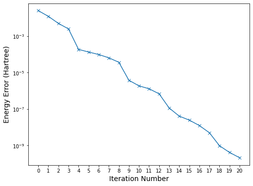
(a) Linear H₃

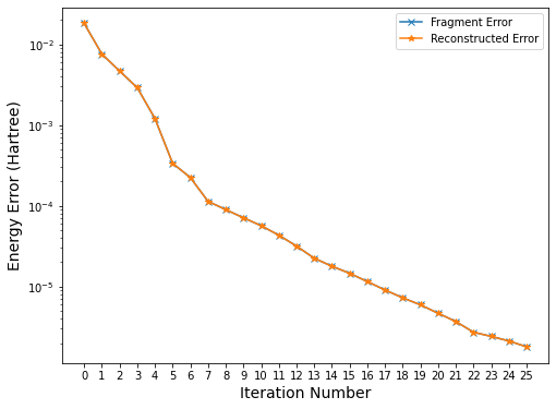
(b) (4,) fragment of HF

Figure 1: (a) After 20 iterations, the algorithm has obtain accuracy of around $10^{-9}$ for linear H₃ with inter-atomic distances ($r=0.714A$) with no sign of a barren plateau. (b) The MIFNO decomposed HF molecule with inter-atomic distance ($r=0.9168A$) converges to chemical accuracy in 4 iterations but we continue iterations to 25 to check for a barren plateau. This is not found. The reconstructed energy error using this fragment energy, with all the other fragment energies evaluated using QEMIST cloud, is of similar accuracy to the fragment error as shown in the plot.

In past work, the gradient was used to select generators [1]. We check whether it is worthwhile to perform the Clifford evaluations for all generators or to preselect the highest gradient and perform Rotosolve for the selected $\mathcal{P}_{j}$ only. In Figure 2(a), it is clear that faster convergence is achieved utilizing Rotosolve to select the generator that minimizes the energy most is beneficial. The number of terms in the Hamiltonian can increase faster using Rotosolve selection but the energy error for a given Hamiltonian size is always lower using Rotosolve to optimally select the next generator. This is shown in Figure. 2(b). The exponential scaling of the current algorithm is also evident by 2(b) linear convergence profile on a Log-Log plot.

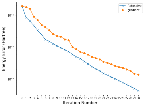
(a) H₄ energy convergence

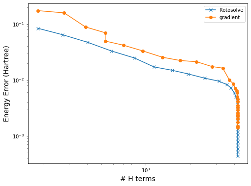
(b) H₄ energy error vs $\hat{H}$ terms

Figure 2: (a) The convergence of the energy by using gradient vs Rotosolve to select $\mathcal{P}_{m}$ for H₄ with trapezoid geometry. Selecting terms using Rotosolve converges faster. (b) The energy error vs the number of $\hat{H}$ terms. Rotosolve is always more efficient for a given accuracy. The vertical line occurs when the number of terms levels off at 4,216 which is much less than the theoretical maximum of 32,895.

IV Attenuating exponential growth of Hamiltonian terms

The main, and possible insurmountable, issue with this algorithm is the exponential growth in Hamiltonian terms that results from Eq. (2). Although it should first be noted that in practice, the number of Hamiltonian terms in iQCC seems to level off far below the maximum number of possible terms [21]. As shown in Figure 3(a), H₃ levels off at 282 terms which is far below the theoretical maximum of 2079 (max possible terms is $\sum_{m}^{\lfloor N/2\rfloor}\genfrac{(}{)}{0.0pt}{1}{N}{2m}3^{N-2m}$ [22]) however, this is probably due to the many symmetries of the linear H₃ molecule being C_∞v. As shown in Figure 3(b), the (4,) fragment of HF has 33,365 terms after 25 iterations with no signs of a barren plateau. This is far below the theoretical maximum of 8,390,655 Hamiltonian terms.

There are a few avenues that one may use to attenuate the expotential growth of qubit Hamiltonian terms. First, most of the Pauli words do not have support on the full Hamiltonian. It may be possible to restrict the DIS such that the rank of candidate Pauli words must be smaller than a particular value. In this case, one can compress the Hamiltonian by evaluating the expectation values of qubits not involved in the candidate Pauli word $\mathcal{P}_{m}$. With a Hartee-Fock reference state, any Hamiltonian term that measures the uninvolved qubits in the Pauli $X$ or $Y$ operator basis will have a zero expectation value, and so can be efficiently removed from the calculation. In fact, every chosen $\mathcal{P}_{m}$ acts on no more than 4 qubits for all three example calculations.

Another technique is to explore the possibility of adding multiple generators on the final step. As long as the added Pauli words commute, the order in which you add the generator does not affect the resulting circuit nor the transformed qubit Hamiltonian.

Finally, it may be possible to use involutory linear combinations (ILC) of mutually anti-commuting sets of Pauli word operators [22] to attenuate qubit Hamiltonian growth during the initial steps. The ILC procedure could also be performed as a pre-processing step before initializing Clifford iQCC as it is also classical pre-processing algorithm.

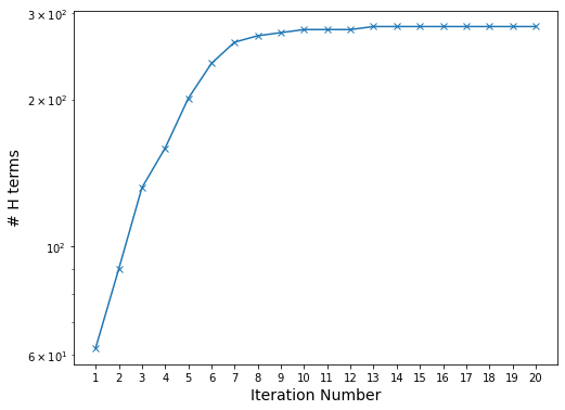
(a) H₃ $\hat{H}$ growth

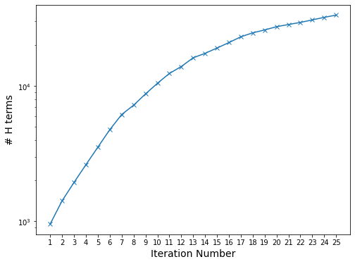
(b) HF $\hat{H}$ growth

Figure 3: The growth in the number of Hamiltonian terms with respect to the number of iQCC steps. (a) The number $\hat{H}$ terms for H₃ levels off at 282 terms which is much lower than the maximum number of 2079. (b) The number of terms in $\hat{H}$ for $(4,)$ of HF levels off around 40,000 terms which is much lower than the theoretical maximum of 8,390,655.

V Optimizing interior generators

It is possible to optimize interior generators and angles using Clifford circuits. To re-optimize $\phi_{m}$ for interior generator $\mathcal{G}_{m}$ selected at the $m$th iteration, one creates a qubit operator $Q_{m+1}=\sum_{q}c_{q}P_{q}$ that represents the action of the last $m+1$ to $M$ steps as

$$Q_{m+1}=\prod_{j=m+1}^{M}\left(\cos\left[\phi_{j}/2\right]-i\sin\left[\phi_{j}/2\right]\mathcal{P}_{j}\right),$$ (6)

and also calculates the folded Hamiltonian for the first $m-1$ steps (denoted $H_{m-1}=\sum_{j}h_{j}P_{j}$), which involves using Eq. (2) for the first $m-1$ steps. Then for each combination $[c_{q}P_{q},\,c_{q^{\prime}}P_{q^{\prime}},h_{j}P_{j}]$, obtain the expectation value of $X+iY=\left|1\right>\left<0\right|$ (denoted $E_{qq^{\prime}j}(\phi)$) of the top register of the following Clifford circuit. $\ket{0}$ & H 1 1 1
$\ket{0}^{\otimes N}$ C_prep P_q P_q^′ G_mP_j , where $C_{prep}$ is the preparation circuit and $\mathcal{G}_{m}=\exp\left[-\phi\mathcal{P}_{m}\right],\,\phi=0,\pm\pi/2$. This circuit results in the state $\left|\psi\right>=\mathcal{G}_{m}P_{q}\left|C_{prep}\right>\left|0\right>+P_{j}\mathcal{G}_{m}P_{q^{\prime}}\left|C_{prep}\right>\left|1\right>$, and its preparation only uses Clifford gates because controlled Pauli operators are Clifford gates. A controlled Trotter circuit for angles $\pm\pi/2$ is not a Clifford circuit. The full expectation value is then calculated as $E(\phi)=\sum_{qq^{\prime}j}c_{q}c_{q^{\prime}}^{*}h_{j}E_{qq^{\prime}j}(\phi)$, where $c_{q^{\prime}}^{*}$. is the complex conjugate of $c_{q^{\prime}}$.

We did not examine the usefulness of optimizing interior generators, but have verified the validity of the above process. Therefore, all parameters could be optimized using multiple Rotosolve sweeps instead of the single Rotosolve sweep we use in this manuscript. In the future, it may also be useful to check if more optimal internal generators could be swapped in place of the previously selected generators.

VI Conclusions

We have highlighted that a variant of iQCC can be computed classically. This is achieved by evaluating the exponentiated Pauli word circuits at rotations that can be used with Rotosolve and whose circuits can be expressed using only Clifford gates. The exponentiated Pauli word is then folded into the Hamiltonian and the process is repeated. However, unlike iQCC, the reference state is not restricted to be of QMF form, but to that of a Clifford circuit. There is an exponential growth in the number of Hamiltonian terms but we have suggested some techniques to mitigate this effect. This includes, choosing only small length $\mathcal{P}_{m}$ such that the Hamiltonian and stabilizers can be compressed before calculating expectation values, and making use of ILC which attenuates the exponential growth but may slow convergence.

In the future, it may be possible to solve for optimal angles and energies using other generators that have a small number of unique eigenvalues [23, 24, 6] using only Clifford circuits. These include generators of UCC type [23]. It also may be possible to optimize multiple candidate $\mathcal{P}_{m}$ at once using Fraxis as it utilizes $\pi/2$ rotation angles [25].

Whether this algorithm is applicable to fault-tolerant quantum computing is an open problem, but following the arguments of Ref. 12, Clifford based initialization is particularly well suited for chemical system use-cases. As there are a large number of non-commuting Pauli strings in a chemical Hamiltonian, barren plateaus should not be expected to appear as quickly as for other problems. Although the Hamiltonian grows exponentially, it may be enough to run a few iterations of Clifford iQCC such that phase estimation or adiabatic state preparation succeeds with high probability.

VII Acknowledgements

This work was supported as part of a joint development agreement between Dow and Good Chemistry Company.

Appendix A JKMN mapping for QCC

The JKMN mapping as described in Reference 7 describes how to generate a Fermion to qubit mapping that is optimal in average Pauli weight of $\log_{3}(2N)$ through Majorana modes. It does not however describe how to allocate these Majorana such that the mapping is amenable to QCC. The process as implemented in Tangelo is

1. Add leaf nodes up to $2N+1$ where $N$ is the number of spin orbitals from left to right in lexographical order as shown in Figure 1 of reference 7.

2. Discard the furthest right node corresponding to all $Z$ operators.

3. Initially allocate the $2N$ Majorana operators $\gamma_{i}$ in order from left to right.

4. Calculate the occupation number operator $\hat{N}_{i}=\frac{1}{2}(1-i\gamma_{2i}\gamma_{2i+1})$ for all spin orbitals $i$.

5. Identify which qubits $\{Q\}$ result in an $X$ operator instead of a $Z$ operator and create the unitary transformation $\prod_{j\in\{Q\}}H_{j}$.

6. Apply the transformation to each Majorana operator which essentially swaps the labelling.

7. Each pair $\gamma_{2i},\gamma_{2i+1}$ will have matching $X$ or $Y$ operations except for 1 qubit. If $Y$ is on $\gamma_{2i}$, change $\gamma_{2i}\rightarrow-\gamma_{2i}$, to ensure that the number operator is $0$ for each qubit.

For example, for 4 spin orbitals, this process results in the Majorana labels.

$$\begin{array}[]{ccc}\gamma_{0}=XZII&\gamma_{1}=YIZI&\\ \gamma_{2}=XXII&\gamma_{3}=XYII\\ \gamma_{4}=-YIYI&\gamma_{5}=YIXI\\ \gamma_{6}=ZIIX&\gamma_{7}=ZIIY\\ \end{array}$$ (7)

To generate the initial state, the occupation vector $\{O\}$ that details which orbitals are occupied is used. An excitation operator is determined of $\prod_{i\in\{O\}}\gamma_{2i}=\prod_{i\in\{O\}}\left(\hat{c}_{i}^{\dagger}+\hat{c}_{i}\right)$. And the resulting qubit operator signifies which qubits to apply $X$ or $Y$ gates. This operator works as $\hat{c}_{i}$ on the vaccuum state is $0$.

References

- Ryabinkin et al. [2018] I. G. Ryabinkin, T.-C. Yen, S. N. Genin, and A. F. Izmaylov, Qubit coupled cluster method: A systematic approach to quantum chemistry on a quantum computer, Journal of Chemical Theory and Computation 14, 6317 (2018).
- Ryabinkin et al. [2020] I. G. Ryabinkin, R. A. Lang, S. N. Genin, and A. F. Izmaylov, Iterative qubit coupled cluster approach with efficient screening of generators, Journal of Chemical Theory and Computation 16, 1055 (2020), pMID: 31935085.
- Grimsley et al. [2019] H. R. Grimsley, S. E. Economou, E. Barnes, and N. J. Mayhall, An adaptive variational algorithm for exact molecular simulations on a quantum computer, Nat Commun 10, 3007 (2019), arXiv: 1812.11173.
- Peruzzo et al. [2014] A. Peruzzo, J. McClean, P. Shadbolt, M.-H. Yung, X.-Q. Zhou, P. J. Love, A. Aspuru-Guzik, and J. L. O’Brien, A variational eigenvalue solver on a quantum processor, Nat Commun 5, 4213 (2014), arXiv: 1304.3061.
- Tang et al. [2021] H. L. Tang, V. Shkolnikov, G. S. Barron, H. R. Grimsley, N. J. Mayhall, E. Barnes, and S. E. Economou, Qubit-ADAPT-VQE: An adaptive algorithm for constructing hardware-efficient ansätze on a quantum processor, PRX Quantum 2, 10.1103/prxquantum.2.020310 (2021).
- Yordanov et al. [2021] Y. S. Yordanov, V. Armaos, C. H. W. Barnes, and D. R. M. Arvidsson-Shukur, Qubit-excitation-based adaptive variational quantum eigensolver, Communications Physics 4, 10.1038/s42005-021-00730-0 (2021).
- Jiang et al. [2020] Z. Jiang, A. Kalev, W. Mruczkiewicz, and H. Neven, Optimal fermion-to-qubit mapping via ternary trees with applications to reduced quantum states learning, Quantum 4, 276 (2020).
- McClean et al. [2018] J. R. McClean, S. Boixo, V. N. Smelyanskiy, R. Babbush, and H. Neven, Barren plateaus in quantum neural network training landscapes, Nature communications 9, 1 (2018).
- Wang et al. [2021] S. Wang, E. Fontana, M. Cerezo, K. Sharma, A. Sone, L. Cincio, and P. J. Coles, Noise-induced barren plateaus in variational quantum algorithms, Nature Communications 12, 6961 (2021).
- Yen et al. [2022] T.-C. Yen, A. Ganeshram, and A. F. Izmaylov, Deterministic improvements of quantum measurements with grouping of compatible operators, non-local transformations, and covariance estimates (2022).
- Mitarai et al. [2022] K. Mitarai, Y. Suzuki, W. Mizukami, Y. O. Nakagawa, and K. Fujii, Quadratic clifford expansion for efficient benchmarking and initialization of variational quantum algorithms, Physical Review Research 4, 033012 (2022).
- Cheng et al. [2022] M. Cheng, K. Khosla, C. Self, M. Lin, B. Li, A. Medina, and M. Kim, Clifford circuit initialisation for variational quantum algorithms, arXiv preprint arXiv:2207.01539 (2022).
- Ravi et al. [2022] G. S. Ravi, P. Gokhale, Y. Ding, W. M. Kirby, K. N. Smith, J. M. Baker, P. J. Love, H. Hoffmann, K. R. Brown, and F. T. Chong, Cafqa: A classical simulation bootstrap for variational quantum algorithms (2022).
- Whitfield et al. [2011] J. D. Whitfield, J. Biamonte, and A. Aspuru-Guzik, Simulation of electronic structure hamiltonians using quantum computers, Molecular Physics 109, 735–750 (2011).
- Ostaszewski et al. [2021] M. Ostaszewski, E. Grant, and M. Benedetti, Structure optimization for parameterized quantum circuits, Quantum 5, 391 (2021).
- Aaronson and Gottesman [2004] S. Aaronson and D. Gottesman, Improved simulation of stabilizer circuits, Physical Review A 70, 10.1103/physreva.70.052328 (2004).
- Genin et al. [2019] S. N. Genin, I. G. Ryabinkin, and A. F. Izmaylov, Quantum chemistry on quantum annealers (2019).
- Verma et al. [2021] P. Verma, L. Huntington, M. P. Coons, Y. Kawashima, T. Yamazaki, and A. Zaribafiyan, Scaling up electronic structure calculations on quantum computers: The frozen natural orbital based method of increments, The Journal of Chemical Physics 155, 034110 (2021).
- [19] High‑accuracy, high‑throughput chemical property prediction on demand, https://goodchemistry.com/qemist-cloud/, accessed: 2022-11-14.
- Senicourt et al. [2022] V. Senicourt, J. Brown, A. Fleury, R. Day, E. Lloyd, M. P. Coons, K. Bieniasz, L. Huntington, A. J. Garza, S. Matsuura, R. Plesch, T. Yamazaki, and A. Zaribafiyan, Tangelo: An open-source python package for end-to-end chemistry workflows on quantum computers (2022).
- Genin et al. [2022] S. N. Genin, I. G. Ryabinkin, N. R. Paisley, S. O. Whelan, M. G. Helander, and Z. M. Hudson, Estimating phosphorescent emission energies in ir (iii) complexes using large-scale quantum computing simulations, Angewandte Chemie International Edition 61, 10.1002/anie.202116175 (2022).
- Lang et al. [2021] R. A. Lang, I. G. Ryabinkin, and A. F. Izmaylov, Unitary transformation of the electronic hamiltonian with an exact quadratic truncation of the baker-campbell-hausdorff expansion, Journal of Chemical Theory and Computation 17, 66 (2021), pMID: 33295175.
- Kottmann et al. [2021] J. S. Kottmann, A. Anand, and A. Aspuru-Guzik, A feasible approach for automatically differentiable unitary coupled-cluster on quantum computers, Chemical Science 12, 3497 (2021).
- Izmaylov et al. [2021] A. F. Izmaylov, R. A. Lang, and T.-C. Yen, Analytic gradients in variational quantum algorithms: Algebraic extensions of the parameter-shift rule to general unitary transformations, Physical Review A 104, 10.1103/physreva.104.062443 (2021).
- Watanabe et al. [2021] H. C. Watanabe, R. Raymond, Y.-y. Ohnishi, E. Kaminishi, and M. Sugawara, Optimizing parameterized quantum circuits with free-axis selection (2021).