An investigation of shock formation versus shock mitigation of colliding plasma jets

Abstract

This work studies the interaction between colliding plasma jets to understand regimes in which jet merging results in shock formation versus regimes in which the shock formation is mitigated due to the collisionless interpenetration of the jets. A kinetic model is required for this study because fluid models will always produce a shock upon the collision of plasma jets. The continuum-kinetic, Vlasov-Maxwell-Dougherty model with one velocity dimension is used to accurately capture shock heating, along with a novel coupling with a moment equation to evolve perpendicular temperature for computational efficiency. As a result, this relatively inexpensive simulation can be used for detailed scans of the parameter space towards predictions of shocked versus shock-mitigated regimes, which is of interest for several fusion concepts such as plasma-jet-driven magneto-inertial fusion (PJMIF), high-energy-density plasmas, astrophysical phenomena, and other laboratory plasmas. The initial results obtained using this approach are in agreement with the preliminary outcomes of the Plasma Liner Experiment (PLX).

I Introduction

The study of collisionless and collisional shock formation [1, 2] has remained an open area of research in a wide variety of plasmas ranging from the laboratory to astrophysics. An understanding of plasma shocks can have significant implications for a range of fusion concepts that include inertial confinement fusion [3] and plasma-jet-driven magneto-inertial fusion (PJMIF), [4, 5, 6] where shocks can be detrimental to the uniformity of liner formation during implosion. The relevance of colliding plasma jets goes beyond fusion-relevant experiments. A number of astrophysical phenomena require an understanding of plasma jets, particularly at high Mach numbers, where the jets exhibit strong internal collisions but do not collide with each other.[7, 8] Additionally, collisional jets play a key role in several laboratory basic plasma science [9] and warm dense matter (WDM) experiments.[10]

This work studies the regimes in which shocks form upon collisions between plasma jets compared to regimes where the shocks are mitigated and the jets interpenetrate with minimal interaction. In all of the regimes explored here, each plasma jet is sufficiently collisional that it self-thermalizes and propagates in local thermodynamic equilibrium. However, the interaction between plasma jets is not necessarily dominated by collisional interaction and a careful examination of the parameter space is necessary to determine shock formation versus shock mitigation upon jet merging.

While this study is generally applicable across a range of plasmas, the plasma jets considered in this work are chosen based on parameters for the PJMIF experiments. These jets typically have a high enough Mach number that jets may form even at oblique angles. The resulting shock heating decreases the Mach number and the peak stagnating pressure, which can present challenges with maintaining spherical symmetry and uniformity during an implosion.[5] The formation of such shocks has already been confirmed both experimentally and with numerical simulations for multiple jets with varied angles between each pair of the guns.[11, 12]

It is worth pointing out, that fluid models, which evolve macroscopic quantities like density, momentum, and energy, intrinsically assume that particles of each species always have the Maxwellian distribution. Therefore, a fluid model will always predict a collisional interaction between impeding plasma jets and thus produce a shock, when in reality jet merging is not guaranteed to produce a shock if the interaction between the jets is sufficiently collisionless. Depending on the parameter regime, there could be complete interpenetration of the jets. To accurately capture the physics of merging plasma jets, a kinetic model is required. In addition, as we will show, accurate jet merging studies require a kinetic model which correctly captures all the degrees of freedom of the plasma.

Here, continuum kinetic simulations of merging jets are performed with normal incidence using the Gkeyll plasma simulation framework (https://gkeyll.readthedocs.io). A predictive capability is developed to understand regimes of shock formation versus shock mitigation in the parameter space of the Plasma Liner Experiment (PLX).[5, 13, 14] Doppler shifts of the ArII $434.8\text{\,}\mathrm{n}\mathrm{m}$ emission on PLX plasma jets, measured on a high-resolution McPherson 2062 Scanning Monochromator with a 2400-$\mathrm{m}\mathrm{m}^{-1}$ grating and $4\text{\,}\mathrm{m}$ focal length in the double-pass configuration as used here, provide an insight into the ion distribution function which is used to validate the distribution functions obtained from Gkeyll.

This work first provides a description of the kinetic numerical model used in Gkeyll, emphasizing the hybrid reduction to one velocity space (Section II). Next, Section III focuses on the simulation setup and the assessment of both the collisional model and the hybrid reduction of the velocity space. Finally, Section IV shows effects of scaling relevant parameters and the comparison to PLX’s experimental data are presented Section V.

II Numerical model

All the cases presented here are simulated using the Vlasov-Maxwell-Dougherty[15, 16, 17] model in the Gkeyll simulation framework (see a note at the end of this paper for details on how to install Gkeyll and obtain the input files); plasma species, $s$, are evolved individually using

$$\frac{\partial f_{s}}{\partial t}+\bm{v}\cdot\nabla_{\bm{x}}f_{s}+\frac{q_{s}}{m_{s}}\left(\bm{E}+\bm{v}\times\bm{B}\right)\cdot\nabla_{\bm{v}}f_{s}=\left(\frac{\differential{f_{s}}}{\differential{t}}\right)_{c},$$ (1)

where $f$ is the particle distribution function, $q$ and $m$ are particle charge and mass, respectively. Electromagnetic fields, $\bm{E}$ and $\bm{B}$, and collisions, $\left(\differential{f_{s}}/\differential{t}\right)_{c}$ couple the species together. The fields are evolved using the Maxwell’s equations, which in 1D cases shown in this work reduce to the Ampere’s law,

$$\frac{\differential{E}}{\differential{t}}=-\frac{J}{\varepsilon_{0}},$$ (2)

where the current, $J$, is calculated by combining moments of the distribution functions.

Collisions are applied using the reduced Fokker-Planck operator[16, 18] (FPO; the reduced version is often referred to as Dougherty or Lenard-Bernstein operator),

$$\left(\frac{\differential{f_{s}}}{\differential{t}}\right)_{c}=\sum_{r}\nu_{sr}\nabla_{\bm{v}}\cdot\left(\left(\bm{v}-\bm{u_{sr}}\right)f_{s}+\frac{T_{sr}}{m}\nabla_{\bm{v}}f_{s}\right),$$ (3)

where the summation over species accounts for inter-species collisions. $\bm{u_{sr}}$ and $T_{sr}$ are bulk velocity and temperature, which are calculated from the moments of the distribution function, $f_{s}$. For intra-species collisions, the moments are calculated as

$$M_{0} =\int f\differential{v_{x}}=n,$$ (4)

$$M_{1} =\int v_{x}f\differential{v_{x}}=n\mathbf{u},$$ (5)

$$M_{2} =\int v_{x}^{2}f\differential{v_{x}}=n\mathbf{u}^{2}+dn\frac{T}{m},$$ (6)

where $d$, is the number of velocity dimensions. Correction for finite velocity space extends is also required for energy conservation.[16] These moments are also used to construct additional moments for inter-species interaction.[18] Inter-species collisions are included in this. $\nu_{sr}$ in Eq. (3) is the collision frequency.

The system of equations is then discretized using the discontinuous Galerkin (DG) method[19, 20, 21, 15, 17] with the Serendipity basis.[22]

Eq. (1) is written generally for any number of spatial and velocity dimensions. Frequently, plasma dynamics can be captured with reduced dimensional phase-space, for example, a one-dimensional electrostatic problem can be modeled with a single velocity dimension because the collisionless forces on the plasma, the resulting electrostatic electric field, are dominantly in a single velocity dimension. While such reduction significantly decreases computational cost, it is not always sufficient to capture the relevant physics. This is true, for example, for moderately collisional regimes where both collisional and collisionless physics is important. To attain the correct particle distributions in such cases, it is necessary to use the right amount of the velocity space dimensions.

However, simulations with three velocity space dimension are significantly more expensive and hence are not well suited for large parameter scans, which are the motivation of this work. To overcome this, we chose an alternative approach and incorporated the effect of three velocity space dimensions using a method described in previous work.[23] It is based on rewriting the full distribution function, $f(x,\bm{v})$, in such a way that the perpendicular velocity dimensions are decoupled,

$$f(x,\bm{v})=f_{x}(x,v_{x})\underbrace{\frac{m}{2\pi T_{\perp}(x)}\exp\left(-m\frac{v_{y}^{2}+v_{z}^{2}}{2T_{\perp}(x)}\right)}_{f_{\perp}(x,v_{y},v_{z})}.$$ (7)

This requires the assumption that the particles retain the Maxwellian distribution in the perpendicular directions. The non-equilibrium dynamic part, $f_{x}(x,v_{x})$, is then directly evolved with the Vlasov equation, Eq. (1), while the perpendicular component, $f_{\perp}(x,v_{y},v_{z})$, is coupled to the system using an advection equation (see Eq. (10)). This implicitly assures the correct number of velocity dimensions in the system without the need to fully discretize a higher-dimensional phase-space. Note that since $\iint f_{\perp}dv_{y}dv_{z}=1$,

$$\iiint f(x,\bm{v})\differential{\bm{v}}=\int f_{x}(x,v_{x})\differential{v_{x}}=n(x).$$ (8)

The temperature in Eq. (1) includes both the parallel and perpendicular components,

$$T=\frac{1}{3}\left(T_{x}+2T_{\perp}\right),$$ (9)

where $T_{x}$ is calculated from the moments of $f_{x}(x,v_{x})$.

The equation for perpendicular temperature is derived by taking the $v_{y}^{2}+v_{z}^{2}$ moment of the kinetic equation,

$$\frac{\partial nT_{\perp}}{\partial t}+\frac{\partial}{\partial x}\left(u_{x}nT_{\perp}\right)=n\nu\left(T-T_{\perp}\right).$$ (10)

Finally, the conservation properties of the collisional model need to be addressed. The previous work of Hakim et al.[16] showed that for collisions to conserve momentum and energy, moments of the distribution function, Eq. (4) - (5), have to be corrected for finite velocity-space extents,

$$\frac{T}{m}\left[f\left(v_{max}\right)-f\left(v_{min}\right)\right]+M_{1}-u_{x}M_{0}\doteq 0,$$ (11)

$$\frac{T}{m}\left[v_{max}f\left(v_{max}\right)-v_{min}f\left(v_{min}\right)\right]+\\ M_{2}-u_{x}M_{1}-M_{0}\frac{T}{m}\doteq 0.$$ (12)

Here, in the case of the hybrid model with perpendicular temperature, the correction needs to be modified to

$$\frac{T}{m}\left[v_{max}f\left(v_{max}\right)-v_{min}f\left(v_{min}\right)\right]+\\ M_{2}+2M_{0}\frac{T_{\perp}}{m}-u_{x}M_{1}-3M_{0}\frac{T}{m}\doteq 0.$$ (13)

The $\doteq$ symbol denotes weak equality. We say that two functions, $f$ and $g$, are weakly equal over an interval $I$ if

$$\int_{I}\big{(}f(x)-g(x)\big{)}\psi(x)\differential{x}=0,$$ (14)

where $\psi$ is a basis function. See Ref. [16] for more details.

In this work, the distribution function $f_{x}$ is evolved using 1D-simplification of Eq. (1),

$$\frac{\partial f_{x,s}}{\partial t}+v_{x}\frac{\partial f_{x,s}}{\partial x}+\frac{q_{s}}{m_{s}}E_{x}\frac{\partial f_{x,s}}{\partial v_{x}}=\left(\frac{\differential{f_{x,s}}}{\differential{t}}\right)_{c},$$ (15)

and the perpendicular temperature is evolved using Eq. (10). This model is referred to as the Parallel-Kinetic-Perpendicular-Moments (PKPM) model.

III Simulation setup and model assessments

This work focuses only on the interaction of the jets. To conserve computational time, each simulation is set to start right before the plasma jets come into contact, i.e., the propagation of the jets is not simulated.

An example of such initial conditions in phase-space is presented in Fig. 1 as Maxwellian distribution functions for electrons (a) and singly-charged argon ions (b). In this case, the initial temperature is set to $1.5\text{\,}\mathrm{e}\mathrm{V}$ for both species and the bulk velocity of each jet is $15\text{\,}\mathrm{k}\mathrm{m}\mathrm{/}\mathrm{s}$, i.e., the relative velocity between the jets is $30\text{\,}\mathrm{k}\mathrm{m}\mathrm{/}\mathrm{s}$. Note that both species have the same bulk velocity and there is no initial electric current.

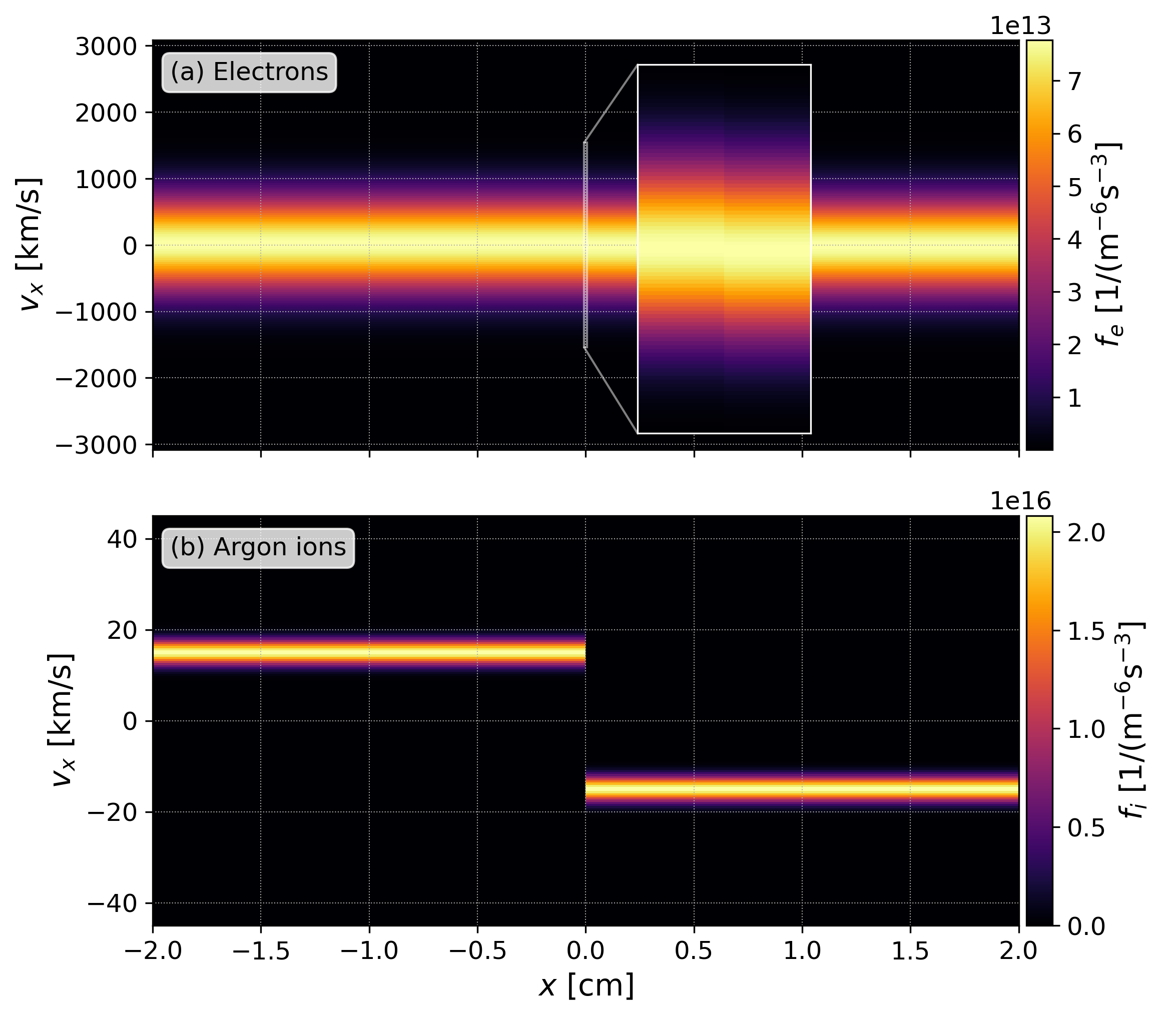
Figure 1: Initial conditions of the electron and ion distribution function for two $15\text{\,}\mathrm{k}\mathrm{m}\mathrm{/}\mathrm{s}$ argon jets over the whole $4\text{\,}\mathrm{c}\mathrm{m}$ domain. The initial temperature is set to $1.5\text{\,}\mathrm{e}\mathrm{V}$ for both species. As the thermal velocity of electrons is, at this temperature, high relative to the jet velocity, the initial discontinuity in the electron distribution function is barely noticeable even within the expanded scale presented.

III.1 Effectiveness of the PKPM model

To demonstrate the effectiveness of the hybrid PKPM model, we run three simulations from the same initial conditions in computational domains with one (1V) and three (3V) velocity dimensions. Figure 2 shows the three ion distribution functions after $0.1\text{\,}\mathrm{\SIUnitSymbolMicro}\mathrm{s}$ from the initial contact. All these cases use the same collisional model, the only differences are the number of velocity dimensions and the extra perpendicular equations in the PKPM model. Note that the velocity resolution is slightly reduced in comparison to Fig. 1 to make this test less computationally expensive. Panel (a) shows the 1V model, panel (b) the PKPM model, and panel (c) the 3V model. The full 3V distribution function in the latter case has been integrated over the $v_{y}$ and $v_{z}$ directions for comparison. Figure 2 shows the remarkable accuracy of the PKPM model as compared to the full 3V simulation.

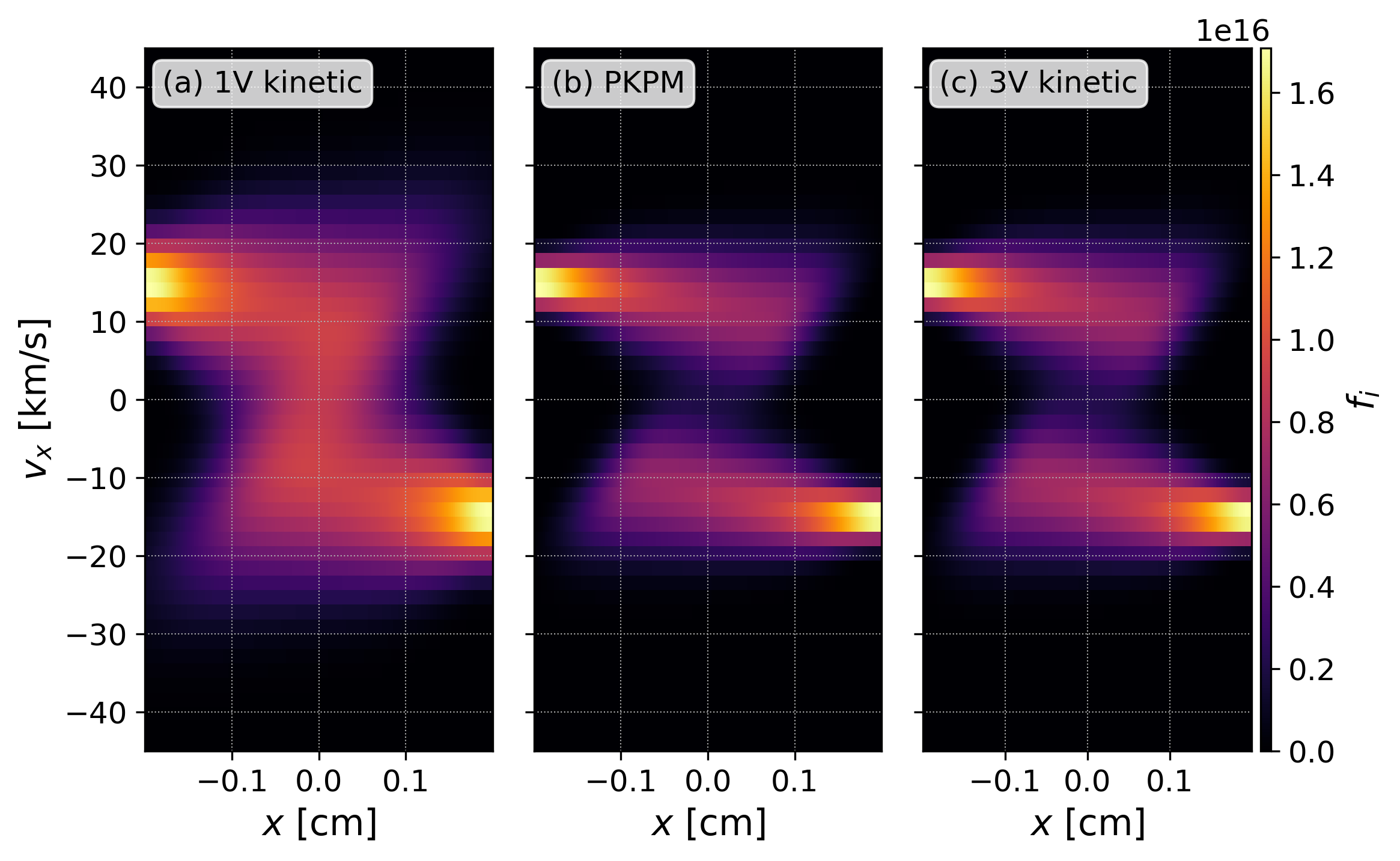
Figure 2: Comparison of simulations with one velocity dimension (1V), hybrid simulation with kinetic description in the $x$-direction coupled with parallel temperature evolution (PKPM), and with full three-dimensional velocity space (3V). The full 3V distribution function has been integrated over the $v_{y}$ and $v_{z}$ directions for comparison. All three cases are evolved for $0.1\text{\,}\mathrm{\SIUnitSymbolMicro}\mathrm{s}$ from the initial contact. Note that the PKPM and 3V solutions are in agreement and they differ from the 1V solution.

Figure 3 supplements the distribution functions from Fig. 2 with integrated moments; number density, flux, and temperature. The PKPM and 3V models agree well for density and flux. Even though the electron temperature is underestimated in the PKPM model, it is still more accurate than in the 1V model. Finally, ion parallel temperatures match while the heat transfer to the perpendicular direction lags in the PKPM model in comparison to 3V.

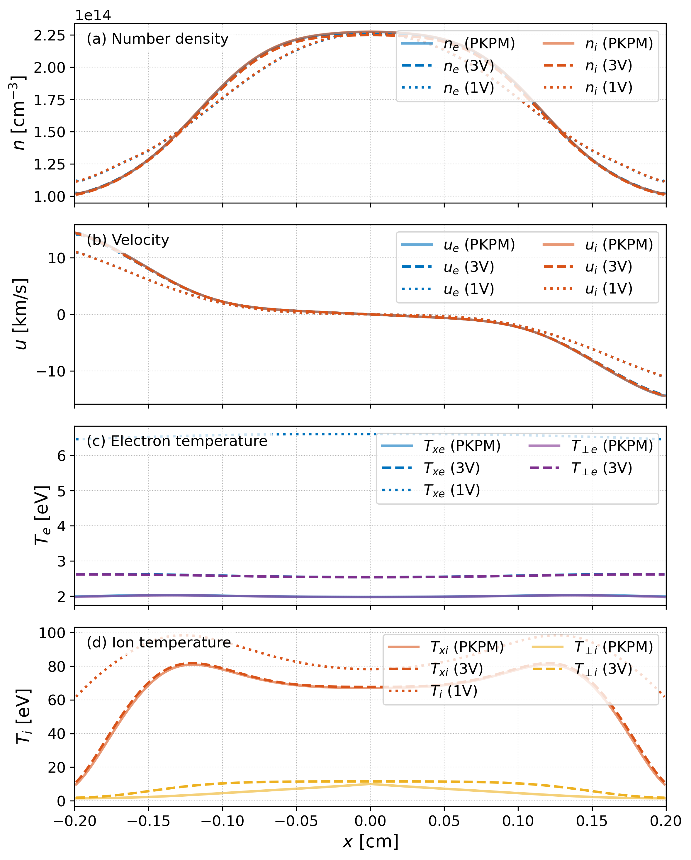
Figure 3: Moments of the distribution functions in Fig. 2; (a) number density, (b) particle flux, (c) electron temperatures, and (d) ion temperatures. The goal is to establish how the hybrid PKPM model agrees with the 3V model relative to the 1V model. Densities, fluxes, and parallel ion temperatures show a good agreement. The electron temperatures are underestimated but have better agreement than the 1V model, and ion thermalization in the perpendicular dimension lags behind the 3V model. Note that in this case, the parallel and perpendicular electron profiles are on top of each other due to high electron-electron collision frequency.

This gives us confidence that PKPM can successfully replicate 3V simulations for these cases. The PKPM model provides access to computationally-efficient fully explicit kinetic simulations on a domain spanning several centimeters while resolving the collisional mean-free-path for a couple of $\mu\mathrm{s}$. Simulations using the PKPM model take just a few hours on a single GPU. The computational cost is only marginally higher than for a 1V simulation. These comparisons demonstrate that the 1V model produces substantially different results and is not accurate for these problems.

III.2 Collision of cold beams

In the $15\text{\,}\mathrm{k}\mathrm{m}\mathrm{/}\mathrm{s}$ case (Fig. 1), both species collide to form a Maxwellian distribution with zero bulk velocity. The higher collision frequency of electrons results in a small variance from the Maxwellian distribution across the whole simulation domain while the heavier argon ions form non-Maxwellian transition regions (approximately between 0.5 and $0.75\text{\,}\mathrm{c}\mathrm{m}$ in Fig. 4b). Note that the trapping potential (i.e., the velocity $v_{x}$ for which $1/2mv_{x}^{2}=|q\phi|$), represented by the green line in Fig. 4a encompasses a trapping region. In the case of collisionless electrostatic shocks, electrons typically fill the trapping region forming a “flat-top” distribution.[24, 25, 26] Here, electrons retain the Maxwellian velocity distribution while expanding beyond the trapping region due to their high collision frequency.

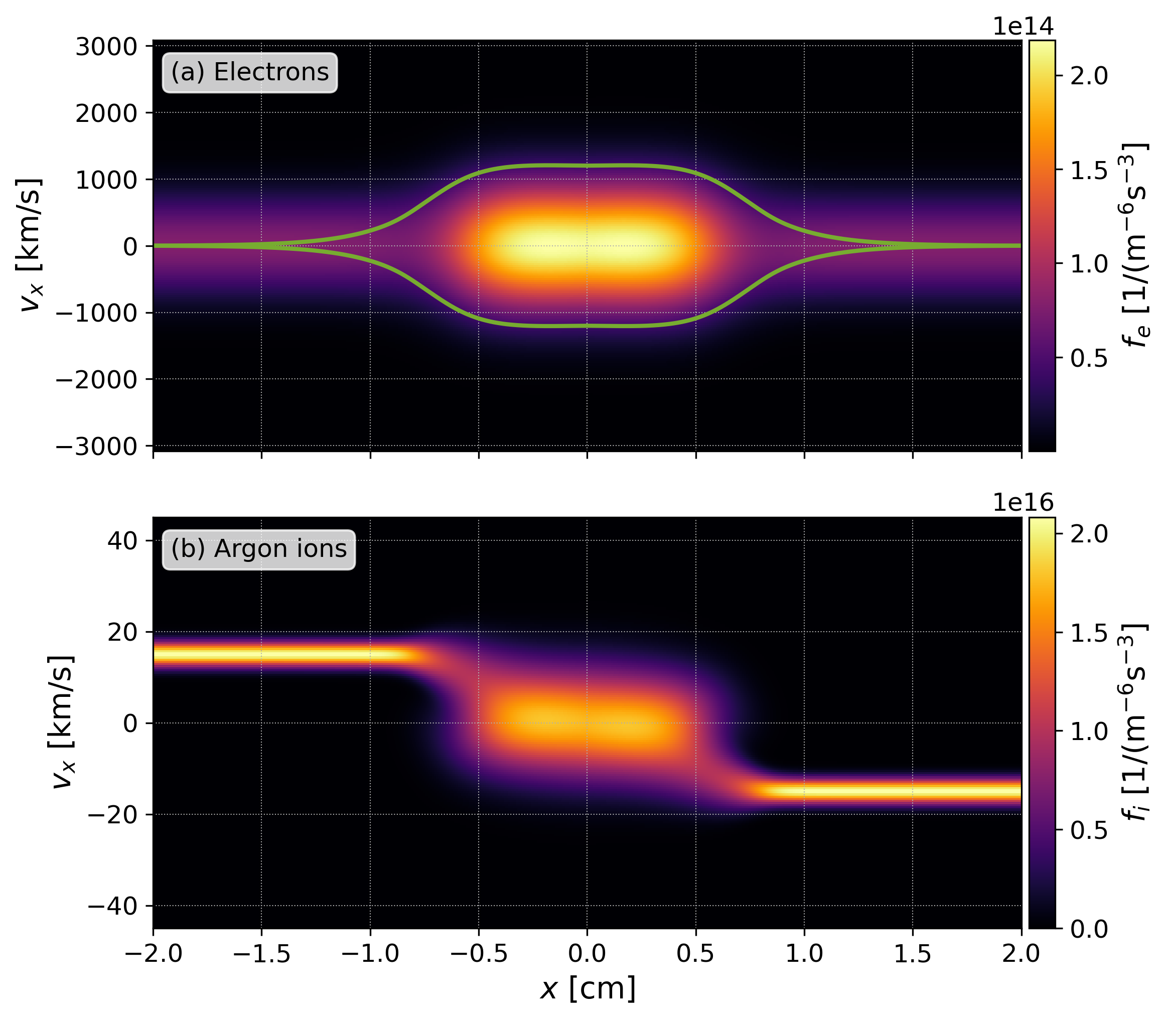
Figure 4: Electron and ion distribution functions, evolved for $1\text{\,}\mathrm{\SIUnitSymbolMicro}\mathrm{s}$ from the initial conditions shown in Fig. 1 (the point of contact). The ion populations collide, forming a Maxwellian distribution with zero bulk velocity and increased density. Additionally, the green line in the electron plot corresponds to the trapping potential, i.e., the velocity $v_{x}$ for which $1/2mv_{x}^{2}=|q\phi|$. Note that the potential is calculated during postprocessing and the simulation uses Vlasov-Maxwell model.

This simulation uses the Spitzer formula to calculate the collision frequency in Eq. (3). As we will show later in Fig. 10, these results are in agreement with experimental measurements. However, this was not the case for the faster, $50\text{\,}\mathrm{k}\mathrm{m}\mathrm{/}\mathrm{s}$ $1.5\text{\,}\mathrm{e}\mathrm{V}$ jets. There the same simulation approach still results in a merge while the experimental results show interpenetration. This is due to the fact that the reduced collisional model assumes a collisional frequency independent of velocity and overestimates the effect of collisions for tails of the distribution function. Note that in the case of the faster jets, the thermal velocity is significantly lower than the bulk velocity ($v_{th}=$1.9\text{\,}\mathrm{k}\mathrm{m}\mathrm{/}\mathrm{s}$$).

To capture the collisions between two cold beams, the full Fokker-Planck operator[27] is required;

$$-\frac{1}{2}\nabla_{v}\cdot\big{(}\bm{a}f-\bm{D}\cdot\nabla_{v}f\big{)},$$ (16)

where $\bm{a}$ and $\bm{D}$ are calculated from the Rosenbluth potentials, $h(\bm{x},\bm{v})$ and $g(\bm{x},\bm{v})$.

We can get a better understanding of the interaction between the beams, by approximating an effective collision frequency from the initial conditions. $\bm{a}$ in Eq. (16) is defined as

$$\frac{1}{2}\bm{a}=\Gamma\nabla_{v}h(\bm{x},\bm{v}),$$ (17)

where $\Gamma=4\pi\Lambda(Ze)^{4}/m^{2}$ ($Z$ is assumed 1 here) and $\Lambda$ is the Coulomb logarithm. Since $h$ is defined as $\nabla^{2}h=-f$, it can be calculated analytically for the Maxwellian distribution $f$. Without loss of generality, we can assume a zero bulk velocity to get,

$$h_{M}(\bm{x},\bm{v})=\frac{n(\bm{x})}{v}\mathrm{erf}\left(\frac{v}{\sqrt{2}v_{th}(\bm{x})}\right),$$ (18)

where $v=\sqrt{v_{x}^{2}+v_{y}^{2}+v_{z}^{2}}$. Taking the velocity gradient from Eq. (17) leads to

$$\nabla_{v}h_{M}(\bm{x},\bm{v})=\left[\frac{\sqrt{2}}{\sqrt{\pi}}\frac{n}{v_{th}}\frac{\exp\left(-\frac{v^{2}}{2v_{th}^{2}}\right)}{v^{2}}-n\frac{\mathrm{erf}\left(\frac{v}{\sqrt{2}v_{th}}\right)}{v^{3}}\right].$$ (19)

Comparing the forms of Eq. (3) and Eq. (16) leads to the effective collision frequency,

$$\nu_{ef}(\bm{v})=-\Gamma\left[\frac{\sqrt{2}}{\sqrt{\pi}}\frac{n}{v_{th}}\frac{\exp\left(-\frac{v^{2}}{2v_{th}^{2}}\right)}{v^{2}}-n\frac{\mathrm{erf}\left(\frac{v}{\sqrt{2}v_{th}}\right)}{v^{3}}\right].$$ (20)

$\nu_{ef}(\bm{v})$ is the effective collision frequency between a test particle at $\bm{v}$ and a non-drifting Maxwellian with number density $n$ and thermal velocity $v_{th}$. Since the goal of this approximation is to estimate the effect of collisions between the two jets, i.e., the collision frequency between a particle in one jet and particles in the other jet, we can set $|\bm{v}|=\Delta u=2u$ (internally, the jets are collisional).

Interestingly, Eq. (20) gives comparable results to the Spitzer formula of the collision frequency for the slower jets ($15\text{\,}\mathrm{k}\mathrm{m}\mathrm{/}\mathrm{s}$). However, the collision frequency decreases approximately by an order of magnitude for the faster jets ($50\text{\,}\mathrm{k}\mathrm{m}\mathrm{/}\mathrm{s}$) where the Spitzer formula would not apply.

Eq. (20) assumes a Maxwellian distribution of particles and is only valid before the jets start to merge. Therefore, the full FPO is required to study the details of the shock-forming process. Still, calculating the effective collision frequency, $\nu_{eff}$, and using it in Eq. (3) is sufficient to answer the question of whether the jets are going to form a shock or just interpenetrate for a range of parameter scans across density, temperature, and velocities. Therefore, it can be used to quickly guide an experimental setup and perform broad parameter studies. $\nu_{eff}$ is used exclusively in the rest of this work. In follow-up work, we will complement this approximation with the full FPO simulations of selected cases.

IV Scaling study

Using the frequency Eq. (20), we can set up a wide variety of relatively fast numerical simulations. Upon merging, the variations in the temperature, density, and bulk velocity ($|\bm{v}|=\Delta u=2u$) result in either an interpenetration of the jets or an increase in the density. Figure 5 shows a 3D sample of a parameter space where the effective collision frequency is color-coded. This illustrates that the collision frequency drops by over an order of magnitude between the 15 and $50\text{\,}\mathrm{k}\mathrm{m}\mathrm{/}\mathrm{s}$ jets.

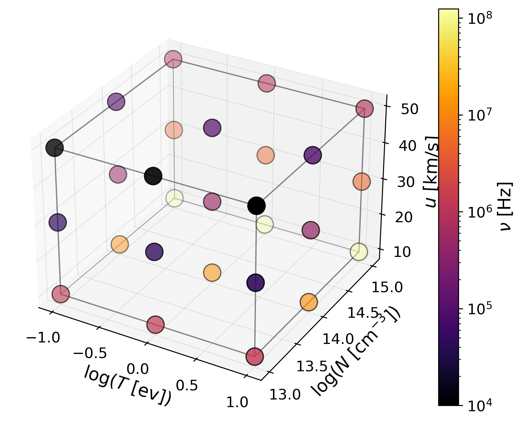
Figure 5: Effective collision frequencies from Eq. (20) calculated for the initial parameter space defined by temperature, density, and jet bulk velocity. Note that the scales of the density, temperature, and collision frequency are logarithmic.

A particular feature of Fig. 5 is the independence of the effective collision frequency on the temperature (for these jet velocities). This is consistent with the low thermal velocity relative to the bulk velocity, i.e., the argon ions behave like cold beams. Figure 6 shows the dependence of the collision frequency from Eq. (20) on the relative velocity (for symmetric jets $\Delta u=2u$). The three studied temperatures (0.1, 1, and $10\text{\,}\mathrm{e}\mathrm{V}$) give identical results for relative velocities higher than $20\text{\,}\mathrm{k}\mathrm{m}\mathrm{/}\mathrm{s}$. The lower two temperatures effectively match across the whole range of relative velocities.

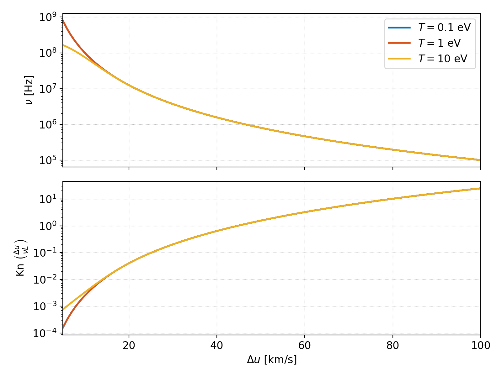
Figure 6: Ion-ion collision frequencies (top panel) from Eq. (20) for density of $1\text{\times}{10}^{14}\text{\,}\mathrm{c}\mathrm{m}^{-3}$ and three temperatures, 0.1, 1, and $10\text{\,}\mathrm{e}\mathrm{V}$ based on the relative velocity (for symmetric jets $\Delta u=2u$). All three temperatures give identical results for relative velocities higher than $20\text{\,}\mathrm{k}\mathrm{m}\mathrm{/}\mathrm{s}$.Bottom panel shows corresponding Knudsen number where the mean free path is calculated as $\Delta u/\nu$ and $L$ is taken as the simulation domain size of $4\text{\,}\mathrm{c}\mathrm{m}$.

With the temperature having a negligible impact on the collision frequency in the regimes considered, several additional simulations for different jet velocities are performed to help find the transition point between interpenetration and shock formation. Figure 7 and Fig. 8 show two initial densities, $1\text{\times}{10}^{13}\text{\,}\mathrm{c}\mathrm{m}^{-3}$ and $1\text{\times}{10}^{14}\text{\,}\mathrm{c}\mathrm{m}^{-3}$ for the temperature of $1\text{\,}\mathrm{e}\mathrm{V}$.

Figure 7 captures the number densities at $0.5\text{\,}\mathrm{\SIUnitSymbolMicro}\mathrm{s}$ after the contact. Note that in a fluid simulation with Euler equations, the density would quickly jump by a factor of four and form sharp gradients; however, this is not the case here due to the finite collision frequency. The lower density, Fig. 7a, results in lower collision frequency and the jets mostly interpenetrate. Only the lower jet velocities have density accumulation in the middle, where the density goes above the superposition of the two jets. This density is going to increase for as long as there is a flow of plasma but the feature is going to be diffused. In the case of the higher density, Fig. 7b, there is a transition velocity below which there is significant accumulation in the center and sharp features arise. Similar to the lower density case, the number density will increase for as long as the source of plasma is present. As it was mentioned above, the goal of this method is to capture the transition between the shock and interpenetrating regime, not to study subsequent details of the shock formation. Therefore, the results for cases where density significantly increases should be seen as qualitative.

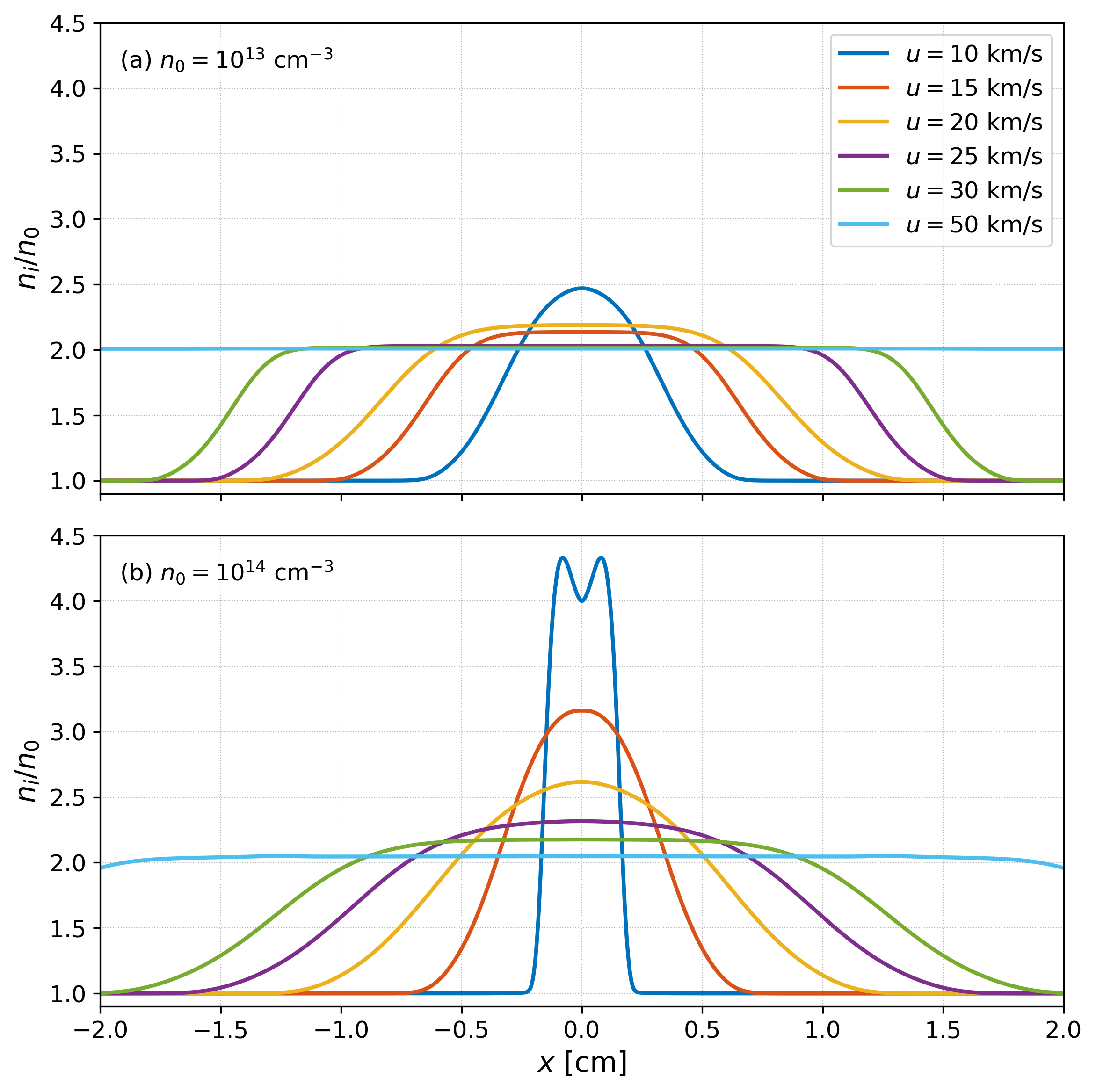
Figure 7: Comparison of densities for several jet velocities after $0.5\text{\,}\mathrm{\SIUnitSymbolMicro}\mathrm{s}$. Two initial densities, $1\text{\times}{10}^{13}\text{\,}\mathrm{c}\mathrm{m}^{-3}$ and $1\text{\times}{10}^{14}\text{\,}\mathrm{c}\mathrm{m}^{-3}$, are shown. Only lower velocities for the lower density case are merging while the higher velocity jets are simply streaming through each other.

In addition to densities in Fig. 7, Fig. 8 provides line-outs of the ion distribution function in the middle of the domain. The line colors are consistent with those in Fig. 7. The top panel shows that the only case with density growth (the $10\text{\,}\mathrm{k}\mathrm{m}\mathrm{/}\mathrm{s}$ case) is also the only one where the ion jets are merging. The jets remain distinctly separate in all the other cases. The distribution functions in the higher density case are clearly merging to form a central shocked region for most of the jet velocities considered.

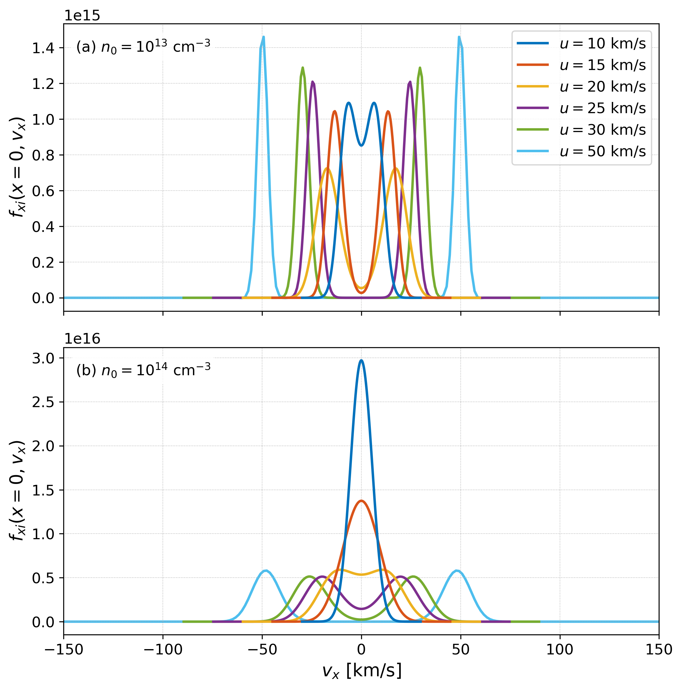
Figure 8: Comparison of distribution function lineouts at $x=0$ for several jet velocities after $0.5\text{\,}\mathrm{\SIUnitSymbolMicro}\mathrm{s}$. Two initial densities, $1\text{\times}{10}^{13}\text{\,}\mathrm{c}\mathrm{m}^{-3}$ (top) and $1\text{\times}{10}^{14}\text{\,}\mathrm{c}\mathrm{m}^{-3}$ (bottom), are shown. These plots show a clear difference between the cases where jets merge and where the jets interpenetrate. Note that for the lower density, the collision frequency is lower and even the slowest tested jet does not fully merge in time, still presenting double peaks. In the higher-density case, the two slowest cases are fully merged.

V Comparison to experimental data

The simulations in the previous section demonstrate the potential of the hybrid model with a reduced number of fully resolved velocity dimensions to predict different jet-merging regimes. In order to validate our results, we look at the preliminary PLX data from shots with two jets with normal incidence, which are the closest to the simulation setup. The experimental chamber is cylindrical, $76\text{\,}\mathrm{c}\mathrm{m}$ in diameter and $130\text{\,}\mathrm{c}\mathrm{m}$ long, and uses plasma guns from PLX to recreate similar conditions, but is itself separate from the PLX chamber. Figure 9 shows a diagram of this chamber along with the spectral line of sight from which Doppler shift measurements are obtained. At each end is mounted one of the plasma guns which launch the jets. Gas feed pressure and discharge voltage of the guns can be adjusted to vary the jet speed and explore the breaking point between merging and interpenetrating jets. Figure 10 shows intensity data from the Doppler shift measurements, where the wavelength has been converted to velocity. The spectral line of sight is 45 degrees with respect to the jet axis, which is accounted for in converting from Doppler wavelength shift to the axial ion velocity distribution in the figure. There we clearly see the slower jets merging (top) and faster jets retaining two peaks (bottom); they do not merge even later in time. Note that the times in this figure are measured from the shot and not from the point of contact as is the case for the simulation results. The intensity asymmetry of the distribution functions is most likely caused by the line-of-sight of the diagnostics being under an angle with respect to the jets, with the farther jet contributing a lesser overall intensity.

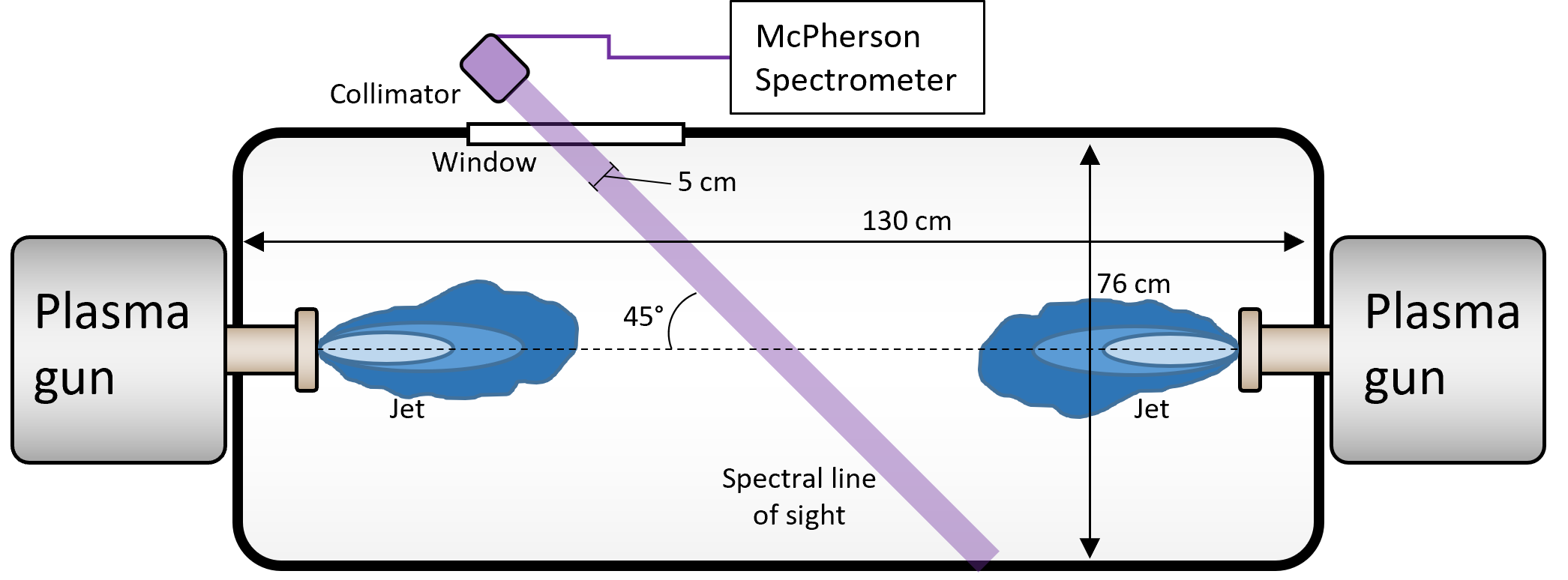
Figure 9: A diagram of the experimental of the jet merging chamber that uses plasma guns from PLX. The purple highlighted region indicates the spectral line of sight approximately $5\text{\,}\mathrm{c}\mathrm{m}$ wide through which the Doppler shift measurements are acquired.

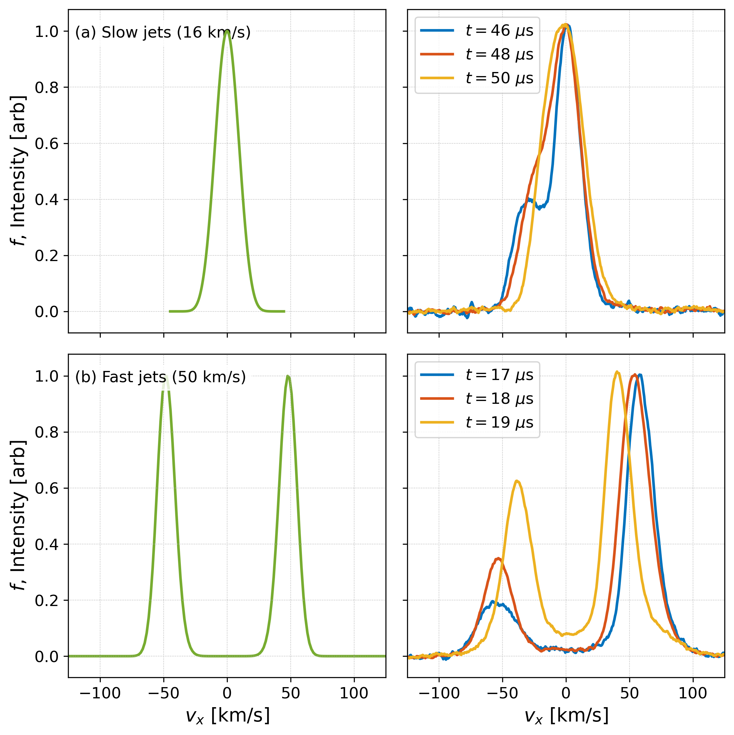
Figure 10: Doppler shift measurements of the ArII $434.8\text{\,}\mathrm{n}\mathrm{m}$ emission from PLX (right column) which directly correlate to the simulation distribution function as seen in the left column and Fig. 8(b).

These results agree with the model predictions where the slow jets merge while the faster jets interpenetrate. The time in this figure is measured from the shot and not from the point of contact as is the case for the simulation results.

VI Closing remarks and Summary

It is important to note that when these cases are simulated using a five-moment two-fluid model,[28, 29, 30] the merging of the jets will always produce a shock with sharp density gradients. Figure 11 shows the three cases with higher density from Fig. 7b along with results from the five-moment two-fluid model implemented in Gkeyll. While the position of the gradients does match for the slowest case, where the collision frequency is relatively high, the other cases produce very different results. As a result, fluid models cannot be used to accurately predict shocked versus shock-mitigated (or interpenetrating) jet merging.

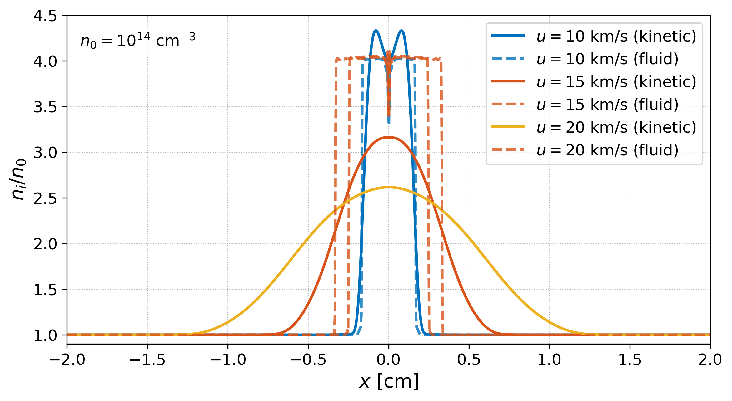
Figure 11: The exact density profile as seen in Fig. 7 with an addition of densities from the Gkeyll five-moment fluid model. Note that even if the fluid model is started with exactly the same parameters, it would always result in a shock and sharp gradient. The kinetic results with finite collision frequency are significantly more diffused.

To summarize, the transition between collisional and collisionless jet merging is vital to understand in a variety of plasma systems. To accurately model these phenomena one requires not only a kinetic method but a kinetic method that accurately describes all of the degrees of freedom of the plasma. We have demonstrated such a model with our novel parallel-kinetic-perpendicular-moments model that decomposes the collisionless dynamics parallel and perpendicular to the jet merging process. We find that slow jets merge and shock while faster jets are sufficiently collisionless to simply interpenetrate. These results are in agreement with PLX measurements.

We emphasize that the kinetic model presented in this paper is unique not only in its capability of simulating the transition between collisional and collisionless jets, but in the quality of the distribution function data the method produces from the grid-based approach employed. Thus, the grid-based method employed here not only contains the key kinetic physics required to model these systems but also eliminates the counting noise typical of other numerical approaches such as the particle-in-cell method which can be problematic for analysis of the distribution function and overall solution quality.[31] We anticipate this approach to be of high utility for future jet merging studies which include geometric effects such as the angle of jet merging.

VII Getting Gkeyll and reproducing the results

To allow interested readers to reproduce our results, full installation instructions for Gkeyll are provided on the Gkeyll website (http://gkeyll.readthedocs.io). The code can be installed on Unix-like operating systems (including Mac OS and Windows using the Windows Subsystem for Linux) by building the code via sources. Input files for the simulations presented here are available in the following GitHub repository, https://github.com/ammarhakim/gkyl-paper-inp.

VIII Acknowledgment

This work was supported by the Department of Energy ARPA-E BETHE program under award number DE-AR0001263.

The authors acknowledge Advanced Research Computing at Virginia Tech for providing computational resources and technical support that have contributed to the results reported in this paper. URL: https://arc.vt.edu

References

- Biskamp [1973] D. Biskamp, “Collisionless shock waves in plasmas,” Nuclear Fusion 13, 719 (1973).
- Liberman, Velikovich, and Dobroslavski [1986] M. A. Liberman, A. L. Velikovich, and A. Dobroslavski, Physics of shock waves in gases and plasmas (Springer, 1986).
- Casanova, Larroche, and Matte [1991] M. Casanova, O. Larroche, and J.-P. Matte, “Kinetic simulation of a collisional shock wave in a plasma,” Physical review letters 67, 2143 (1991).
- Thio et al. [1999] Y. Thio, E. Panarella, R. Kirkpatrick, C. Knapp, F. Wysocki, P. Parks, and G. Schmidt, “Magnetized target fusion in a spheroidal geometry with standoff drivers,” in Current Trends in International Fusion Research: Proceedings of the Second Symposium (Ottawa, ON, Canada: Nat. Res. Council Canada, 1999) pp. 113–134.
- Hsu et al. [2012] S. C. Hsu, T. Awe, S. Brockington, A. Case, J. Cassibry, G. Kagan, S. Messer, M. Stanic, X. Tang, D. Welch, et al., “Spherically imploding plasma liners as a standoff driver for magnetoinertial fusion,” Ieee transactions on plasma science 40, 1287–1298 (2012).
- Knapp and Kirkpatrick [2014] C. E. Knapp and R. Kirkpatrick, “Possible energy gain for a plasma-liner-driven magneto-inertial fusion concept,” Physics of Plasmas 21, 070701 (2014).
- Gregory et al. [2009] C. Gregory, J. Howe, B. Loupias, S. Myers, M. Notley, Y. Sakawa, A. Oya, R. Kodama, M. Koenig, E. Falize, et al., “Colliding plasma experiments to study astrophysical-jet relevant physics,” Astrophysics and space science 322, 37–41 (2009).
- Ryutov et al. [2012] D. Ryutov, N. Kugland, H.-S. Park, C. Plechaty, B. Remington, and J. Ross, “Intra-jet shocks in two counter-streaming, weakly collisional plasma jets,” Physics of Plasmas 19, 074501 (2012).
- Mohammed and Adams [2022] A. Mohammed and C. Adams, “Ion shock layer formation during multi-ion-species plasma jet stagnation events,” Physics of Plasmas 29, 072307 (2022).
- Falk [2018] K. Falk, “Experimental methods for warm dense matter research,” High Power Laser Science and Engineering 6 (2018).
- Case et al. [2013] A. Case, S. Messer, S. Brockington, L. Wu, F. D. Witherspoon, and R. Elton, “Merging of high speed argon plasma jets,” Physics of Plasmas 20, 012704 (2013).
- Merritt et al. [2014] E. C. Merritt, A. L. Moser, S. C. Hsu, C. S. Adams, J. P. Dunn, A. Miguel Holgado, and M. A. Gilmore, “Experimental evidence for collisional shock formation via two obliquely merging supersonic plasma jets,” Physics of Plasmas 21, 055703 (2014).
- Hsu et al. [2015] S. Hsu, A. Moser, E. Merritt, C. Adams, J. Dunn, S. Brockington, A. Case, M. Gilmore, A. Lynn, S. Messer, et al., “Laboratory plasma physics experiments using merging supersonic plasma jets,” Journal of Plasma Physics 81 (2015).
- Hsu et al. [2017] S. Hsu, S. Langendorf, K. Yates, J. Dunn, S. Brockington, A. Case, E. Cruz, F. Witherspoon, M. Gilmore, J. Cassibry, et al., “Experiment to form and characterize a section of a spherically imploding plasma liner,” IEEE Transactions on Plasma Science 46, 1951–1961 (2017).
- Juno et al. [2018] J. Juno, A. Hakim, J. TenBarge, E. Shi, and W. Dorland, “Discontinuous Galerkin algorithms for fully kinetic plasmas,” Journal of Computational Physics 353, 110–147 (2018).
- Hakim et al. [2020] A. Hakim, M. Francisquez, J. Juno, and G. W. Hammett, “Conservative discontinuous Galerkin schemes for nonlinear Dougherty–Fokker–Planck collision operators,” Journal of Plasma Physics 86 (2020).
- Hakim and Juno [2020] A. Hakim and J. Juno, “Alias-free, matrix-free, and quadrature-free discontinuous Galerkin algorithms for (plasma) kinetic equations,” in SC20: International Conference for High Performance Computing, Networking, Storage and Analysis (IEEE, 2020) pp. 1–15.
- Francisquez et al. [2022] M. Francisquez, J. Juno, A. Hakim, G. W. Hammett, and D. R. Ernst, “Improved multispecies Dougherty collisions,” Journal of Plasma Physics 88 (2022).
- Cockburn and Shu [1998] B. Cockburn and C.-W. Shu, “The Runge–Kutta discontinuous Galerkin method for conservation laws v: multidimensional systems,” Journal of Computational Physics 141, 199–224 (1998).
- Cockburn and Shu [2001] B. Cockburn and C.-W. Shu, “Runge–Kutta discontinuous Galerkin methods for convection-dominated problems,” Journal of scientific computing 16, 173–261 (2001).
- Hesthaven and Warburton [2007] J. S. Hesthaven and T. Warburton, Nodal discontinuous Galerkin methods: algorithms, analysis, and applications (Springer Science & Business Media, 2007).
- Arnold and Awanou [2011] D. N. Arnold and G. Awanou, “The serendipity family of finite elements,” Foundations of computational mathematics 11, 337–344 (2011).
- Cagas et al. [2017] P. Cagas, A. Hakim, J. Juno, and B. Srinivasan, “Continuum kinetic and multi-fluid simulations of classical sheaths,” Physics of Plasmas 24, 022118 (2017).
- Forslund and Shonk [1970] D. Forslund and C. Shonk, “Formation and structure of electrostatic collisionless shocks,” Physical Review Letters 25, 1699 (1970).
- Pusztai et al. [2018] I. Pusztai, J. M. TenBarge, A. N. Csapó, J. Juno, A. Hakim, L. Yi, and T. Fülöp, “Low Mach-number collisionless electrostatic shocks and associated ion acceleration,” Plasma Physics and Controlled Fusion 60, 035004 (2018).
- Sundström et al. [2019] A. Sundström, J. Juno, J. M. TenBarge, and I. Pusztai, “Effect of a weak ion collisionality on the dynamics of kinetic electrostatic shocks,” Journal of Plasma Physics 85 (2019).
- Rosenbluth, MacDonald, and Judd [1957] M. Rosenbluth, W. MacDonald, and D. Judd, “Fokker-Planck equation for an inverse-square force,” Physical Review 107, 1 (1957).
- Hakim, Loverich, and Shumlak [2006] A. Hakim, J. Loverich, and U. Shumlak, “A high resolution wave propagation scheme for ideal two-fluid plasma equations,” Journal of Computational Physics 219, 418–442 (2006).
- Srinivasan and Shumlak [2011] B. Srinivasan and U. Shumlak, “Analytical and computational study of the ideal full two-fluid plasma model and asymptotic approximations for Hall-magnetohydrodynamics,” Physics of Plasmas 18, 092113 (2011).
- Shumlak et al. [2011] U. Shumlak, R. Lilly, N. Reddell, E. Sousa, and B. Srinivasan, “Advanced physics calculations using a multi-fluid plasma model,” Computer Physics Communications 182, 1767–1770 (2011).
- Juno et al. [2020] J. Juno, M. Swisdak, J. Tenbarge, V. Skoutnev, and A. Hakim, “Noise-induced magnetic field saturation in kinetic simulations,” Journal of Plasma Physics 86, 175860401 (2020).