Deep learning of spatial densities in inhomogeneous correlated quantum systems

Abstract

Machine learning has made important headway in helping to improve the treatment of quantum many-body systems. A domain of particular relevance are correlated inhomogeneous systems. What has been missing so far is a general, scalable deep-learning approach that would enable the rapid prediction of spatial densities for strongly correlated systems in arbitrary potentials. In this work, we present a straightforward scheme, where we learn to predict densities using convolutional neural networks trained on random potentials. While we demonstrate this approach in 1D and 2D lattice models using data from numerical techniques like Quantum Monte Carlo, it is directly applicable as well to training data obtained from experimental quantum simulators. We train networks that can predict the densities of multiple observables simultaneously and that can predict for a whole class of many-body lattice models, for arbitrary system sizes. We show that our approach can handle well the interplay of interference and interactions and the behaviour of models with phase transitions in inhomogeneous situations, and we also illustrate the ability to solve inverse problems, finding a potential for a desired density.

Predicting the properties of quantum many-body systems is one of the most important challenges in physics, as it is relevant for quantum chemistry and materials science, as well as for more recent tasks like benchmarking quantum simulators. This is a hard problem for larger system sizes, due to the exponential explosion of the Hilbert space dimension. Elaborate approximation schemes have been developed, including various forms of perturbation theory, mean-field approaches like density-functional theory (DFT), cluster methods, Monte Carlo methods, and several variational-ansatz ideas, including tensor network constructions. Machine learning has entered this field of predicting quantum matter some years ago, with results that show great promise, turning it into an important tool  Carrasquilla (2020); Carleo et al. (2019); Dawid et al. (2022). It has led to improvements in several directions, like the use of neural networks to represent variational wave functions Carleo and Troyer (2017); Schmitt and Heyl (2020); Hartmann and Carleo (2019), to improve DFT calculations  Brockherde et al. (2017); Costa et al. (2022); Chandrasekaran et al. (2019); Ryczko et al. (2019); Nelson et al. (2019); Moreno et al. (2019), as well as in molecular dynamics Behler and Parrinello (2007); Bartók et al. (2017).

However, the range of validity of such schemes is often limited, making it necessary to carefully select the approach depending on circumstances. Furthermore, the effort expended in applying the techniques to larger-scale inhomogeneous systems can still be quite substantial. It would, therefore, be desirable to employ machine learning to circumvent entirely these tailored approaches and arrive at a more general method for rapidly predicting the properties of quantum many-body systems. This is especially true in inhomogeneous situations where the need for a scalable approach that can treat large sizes in extended systems arises.

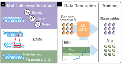
Figure 1: Overview of the approach. (a) The convolutional neural network maps a potential landscape of arbitrary size, together with model parameters, to the spatial maps of multiple observables (including correlators, here denoted as ’noise’). (b) Training procedure. Any of a set of numerical methods are used to turn random potentials into spatial maps, providing the training data. The dependence of energy on particle number is recorded as well and gives access to the chemical potential.

Here we introduce a straightforward scheme to train a deep convolutional network that is able to directly predict spatial properties of many-body ground states or thermal states in arbitrary potential landscapes. The key idea is to train on random, spatially non-uniform potentials and for variable particle numbers, where the corresponding predictions can be extracted from any numerical method or potentially even from experimental data. In general, the network is designed with a multi-headed structure and can thus be trained to produce the spatial maps of several physical observables simultaneously. This is intended to make it more sample-efficient in training, sharing one initial processing block among observables (see Fig 1a for a schematic).

In addition, we introduce the capability of training a single network on a range of model parameters, such as coupling values and interaction strengths. This again is designed to boost sample efficiency, since one network is trained on data pertaining to the full parameter range, giving it the potential to make predictions that are partially informed by behaviour seen at other parameter values.

Even though the generation of training data may be computationally expensive and may require a large-scale computing cluster, once the network has been trained our method allows rapid exploration of inhomogeneous quantum many-body systems with low computational effort on single processors; examples show that for typical parameters speedups of a factor of a million are realistic. Due to the local nature of the convolution, the network can be exploited to make reliable predictions for inhomogeneous systems far larger than those it has been trained on previously, provided that training sample sizes and the combined range of the stacked convolutions exceed the physical correlation length. One potential application of the trained network would be Hamiltonian learning Valenti et al. (2019), finding underlying parameters and potentials given experimentally observed densities via gradient descent. Another application would be the inverse design of potentials with desired characteristics, either via exploiting the rapid predictions in gradient-free methods or implementing direct gradient descent.

In previous works, scalable approaches based on convolutional or recurrent neural networks have been proposed in the context of quantum many-body systems. Those approaches map a potential to a scalar global variable like the energy Saraceni et al. (2020); Mujal et al. (2021) or to level-spacing statistics Gresch et al. (2022). In contrast, our approach maps a potential to several spatial distributions of observables like the density. Although there have also been some works that investigate the direct prediction of densities, those were in the context of small few-particle quantum-chemistry type scenarios Ryczko et al. (2019), where scalability and application to an extensive system was not an issue.

We consider interacting lattice models of fermions or bosons, subject to a potential landscape $V(x)$, where $x$ denotes the discrete lattice location. Our aim is to train a deep neural network to be able to predict the spatial dependence of the ground-state expectation values of interesting observables when it is provided with the potential. These observables may include the density ${\hat{n}}(x)={\hat{a}}^{\dagger}(x){\hat{a}}(x)$, the coherences that enter the density matrix ${\hat{a}}^{\dagger}(x+\delta x){\hat{a}}(x)$ (which can be used to express the current flow if $x+\delta x$ denotes a neighboring site), or fluctuations like ${\hat{n}}(x+\delta x){\hat{n}}(x)$.

In our approach, the starting point for training is the evaluation of such spatial observable maps by any of a number of numerical techniques, like exact diagonalization (ED) or quantum Monte Carlo (QMC). Training samples are produced by generating random potentials and calculating predictions for those. We take these potentials to be realizations of both white and colored noise, with similar results. Samples are produced on relatively small finite-size systems of linear extent $L$, and for different choices of particle number $N$.

This idea is related to a recent approach trying to learn the dynamics of quantum many-body systems by observing their behaviour under random temporal driving Mohseni et al. (2022).

One important characteristic of our approach is that we are interested in using the network to produce predictions for arbitrary-size systems later on. In order to handle that, we choose to work in the grand-canonical ensemble, where the particle number can be tuned via the chemical potential $\mu$. Instead of taking $V(x),N,L$ as input, we hence feed $V(x)-\mu$ into the network. To facilitate this, during the sample generation phase we scan the evolution of ground-state energy $E$ vs. particle number $N$ and extract $\mu$ from the resulting dependency. Specifically, for each sample fed into the network, given $E(N)$ we pick $\mu$ drawn uniformly from the interval $\left[E(N)-E(N-1),E(N+1)-E(N)\right]$. This ansatz effectively produces an interpolated version of $\mu(N)$ and leads to the desired ability to scale to arbitrary sizes $L$. For the specific QMC method we use in our studies, $\mu$ can be prescribed directly (see Fig. 1b for a summary of the described procedure).

One central aim in selecting the architecture of our network is to make sure to maximize the sample efficiency, i.e. to exploit as much as possible the information contained in the training data, which is expensive to generate. In general, the architecture of the convolutional network is set up with a multi-channel output structure that is asked to predict multiple observable maps simultaneously. This enables more efficient use of the training data (as compared to training several different observable-specific networks), since processing steps inside the network are shared for the different observables, and weight updates benefit from these different sources of training information. The input to the network, as stated above, is the potential $V(x)-\mu$ on a lattice, provided in the shape of an ’image’ in $d$ dimensions. Furthermore, we may often be interested in predicting not for a fixed model, but for a whole class of quantum many-body models, specified via a Hamiltonian ${\hat{H}}(J_{1},J_{2},\ldots)$ with variable coupling parameters $J_{1},J_{2},\ldots$. To this end, we feed extra ’channels’ to the network, one channel for each parameter. For simplicity these are taken to be of the same spatial extent as the potential, but defined to be constant throughout space (this setup would also allow a straightforward treatment of spatial inhomogeneities in such parameters). Training on randomly chosen parameter combinations within some parameter range again maximizes sample efficiency, i.e. it is more economical than training a number of parameter-specific networks, since behaviour learned in other regions of parameter space can often be extrapolated. As to the specifics of the convolutional neural network, many favourite choices from deep image classification and processing are possible. In the numerical investigations discussed below, we used both plain convolutional networks as well as established architectures like the ResNet He et al. (2015). We augmented the limited datasets through symmetry transformations (such as rotations and reflections).

One of the defining characteristics of quantum many-body problems in inhomogeneous potentials is the interplay of interference and interactions. Interference is generated when matter waves scatter from features in the potential, but interactions can modify this interference in multiple ways – for example, they might smear out interference features via fluctuations, change the wave length in a density-dependent manner, or even enhance the density contrast of interference fringes. Situations where both interference and interactions are present thus can serve as a natural benchmark case for assessing the quality of predictions for any new numerical or approximate technique designed to handle generic inhomogeneous many-body systems.

We chose to study these effects in an interacting fermionic 1D lattice system. One-dimensional systems are good for benchmark comparisons, since we can obtain essentially exact results on rather large systems. At the same time, and for this very reason, 1D systems are not necessarily the primary target for eventual applications of our network-based approach, with the possible exception of inverse problems. Nevertheless, we find that the performance of the deep learning approach is not very sensitive to the dimensionality, in contrast to other approximate and numerical techniques. Therefore, in our assessment the comparisons obtained in 1D are meaningful to indicate the overall accuracy of the method independent of dimensionality, which is confirmed by our tests in 2D, discussed further below. The specific model we selected describes spinless fermions and contains nearest-neighbor interactions:

$$\begin{split}\hat{H}=&-J\sum_{x}{\hat{a}}^{\dagger}(x){\hat{a}}(x+1)+\mathit{h.c.}\\ &+U\sum_{x}{\hat{n}}(x){\hat{n}}(x+1)+\sum_{x}V(x){\hat{n}}(x),\end{split}$$ (1)

where $U$ denotes the interaction strength and $J$ the hopping amplitude, and we choose periodic boundary conditions. After training on random potentials with extent $L\in\{5,\ldots,16\}$ (in this case, for fixed parameters), as described above, we ask the network to predict the density for a step-wise potential in the form of a potential well. This kind of potential generates Friedel oscillations with a density-dependent wavelength and an asymptotic power-law decay modified by the interactions, as suggested by Luttinger liquid theory. To quantify the accuracy of the neural-network predictions on this test case, we compare them against results from two other techniques: density-matrix renormalization group (DMRG) (code taken from Fishman et al. (2022)), which is essentially exact, and Hartree-Fock. The results are shown in Fig.2.

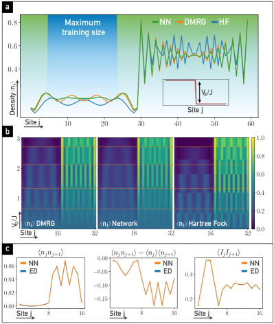
Figure 2: Performance of the network addressing the interplay of interactions and interference. (a) Density for a step potential (never seen during training), displaying Friedel oscillations in a 1D system of interacting fermions. The NN prediction is very close to the almost exact result (DMRG), in contrast to Hartree-Fock. (b) Density evolution vs. potential step height, comparing the three different approaches; again the NN performs very well. (c) Predictions for multiple observables, obtained from the single (multi-head) network, evaluated for a step potential in a smaller system size. We compare the network output with the exact diagonalization (ED) result.

We observe a very good match with DMRG predictions, while Hartree-Fock struggles and gives unreliable results. This is particularly apparent when sweeping the potential step height. That leads to characteristic step-wise changes in the total particle number contained in the potential well and resulting changes in the density-dependent wave length of the oscillations. These are captured well by the network – even though to do so the network has to extract non-local information, since the particle number quantization depends on the extent of the well. In this example of interacting 1D fermionic systems, we also take the opportunity to train and predict multiple observables, as recounted above. In addition to observables connected to the density $\hat{n}$, we predict the current between sites, $\hat{I}(x)=iJ(\hat{a}^{\dagger}(x-\delta x)\hat{a}(x)-\hat{a}^{\dagger}(x)\hat{a}(x-\delta x))$, and its correlator. In this case, we compare the NN predictions vs. exact diagonalization (choosing a smaller lattice size for that purpose) and observe an extremely close match (Fig. 2c). We have verified that training samples are not close to the test potential.

The second main characteristic of inhomogeneous quantum many-body systems, beyond the interplay of interference and interactions, is the appearance of phase transitions and the resulting spatial patterns of different phases produced in an external potential. A correct predictive approach must not only reproduce the homogeneous bulk phase diagram but also be able to capture features in inhomogeneous scenarios, like finite penetration depths observed at domains walls separating different phases in space and the strongly modified response to local perturbations when the system is close to a phase boundary.

We have investigated the performance of our deep-learning approach for a paradigmatic 2D model system, the bosonic Hubbard model. Specifically, we selected the extended model with both onsite and nearest-neighbor interactions. This model Ohgoe et al. (2012); Suthar et al. (2020) is known to have multiple phases, including the homogeneous Mott insulator and superfluid, but also phases with a spontaneously arising periodic density modulation (checkerboard and supersolid phases). The Hamiltonian for this model is given by

$$\begin{split}{\hat{H}}=&-J\sum_{x,x^{\prime}}{\hat{a}}^{\dagger}(x){\hat{a}}(x^{\prime})\\ &+{U\over 2}\sum_{x}{\hat{n}}(x)({\hat{n}}(x)-1)\\ &+U^{\prime}\sum_{x,x^{\prime}}{\hat{n}}(x){\hat{n}}(x^{\prime})+\sum_{x}(V(x)-\mu){\hat{n}}(x).\end{split}$$ (2)

Here $U$ and $U^{\prime}$ are the onsite and nearest-neighbor interactions, respectively, and the sum over $x^{\prime}$ is assumed to range over all nearest neighbors of $x$. In this example, we want to learn not only for a given model, with fixed interactions, but rather be able to make predictions for a whole class of models. To this end, during training we choose $U$ and $U^{\prime}$ for each sample randomly, within certain ranges. As explained above, the values of these parameters are fed into the network in the form of spatially constant additional input channels. By training in this way on a range of parameters, the network profits from its ability to interpolate, i.e. all the observed samples will provide useful information even for predictions eventually extracted at other parameter combinations.

A particular challenge for NN training is produced when a phase has a spontaneously broken symmetry, since the predictions for a given potential can assume one of several outcomes, which would confuse the network. This general aspect is illustrated nicely for the case of the checkerboard solid, which shows a staggered density. In contrast, the spontaneously broken U(1) symmetry for the superfluid does not affect the observables we consider. To cope with this challenge, during training we additionally supply the network with an extra channel, that effectively selects the broken symmetry sector. Specifically for the checkerboard, we provide another channel as input to the network, which contains the checkerboard variant (one of two), which is most strongly correlated with the observed density. This is even necessary for inhomogeneous potentials, since QMC does not reliably pick the energetically slightly favourable variant.

We train on predictions obtained using finite-temperature QMC on relatively small systems with an even number of sites $L\in\{6,8,10,12,14,16\}$ using the worm algorithm Troyer et al. (2003). For the training, we create data sets of up to 170,000 samples, though we checked that already 2,000 samples lead to very good results (see Fig. 3f). Further details about the data generation can be found in the appendix.

As training is performed on random potentials, a non-trivial check on the accuracy of the resulting trained network can already be obtained by using the network to predict the phases of homogeneous situations. The resulting phase diagram is shown in Fig. 3a, with a very good match against QMC predictions. Moving beyond bulk phases, we test predictions for inhomogeneous situations. In the first example, we choose a parabolic potential underlying the lattice, which is a typical situation in experiments with ultracold atoms in optical lattices. The resulting characteristic stepwise density distribution (in the case of the standard bosonic Hubbard model with Mott and superfluid phases) is known as a ’wedding cake’ structure. In the present case as shown in Fig. 3d, there are more phases visible, and we compare against QMC predictions. In a second example depicted in Fig. 3c, we take a square potential well, and we study the resulting density distribution vs. a varying potential depth, again performing a comparison against the numerically exact QMC result.

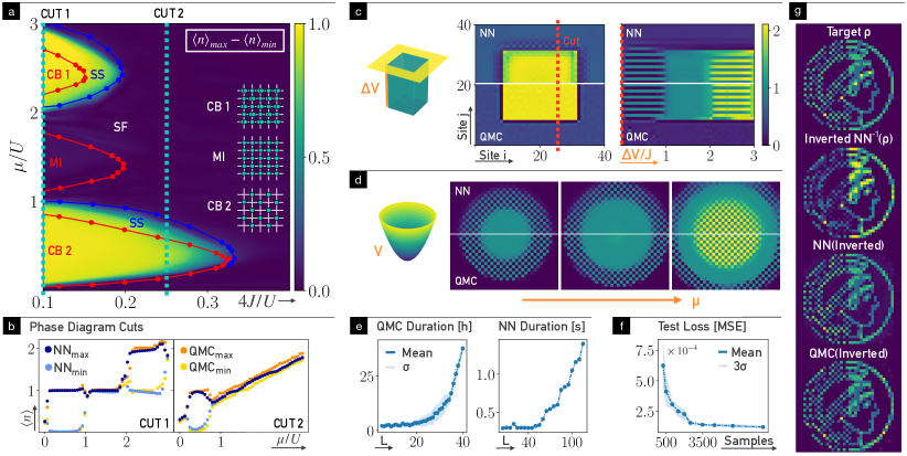
Figure 3: Results for a 2D model with phase transitions. (a) Phase diagram for the 2D Hubbard model with nearest-neighbor coupling, vs. chemical potential and hopping strength for $4U^{\prime}/U=1.0$. The NN (trained on finite-T QMC results) is asked to predict the density for a flat potential, after having been trained on random potentials. We plot the difference between the maximum and the minimum of the density. The indicated phase boundaries mark the ground-state phase transitions extracted from Ohgoe et al. (2012). Checkerboard solids $\textrm{CB}_{1}$ and $\textrm{CB}_{2}$ with filling factors $\rho=3/2,1/2$, supersolid (SS), superfluid (SF), Mott insulator (MI, $\rho=1$). (b) Cuts through (a), comparing predictions of the network with those obtained from QMC (with max. and min. densities). QMC densities in the SF phase are not perfectly constant in space, due to sampling noise. (c) Predictions (NN vs. QMC) for a 2D potential well. Right plot shows evolution of density along a 1D cut for varying well depth. (d) Predictions for a harmonic potential, changing the chemical potential. (e) Wall-clock time for QMC calculations vs. system size (for a fixed convergence criterion), and the same for NN evaluation (inference time). (f) Test error (mean squared error) vs. training set size, indicating fluctuations (standard deviation $\sigma$) over several training runs. (g) For given parameters (4J/U=0.3,zU’/U=1.0) the network (NN) is used to ”invert” a prescribed density $\rho$ to produce a corresponding potential (Inverted), see main text, which is tested by using both the NN and QMC for recovering the density.

Having trained a neural network for the task of predicting inhomogeneous quantum many-body systems, the most straightforward benefit is speed, enabling application to large-scale systems. We illustrate this by comparing the time it takes to run QMC simulations vs. the time it takes the neural network to produce predictions, as a function of the system size (Fig. 3e). Even though such a comparison comes with caveats – e.g. the time needed to run QMC for a given potential depends on the details of the convergence criteria adopted – it is clear that there is a difference of many orders of magnitude, and this observation is independent of such details. Specifically for system size 40, we achieve a speed up of a factor of $5\cdot 10^{5}$, which is likely even more pronounced for larger systems, as the NN inference time scales much more favorably with the system size. Another important aspect, besides inference time, is the time it takes to generate training samples using expensive techniques like QMC. In Fig. 3f, we show the test loss as a function of the number of training samples, observing that even for a few thousand samples the loss is already on the same order of magnitude as for $10^{5}$ samples. This is a very important message for the feasibility of the whole method.

Another important benefit of using a network is that it represents a differentiable mapping from input to output. This can be exploited for inverse design. For that purpose, we would start from a given desired observable map (e.g. a density distribution), or, more generally, some cost function that prefers certain features in the predicted observable map. We can then take the derivative of that cost function with respect to the input, i.e. with respect to the underlying potential (or the model parameters), in order to do gradient descent and find the potential landscape that is able to produce the desired effect. Here we constrain the inversion to ranges the network was previously trained on, by applying gradient descent to an unconstrained input variable, which is mapped to a constrained network input by an accordingly scaled and shifted sigmoid function. In some cases, there may be a continuum of possible solutions, in other cases - possibly due to the constrained nature of the inversion - one might only find a compromise solution, i.e. come as close as possible to the desired output. We illustrate this use case in Fig. 3g.

In conclusion, we have shown how a deep neural network can efficiently predict inhomogeneous densities in large-scale quantum many-body systems, including aspects like simultaneous treatment of multiple observables. With this technique, one can speed up the exploration of designed potentials by several orders of magnitude and apply inverse design to obtain desired outcomes. Another promising future application would be Hamiltonian learning, deducing the potential and model parameters from experimental observations in the ground state of a system. While we have trained on simulations, modern developments will enable training on experimental data, most notably using quantum gas microscopes for optical lattices which also enable local potential programming Gross and Bakr (2021).

I Appendix

I.1 Training Data Generation

In the 1D examples, we trained on potentials $V(x)$ that are realizations of uniform white noise ($\overline{V(x)V(x^{\prime})}=\delta_{x,x^{\prime}}$) with $V(x)/J\in[-12,12]$. The input for the network was solely the combination $V(x)-\mu$, where $\mu$ is extracted from the energy dependence on the number of particles, as described in the main text.

For the 2D example, we instead used Gaussian colored noise. This means the potential $V(x)$ was obtained using inverse Fourier transformation starting from randomly chosen complex Fourier amplitudes with a fall-off towards higher wavenumbers. Given the chemical potential $\mu$, we then for a random amplitude $A\in[0,|\mu|/2]$ shift and rescale V, such that $\max_{x}{V(x)}-\min_{x}{V(x)}=2A$ and $\overline{V(x)}=0$.

In addition, in the 2D example, we supply the model parameters in the Hamiltonian as input channels to the network. For the training set, these parameters were drawn from uniform distributions. In particular, we selected $4J/U\in[0.05,1]$, where the hopping strength $J$ is set to one, $4U^{\prime}/U\in[0.75,1.75]$ and ultimately $\mu\in[-0.5U,3U]$.

For the QMC application, we limit the number of particles per site to three and run the worm algorithm for $10^{7}$ sweeps at temperature $T/J=1.0$.

I.2 Network Architecture

As a starting point for the network architecture, we use standard convolutions with kernel size five as the first layer and kernel size three for all following layers, without pooling and with strides set to one (i.e. keeping the same resolution). All convolutions wrap around the input periodically, such that we effectively mimic periodic boundary conditions for the network’s analysis.

In order to be able to correlate as many sites as possible, we design the networks to be rather deep (see below), since stacked convolutions extend the capability to learn long-range correlations. To facilitate the training we employ residual connections He et al. (2015) and batch norms Ioffe and Szegedy (2015). As non-linear activation ReLU is used. The training proceeded with the standard Adam optimizer. In principle any point-wise cost function is suitable, but we used the mean absolute error (MAE) for the one-dimensional model and the mean squared error (MSE) in the two-dimensional case.

Ultimately, after exploring several design choices and hyperparameters, we selected the model with the smallest validation loss for our studies.

For the one-dimensional model, we found that a ResNet-type architecture with 64 blocks produces the best results. Opposed to the common ResNet design, we did not include dropout and pooling operations. Every layer produces 120 output channels. The best performing architecture for the two-dimensional system was a purely convolutional neural network with 20 layers and 200 channels per layer. This seems to be mainly due to better resilience to the rather noisy dataset built with QMC.

For model architectures and additional tasks like the inversion, our implementations rely on Pytorch PyT .

References

- Carrasquilla (2020) J. Carrasquilla, Advances in Physics: X 5, 1797528 (2020).
- Carleo et al. (2019) G. Carleo, I. Cirac, K. Cranmer, L. Daudet, M. Schuld, N. Tishby, L. Vogt-Maranto, and L. Zdeborová, Reviews of Modern Physics 91, 045002 (2019).
- Dawid et al. (2022) A. Dawid, J. Arnold, B. Requena, A. Gresch, M. Płodzień, K. Donatella, K. A. Nicoli, P. Stornati, R. Koch, M. Büttner, R. Okuła, G. Muñoz-Gil, R. A. Vargas-Hernández, A. Cervera-Lierta, J. Carrasquilla, V. Dunjko, M. Gabrié, P. Huembeli, E. van Nieuwenburg, F. Vicentini, L. Wang, S. J. Wetzel, G. Carleo, E. Greplová, R. Krems, F. Marquardt, M. Tomza, M. Lewenstein, and A. Dauphin, arXiv:2204.04198 [cond-mat, physics:quant-ph] .
- Carleo and Troyer (2017) G. Carleo and M. Troyer, Science 355, 602 (2017).
- Schmitt and Heyl (2020) M. Schmitt and M. Heyl, Physical Review Letters 125, 100503 (2020).
- Hartmann and Carleo (2019) M. J. Hartmann and G. Carleo, Physical Review Letters 122, 250502 (2019), arXiv:1902.05131 [cond-mat, physics:quant-ph] .
- Brockherde et al. (2017) F. Brockherde, L. Vogt, L. Li, M. E. Tuckerman, K. Burke, and K.-R. Müller, Nature Communications 8, 872 (2017).
- Costa et al. (2022) E. Costa, G. Scriva, R. Fazio, and S. Pilati, arXiv:2205.08367 [cond-mat, physics:physics] .
- Chandrasekaran et al. (2019) A. Chandrasekaran, D. Kamal, R. Batra, C. Kim, L. Chen, and R. Ramprasad, npj Computational Materials 5, 22 (2019).
- Ryczko et al. (2019) K. Ryczko, D. Strubbe, and I. Tamblyn, Physical Review A 100, 022512 (2019), arXiv:1811.08928 .
- Nelson et al. (2019) J. Nelson, R. Tiwari, and S. Sanvito, Physical Review B 99, 075132 (2019), arXiv:1810.12700 .
- Moreno et al. (2019) J. R. Moreno, G. Carleo, and A. Georges, arXiv:1911.03580 [cond-mat, physics:quant-ph] (2019), arXiv:1911.03580 [cond-mat, physics:quant-ph] .
- Behler and Parrinello (2007) J. Behler and M. Parrinello, Physical Review Letters 98, 146401 (2007).
- Bartók et al. (2017) A. P. Bartók, S. De, C. Poelking, N. Bernstein, J. R. Kermode, G. Csányi, and M. Ceriotti, Science Advances 3, e1701816 (2017).
- Valenti et al. (2019) A. Valenti, E. van Nieuwenburg, S. Huber, and E. Greplova, Physical Review Research 1, 033092 (2019).
- Saraceni et al. (2020) N. Saraceni, S. Cantori, and S. Pilati, Physical Review E 102, 033301 (2020).
- Mujal et al. (2021) P. Mujal, À. Martínez Miguel, A. Polls, B. Juliá-Díaz, and S. Pilati, SciPost Physics 10, 073 (2021).
- Gresch et al. (2022) A. Gresch, L. Bittel, and M. Kliesch, arXiv:2202.08853 [cond-mat, physics:quant-ph] .
- Mohseni et al. (2022) N. Mohseni, T. Fösel, L. Guo, C. Navarrete-Benlloch, and F. Marquardt, Quantum 6, 714 (2022), arXiv:2105.00352 [quant-ph] .
- He et al. (2015) K. He, X. Zhang, S. Ren, and J. Sun, arXiv:1512.03385 [cs] .
- Fishman et al. (2022) M. Fishman, S. White, and E. Stoudenmire, SciPost Physics Codebases , 4 (2022).
- Ohgoe et al. (2012) T. Ohgoe, T. Suzuki, and N. Kawashima, Physical Review B 86, 054520 (2012), arXiv:1206.3670 [cond-mat] .
- Suthar et al. (2020) K. Suthar, H. Sable, R. Bai, S. Bandyopadhyay, S. Pal, and D. Angom, Physical Review A 102, 013320 (2020), arXiv:1904.12649 [cond-mat] .
- Troyer et al. (2003) M. Troyer, F. Alet, S. Trebst, and S. Wessel, AIP Conference Proceedings 690, 156 (2003).
- Gross and Bakr (2021) C. Gross and W. S. Bakr, Nature Physics 17, 1316 (2021).
- Ioffe and Szegedy (2015) S. Ioffe and C. Szegedy, arXiv:1502.03167 [cs] .
- (27) PyTorch, https://www.pytorch.org.