Discrete defect plasticity and implications for dissipation

Abstract

Inelastic deformation of solids is almost always, if not always, associated with the evolution of discrete defects such as dislocations, vacancies, twins and shear transformation zones. The focus here is on discrete defects that can be modeled appropriately by continuum mechanics, but where the discreteness of the carriers of plastic deformation plays a significant role. The formulations are restricted to small deformation kinematics and the defects considered, dislocations and discrete shear transformation zones (STZs), are described by their linear elastic fields. In discrete defect plasticity both the stress-strain response and the partitioning between defect energy storage and defect dissipation are outcomes of an initial/boundary value problem solution. For such defects an explicit expression for the dissipation rate is presented and, because there is a length scale associated with the discrete defects, the stress-strain response and the evolution of the dissipation rate can be size dependent. Discrete dislocation plasticity modeling results are reviewed that illustrate the implications of defect dissipation evolution for friction, fracture, fatigue crack growth and thermal softening. Examples are also given of the consequences in constrained shear of three modes of the evolution of discrete defects for the size dependence of the stress-strain response and the associated dissipation. For a purely mechanical formulation the Clausius-Duhem inequality specializes to the requirement that the dissipation rate is non-negative. Requiring a non-negative dissipation rate for all points of a body and for all time imposes restrictions on kinetic relations for the evolution of discrete defects. In statistical mechanics, the Clausius-Duhem inequality can be violated for sufficiently small regions for a sufficiently short time. Explicit kinetic relations for discrete dislocation plasticity dissipation and for discrete STZ plasticity dissipation identify conditions that can lead to a negative dissipation rate. In continuum mechanics, at least in some circumstances, satisfaction of the Clausius-Duhem inequality can be regarded as a stability requirement. Nevertheless, simple one-dimensional continuum calculations illustrate that there can be a negative dissipation rate over a small region and for a short time period with overall stability maintained. Implications for discrete defect plasticity modeling are briefly discussed.

1 Introduction

Inelastic deformation of solids generally takes place by the evolution in space and time of a collection of discrete defects such as dislocations, vacancies, phase transformations, twins, and shear transformation zones (STZs). A variety of deformation and failure processes are governed by the evolution of collections of such defects, in many circumstances each of which can be modeled appropriately by continuum mechanics, but where the discreteness of the carriers of plastic deformation plays a significant role. Discrete defect effects can be key for modeling structure/component performance and reliability for both micro-scale and macro-scale components and devices. In particular, discrete defects dissipate energy and store energy, and the balance between dissipation and energy storage plays a key role in a variety of phenomena of technological significance including, for example, thermal softening, friction, fracture and fatigue.

As for any continuum formulation, in addition to satisfying basic principles, i.e. the kinematics of deformation and the conservation of mass, momentum and energy, constitutive relations (in this context termed kinetic relations) are needed for modeling the discrete defects. In discrete defect plasticity, the stress-strain response is an outcome of an initial/boundary value problem solution (not an input as in conventional continuum plasticity) as is the partitioning between defect energy storage and defect dissipation. Furthermore, there is a length scale associated with discrete defects, for example, the Burgers vector for a dislocation or size associated with a shear transformation zone (STZ), so that both the stress-strain response and the evolution of the energy partitioning can be size dependent.

A proper continuum mechanics formulation is also expected to satisfy a statement (or perhaps more accurately one of the statements) of the second law of thermodynamics. The statement of the second law in terms of satisfying the Clausius-Duhem inequality for all points of a body for all time was introduced as a postulate into continuum mechanics by Coleman and Noll (1964) and provides a formalism for developing constitutive relations consistent with that inequality for all time. In discrete defect plasticity, satisfaction of the Coleman-Noll postulate, i.e. requiring the dissipation rate to be non-negative for all material regions and for all time, places a restriction on the kinetic relations for defect evolution.

Satisfaction of the Coleman-Noll postulate (Coleman and Noll, 1964) is well-established for macro-scale continuum modeling. In statistical mechanics this requirement emerges for large systems and long periods of time, Evans and Searles (2002); Jarzynski (2010). However, theoretical, computational and experimental studies have shown that, when the process under consideration involves a sufficiently small region for a sufficiently short time, satisfying the Clausius-Duhem inequality has a probability less than one, e.g. Evans et al. (1993); Ayton et al. (2001); Evans and Searles (2002); Jarzynski (2010); Wang et al. (2010); Ostoja-Starzewski and Laudani (2020). This may be relevant for discrete defect plasticity since the change in defect state may only involve a small number of discrete entities in a sufficiently small material region and may occur over a sufficiently short time. Key issues, of course, are what is “sufficiently small” and what is “sufficiently short.”

We begin with a brief presentation of the Clausius-Duhem inequality and illustrate the implications of requiring satisfaction of the Coleman-Noll postulate (Coleman and Noll, 1964) for constitutive relations in conventional continuum mechanics. A continuum mechanics framework is then outlined for solving problems with plastic deformation arising from the evolution of discrete defects. The continuum mechanics framework is restricted to small deformations (i.e. geometry changes neglected) and attention is focused on defects, such as dislocations and shear transformation zones (STZs), that can be described in terms of their linear elastic fields; $1/r$ singular strain/stress fields for dislocations and Eshelby (1957, 1959) inclusion fields for STZs. For such defects, dissipation only occurs on surfaces with displacement/displacement rate jumps.

Explicit expressions for the dissipation rate for discrete dislocation plasticity and for discrete STZ plasticity are given. Particular attention is directed to restrictions imposed on discrete defect kinetic relations by requiring the dissipation rate to be non-negative. In addition, results are presented of discrete dislocation plasticity analyses that illustrate the implications of the evolution of defect dissipation for friction, fatigue crack growth and the development of the Bauschinger effect and thermal softening in plane strain tension. These results illustrate what can be predicted by discrete dislocation modeling, with the dissipation rate being non-negative for all time, for the evolution of dissipation, for its size dependence and for the resulting effect on material response.

For STZ plasticity, the requirement of a non-negative dissipation rate for all time restricts the transformation strain magnitude to be smaller than indicated by atomistic analyses and experiment, e.g. Argon and Shi (1983); Dasgupta et al. (2013); Albert et al. (2016); Hufnagel et al. (2016). Possible reasons for this discrepancy include: (i) nonlinear elastic/non-elastic material behavior; (ii) identifying the Eshelby (1957, 1959) inclusion transformation stress with the yield strength and not accounting for possible local stress concentrations; (iii) neglecting the role of entropy, particularly configurational entropy; and (iv) this could be a circumstance where the Clausius-Duhem inequality can be violated for a small number of discrete entities and a short time.

Discrete STZ plasticity predictions are presented for the stress-strain response and for the spatial stress, strain and dissipation distributions in plane strain tension with the formulation satisfying the requirement of a non-negative dissipation rate for all STZs for all time.

Examples are given of consequences for the size dependence of the stress-strain response and for the size dependence of plastic dissipation of three modes of evolution of discrete defects: (i) relatively few defects that move relatively long distances through the material; (ii) nucleation of defects from fixed nucleation sites with the nucleated defects moving only short distances or not all; and (iii) nucleation of defects that do not move but that induce a percolation-like increase in the number of nucleation sites. Each of these leads to a different prediction for the size dependence of the stress-strain response and of the associated dissipation.

The more general question of the consequences of violating Clausius-Duhem inequality in a continuum formulation (for a purely mechanical framework violating the requirement of a non-negative dissipation rate) for a short time is explored in a simple one-dimensional context and possible implications for discrete defect plasticity modeling are briefly discussed.

2 The Clausius-Duhem inequality and dissipation

Attention is restricted to small deformation kinematics and quasi-static processes (kinetic energy negligible). Using Cartesian tensor notation, the strain tensor components, $\epsilon_{ij}$, are given by

$$\epsilon_{ij}=\frac{1}{2}\left(u_{i,j}+u_{j,i}\right)$$ (1)

with $u_{i}$ the components of the displacement vector, and $(\_)_{,i}$ denotes $\partial(\ )/\partial x_{i}$. Also, the stress tensor components, $\sigma_{ij}$ satisfy

$$\sigma_{ij,j}=0$$ (2)

so that

$$\int_{V}\sigma_{ij}{\dot{\epsilon}}_{ij}dV=\oint_{S}\sigma_{ij}n_{j}\dot{u}_{i}dS$$ (3)

where $V$ is the volume of the body, $S$ is the surface of $V$, $n_{j}$ are the components of the unit normal to $S$ and $(\dot{\ })=\partial{(\ )}/{\partial t}$.

The only non-mechanical fields considered are the temperature $\Theta$, the entropy $s$, and the heat flux vector ${\bf q}$. In this context, the Clausius-Duhem inequality for a body with volume $V$ then can be written as (Coleman and Noll, 1964)

$$\dot{W}-\dot{\Phi}+\int_{V}\Theta\dot{s}dV-\int_{V}\left(\frac{q_{i}}{\Theta}\right)\Theta_{,i}dV\geq 0$$ (4)

where $\dot{W}$ is the rate of working and $\dot{\Phi}$ is the time derivative of the internal energy, with

$$\dot{W}=\oint_{S}\sigma_{ij}n_{j}\dot{u}_{i}dS=\int_{V}\sigma_{ij}{\dot{\epsilon}}_{ij}dV=\int_{V}\dot{w}dV\quad,\quad\dot{\Phi}=\int_{V}\dot{\phi}dV$$ (5)

In the context of a small deformation framework $\dot{w}$ and $\dot{\phi}$ are taken to be per unit volume (rather than per unit mass).

If the Clausius-Duhem inequality, Eq. (4), is presumed to hold for any admissible deformation and thermal history, and for any sub-volume, then at each point of $V$

$$\sigma_{ij}{\dot{\epsilon}}_{ij}-\dot{\phi}+\Theta\dot{s}-\left(\frac{q_{i}}{\Theta}\right)\Theta_{,i}\geq 0$$ (6)

Note that if Eq.(6) holds at then at each point of $V$, then Eq.(4) holds. However, Eq.(4) can hold even if Eq.(6) does not hold at each point of $V$.

One example of the implications of requiring satisfaction of the Clausius-Duhem inequality, Eq. (6), for all points of the body and for all time, i.e. satisfying the Coleman-Noll postulate (Coleman and Noll, 1964), is illustrated by taking $\phi(\epsilon_{ij},s)$ so that

$$\dot{\phi}=\frac{\partial\phi}{\partial\epsilon_{ij}}\dot{\epsilon}_{ij}+\frac{\partial\phi}{\partial s}\dot{s}$$ (7)

Substituting Eq. (7) into Eq. (6) gives

$$\left[\sigma_{ij}-\frac{\partial\phi}{\partial\epsilon_{ij}}\right]{\dot{\epsilon}}_{ij}+\left[\Theta-\frac{\partial\phi}{\partial s}\right]\dot{s}-\left(\frac{q_{i}}{\Theta}\right)\Theta_{,i}\geq 0$$ (8)

Because Eq. (8) must hold for any admissible history, it must hold if any two of ${\dot{\epsilon}}_{ij}$, $\dot{s}$, $\Theta_{,i}$ vanish. Hence, Eq. (8) requires

$$\sigma_{ij}=\frac{\partial\phi}{\partial\epsilon_{ij}}\quad,\quad\Theta=\frac{\partial\phi}{\partial s}\quad,\quad-\left(\frac{q_{i}}{\Theta}\right)\Theta_{,i}\geq 0$$ (9)

With the focus on a purely mechanical framework so that entropy and heat flux/temperature gradient effects are not included in the formulation, Eq. (4) simplifies to

$$\dot{\cal D}=\dot{W}-\dot{\Phi}\geq 0$$ (10)

and Eq. (6) becomes

$$\dot{\xi}=\sigma_{ij}{\dot{\epsilon}}_{ij}-\dot{\phi}\geq 0$$ (11)

where $\dot{\cal D}$ is the dissipation rate in the body and $\dot{\xi}$ is the dissipation per unit volume.

We consider a class of elastic-plastic or an elastic-viscoplastic solids for which

$$\dot{\epsilon}_{ij}=\dot{\epsilon}^{e}_{ij}+\dot{\epsilon}^{p}_{ij}$$ (12)

and

$$\dot{\epsilon}^{p}_{ij}=\dot{\Lambda}q_{ij}$$ (13)

Assuming that plastic deformation makes no contribution to the internal energy so that $\dot{\phi}=\sigma_{ij}\dot{\epsilon}^{e}_{ij}$, the local Clausius-Duhem inequality, Eq. (11), then requires

$$\dot{\xi}=\sigma_{ij}\dot{\epsilon}^{e}_{ij}+\sigma_{ij}\dot{\epsilon}^{p}_{ij}-\dot{\phi}=\sigma_{ij}\dot{\epsilon}^{p}_{ij}=\dot{\Lambda}\sigma_{ij}q_{ij}\geq 0$$ (14)

and the Clausius-Duhem inequality is satisfied for all deformation histories and all time if $\dot{\Lambda}\geq 0$ and $\sigma_{ij}q_{ij}\geq 0$.

For example, if

$$q_{ij}=\sigma_{ij}^{\prime}+\alpha\sigma_{kk}\delta_{ij}$$ (15)

so that

$$\sigma_{ij}q_{ij}=\left[\sigma_{ij}^{\prime}\sigma_{ij}^{\prime}+\alpha\sigma^{2}_{kk}\right]$$ (16)

where $\delta_{ij}$ is the Kronecker delta and $\sigma_{ij}^{\prime}=\sigma_{ij}-1/3\sigma_{kk}\delta_{ij}$, then with $\dot{\Lambda}\geq 0$, the Clausius-Duhem inequality is satisfied for all stress states if $\alpha\geq 0$.

The statement that the Clausius-Duhem inequality, Eq. (6), must be satisfied for all points of a body and for all deformation and thermal histories is basically taken as a postulate by Coleman and Noll (1964) so the question arises as to what are the implications of it not being satisfied. It has been shown that satisfaction of the Clausius-Duhem inequality implies stability at least in some cases, for example, Lyapunov stability for systems with time evolution governed by ordinary differential equations, Coleman and Mizel (1967), or continuous dependence of thermodynamic processes on the initial state and supply terms terms for thermoelastic materials, Dafermos (1979). A possibility is that more generally violation of the Clausius-Duhem inequality (in a purely mechanical formulation having a negative dissipation rate) will lead to some kind of instability.

3 Discrete defect plasticity

At a size scale where the discreteness of defects plays a role, plastic deformation is inevitably nonuniform. In a wide variety of circumstances, the evolution of collections of such defects can be modeled appropriately within a continuum mechanics framework. Within such a framework, the stress strain response and the evolution of the material microstructure are direct outcomes of an initial/boundary value problem solution. A possible size effect of the stress-strain response and of the energy partitioning, as well as their dependence on stress state, loading rate, deformation history, etc. is also an outcome.

The aims of discrete defect plasticity analyses are: (i) to provide predictions of the mechanical response of materials that are difficult, if not impossible, to obtain from smaller scale or larger scale frameworks; and/or (ii) to provide guidance for developing continuum plasticity constitutive relations.

Although the general formulation applies to a range of discrete defects, attention here is focused dislocations and shear transformation zones (STZs). Both are modeled in terms of their linear elastic fields but have quite different behaviors. Dislocations are mobile and give rise to long range stresses. On the other hand, the positions of STZs are fixed and their associated stress fields have a shorter range than those of dislocations.

3.1 Modeling framework

In addition to consideration being restricted to small deformation kinematics and quasi-static deformation histories, in the specific situations considered, the stress and strain are taken to be related by linear isotropic elasticity, so that

$$\sigma_{ij}=L_{ijkl}\epsilon_{kl}=\frac{E}{(1+\nu)}\left[\epsilon_{ij}+\frac{\nu}{1-2\nu}\epsilon_{kk}\delta_{ij}\right]$$ (17)

with $L_{ijkl}=L_{klij}$ the components of the tensor of elastic moduli, $E$ Young’s modulus, $\nu$ Poisson’s ratio. Also, for a purely mechanical formulation, the elastic energy per unit volume is

$$\phi(\epsilon_{ij})=\frac{1}{2}L_{ijkl}\epsilon_{ij}\epsilon_{kl}=\frac{1}{2}\sigma_{ij}\epsilon_{ij}$$ (18)

Figure 1: Illustration of the superposition-based boundary value problem solution for a body containing discrete defects. The $(\tilde{\ })$ fields correspond to the discrete defect fields in an infinite body and the $(\hat{\ })$ fields are the image fields that are obtained to satisfy the imposed boundary conditions.

The superposition procedure for solving boundary value problems with a collection of discrete defects introduced by Van der Giessen and Needleman (1995) is sketched in Fig. 1. A collection of discrete defects is assumed present in the solid. Each defect is associated with am equilibrium stress field and a displacement field. At any time $t$, the stress $\tilde{\sigma}_{ij}(t)$ and displacement $\tilde{u}_{i}(t)$ fields associated with the collection of defects can be written as

$$\tilde{\sigma}_{ij}(t)=\sum_{K=1}^{N}\sigma^{K}_{ij}(t)$$ (19a)

$$\tilde{u}_{i}(t)=\sum_{K=1}^{N}u^{K}_{i}(t)$$ (19b)

where $N$ is the number of discrete defects and for each defect equilibrium stress field $\sigma^{K}_{ij,j}=0$. Although the stress and deformation fields are associated with a solution to a linear elastic boundary value problem, they are not necessarily smooth. Indeed, in general, each displacement field $u^{K}_{i}(t)$ is only piecewise differentiable and the corresponding stress field $\sigma^{K}_{ij}(t)$ may be singular, as for a dislocation.

The $(\tilde{\ })$ stress and displacement fields are presumed to be described by linear elasticity theory and known either from analytical expressions or from some separate semi-numerical computation. The boundary conditions used to obtain the individual defect fields are chosen for convenience, for example, for a defect in an infinite or semi-infinite solid. Hence, the $\tilde{\sigma}_{ij}$ and $\tilde{u}_{i}$ fields do not meet the imposed boundary conditions

$$T_{i}(t)=\sigma_{ij}n_{j}=T_{i}^{0}(t)\ {\rm on}\ S_{T}\quad,\quad u_{i}(t)=u_{i}^{0}(t)\ {\rm on}\ S_{u}$$ (20)

where $T_{i}^{0}(t)$ are the imposed traction vector components on $S_{T}$ and $u_{i}^{0}(t)$ are the imposed displacement components on $S_{u}$.

In order to meet the boundary conditions, the stress field $\hat{\sigma}_{ij}(t)$ and the displacement field $\hat{u}_{i}(t)$ are introduced. The $(\hat{\ })$ fields are image fields and have no singularities in the body under consideration even if $\tilde{\ }$ fields do. The $(\hat{\ })$ fields are determined from the solution to the boundary value problem

$$\hat{\sigma}_{ij,j}=0$$ (21)

with the boundary conditions

$$\hat{T}_{i}(t)=\hat{\sigma}_{ij}n_{j}=(T_{i}^{0}(t)-\tilde{T}_{i})\ {\rm on}\ S_{T}\quad,\quad\hat{u}_{i}(t)=(u_{i}^{0}(t)-\tilde{u}_{i})\ {\rm on}\ S_{u}$$ (22)

and $\hat{\sigma}_{ij}(t)=L_{ijkl}\hat{\epsilon}_{ij}(t)$. Eqs. (21) and (22) constitute a standard linear elasticity problem that can be solved numerically by a variety of methods, including the finite element method, a boundary element method, a spectral method, etc.

As illustrated in Fig. 1, the total stress and displacement fields are determined by superposition,

$$\sigma_{ij}(t)=\hat{\sigma}_{ij}(t)+\tilde{\sigma}_{ij}(t)$$ (23)

$$u_{i}(t)=\hat{u_{i}}(t)+\tilde{u_{i}}(t)$$ (24)

and satisfy the governing equations and the imposed boundary conditions.

The $(\hat{\ })$ fields generally vary more slowly spatially than the $(\tilde{\ })$ fields so that an advantage of this superposition method is that in a numerical solution, a much coarser discretization can be used than if the $(\tilde{\ })$ fields needed to be directly solved for in the calculation.

Note that in general it is not necessary for all defects to be of the same kind but this superposition procedure can, in principle, be used for some combination of dislocations, shear transformation zones, vacancies, etc.

3.2 Dissipation rate for discrete defect plasticity

The Clausius-Duhem inequality for a purely mechanical formulation is expressed by Eq. (10) and the elastic energy per unit volume is given by Eq. (18). Attention is confined to circumstances where the defect fields are described by linear elasticity. The boundary correction (or image) fields, $(\hat{\ })$, are continuous and appropriately differentiable in $V$. However, the $(\tilde{\ })$ fields can have surfaces of displacement/displacement rate discontinuity as, for example, for dislocation fields and for Eshelby (1957, 1959) transformation fields. The displacement/displacement rate discontinuities are then what give rise to plastic deformation/plastic deformation rate.

Using a decomposition similar to Eq. (23) for the strain rate $\dot{\epsilon}_{ij}$ $\dot{\tilde{\epsilon}}_{ij}$ is expressed in terms of the $K=1,2,...N$ individual defect strain rate fields as

$$\dot{\tilde{\epsilon}}_{ij}=\sum_{K}\dot{\tilde{\epsilon}}^{K}_{ij}$$

and $\dot{W}$ is given by

$$\dot{W}=\dot{W}_{\rm ext}+\sum_{S^{K}}\dot{W}^{K}=\int_{S_{\rm ext}}T_{i}\dot{u}_{i}dS+\sum_{S^{K}}\dot{W}^{K}=\int_{V_{e}}\sigma_{ij}\left(\dot{\hat{\epsilon}}_{ij}+\sum_{K}\dot{\epsilon}^{K}_{ij}\right)dV+\sum_{S^{K}}\dot{W}^{K}$$ (25)

where $T_{i}=\sigma_{ij}n_{j}$ are the traction vector components, $S_{\rm ext}$ is the external surface with normal $n_{j}$, $\sigma_{ij}$ and $\dot{u}_{i}$ are given by Eqs. (23) and (24), respectively, $S^{K}$ is the surface of discontinuity in $V$ associated with defect $K$, ${\dot{W}}^{K}$ is the work rate on $S^{K}$, $\dot{W}_{\rm ext}$ is the work rate on the external surface of $V$ and $V_{e}$ denotes the volume of the material not including the $K=1,2,...N$ surfaces $S^{K}$.

The elastic energy rate per unit volume is given by $\dot{\phi}=\sigma_{ij}\dot{\epsilon}_{ij}$ in the material volume (which is where $\dot{\epsilon}_{ij}$ is defined) and the dissipation rate for defect $K$ is the work rate $\dot{W}^{K}$ on its associated discontinuity surface $S^{K}$. The elastic energy rate is given by

$$\dot{\Phi}=\int_{V_{e}}\dot{\phi}dV=\int_{V_{e}}\sigma_{ij}(\dot{\hat{\epsilon}}_{ij}+\dot{\tilde{\epsilon}}_{ij})dV$$ (26)

Hence,

$$\dot{\cal D}=\dot{W}-\dot{\Phi}=\sum_{K}\dot{W}^{K}$$ (27)

If compatibility (the strain/strain rate field can be derived from a continuous differentiable displacement field) is satisfied pointwise there are no surfaces of discontinuity and $\dot{\cal D}=0$. Also, if a sub-volume of $V$ is considered that does not contain a surface $S^{K}$, $\dot{\cal D}=0$ for that sub-volume.

For defect $K$ with surface $S^{K}$ and with the tractions $T^{K}_{i}=\sigma_{ij}n^{K}_{j}$ ($n^{K}_{i}$ is the normal to $S^{K}$) continuous across $S^{K}$, two possibilities for $\dot{W}^{K}$ are considered: (i) in Eq. (28) the displacement rate jump $\Delta\dot{u}^{K}_{i}$ evolves and $dS$ is fixed; and (ii) in Eq. (29) the surface $dS$ evolves and the displacement jump $\Delta{u}^{K}_{i}$ is fixed.

If the surface $dS$ is fixed

$$\dot{\cal D}=\sum_{K}\dot{W}^{K}=\sum_{S^{K}}\int_{S^{K}}T^{K}_{i}\Delta\dot{u}^{K}_{i}dS$$ (28)

while if the displacement jump $\Delta u^{K}_{i}$ is fixed

$$\dot{\cal D}=\sum_{K}\dot{W}^{K}=\sum_{S^{K}}\int_{S^{K}}T^{K}_{i}\Delta{u}^{K}_{i}\dot{dS}$$ (29)

4 Discrete dislocation plasticity

In deformation of structural metals, dislocation glide is typically the main mechanism by which dislocations dissipate energy. A dislocation is characterized by its Burgers vector ${\bf b}$, its slip plane (the plane it is restricted to glide on) and its glide direction. Dislocation glide dissipates energy but dislocations also store energy due to their associated stress field. With the dislocations represented as line defects in a linear elastic solid with a $1/r$ stress singularity, where $r$ is the distance from the dislocation line, the elastic energy associated with a dislocation varies as $\ln r$ and so approaches infinity both as $r\rightarrow 0$ and $r\rightarrow\infty$. The latter is the more interesting of these limits as it shows that the elastic energy of a dislocation is not localized near the dislocation line. This has important implications for dislocation interactions and pattern formation, and, as a consequence, for the evolution of dissipation.

4.1 Dissipation rate for discrete dislocation plasticity

We consider a collection of $N$ dislocations with dislocation $K$ having a time independent displacement jump specified by the Burgers vector $b_{i}^{K}$ and gliding on a slip plane with the components of the normal to the slip plane of dislocation $K$ denoted by $n_{i}^{K}$. The dissipation rate is calculated from the expression for $\dot{W}^{K}$ associated with an infinitesimal rigid motion of dislocation $K$.

As dislocation $K$ moves rigidly along the glide plane, the rate of change of $dS$ is $v^{K}dl$ where $dl$ is an element of the dislocation line and $v^{K}$ is the dislocation velocity normal to $dl$, so that for dislocation $K$ Eq. (29) gives

$$T_{i}\Delta{u}^{K}_{i}\dot{dS}=\left(\hat{\sigma}_{ij}+\sum_{M=1,\neq K}^{N}\sigma^{M}_{ij}\right)n^{K}_{j}b^{K}_{i}v^{K}dl$$ (30)

where $\hat{\sigma}_{ij}$ is the image stress field in Eq. (23) and $\sigma^{K}_{ij}$ does not contribute to $\dot{W}^{K}$ because it does not induce a change in energy for an infinitesimal rigid motion of dislocation $K$.

The total dissipation rate can then be written as

$$\dot{\cal{D}}=\sum_{K=1}^{N}\int_{L^{K}}P^{K}v^{K}dl$$ (31)

where $P^{K}$, the Peach-Koehler (configurational) force is given by

$$P^{K}=\left(\hat{\sigma}_{ij}+\sum_{M=1,\neq K}^{N}\sigma^{M}_{ij}\right)n^{K}_{j}b^{K}_{i}=\left(\hat{\sigma}_{nb}+\sum_{M=1,\neq K}^{N}\sigma^{M}_{nb}\right)|\mathbf{b}^{K}|$$ (32)

where $\sigma_{nb}$ is the Schmid resolved shear stress given by $\sigma_{nb}=\bar{b}^{K}_{i}\sigma_{ij}\,n^{K}_{j}$ with $\bar{b}^{K}_{i}$ a unit vector in the Burgers vector direction of dislocation $K$ and $|\mathbf{b}^{K}|$ the Burgers vector amplitude. A detailed direct calculation of the change in elastic energy due to dislocation glide leading to the expression Eq. (32) is given by Lubarda et al. (1993).

A kinetic relation for $v^{K}$ needs to be specified. For modeling crystals such as fcc metal crystals, a linear relation of the form

$$v^{K}=\frac{1}{B^{K}}P^{K}$$ (33)

is typically used where $B^{K}$ is termed the dislocation mobility. Eq. (33) implies that plastic flow in such a crystal only depends on the shear stress in the slip plane in the Burgers vector direction, i.e. the Schmid resolved shear stress. However, there are circumstances where there is evidence from atomistic calculations and experiment that other shear stress components can play a role; for example, in modeling dislocation glide when cross-slip occurs, e.g. Hussein et al. (2015); Malka-Markovitz et al. (2021), and in modeling bcc crystals as well as crystals that have a complex dislocation core structure so that shear stress components other than $\sigma_{nb}$ can affect dislocation mobility, e.g. Qin and Bassani (1992); Vitek et al. (2004); Vitek and Paidar (2008); Wang and Beyerein (2011). In such cases a possible kinetic relation that has non-Schmid shear stress dependence is of the form

$$v^{K}=\frac{1}{B^{K}}Q^{K}=\frac{1}{B^{K}}\left[P^{K}+\rho^{K}\left(\hat{\sigma}_{mt}+\sum_{M=1,\neq K}^{N}c_{M}\sigma^{M}_{mt}\right)\right]$$ (34)

where $\sigma_{mt}=m^{K}_{i}\sigma_{ij}\,t^{K}_{j}$with $m^{K}_{i}$ and $t^{K}_{j}$ unit vectors in directions that differ from $n_{i}$ and/or $\bar{b}_{i}$.

In other circumstances, a possibility is that the dislocation velocity depends on the hydrostatic stress so that, for example, $Q^{K}$ is given by an expression such as

$$v^{K}=\frac{1}{B^{K}}Q^{K}=\frac{1}{B^{K}}\left[P^{K}+\rho^{K}\sigma_{kk}\right]$$ (35)

In either case, the dissipation rate is

$$\dot{\cal{D}}=\sum_{K=1}^{N}\int_{L^{K}}\left(\frac{1}{B^{K}}\right)P^{K}Q^{K}dl=\sum_{K=1}^{N}\dot{\cal{D}}^{K}$$ (36)

with $B^{K}\geq 0$ and $Q^{K}=P^{K}$, $\dot{\cal{D}}$ in Eq. (31) is guaranteed to be non-negative. However, with $Q^{K}\neq P^{K}$ there is in general no guarantee that $P^{K}Q^{K}\geq 0$ for all $K$ and all possible stress states.

The expression for $\dot{\cal{D}}$ in Eq. (36) pertains to changes in the dislocation positions. Any contribution of a change in the lengths of dislocation lines to a change in stored elastic energy and/or to a change in dissipation is not accounted for by Eq. (36).

4.2 Calculations of discrete dislocation plasticity dissipation

The evolution of the dissipation rate, Eq. (36), depends on many factors in addition to the dislocation parameters, including the material microstructure and the imposed loading history, as well as any relevant geometric size scales. Examples that illustrate such dependencies are presented for single crystals using two-dimensional plane strain analyses that only involve edge dislocations. In all cases the dislocation velocity is proportional to the Peach-Koehler force, $P^{K}=Q^{K}$ and $B^{K}>0$ in Eq. (36), so that a non-negative glide dissipation rate is guaranteed. The presentation here is limited to qualitative features of the response, details of the formulations and parameter values used in the calculations are given in the references cited. Also, although the general formulation is 3D, the examples discussed are 2D plane strain.

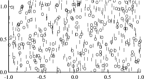
Figure 2: A random distribution of dislocation sources, circles, and dislocation obstacles, lines.

The two-dimensional crystals considered are initially free of mobile dislocations and a random distribution of dislocation sources and a random distribution of dislocation obstacles are specified as illustrated in Fig. 2. A Gaussian distribution dislocation source strengths is specified with a mean Peach-Koehler force for nucleation and an associated standard deviation. Similarly, a Gaussian distribution of dislocation obstacle strengths is specified. The same dislocation mobility constant $B^{K}$ is prescribed for all dislocations.

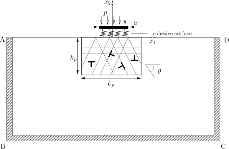
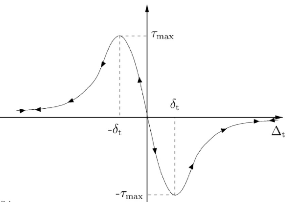
Figure 3: (a) Sketch of the boundary value problem to model the initiation of sliding by Deshpande et al. (2004, 2005). (b) The softening shear cohesive relation used by Deshpande et al. (2004, 2005) .

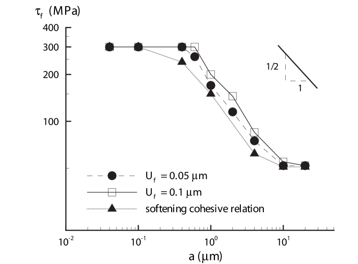
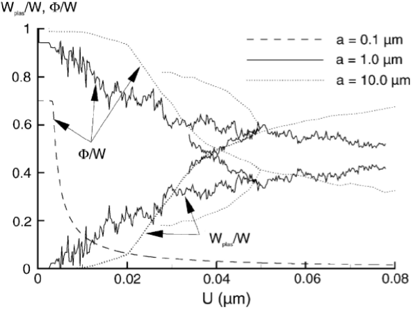
Figure 4: (a)Friction stress as a function of contact size $a$. (b) Plastic dissipation $W_{\rm plas}$, strain energy $\Phi$ and cohesive energy $W_{\rm cohes}$ normalized by the work $W$ as a function of sliding displacement $U$. From Deshpande et al. (2004, 2005)

Deshpande et al. (2004, 2005) carried out calculations modeling the initiation of sliding over asperities of various sizes. The plane strain boundary value problem sketched in Fig. 3a was analyzed. Monotonically increasing displacements were applied on the boundaries AB, BC and CD in the $x_{1}-$direction to give an overall shear displacement $U$ together with a normal pressure of magnitude $p$ over the asperity length $a$. Two types of shear cohesive relations (a cohesive relation specifies the relation between the traction/traction rate across an interface and the displacement/displacement rate jump across it) were used to characterize the interface: (i) a softening cohesive relation, i.e. the shear stress decreases to zero for a sufficiently large relative displacement as shown in Fig. 3b; and (ii) a non-softening relation in which the shear traction reaches a maximum and then remains constant. For the softening cohesive relation, the initiation of sliding was identified with the shear traction reaching zero within a numerical tolerance. For the non-softening cohesive relation the initiation of sliding was identified with attaining a specified value of shear displacement. Also, as sketched in Fig. 3, dislocation activity was restricted to a region around the contact. Calculations were terminated prior to dislocations reaching the boundary of that region.

The definition of the friction stress $\tau_{\rm fr}$ depended on the shear cohesive relation used. For the softening cohesive relation, it was the shear stress just before the shear stress magnitude dropped to zero. For the non-softening cohesive relation, $\tau_{\rm fr}$ was the shear stress at the value of shear displacement $U$ identified as the initiation of sliding. Thus, for the non-softening cohesive relation the value of $\tau_{\rm fr}$ was somewhat arbitrary.

Fig. 4a shows the effect of the contact size $a$ on $\tau_{\rm fr}$. For the non-softening cohesive relation, results are shown using two values of shear displacement $U$ to define the onset of sliding that differ by a factor of two. Regardless of the definition of sliding initiation, the variation of the shear stress at the initiation of sliding, $\tau_{\rm fr}$, with contact size $a$ exhibits two plateaus: for large contacts $\tau_{\rm fr}$ was found to be approximately equal to the tensile yield strength, while for small contacts, it is equal to the cohesive strength, which is $\approx 6$ times larger than the yield strength. In between these two plateaus, $\tau_{\rm fr}$ varies as $\sqrt{a}$.

The evolution of plastic dissipation, i.e. $\int{\cal D}dt$ and denoted by $W_{\rm plas}$ in Deshpande et al. (2004, 2005), elastic energy, $\Phi$, and cohesive energy, $W_{\rm cohes}$ (the energy stored in the cohesive surface), are shown in Fig. 4b for $a=0.1\mu$m (the upper plateau), $1.0\mu$m (the transition region) and $10.0\mu$m (the lower plateau). On the upper plateau, $a=0.1\mu$m , the energy is partitioned into elastic energy $\Phi$ and cohesive energy $W_{\rm cohes}$, with the elastic energy dominating the early stages of sliding and the cohesive energy the latter stages of sliding. On the lower plateau, $a=10.0\mu$m, the partitioning is mainly between $\Phi$ and $W_{\rm plas}$. In between, $a=1.0\mu$m, all three components of the energy are significant. This illustrates the predicted contact size dependence of energy partitioning for the initiation of frictional sliding.

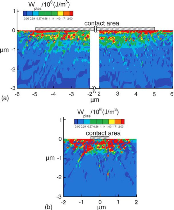
Figure 5: Distribution of the plastic dissipation $w_{\rm plas}$ per unit volume for: (a) contact size $a=10\mu$m and (b) contact size $a=1\mu$m. The contact area is indicated. From Deshpande et al. (2005).

Fig. 5 shows the distribution of plastic dissipation per unit volume, $W_{\rm plas}$, for the $a=1.0\mu$m and $a=10.0\mu$m sizes. For $a=10\mu$m, plastic dissipation mainly occurs near the contact surface but the high dissipation region extends somewhat in front of and behind the contact area. For $a=1.0\mu$, the high dissipation region extends much more deeply into the crystal. Thus, not only the energy partitioning but also the spatial distribution of plastic dissipation is size dependent.

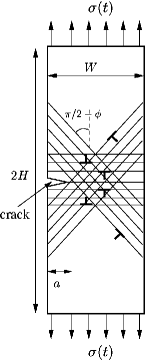
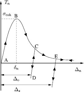
Figure 6: (a) Sketch of the single crystal short crack boundary value problem analyzed by Deshpande et al. (2003a). (b) The cohesive relation used by Deshpande et al. (2003a).

The evolution of dissipation under cyclic loading, i.e. hysteresis, plays a major role in determining the fatigue behavior of materials. It has long been appreciated that short fatigue cracks in metallic components grow faster than long cracks subject to the same cyclic loading range. For sufficiently long cracks, fatigue crack growth is governed by a critical stress intensity factor range (the stress intensity factor $K$ is proportional to $\sigma\sqrt{a}$, where $\sigma$ is the applied stress and $a$ is the crack length), while for sufficiently short cracks, fatigue crack growth is governed by a critical stress range, see e.g. Suresh (1991).

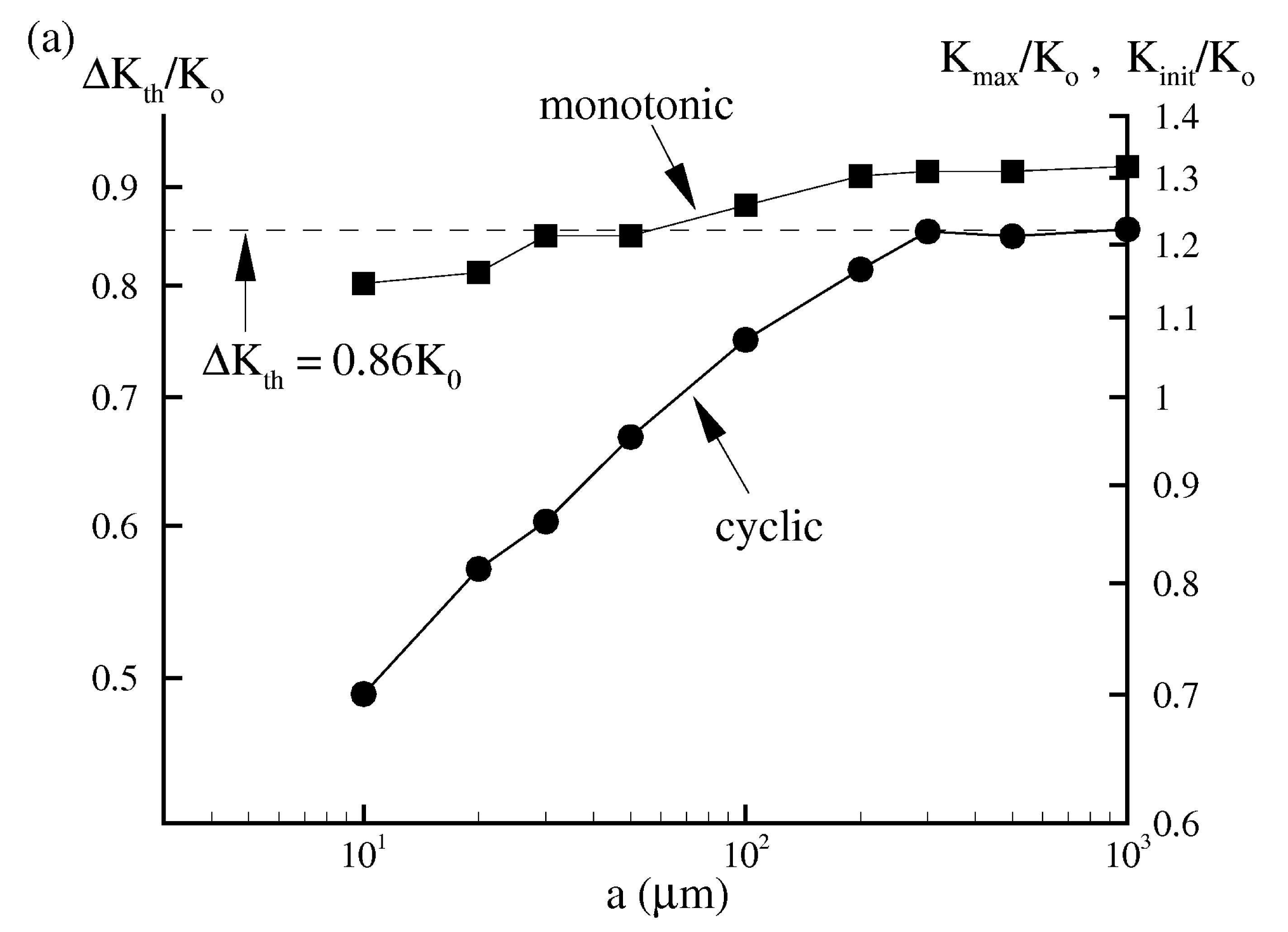
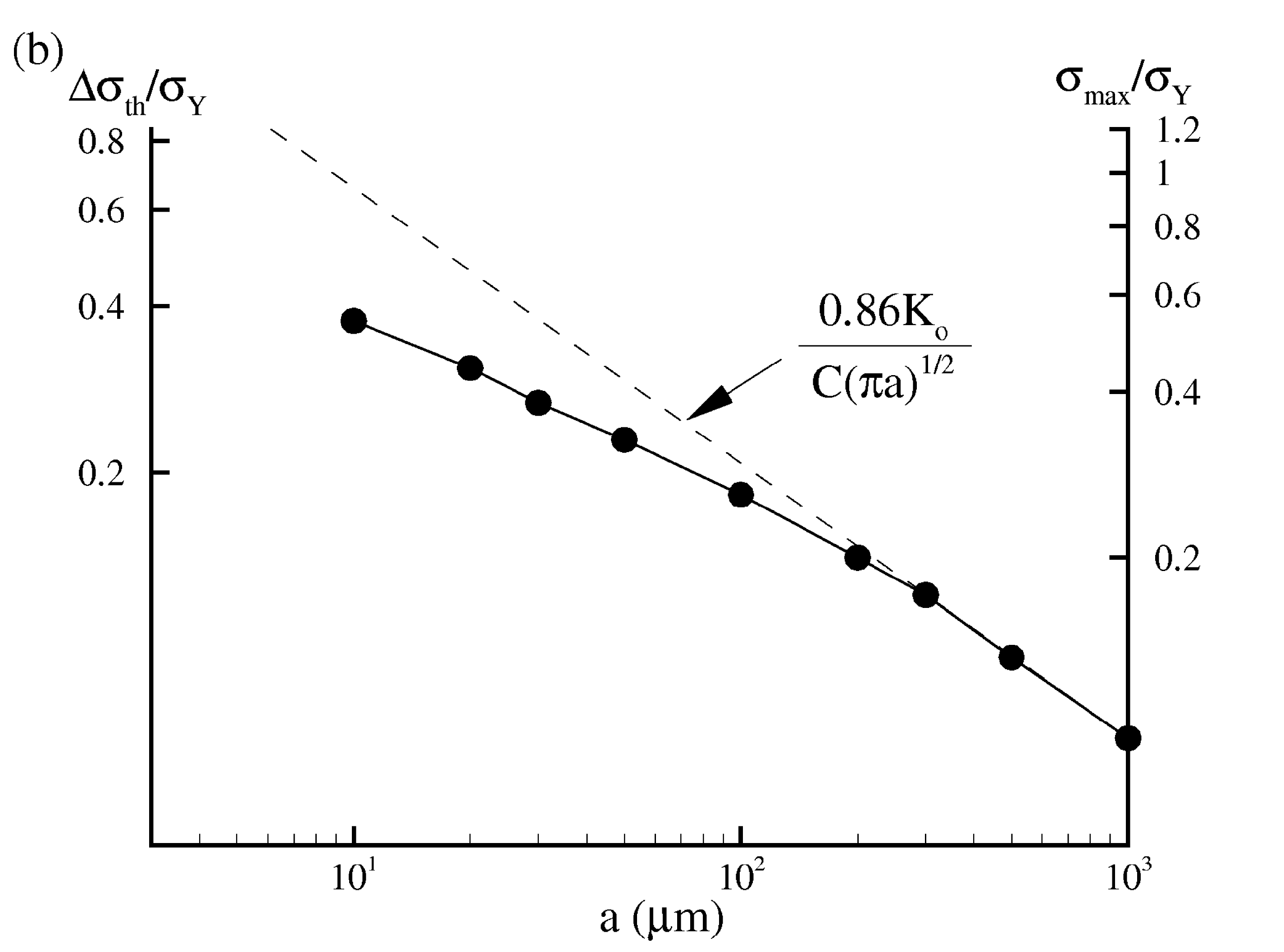
Figure 7: (a) The normalized fatigue threshold $\Delta K_{\rm th}/K_{o}$ versus initial crack length $a$. (b) The normalized fatigue threshold versus crack length $a$ as a function of $\Delta\sigma/\sigma_{y}$ (left axis) and as a function of $\sigma_{\rm max}/\sigma_{y}$ (right axis). The dotted lines show the predictions for $\Delta K$ governed crack growth. From Deshpande et al. (2003a).

Deshpande et al. (2003a) carried out calculations of crack growth for various edge cracked single crystals having the geometry sketched in Fig. 6a (in the calculations of Deshpande et al. (2003a), as in those of Deshpande et al. (2004, 2005) dislocation activity was confined to a region near the crack tip). The presumption underlying the analyses of Deshpande et al. (2003a) is that crack growth is stress driven and that the main source of dissipation is a consequence of the glide of dislocations that nucleate from sources in the crystal. Stress driven crack growth is modeled via the tensile cohesive relation shown in Fig. 6b. Two applied tensile displacement loading histories were considered: (i) displacements that monotonically increase; and (ii) displacements that are a cyclic function of time.

The results of Deshpande et al. (2003a) are summarized in Fig. 7a which shows the dependence of the predicted initiation of crack growth under both monotonic and cyclic loading for geometrically similar specimens as a function of edge crack length $a$. For the edge cracked specimen the relation between the overall stress $\sigma$ and the linear elastic stress intensity factor $K$ is known. For a sufficiently long crack, the linear elastic stress intensity factor acts as the crack driving force and cyclic loading is characterized by $\Delta K=K_{\rm max}-K_{\rm min}$. The fatigue threshold $\Delta K_{\rm th}$ is the smallest value of $\Delta K$ that is found to lead to crack growth (in general $\Delta K_{\rm th}$ depends on the ratio $K_{\rm min}/K_{\rm max}$). Also, the Griffith stress intensity factor, $K_{0}$, is proportional to the square root of the cohesive energy.

For monotonic loading $K_{\rm init}/K_{0}$ is shown (right axis) and for cyclic loading both $\Delta K_{\rm th}/K_{0}$ (left axis) and $K_{\rm max}/K_{0}$ (right axis) are shown. In Fig. 7b the fatigue threshold results for cyclic loading are plotted versus $\Delta\sigma=\sigma_{\rm max}-\sigma_{\rm min}$ and $\sigma_{\rm max}$ showing the transition to stress controlled, rather than stress intensity controlled, crack growth resistance for sufficiently short cracks.

Discrete dislocation plasticity analyses predict that organized dislocation structures that develop in the vicinity of a crack tip can result in crack tip opening stresses approximately an order of magnitude larger than predicted by conventional continuum plasticity, e.g. Cleveringa et al. (2000). These near crack tip organized dislocation structures increase stress levels and hence the associated defect stored elastic energy.

The results of Deshpande et al. (2003a) indicate that the development of the near crack tip stress fields and their associated dissipation depends on both the crack length and whether the loading is monotonic or cyclic. Although both the monotonic and cyclic crack growth results exhibit a decreased resistance to crack growth for sufficiently short cracks, the decline in crack growth resistance for short cracks is much greater under cyclic loading conditions than it is under monotonic loading conditions. For short cracks under cyclic loading conditions, crack growth was found to take place for values of $K_{\rm max}<K_{0}$.

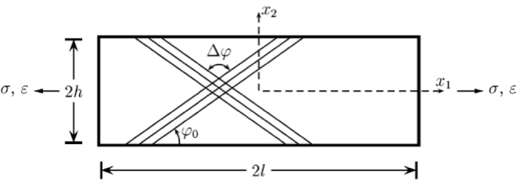
Figure 8: The plane strain single crystal analyzed by Benzerga et al. (2005).

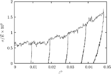
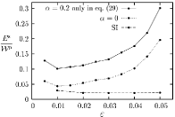
Figure 9: (a) The normalized stress strain curve with unloading showing the predicted Bauschinger effect. (b) Ratio of the stored energy, $E_{s}$, to plastic work, $W_{p}$, versus imposed strain, $\epsilon$. The stored energy $E_{s}$ is defined as the elastic energy $\phi$ minus the elastic energy associated with the overall stress. Also, $\alpha$ is a parameter characterizing the dislocation line tension and SI denotes the response with only static sources and obstacles. From Benzerga et al. (2005).

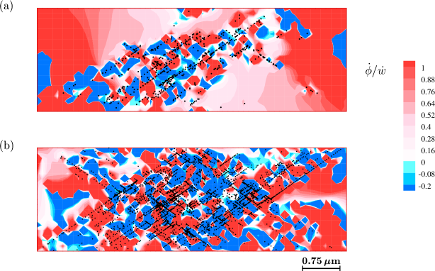
Figure 10: Distributions of the ratio of the local stored energy rate,$\dot{\phi}$, to the local rate of working, $\dot{w}$. (a) $\epsilon=0.01$. (b) $\epsilon=0.04$. From Benzerga et al. (2005).

Knowledge of the partitioning between stored elastic energy and dissipation is needed for predicting the deformation modes that occur in machining and penetration, and for predicting the thermal softening behavior that promotes mechanical instabilities, Furthermore, the stored energy is associated the internal stress state so that there is a direct connection between the energy partitioning and the Bauschinger effect.

Benzerga et al. (2005) calculated the energy partitioning for a single crystal under plane strain tensile loading. Fig. 8 illustrates the plane strain tension specimen analyzed. A major difference between the plane strain tension problem and those modeling sliding and crack growth is that there are no imposed strain gradients for plane strain tension. With no imposed strain gradient, the simple constitutive rules used in those analyses do not give rise to dislocation structures that contribute to the elastic energy. In Benzerga et al. (2005) the two-dimensional discrete dislocation plasticity constitutive rules used to model sliding and crack growth were augmented to account for the effects of line tension, three-dimensional dislocation interactions and, in particular, the dynamic creation of new obstacles and sources as proposed by Benzerga et al. (2003).

One crystal geometry analyzed had slip systems with an initial unsymmetrical orientation relative to the loading axis. Fig. 9 shows results for such a crystal. In Fig. 9a there is a strong Bauschinger effect, the magnitude of which increases with increasing strain. Fig. 9b shows the evolution of the ratio of stored energy $E^{s}$ to plastic work $W^{p}$. The parameter $\alpha$ characterizes line tension with $\alpha=0$ denoting that line tension is not included in the analysis. The result marked SI denotes a calculation with only static sources and obstacles that results in the energy storage being very small $E^{s}/W^{p}<\approx 0.04$, so that nearly all plastic working is dissipated. When the dynamic creation of sources and obstacles is included in the analysis, significantly more elastic energy is stored. The quantity $1-E^{s}/W^{p}$ is the fraction of plastic work dissipated that is used in phenomenological calculations to induce thermal softening. The modeling results in Fig. 9b and the experimental results of Hodowany et al. (2000) indicate that this fraction is not necessarily a constant but can vary with the loading.

Fig. 10 shows the distribution of the rate of energy storage,$\dot{\phi}/\dot{w}$, and the dislocation positions at two values of overall strain $\epsilon$. In regions that remain essentially elastic, $\dot{\phi}/\dot{w}\approx 1$, as expected. In regions with a high dislocation density this ratio has peak values much larger than the overall ratio, $\dot{\Phi}/\dot{W}$ showing that local values of the energy storage rate can differ significantly from the overall global value.

A beginning of the emergence of organized dislocation structures can be seen in Fig. 10. Such organized dislocation structures affect the internal stress field and, hence, the energy partitioning. Without a strong applied stress/strain gradient to drive the dislocation structure formation, the details of dislocation interactions dominate. Most likely, a full three-dimensional discrete dislocation plasticity analysis is needed to provide an accurate picture of their development. However, such dislocation structures develop at moderate to large deformations and nearly all discrete dislocation plasticity analyses have been based on small deformation kinematics which, among other limitations, cannot reasonably account for the effects of lattice rotations. Finite deformation formulations are available, Deshpande et al. (2003b); Irani et al. (2015), but use has been very limited.

For both the Bauschinger effect in Fig. 9a and the short crack effect in Fig. 7, a key role is played by the evolution of the discrete dislocation structure under reverse loading in the heterogeneous internal stress state induced by the discrete dislocation structure that develops under forward loading. Indeed, the release of stored elastic energy associated with such a stress state plays a key role in driving fatigue crack growth with $K_{\rm max}<K_{0}$.

5 Discrete STZ plasticity

Plastic deformation in a variety of amorphous solids occurs via discrete regions of atomic rearrangement called shear transformation zones (STZs), Argon (1979); Spaepen (1977) and the representation of STZs in terms of transforming Eshelby (1957, 1959) inclusions was pioneered by Bulatov and Argon (1994).

A transforming Eshelby (1957, 1959) inclusion is an ellipsoidal sub-volume of a uniform linear elastic solid undergoes a stress-free transformation, i.e. if the transforming inclusion had been removed from the matrix, it would have undergone a uniform strain with zero stress. Since the inclusion was not free to deform, it and the surrounding matrix are stressed. For an ellipsoidal inclusion, the strain and stress fields inside the inclusion associated with the constrained transformation are also uniform. Due to the displacement field associated with the transformation there is a displacement jump across the inclusion/matrix interface. In general, the transformation reduces the stress level inside the inclusion and induces a stress concentration outside the inclusion.

Transforming Eshelby (1957, 1959) inclusions are used to model a wide variety of phenomena in addition to STZs including, for example, phase transformations and internal stress states in heterogeneous materials. For discrete STZ plasticity, the location and size of an STZ is fixed, and the transformation strain evolves. Also, for discrete STZ plasticity, the stress field outside the inclusion varies as $1/r^{2}$ (2D) or $1/r^{3}$ (3D) which gives a much more rapid stress decay than the $1/r$ variation for dislocations. Other applications, for example the modeling of some phase transformations, may involve Eshelby (1957, 1959) inclusions with a size that varies with time and with either a fixed or evolving transformation strain. Although the focus here is on shear transformations, the general results regarding dissipation rate apply to fixed-size Eshelby (1957, 1959) inclusions with general transformation strains.

5.1 Dissipation rate for discrete STZ plasticity

In discrete STZ plasticity modeling, $dS$ in Eq. (28) is fixed and the displacement rate jump evolves. With the transformation strain rate of inclusion $K$ denoted by $\dot{\epsilon}^{*K}_{ij}$, the displacement rate jump across interface $K$ is $\Delta\dot{u}^{K}_{i}=\dot{\epsilon}^{*K}_{im}x_{m}$ in Eq. (28) so that

$$\dot{\cal D}=\sum_{K=1}^{N}\int_{S^{K}}\sigma^{K}_{ij}n_{j}\dot{\epsilon}^{*K}_{im}x_{m}dS$$ (37)

or changing to a volume integral for an Eshelby (1957, 1959) inclusion

$$\dot{\cal D}=\sum_{K=1}^{N}\left[\int_{V^{K}}\sigma^{K}_{ij}dV\right]\dot{\epsilon}^{*K}_{ij}+\sum_{K=1}^{N}\left[\int_{V^{K}}\sigma^{K}_{ij,j}x_{m}dV\right]\dot{\epsilon}^{*K}_{im}$$ (38)

and because $\sigma^{K}_{ij,j}=0$

$$\dot{\cal D}=\sum_{K=1}^{N}\left[\int_{V^{K}}\left(\hat{\sigma}_{ij}+\sum_{M=1}^{N}\sigma^{T_{M}}_{ij}\right)dV\right]\dot{\epsilon}^{*K}_{ij}=\sum_{K=1}^{N}Z^{K}_{ij}\dot{\epsilon}^{*K}_{ij}$$ (39)

where $\sigma^{T_{M}}_{ij}$ is the transformation stress of inclusion $M$ and $Z^{K}_{ij}$ is the configurational force type quantity conjugate to $\dot{\epsilon}^{*K}_{ij}$ given by

$$Z^{K}_{ij}=\int_{V^{K}}\left(\hat{\sigma}_{ij}+\sum_{M=1}^{N}\sigma^{T_{M}}_{ij}\right)dV$$ (40)

Direct calculations of dissipation and dissipation rate for Eshelby (1957, 1959) inclusions have been given by Vasoya et al. (2019, 2020).

Defining an average stress quantity in inclusion $K$ by

$$\bar{\sigma}^{K}_{ij}=\frac{1}{V^{K}}\int_{V^{K}}\sigma_{ij}^{K}dV$$ (41)

Eq. (40) can be written as

$$Z^{K}_{ij}=\left(\bar{\hat{\sigma}}_{ij}+\sum_{M\neq K}\bar{\sigma}^{T_{M}}_{ij}+\sigma^{T_{K}}_{ij}\right)V^{K}$$ (42)

since $\sigma^{T_{K}}_{ij}$ is uniform in $V^{K}$. Also, if the inclusion size is sufficiently small compared to the distance over which $\hat{\sigma}_{ij}$ and $\sigma^{T_{M}}_{ij}$ vary, the average values in Eq. (42) can be well-approximated by their values at the inclusion center.

Focusing attention on Eshelby (1957, 1959) inclusion $K$, a non-negative dissipation rate is guaranteed by a linear relation of the form

$$\dot{\epsilon}^{*K}_{ij}={\cal K}^{K}_{ijkl}Z_{kl}^{K}$$ (43)

where $Z_{kl}^{K}$ is given by Eq. (40) and the tensor ${\cal K}^{K}_{ijkl}$ is positive semi-definite, i.e. satisfies $B_{ij}{\cal K}^{K}_{ijkl}B_{kl}\geq 0$ for any second order tensor ${\bf B}$.

For an isotropic relation in Eq. (43), ${\cal K}^{K}_{ijkl}$ has the form

$${\cal K}^{K}_{ijkl}=\frac{1}{2}\kappa^{K}_{1}\left(\delta_{ik}\delta_{jl}+\delta_{il}\delta_{jk}\right)+\kappa^{K}_{2}\delta_{ij}\delta_{kl}$$ (44)

so that

$$\dot{\epsilon}^{*K}_{ij}=\kappa^{K}_{1}Z^{K}_{ij}+\kappa^{K}_{2}Z^{K}_{kk}\delta_{ij}$$ (45)

where $\delta_{ij}$ is the Kronecker delta.

The dissipation rate in inclusion $K$ can now be written as

$$\dot{\cal D}^{K}=Z^{K}_{ij}\dot{\epsilon}^{*K}_{ij}=\kappa^{K}_{1}Z^{K}_{ij}Z^{K}_{ij}+\kappa^{K}_{2}\left(Z^{K}_{kk}\right)^{2}\geq 0$$ (46)

and the total dissipation rate is

$$\dot{\cal D}=\sum_{K}\dot{\cal D}^{K}$$ (47)

Non-negative $\dot{\cal D}$ does not require each $\dot{\cal D}^{K}$ to be non-negative. If one $\dot{\cal D}^{K}$ is negative, the dissipation rate in a sub-volume including only that inclusion is negative so that the Coleman-Noll postulate (Coleman and Noll, 1964) is then not satisfied.

5.1.1 Plane strain shear transformation

As an illustration of the general expressions, the relations for plane strain shear of a circular inclusion are presented as used, for example, in the numerical STZ calculations of Vasoya et al. (2020, 2021). In the numerical calculations, it is assumed that the STZ is sufficiently small relative to the length scale over which stresses vary so that the stress state in the STZ can be regarded as uniform.

With the transformation strain in STZ $K$ being $\gamma^{*K}(s_{i}n_{j}+s_{j}n_{i})/2$, where $s_{i}$ gives the shear direction and $n_{i}$ is normal to $s_{i}$, $Z^{K}_{sn}$ is given by (Vasoya et al., 2020)

$$Z^{K}_{sn}=\frac{E}{2(1-\nu^{2})}\left[\frac{4{\sigma}^{K}_{sn}(1-\nu^{2})}{E}-\gamma^{*K}\right]A^{K}_{\rm incl}$$ (48)

where $A^{K}_{\rm incl}$ is the inclusion area.

The dissipation rate associated with the transformation of STZ $K$ is $\dot{{\cal D}}^{K}=Z^{K}_{sn}\dot{\gamma}^{*K}$ and with the kinetic relation for $\gamma^{*K}$ taken as

$$\dot{\gamma}^{*K}=\frac{1}{B^{K}}\left[\frac{1}{A_{\rm incl}}\frac{2(1-\nu^{2})Z^{K}_{sn}}{E}\right]=\frac{1}{B^{K}}\left[\gamma^{*K}_{\rm max}-\gamma^{*K}\right]$$ (49)

where

$$\gamma^{*K}_{\rm max}=\frac{4{\sigma}^{K}_{sn}(1-\nu^{2})}{E}$$ (50)

The dissipation rate is given by

$$\dot{{\cal D}}^{K}=\frac{1}{B^{K}}\left(\frac{EA_{\rm incl}}{2(1-\nu^{2})}\right)\left(\gamma^{*K}_{\rm max}-\gamma^{*K}\right)^{2}$$ (51)

and is guaranteed to be non-negative.

From Eq. (50), $\gamma^{*K}_{\rm max}$ is of the order of the STZ stress divided by an elastic modulus. Quite generally, the limiting strain magnitude for a non-negative dissipation rate or even non-negative total dissipation is of the order of the Eshelby (1957, 1959) inclusion stress level divided by a relevant elastic modulus, Vasoya et al. (2019).

Composition	E (GPa)	$\nu$	$\sigma_{y}$ (GPa)	Vol. $\dot{\cal D}\geq 0$	Shear $\dot{\cal D}\geq 0$
Nd60Al10Fe20Co10	51.0	0.342	0.45	0.00295	0.0128
Ho55Al25Co20	67.0	0.34	0.87	0.0043	0.0188
Zr48Be24Cu12Fe8Nb8	95.7	0.359	1.6	0.0054	0.0242
Zr46Cu46Al8	96.0	0.37	1.67	0.0055	0.0253
Fe50Cr15Mo14C15B6	217.0	0.323	4.17	0.0065	0.0277
Ti45Zr20Be35	96.8	0.356	1.86	0.0062	0.0279
Cu50Hf43Al7	113.0	0.345	2.2	0.0064	0.0281
Zr52.5Cu17.9Ni14.6Al10Ti5	88.4	0.374	1.91	0.0068	0.0324
Ca65Li9.96Mg8.54Zn16.5	23.0	0.277	0.53	0.0083	0.0329

Table 1: Condensed version of the table of Vasoya et al. (2019) showing the limiting transformation strains for a single transforming inclusion to have a non-negative dissipation rate with a uniform remote stress. The values of $E$, $\nu$ and $\sigma_{y}$ are taken from Qu et al. (2015).

The data in Table 1 is taken from Vasoya et al. (2019) and shows the limiting transformation strains for a non-negative dissipation rate for a shear transformation and for a volumetric transformation with the transformation stress taken to correspond to the macroscopic stress at the onset of plastic yielding. The limiting transformation strain magnitudes for a non-negative dissipation rate are all less than $0.035$. Atomistic calculations, Dasgupta et al. (2013); Albert et al. (2016), and experiments, Argon and Shi (1983); Hufnagel et al. (2016), are, when interpreted in terms of a transforming Eshelby (1957, 1959) inclusion, consistent with transformation strains $\gamma^{*K}$ that are greater than $\gamma^{*K}_{\rm max}$.

There are several possible reasons for the discrepancy between the limiting strain values in Table 1 and the atomistic calculations and experiment. The limiting values of transformation strain in Table 1 were calculated assuming linear elasticity and identifying the stress at transformation with the yield strength. Local stress concentrations would increase the stress magnitude at the nucleation site and thus lead to an increased allowable transformation strain. It could be necessary to account for entropy, either temperature related entropy or configurational related entropy, as in a continuum STZ plasticity formulation, Bouchbinder and Langer (2009); Falk and Langer (2011).

One possibility, considered by Vasoya et al. (2020), is that the term $\Theta\dot{s}$ in Eq. (6) associated with a transformation is sufficiently positive for the Clausius-Duhem inequality to be satisfied even if the mechanical dissipation is negative. Another possible consequence of accounting for the entropy increase associated with the transformation is having different elastic moduli in the STZ ((through the entropy dependence of the energy $\phi$) from those in the material outside. The results of Vasoya et al. (2019) for a single transforming STZ in an infinite isotropic elastic solid with a uniform applied stress $\sigma_{ij}^{0}$ at infinity can give a qualitative indication of the effect.

For a plane strain shear transformation of a circular STZ with a mismatch in Young’s modulus $E$ between the material inside the STZ and that outside the STZ, but with the same value of Poisson’s ratio $\nu$ inside and outside the STZ, the ratio of mismatch/uniform values of the maximum transformation shear strain for non-negative dissipation/dissipation rate at the same value of $\sigma^{(0)}_{12}/G^{\rm out}$, $R_{\rm mism}$, calculated from Eq. (70) of Vasoya et al. (2019), is

$$R_{\rm mism}=\frac{\gamma^{*}_{\rm mism}}{\gamma^{*}_{\rm unif}}=\frac{G^{\rm out}/G^{\rm in}+(3-4\nu)}{1+(3-4\nu)}$$ (52)

where $G=E/2(1+\nu)$ and $(\ )^{\rm in}$ and $(\ )^{\rm out}$ denote values inside and outside the STZ, respectively. For $R_{\rm mism}$ in Eq. (52) to be greater than $1$, $G^{\rm in}<G^{\rm out}$, so that the effect of entropy needs to be to reduce the stiffness in the STZ. For example, with $\nu=0.325$, $R_{\rm mism}=2$ for $G^{\rm in}/G^{\rm out}=0.269$ and $R_{\rm mism}=3$ for $G^{\rm in}/G^{\rm out}=0.156$. This suggests that in order to increase the transformation strain for a non-negative dissipation rate by a factor of $2$ to $3$, this entropy contribution would need to substantially reduce the stiffness inside the STZ, by a factor of $\approx 4-6$ in this simple estimate.

Another possibility, focused on here, is that the transformation strain magnitude for some transformations exceeds that required for a non-negative dissipation rate. If this occurs, requiring a non-negative dissipation rate (i.e. satisfaction of the Clausius-Duhem inequality) for all points of the body and for all time is an overly restrictive requirement. For a limiting transformation strain $\gamma^{*K}_{\rm non}>\gamma^{*K}_{\rm max}$, an evolution equation analogous to Eq. (49) is

$$\dot{\gamma}^{*K}=\frac{1}{B^{K}}\left[\gamma^{*K}_{\rm non}-\gamma^{*K}\right]$$ (53)

with the dissipation rate, $\dot{{\cal D}}^{K}$, given by

$$\dot{{\cal D}}^{K}=\frac{1}{B^{K}}\left(\frac{EA_{\rm incl}}{2(1-\nu^{2})}\right)\left(\gamma^{*K}_{\rm max}-\gamma^{*K}\right)\left(\gamma^{*K}_{\rm non}-\gamma^{*K}\right)$$ (54)

$\dot{{\cal D}}^{K}$, is negative for $B^{K}>0$ and $\gamma^{*K}>\gamma^{*K}_{\rm max}$.

The possibility of a negative dissipation rate can be understood by focusing attention on a sub-volume containing only STZ $K$ and noting that the rate form of conservation of energy requires $\dot{W}=\dot{\Phi}+\dot{\cal{D}}^{K}$ for that sub-volume. The transformation reduces stress levels in the STZ and increases stress levels outside the STZ so that $\dot{\Phi}$ outside the STZ increases. If the total $\dot{\Phi}=\dot{\Phi}_{\rm in}+\dot{\Phi}_{\rm out}$, which increases with increasing transformation strain, is sufficiently large the rate form of conservation of energy can require $\dot{\cal{D}}^{K}<0$.

5.2 Calculations of discrete STZ plasticity dissipation

There are few solutions of STZ plasticity boundary value problems compared with those for discrete dislocation plasticity, particularly solutions based on transformation strain relations that guarantee a non-negative dissipation rate. In their work on developing STZ evolution relations that guarantee a non-negative dissipation rate, Vasoya et al. (2020) presented some results for the plane strain tension problem illustrated in Fig. 8 (but of course with no slip planes).

An initial distribution of potential STZ sites is specified with each site having a specified critical shear strain energy for activation taken from a Gaussian distribution. Also, each potential STZ site is taken to be circular with the evolution of its transformation shear strain as given in Eq. (49).

In the calculations of Vasoya et al. (2020), $B^{K}=B$ for all STZs and the direction of shear when as STZ is activated is taken to be a maximum shear direction at the STZ center. The boundary value problem is solved using the superposition formulation in Section 3.1. An advantage of this formulation is that the STZ size can be much smaller than the finite element size used to solve for the $(\hat{\ })$ fields so that there can be many STZs per finite element.

For a non-negative dissipation rate, the transformation strain magnitude is limited to $\gamma^{*K}_{\rm max}$, which is typically in the range $0.03$ to $0.04$, but plastic strains larger than $\gamma^{*K}_{\rm max}$ are observed in metallic glass shear bands, e.g. Mass and Löffler (2015). Obtaining larger shear strains with a non-negative dissipation rate requires STZs to be able to activate more than once. A time parameter $t_{D}$ is introduced so that reactivation can only occur after a delay of $t_{D}$ from the previous activation. Thus, even though each activation is constrained to have a transformation strain sufficiently small to be associated with a non-negative dissipation rate, repeated reactivation permits larger transformation strains to accumulate in an STZ. Also, in order to provide the possibility of plastic deformation occurring between the initial potential STZ sites, when an STZ site activates, new potential STZ activation sites can nucleate in the vicinity of an activated site.

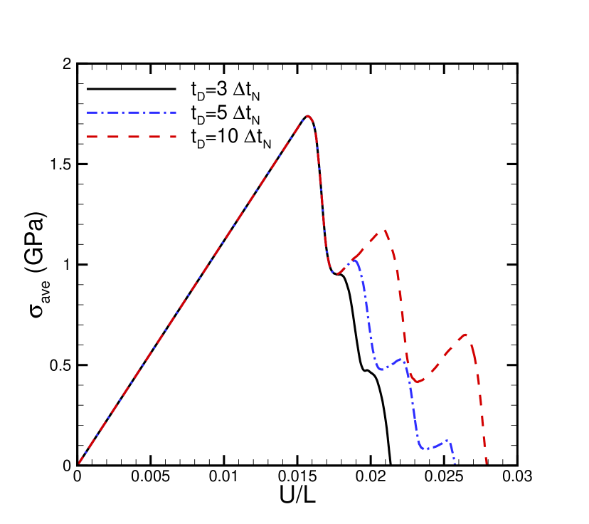
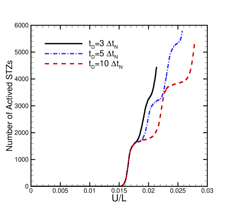
Figure 11: The dependence of the stress-strain response and the evolution of STZs on the delay time for reactivation $t_{D}$ with $B=0.001$ s. (a) Stress-strain curves. (b) Evolution of the number of activated STZs with overall strain, $U/L$. From Vasoya et al. (2020).

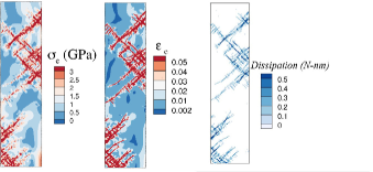
(a)                        (b)                          (c)

Figure 12: Distributions of (a) Effective stress, $\sigma_{e}$. (b) Effective strain, $\epsilon_{e}$. (c) Energy dissipation. Unpublished results based on the work of Vasoya et al. (2020).

To illustrate the sort of responses that are obtained when implementing the STZ kinetic relation in a numerical calculation of STZ plasticity, results are shown for three values of the reactivation time $t_{D}$, with fixed $B$, and for two values of $B$, with fixed reactivation time $t_{D}$ in Fig. 11. In Fig. 11a computed stress-strain curves are shown with $\sigma_{\rm ave}$ is the average stress on $x_{2}=L$ (where $U(t)$ is prescribed). As the reactivation time decreases, the load drops more rapidly. Fig. 11b shows the evolution of the number of activated STZ sites. Bursts of STZ activation occur with the bursts associated with the drops in $\sigma_{\rm ave}$ in Fig.  11a. The strain interval between bursts of activation increases with increasing $t_{D}$. For $t_{D}=5\Delta t_{N}$ and $10\Delta t_{N}$ there is a clear increase in $\sigma_{\rm ave}$ between the drops, whereas for $t_{D}=3\Delta t_{N}$, the activation bursts occur so close together that the value of $\sigma_{\rm ave}$ does not increase between them.

Fig. 12 shows distributions of effective stress, $\sigma_{e}=\sqrt{3\sigma^{\prime}_{ij}\sigma^{\prime}_{ij}/2}$, where $\sigma^{\prime}_{ij}$ is the stress deviator $\sigma^{\prime}_{ij}=\sigma_{ij}-\sigma_{kk}\delta_{ij}/3$, Fig. 12a, the corresponding effective strain $\epsilon_{e}$, Fig. 12b, and plastic dissipation, Fig. 12c. Because most of the deformation arises from the STZ transformation strain and since there can be multiple active STZ sites per finite element, plotting field values on the finite element mesh gives averages over that element which masks details of the distributions. The distributions shown were obtained on a grid having a mesh spacing about $1/8$ the finite element spacing which allows a better representation of the spatial variation of the $(\tilde{\ })$ fields. The regions with elevated effective stress, strain and dissipation correspond to regions of intense STZ activity. Local values of $\sigma_{e}$ could approach $E/10$. Thus, for discrete STZ plasticity regions of large local dissipation do not necessarily significantly reduce stress levels.

Although, the numerical results in Kondori et al. (2018); Vasoya et al. (2020) show that strains larger than the transformation strain can be reached in a shear band by repeated reactivation, they do not resolve the discrepancy between the transformation strains associated with atomistic calculations and experiment for a single transformation and the limiting strain predicted from requiring an Eshelby (1957, 1959) transformation to have a non-negative dissipation rate.

6 Size dependence and dissipation in constrained shear

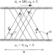
Figure 13: Illustration of the discrete dislocation plasticity problem formulation and boundary conditions for shear of a constrained layer of thickness $H$. From Shu et al. (2001).

Quasi-static simple shear of a constrained strip provides a simple context to investigate the size dependence implications of proposed plastic material characterizations. Length scale independent continuum plasticity predicts a state of uniform shear stress and uniform shear strain that is size independent. Discrete defect characterizations of plastic response inevitably contain one or more length scale dependent material parameters, such as defect size or defect spacing. However, the material characterization containing a length scale does not necessarily result in the overall stress-strain response being size dependent over some range of sizes of interest. In addition, it turns out that whether or not the stress-strain response exhibits size dependence can have implications for the predicted energy dissipation. To illustrate this, results from Shu et al. (2001) and Vasoya et al. (2021) are presented. Much of the focus in Shu et al. (2001) and Vasoya et al. (2021) was on the size dependence of the stress-strain response but here the main aim in presenting their results is to illustrate the implications of the mode of defect evolution for the size dependence of dissipation.

Fig. 13 illustrates the plane strain constrained shear boundary value problem. Simple shear of a strip, of height $H$ was analyzed with an imposed shear displacement $U(t)$. The strip was taken to be unbounded in the directions orthogonal to the height direction. The analyses were carried out in a small deformation framework for plane strain and quasi-static loading conditions.

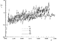
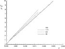
Figure 14: (a) Normalized overall shear stress versus applied shear strain with double slip and various values of $H/d$. (b) Normalized overall shear stress versus applied shear strain with double slip and various values of $H/d$. From Shu et al. (2001)

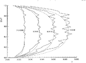
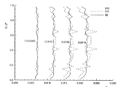
Figure 15: (a) Shear strain profiles at various values of overall shear strain $\Gamma$ for double slip with $H/d=80$ (b) Shear strain profiles at various values of overall shear strain $\Gamma$ for single slip with $H/d=2.3$ and $H/d=80$. From Shu et al. (2001).

Shu et al. (2001) considered planar crystals with two symmetrically oriented slip systems as illustrated in Fig. 13 and cases where dislocation sources (and therefore dislocations) were only present on one system. The crystals analyzed had a specified density of initial dislocation sources with a Gaussian distribution of source strengths and had a specified mobility $B^{K}=B$. Fig. 14 shows the computed overall shear stress versus shear strain responses for the double slip, Fig. 14a, and single slip, Fig. 14b, cases. For double slip, there is significant size dependence and the overall slope of the shear stress versus shear strain curve in the plastic range is much less than the elastic shear modulus. It can also be seen in Fig. 14a that for double slip, presuming nearly elastic unloading, there is significant plastic dissipation. For single slip, Fig. 14b, the slope of the stress strain curve is little reduced from that associated with the elastic shear modulus, very high stress levels are attained at relatively small strains and unloading would reveal little plastic dissipation.

Fig. 15 shows strain profiles in the strip at various values of overall shear strain, $\Gamma$, for double slip, Fig. 15a, and for single slip, Fig. 15b. For double slip, there is a clear boundary layer effect where there is little, if any, shear strain and the shear strain is largest in the center of the strip. For single slip, the shear strain is nearly uniform across the strip as expected for a material with essentially size independent shear stress versus shear strain response as in Fig. 16b.

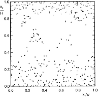
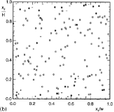
Figure 16: (a) Dislocation distributions in a unit cell with double slip and $H/d=80$. (b Dislocation distributions in a unit cell with single slip and $H/d=80$. From Shu et al. (2001).

The dislocation distributions at one stage of imposed shear are shown in Fig. 16, for a double slip calculation, Fig.  16a, and for a single slip calculation, Fig. 16b. In Fig. 16a, the center of the strip, where the shear strain is maximum in Fig. 15a, is nearly dislocation free while the edges of the strip, where there is little shear strain, have the largest accumulation of dislocations. This is because plastic straining by dislocation glide is associated with where the dislocations used to be as well as with where they are. For the single slip case in Fig. 16b, the distribution of dislocations is fairly uniform in the strip due to limited dislocation glide, giving rise to the rather uniform strain profiles in Fig. 15b.

These results illustrate the implication for size dependence of two possible ways to create plastic strain in discrete dislocation plasticity: (i) nucleate dislocations that glide; and (ii) nucleate dislocations that do not glide (or glide very little).

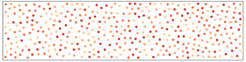
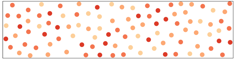
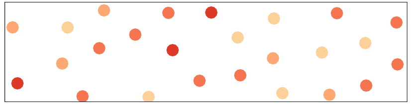
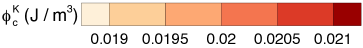
Figure 17: Spatial distribution of the initial potential STZ sites for $L/h=4$. The shading indicates the value of the critical value of shear strain energy density for STZ activation, $\phi_{c}^{K}$, associated with a given site. From Vasoya et al. (2021).

Vasoya et al. (2021) analyzed the same constrained shear problem as illustrated in Fig. 13 (but, of course, with no slip planes) for various shear layer thicknesses (denoted by $h$ in Vasoya et al. (2021)) as pictured in Fig. 17. The strip analyzed is unbounded in the shear direction and consists of a periodic cells of length $L$. The configurations shown in Fig. 17 all have $L/h=4$. There is an initial distribution of circular potential STZ activation sites. Each site is associated with a critical value of strain energy for activation taken from a Gaussian distribution about a specified mean value. Once activated, the shear strain evolves via Eq. (49) so that the dissipation rate associated with the evolution of each STZ is non-negative. Once an STZ activates it can nucleate additional potential STZ sites as described by Vasoya et al. (2021).

Fig. 17 shows plots of the distribution of the initial potential STZ sites. The shading reflects the value of the shear strain energy density for STZ activation, $\phi_{c}^{K}$, associated with a given site. The initial locations of the STZ centers were placed randomly. In order to exclude the possibility of partial STZs at the region boundaries, an exclusion zone that is free of STZ centers, is introduced at each boundary that has the width of one STZ diameter.

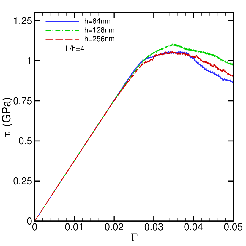
Figure 18: Evolution of shear stress $\tau$ and with overall shear strain $\Gamma$ for $L/h=4$ and and for various values of $h$. From Vasoya et al. (2021).

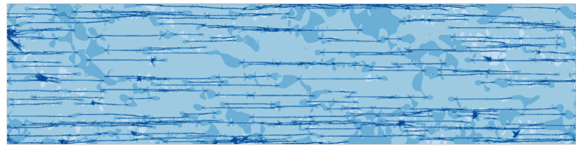
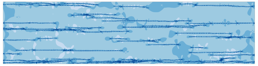
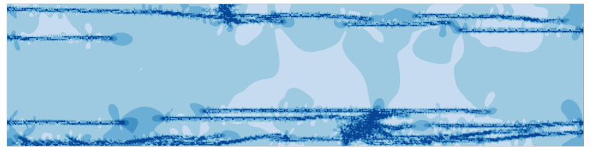
Figure 19: Distribution of effective stress $\sigma_{e}$ at $\Gamma=0.05$ for $L/h=4$. (a) $L=256$nm. (b) $L=128$nm. (c) $L=64$nm. From Vasoya et al. (2021).

Vasoya et al. (2021) analyzed two distributions of activation energies. One was a relatively narrow distribution and the other a relatively broad distribution of activation energies. The results depend on the breadth of the distribution. Here, Figs. 18 and 19 show some results for the relatively broad distribution.

Plots of the calculated overall shear stress versus shear strain responses for several values of layer thickness $H$ are shown in Fig. 18. There is relatively little size dependence, within the range of what is expected for statistical variations, and smaller is not harder. However, the response is very different from the discrete dislocation response response in Fig. 16b where very large overall shear stress magnitudes (relative to the initial flow strength) are reached.

The distributions of Mises effective stress in Fig. 19 show that plastic deformation takes place is well defined shear bands. The development of shear bands is consistent with the softening response in Fig. 18. It is worth noting that very large stress magnitudes, i.e. a significant fraction of the shear modulus, occur in the shear bands.

With the kinetic relation used by Vasoya et al. (2021) which allows for nucleation of new STZ sites, the STZ response is in some ways intermediate between the two discrete dislocation cases of Shu et al. (2001). The STZs do not move through the material as do gliding dislocations but the ability to nucleate new potential STZ sites leads to a percolation-type extension of plastic deformation into new material locations. This leads to a reduction in overall stress as for gliding dislocations but there is relatively little size dependence as for the calculations with dislocations that do not move or move very little.

Although the dissipation rate was not explicitly calculated in the results shown here, it is evident from the overall stress-strain responses that the effect of size on dissipation is different in each case. Fig. 15a is a case where defects move relatively long distances and there is significant plastic dissipation and a size effect, Fig. 15b is a case where defects are stationary and nucleation sites are fixed leading to little plastic dissipation and essentially no size effect, and Fig. 18 is a case where defects do not move but there is a percolation-like nucleation of new defect sources leading to significant plastic dissipation but no significant size effect.

7 Continuum mechanics and a negative dissipation rate

Violation of the Clausius-Duhem inequality over a small region and for a short time has been seen in atomistic simulations, for example Ayton et al. (2001), in macro scale discrete particle simulations of a granular solid (Ostoja-Starzewski and Laudani, 2020), and in experiment, for example Wang et al. (2010). In this regard it is worth noting that molecular dynamics calculations involve an adjustable length scale parameter, typically the particle spacing. While that spacing is regarded as an atomic spacing that is set to be of the order of Angstroms and all other material quantities have a length scale that is relative to that set value. The qualitative features that emerge from the molecular dynamics calculations would hold if the length scale were identified with a larger length scale, of the order of meters or kilometers. Indeed, the analyses of Ostoja-Starzewski and Laudani (2020) were for two-dimensional Couette flow of continuum scale elastic particles interacting via a Hookean contact relation and illustrate that a local violation of the Clausius-Duhem inequality can be associated with discrete events regardless of absolute size.

The extent, if any, to which a local violation of the Clausius-Duhem inequality is relevant for discrete defect plasticity remains to be determined. However, discrete defects events such as STZ activation, phase transformation, etc. can involve relatively few discrete entities, take place over relatively short times and can be influenced by fluctuations. In this context, “large” and “small” are reasonably associated with the number of discrete entities involved in a discrete defect plasticity event. What is a “long time” and what is a “short time” are not so clear.

Typically, in formulating continuum constitutive relations, the form and parameters of a constitutive relation are chosen to satisfy the Coleman-Noll postulate (Coleman and Noll, 1964) so that the Clausius-Duhem inequality is satisfied for all regions of a body and for all time. In Section 7.1 we explore, in a simple one-dimensional continuum mechanics context, the consequences of violating the Coleman-Noll postulate (Coleman and Noll, 1964), i.e. in a purely mechanical framework having a local negative dissipation rate over a small region and for a small time. Note that even if there is justification in some circumstances for adding a sufficiently positive $\dot{s}\Theta$ term so that the Clausius-Duhem inequality is satisfied at each point, the challenge of carrying out a stable mechanical calculation with a negative dissipation rate remains.

7.1 One-dimensional model with a negative dissipation rate

Although the focus of the discrete defect framework is on quasi-static deformations, the consequence of violating the Clausius-Duhem inequality (in the sense of having a negative dissipation rate) over a small region and for a short time is explored in a one-dimensional wave propagation analysis because dynamics provides a simple way to introduce a length scale and a time scale. The non-dimensional interval $0\leq x\leq 1$ is considered with

$$\frac{\partial\sigma}{\partial x}=\rho\frac{\partial^{2}u}{\partial t^{2}}$$ (55)

with the boundary conditions

$$\dot{u}(0)=V(t)\qquad\dot{u}(1)=0$$ (56)

The elastic-viscoplastic constitutive relation is

$$\dot{\sigma}=E(\dot{\epsilon}-\dot{\epsilon}^{p})$$ (57)

where

$$\dot{\epsilon}=\frac{\partial\dot{u}}{\partial x}$$ (58)

and the plastic strain rate is given by

$$\dot{\epsilon}^{p}=\dot{a}\left(\frac{|\sigma|}{\sigma_{0}}\right)^{m}{\rm sign}(\sigma)$$ (59)

The calculations are carried out using non-dimensional material parameters with $E=1$, $\rho=1$, $\sigma_{0}=0.002$ and $m=0.10$.

The imposed tensile velocity is

$$V(t)=\begin{cases}-V_{0}\,t/t_{\rm rise},&\mbox{for }t\leq t_{\rm rise}\\ -V_{0}\,&\mbox{for }t>t_{\rm rise}\end{cases}$$ (60)

with $V_{0}=1$ and $t_{\rm rise}=0.002$.

The value assigned to the parameter $a$ governs whether or not the dissipation is positive. We specify

$$\dot{a}=\begin{cases}\dot{a}_{1}\,&\mbox{for }|\epsilon^{p}|\leq\epsilon_{c}\\ \dot{a}_{2}\,&\mbox{when}\ |\epsilon^{p}|=\epsilon_{c}\ \mbox{and }t\leq t_{0}+t_{c}\\ \dot{a}_{1}\,&\mbox{for }t>t_{0}+t_{c}\end{cases}$$ (61)

where $t_{0}$ is the time at which $|\epsilon^{p}|=\epsilon_{c}=0.001$ and $t_{c}=0.15$. Also, $\dot{a}_{1}=1.0$ and three values of $\dot{a}_{2}$ are considered, $\dot{a}_{2}=0.005$, $\dot{a}_{2}=-0.005$ and $\dot{a}_{2}=-0.01$.

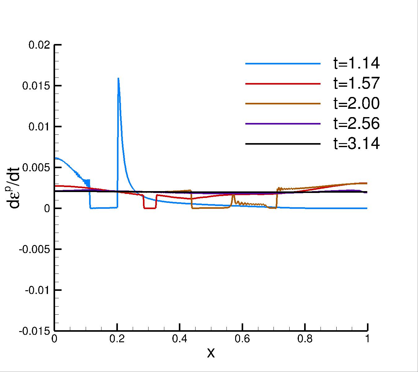
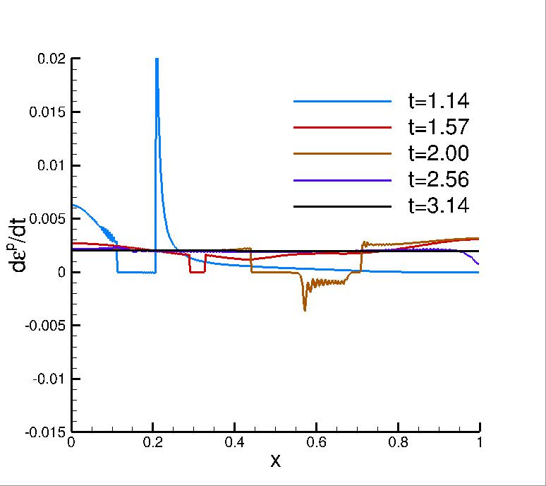
Figure 20: Plastic strain rate as a function of position at various normalized times. (a) $a_{2}=0.005$. (b) $a_{2}=-0.005$. (c) $a_{2}=-0.01$.

Time integration uses the explicit Newmark $\beta$ method with $\beta=0$, $\gamma=0.5$ and the stress update takes place via a linear incremental update

$$\sigma(t+\Delta t)=\sigma(t)+\dot{\sigma}(t)(\Delta t)$$ (62)

Assuming that plastic deformation makes no contribution to the internal energy, the local dissipation rate, Eq. (11), is given by

$$\dot{\xi}=|\sigma|\dot{\epsilon}^{p}=|\sigma|\dot{a}\left(\frac{|\sigma|}{\sigma_{0}}\right)^{m}$$ (63)

From the expression for the dissipation rate, $\dot{\xi}$, in Eq. (63) it is seen that the sign of $\dot{\xi}$ is the sign of $\dot{\epsilon}^{p}$ and hence of $\dot{a}$. For the calculations with $\dot{a}_{2}<0$, there is a time interval over which the dissipation rate is negative so that the Clausius-Duhem inequality is violated.

Plots of plastic strain rate $\dot{\epsilon}^{p}$ versus position $x$ at various times are shown for the three calculations in Fig. 20. In all three plots, the spatial distribution of $\dot{\epsilon}^{p}$ is qualitatively similar, although in Fig. 20a, where $\dot{a}_{2}>0$, the peak value of $\dot{\epsilon}^{p}$ i is smaller. In Fig. 20a, $\dot{\xi}>0$ for all time and all values of $x$. With increasing time, viscoplasticity damps out the propagating waves and a quasi-static uniform distribution of plastic strain is reached.

With $\dot{a}_{2}=-0.005$, Fig. 20b, the distribution of $\dot{\epsilon}^{p}$ shows there is an interval of $x$, the size of which is set by the propagating wave, for which $\dot{\xi}<0$ so that the Clausius-Duhem inequality is violated. Nevertheless, with increasing time viscoplastic dissipation eventually dominates and a stable quasi-static distribution of $\dot{\epsilon}^{p}$ develops as for the calculation with $\dot{a}_{2}=0.005$ in Fig. 20a. On the other hand, in Fig. 20c with $\dot{a}=-0.01$, the increased negative dissipation rate for the time interval $t_{0}\geq t\geq t_{0}+t_{c}$ leads to the overall response becoming unstable before $\dot{a}$ becomes positive again and viscoplastic damping can dominate.

Even in this simple examples whether or not a stable response will ultimately emerge depends on a wide variety of parameters other than $\dot{a}_{2}$, such as $t_{c}$ which sets the time interval over which a negative dissipation rate can occur, the specification of the applied loading which affects the interval over which a negative dissipation rate can occur, and the material strain and strain rate hardening which govern the viscoplastic damping. Nevertheless, this simple example illustrates that a stable overall response can be obtained using a conventional continuum constitutive relation that gives rise to a negative dissipation rate over a small interval for a short time.

The effect of negative dissipation rate on propagating waves was also investigated by Ostoja-Starzewski and Malyarenko (2014) through an analysis of one-dimensional acceleration waves with the wave amplitude governed by a Bernoulli equation evolving on a random field of dissipation rate. While the mean of that field was positive, the possibility of negative dissipation rate was allowed for and it was found that the probability of a wave amplitude blow-up event varied with the wavefront thickness, with a blow-up event being less probable for a thicker wavefront.

7.2 Discrete defect plasticity with a negative dissipation rate

The strong limitation on STZ transformation strains imposed by requiring a non-negative dissipation rate together with the results of atomistic modeling and experiment indicating larger transformation strains motivates the development of a kinetic relation for discrete defect plasticity that can have a negative dissipation rate (i.e. violate the Clausius-Duhem inequality) locally.

To illustrate a possible such relation for plane strain discrete STZ plasticity, an extension of Eq. (49) is

$$\dot{\gamma}^{*K}=\begin{cases}\frac{1}{B_{1}^{K}}\left(\gamma^{*K}_{\rm max}-\gamma^{*K}\right)\,&\mbox{for }\gamma^{*K}\leq\gamma^{*K}_{\rm c}\\ \frac{1}{B_{2}^{K}}\left(\gamma^{*K}_{\rm non}-\gamma^{*K}\right)\,&\mbox{for}\ t_{c}\leq t\leq t_{c}+t_{f}\\ 0\,&\mbox{for }t>t_{c}+t_{f}\ \mbox{or}\ \gamma^{*K}>\gamma^{*K}_{\rm non}\end{cases}$$ (64)

Here, $B^{K}_{\alpha}>0$ ($\alpha=1,2$), $\gamma^{*K}_{\rm non}$ is a specified transformation strain greater than the value of $\gamma^{*K}_{\rm max}$ given by Eq. (50), $\gamma^{*K}_{\rm c}\leq\gamma^{*K}_{\rm max}$, $t_{c}$ is the first time at which $\gamma^{*K}=\gamma^{*K}_{\rm c}$, $t_{f}$ is a specified time interval during which a negative dissipation rate is allowed.

The dissipation rate is then given by

$$\dot{\cal{D}}^{K}(t)=\begin{cases}C^{K}_{1}\left(\gamma^{*K}_{\rm max}-\gamma^{*K}\right)^{2}\ &\mbox{for }{\gamma}^{*K}\leq{\gamma}^{*K}_{\rm c}\\ C^{K}_{2}\left(\gamma^{*K}_{\rm max}-\gamma^{*K})(\gamma^{*K}_{\rm non}-\gamma^{*K}\right),&\mbox{for}\ t_{c}\leq t\leq t_{c}+t_{f}\\ 0\,&\mbox{for }t>t_{c}+t_{f}\ \mbox{or}\ \gamma^{*K}>\gamma^{*K}_{\rm non}\end{cases}$$ (65)

where

$$C^{K}_{\alpha}=\frac{EA^{K}_{\rm incl}}{2(1-\nu^{2})B^{K}_{\alpha}}\qquad\alpha=1,2$$ (66)

Hence, when $\gamma^{*K}_{\rm max}<\gamma^{*K}<\gamma^{*K}_{\rm non}$ for some time period in the interval $t_{c}\leq t\leq t_{c}+t_{f}$, $\dot{\cal{D}}^{K}<0$ during that time period.

A distribution of values of $\gamma^{*K}_{\rm c}$ can be specified so that there is some non-zero probability that $\gamma^{*K}>\gamma^{*K}_{\rm c}$ in some STZs. Similarly for discrete dislocation plasticity, the expression for dislocation velocity, such as in Eq. (34) or Eq. (35), can be taken to apply for a range of stress magnitudes and/or a range of values of dislocation velocity via expressions analogous to Eq. (65) so that some values of $\dot{\cal{D}}^{K}$ in Eq. (36) could be permitted to take on negative values with a specified probability. This could require the Clausius-Duhem inequality to be satisfied for the body as a whole, Eq. (10), but allow the local condition, Eq. (11) to be violated for some sufficiently small time interval.

Li et al. (2019); Montefusco et al. (2021) have used data from a lower level calculation together with a statistical mechanics fluctuation dissipation relation as a basis for computing dissipative evolution equations/dissipation potentials. It may be possible to extend such an approach to: (i) use lower level calculations for the development of discrete defect plasticity kinetic relations, and/or (ii) use discrete defect plasticity calculations for the development of continuum plasticity constitutive relations.

8 Concluding remarks

The partitioning between defect elastic energy storage and defect dissipation can play a major role in a wide variety of phenomena of technological significance, including friction, fracture, fatigue, thermal softening and the Bauschinger effect. The predicted partitioning of energy and its size dependence are dependent on a wide variety of factors including, for example, stress state, loading rate, loading mode, e.g. monotonic loading versus cyclic loading, and size, as well, of course, as on the kinetic relations used to model defect evolution. The few discrete defect calculations of the evolution of dissipation and its possible size effect that have been carried out show that discrete defect plasticity can provide insight into mechanical behaviors where the evolution of dissipation plays a significant role. No such calculations have been carried out that allow for the possibility that the Coleman-Noll postulate (Coleman and Noll, 1964), i.e. that the Clausius-Duhem inequality must be satisfied for all points of a body for all time, does not hold. Discrete defect calculations of possible effects of local violations of the Clausius-Duhem inequality on predictions of friction, fracture, fatigue, thermal softening and the Bauschinger effect merit exploration.

The partitioning between stored elastic energy and dissipation and its size dependence can vary with the mode of defect evolution. In the circumstances considered, when defect evolution occurred by defects that move relatively long distances, the energy partitioning involved significant dissipation and the plastic response was size dependent; when defect evolution occurred by the nucleation of more or less stationary defects from fixed nucleation site the energy partitioning involved little dissipation and the plastic response had nearly no size independence; and when defect evolution occurred by the nucleation of stationary defects from sites that increased in a percolation-like manner, the energy partitioning involved significant dissipation and the plastic response had little size independence.

It is worth noting that statistical effects in addition to fluctuations can play an important role in discrete defect plasticity. For example, in both discrete dislocation plasticity and discrete STZ plasticity, the initial conditions and defect nucleation/evolution parameters are specified by statistical distributions, for example, a random spatial distribution of initial nucleation sites and a random distribution of nucleation strengths. Furthermore, the interaction of discrete defects can be chaotic, as found for discrete dislocation plasticity by Deshpande et al. (2001). The predicted overall response can be sensitive to details of the statistical variations and even for macro size material regions statistical variations can induce local changes in defect structure that have a large effect. For example, variations in the location of defects in the vicinity of a crack tip can affect the predicted crack growth resistance. Quantitative discrete defect plasticity characterizations of the effect of statistical variations on material response and, in particular, of the effect on the evolution of energy partitioning, are needed.

For discrete STZ plasticity, requiring a non-negative dissipation rate for all Eshelby transformations for all time imposes a strong limit on the allowed transformation strain magnitude. Accounting for an associated entropy increase could allow for larger transformation strains by the term $\dot{s}\Theta$ being sufficiently positive so that the Clausius-Duhem inequality is satisfied even if the mechanical dissipation rate is negative and/or there could be a substantial entropy induced reduction in stiffness in the STZ. However, an STZ transformation involves a relatively small number of atoms and the transformation takes place over a relatively short period of time. Hence, it is also possible that requiring satisfaction of the Clausius-Duhem inequality for all Eshelby transformations for all time is overly restrictive.

Because, at least in some contexts, the Clausius-Duhem inequality is a stability condition, e.g. Coleman and Mizel (1967); Dafermos (1979), the question arises as to whether or not the Clausius-Duhem inequality is more broadly a stability condition and, if so, whether stability (in some appropriate sense) can be maintained in discrete defect calculations if the Clausius-Duhem inequality is violated locally. In the simple one-dimensional analysis in Section 7.1 overall stability was maintained when the dissipation rate was negative (but not too negative) locally for a short time. Such calculations for discrete defect plasticity remain to be carried out. A suitable continuum mechanics expression of the second law of thermodynamics for discrete defect plasticity that allows the Clausius-Duhem inequality to be violated locally (while maintaining overall stability) remains to be developed. One possibility is to require $\int\sum\dot{\cal{D}}^{K}dt\geq 0$ or even each $\int\dot{\cal{D}}^{K}dt\geq 0$ for some specified time interval using relations like Eq. (36) or Eq. (65).

In a wide variety of contexts, continuum mechanics is being used to model the evolution of inelastic deformation of “small” and/or “soft” materials and systems. In such systems, fluctuations can play a role and frameworks to allow fluctuation effects to be accounted for in formulating continuum constitutive relations are being developed, Ostoja-Starzewski (2016); Li et al. (2019); Montefusco et al. (2021). Indeed, it is now well-appreciated that assumptions underlying continuum mechanics formulations for modeling “large” material regions and systems, such as the assumption of a size independent constitutive response, need to be abandoned to model “small” scale material/system response. For discrete defect plasticity (and perhaps more broadly for a variety of “small/soft” materials and systems) it may be necessary to develop continuum mechanics constitutive formulations that abandon the requirement that the Clausius-Duhem inequality is satisfied at all points of a body for all time.

References

- Albert et al. (2016) Albert, T., Tanguy, A., Boioli, F., Rodney, D., 2016. Mapping between atomistic simulations and Eshelby inclusions in the shear deformation of an amorphous silicon model. Phys. Rev. E 93, 053002.
- Argon (1979) Argon, A.S., 1979. Plastic deformation in metallic glasses. Acta Metall. 27, 47-58.
- Argon and Shi (1983) Argon, A.S., Shi, L.T., 1983. Development of visco-plastic deformation in metallic glasses. Acta Metall. 31, 499-507.
- Ayton et al. (2001) Ayton, G., Evans, D.J., Searles, D.J., 2001. A local fluctuation theorem. J. Chem. Phys. 115, 2033-2037.
- Benzerga et al. (2003) Benzerga, A.A., Bréchet, Y., Needleman, A., Van der Giessen, E., 2003. Incorporating three-dimensional mechanisms into two-dimensional dislocation dynamics. Modell. Simul. Mater. Sci. Engin. 12, 159-196.
- Benzerga et al. (2005) Benzerga,, A.A., Bréchet, Y., Needleman , A., Van der Giessen, E., 2004. The stored energy of cold work: predictions from discrete dislocation plasticity. Acta Mat. 53, 4765- 4779.
- Bouchbinder and Langer (2009) Bouchbinder, E., Langer, J.S., 2009. Nonequilibrium thermodynamics of amorphous materials II: Effective-temperature theory. Phys. Rev. E 80, 031132.
- Bulatov and Argon (1994) Bulatov, V.V., Argon, A.S., 1994. A stochastic model for continuum elasto-plastic behavior. I. numerical approach and strain localization. Modell. Simul. Mater. Sci. Engin. 2, 167-184.
- Cleveringa et al. (2000) Cleveringa, H.H.M., Van der Giessen, E., Needleman. A., 2000. A discrete dislocation analysis of mode I crack growth. J. Mech. Phys. Solids 48, 1133-1157.
- Coleman and Mizel (1967) Coleman, B.D., Mizel, V.J., 1967. Existence of entropy as a consequence of asymptotic stability. Arch. Rat. Mech. Analysis, 25, 243-270.
- Coleman and Noll (1964) Coleman, B.D., Noll, W., 1964. The thermodynamics of elastic materials with heat conduction and viscosity. Arch. Ration. Mech. Anal. 13, 167–178.
- Dafermos (1979) Dafermos, C.M., 1979. The second law of thermodynamics and stability. Arch. Rat. Mech. Analysis 70, 167-179.
- Dasgupta et al. (2013) Dasgupta, R., Hentschel, H.G.E., Procaccia, I., 2013. Yield strain in shear banding amorphous solids. Phys. Rev. E 87, 022810.
- Deshpande et al. (2001) Deshpande, V.S., Needleman. A., Van der Giessen, E., 2001. Dislocation dynamics is chaotic. Scripta Mat., 45, 1047-1053.
- Deshpande et al. (2003a) Deshpande, V.S., Needleman. A., Van der Giessen, E., 2003. Discrete dislocation plasticity modeling of short cracks in single crystals. Acta Mat. 51, 1-15.
- Deshpande et al. (2003b) Deshpande, V.S., Needleman. A., Van der Giessen, E., 2003. Finite strain discrete dislocation plasticity. J. Mech. Phys. Solids 51, 2057-2083.
- Deshpande et al. (2004) Deshpande, V.S., Needleman. A., Van der Giessen, E., 2004. Discrete dislocation plasticity analysis of static friction. Acta Mat. 52, 3135-3149.
- Deshpande et al. (2005) Deshpande, V.S., Needleman. A., Van der Giessen, E., 2005. Size dependence of energy storage and dissipation in a discrete dislocation plasticity analysis of static friction. Mat. Sci. Engin. A, 400-401, 393-396.
- Eshelby (1957) Eshelby, J.D., 1957. The determination of the elastic field of an ellipsoidal inclusion, and related problems. Proc. R. Soc. Lond. A 241, 376–396.
- Eshelby (1959) Eshelby, J.D., 1959. The elastic field outside an ellipsoidal inclusion. Proc. R. Soc. Lond. A 252, 561–569.
- Evans et al. (1993) Evans, D.J., Cohen, E.G.D., Morriss, G.P., 1993. Probability of second law violations in shearing steady states. Phys. Rev. Letts., 71, 2401-2404, 1993.
- Evans and Searles (2002) Evans, D.J., Searle, D.J., 2002. The fluctuation theorem. Adv. Phys. 51, 1529-1585.
- Falk and Langer (2011) Falk, M.L., Langer, J.S., 2011. Deformation and failure of amorphous, solidlike materials. Ann. Rev. Condens. Matter Phys. 2, 353-373.
- Hodowany et al. (2000) Hodowany, J., Ravichandran, G., Rosakis, A.J., Rosakis, P., 2000. Partition of plastic work into heat and stored energy in metals. Exp. Mech. 40, 113–23.
- Hufnagel et al. (2016) Hufnagel, T.C., Schuh, C.A., Falk, M.L., 2016. Deformation of metallic glasses: Recent developments in theory, simulations, and experiments. Acta Mat. 109, 375-393.
- Hussein et al. (2015) Hussein, A.M., Rao, S.I., Michael Uchic, D., Dimiduk, D.M., El-Awady, J.A., 2015. Microstructurally based cross-slip mechanisms and their effects on dislocation microstructure evolution in fcc crystals. Acta Mat. 85, 180–190.
- Irani et al. (2015) Irani, N., Remmers, J.J.C., Deshpande, V.K., 2015. Finite strain discrete dislocation plasticity in a total Lagrangian setting. J. Mech. Phys. Solids 83, 160-178.
- Jarzynski (2010) Jarzynski, C., 2010. Equalities and inequalities: irreversibility and the second law of thermodynamics at the nanoscale. Séminaire Poincaré XV Le Temps, 77–102.
- Kondori et al. (2018) Kondori, B., Benzerga, A.A., Needleman A., 2018. Discrete shear-transformation-zone plasticity modeling of notched bars. J. Mech. Phys. Solids 111, 18-42 (Erratum, 127, 151-153, 2019).
- Li et al. (2019) Li, X., Dirr,N., Embacher, P., Zimmer, J., Reina, C., 2019. Harnessing fluctuations to discover dissipative evolution equations. J. Mech. Phys. Solids 131, 240-251.
- Lubarda et al. (1993) Lubarda, V.A., Blume, J.A., Needleman, A., 1993. An analysis of equilibrium dislocation distributions. Acta Metall. Mater. 41, 625-642.
- Mass and Löffler (2015) Maass, R., Löffler, J.F., 2015. Shear-band dynamics in metallic glasses. Adv. Funct. Mater. 25, 2353-2368.
- Malka-Markovitz et al. (2021) Malka-Markovitz, A., Devincre, B., Mordehai, D., 2021. A molecular dynamics-informed probabilistic cross-slip model in discrete dislocation dynamics. Scripta Mat. 190, 7–11.
- Montefusco et al. (2021) Montefusco, A., Peletier, M.A., Öttinger, H.C., 2021 A framework of nonequilibrium statistical mechanics. II. Coarse-graining. J. Non-Equilib. Thermodyn. 46, 15–33.
- Ostoja-Starzewski (2016) Ostoja-Starzewski, M., 2016. Second law violations, continuum mechanics, and permeability. Continuum Mech. Thermodyn. 28, 489–-501 (Erratum 29, 359, 2017).
- Ostoja-Starzewski and Laudani (2020) Ostoja-Starzewski, M., Laudani, R., 2020. Violations of the Clausius–Duhem inequality in Couette flows of granular media. Proc. R. Soc. A476, 20200207.
- Ostoja-Starzewski and Malyarenko (2014) Ostoja-Starzewski, M., Malyarenko, A., 2014. Continuum mechanics beyond the second law of thermodynamics. Proc. R. Soc. A470, 20140531.
- Qin and Bassani (1992) Qin, Q., Bassani, J.L., 1992. Non-Schmid yield behavior in single crystals. J. Mech. Phys. Solids 40, 813-833.
- Qu et al. (2015) Qu, R.T., Liu, Z. Q., Wang, R. F., and Zhang, Z. F., 2015. Yield strength and yield strain of metallic glasses and their correlations with glass transition temperature. J. Alloys Compd. 637 . 44–54.
- Shu et al. (2001) Shu, J.Y., Fleck, N.A., Van der Giessen, E., Needleman, A., 2001. Boundary layers in constrained plastic flow: comparison of nonlocal and discrete dislocation plasticity. J. Mech. Phys. Solids 49, 1361-1395.
- Spaepen (1977) Spaepen, F., 1977. A microscopic mechanism for steady state inhomogeneous flow in metallic glasses. Acta Metal. 25, 407–415.
- Suresh (1991) Suresh, S. 1991. Fatigue of materials. Cambridge University Press, Cambridge UK.
- Van der Giessen and Needleman (1995) Van der Giessen, E., Needleman, A., 1995. Discrete dislocation plasticity: a simple planar model. Model. Simul. Mater. Sci. Engng. 3, 689-735.
- Vasoya et al. (2019) Vasoy, M., Kondori, B., Benzerga, A.A., Needleman, A., 2019. Limits on transformation strains for non-negative dissipation. J. Appl. Mech. 86, 051005.
- Vasoya et al. (2020) Vasoya, M., Kondori, B., Benzerga, A.A., Needleman, A., 2020. Energy dissipation rate and kinetic relations for Eshelby transformations. J. Mech. Phys. Solids 136, 103699.
- Vasoya et al. (2021) Vasoya, M., Benzerga, A.A., Needleman, A., 2021. Shear Transformation Zone (STZ) plasticity analysis of constrained shear. Mech. Mater. 160, 103935.
- Vitek et al. (2004) Vitek, V., Mrovec, M., Bassani, J.L., 2004. Influence of non-glide stresses on plastic flow: from atomistic to continuum modeling. Mater. Sci. Engin. A365, 31-37.
- Vitek and Paidar (2008) Vitek, V., Paidar, V., 2008. Non-planar dislocation cores: a ubiquitous phenomenon affecting mechanical properties of crystalline materials. in: Dislocations in Solids,ed. J.P. Hirth, Ch. 87, Elsevier, Amsterdam.
- Wang et al. (2010) Wang, G.M., Sevick, E.M., Mittag, E., Searles, D.J., Evans, D.J., 2010. Experimental demonstration of violations of the second law of thermodynamics for small systems and short time scales. Phys. Rev. Letts. 89, 050601.
- Wang and Beyerein (2011) Wang, Z.Q., Beyerlein, I.J., 2011. An atomistically-informed dislocation dynamics model for the plastic anisotropy and tension–compression asymmetry of BCC metals. Int. J. Plast. 27, 1471-1484.