Efficient evaluation of double-barrier options and joint cpdf of a Lévy process and its two extrema

Abstract.

In the paper, we develop a very fast and accurate method for pricing double barrier options with continuous monitoring in wide classes of Lévy models; the calculations are in the dual space, and the Wiener-Hopf factorization is used. For wide regions in the parameter space, the precision of the order of $10^{-15}$ is achievable in seconds, and of the order of $10^{-9}-10^{-8}$ - in fractions of a second. The Wiener-Hopf factors and repeated integrals in the pricing formulas are calculated using sinh-deformations of the lines of integration, the corresponding changes of variables and the simplified trapezoid rule. If the Bromwich integral is calculated using the Gaver-Wynn Rho acceleration instead of the sinh-acceleration, the CPU time is typically smaller but the precision is of the order of $10^{-9}-10^{-6}$, at best. Explicit pricing algorithms and numerical examples are for no-touch options, digitals (equivalently, for the joint distribution function of a Lévy process and its supremum and infimum processes), and call options. Several graphs are produced to explain fundamental difficulties for accurate pricing of barrier options using time discretization and interpolation-based calculations in the state space.

Key words: Lévy process, extrema of a Lévy process, double barrier options, Fourier transform, Gaver-Wynn Rho algorithm, sinh-acceleration

MSC2020 codes: 60-08,42A38,42B10,44A10,65R10,65G51,91G20,91G60

1. Introduction

Let $X$ be a one-dimensional Lévy process on the filtered probability space $({\Omega},{\mathcal{F}},\{{\mathcal{F}}_{t}\}_{t\geq 0},{\mathbb{Q}})$ satisfying the usual conditions. We denote the expectation operator under ${\mathbb{Q}}$ by ${\mathbb{E}}$. In a number of publications, various methods were applied to calculation of expectations $V(f;T;x_{1},x_{2})$ of functions of spot value $x_{1}$ of $X$ and its running maximum or minimum $x_{2}$ and related optimal stopping problems, standard examples being barrier and American options, and lookback options with barrier and/or American features. See, e.g., [35, 13, 14, 15, 44, 5, 6, 40, 39, 7, 9, 10, 42, 41, 8, 20, 36, 34, 37, 48, 33, 47, 21, 25, 27] and the bibliographies therein. Options with discrete and continuous monitoring were considered.

In the paper, we develop very fast and accurate method for pricing double barrier options with continuous monitoring in Lévy models, without rebate: if the underlying factor $X$ breaches one of the two barriers $h_{-}<h_{+}$ before or on the maturity date $T$, the option expires worthless. In neither of the barriers are breached, the payoff is $G(X_{T})$. The method of the paper can be modified to the case of double barrier options with rebate and to the case of options with discrete monitoring. Pricing barrier options without rebate trivially reduces to the calculation of expectations in a model with 0 interest rate $r$, hence, in the main body of the paper, we assume that $r=0$, and allow ${\mathbb{Q}}$ to be not an equivalent martingale measure. Explicit algorithms are formulated and numerical examples produced for no-touch options, double barrier options with digital payoff (equivalently, joint pdf of $X_{T}$, the infimum process ${\underline{X}}_{t}=\inf_{0\leq s\leq t}X_{s}$ and supremum process ${\bar{X}}_{t}=\sup_{0\leq s\leq t}X_{s}$), and double barrier call options.

At the first step, we impose no condition on the Lévy process, and assume that the payoff function $G$ is measurable and bounded. Denote by $V(G;h_{-},h_{+};T,x)$ the price of the option. We represent the Laplace transform ${\tilde{V}}(G;h_{-},h_{+};q,x)$ of the price in the form of a sum of the present value of the perpetual stream $G(X_{t})$, the discount rate being $q$, and the sum of two series of prices of perpetual first touch options. As in [10], we represent the prices of the perpetual options using the technique of the expected present value operators (EPV operators) developed in a series of publications [13, 14, 15, 17, 9]. The EPV technique is the operator form of the Wiener-Hopf factorization. In op.cit. as well in a number of other publications where the EPV technique was used, the numerical realization is in the state space. If the calculations are in the state space, the precision of the order of $10^{-6}$ is very difficult to achieve unless high precision arithmetic is used. In [20, 45], the calculations are in the dual space. The fractional-parabolic deformations of the contours of integration at each step of the iteration procedure allow one to calculate the integrals in the formulas for the value functions using the simplified trapezoid rule with large but not exceedingly large number of terms. In the result, it is possible to achieve a precision better that $10^{-6}$. However, in some cases, the accumulated errors of calculation of dozens of thousand of terms are too large to achieve a higher precision.

In the present paper, we apply a more efficient family of sinh-deformations used in [22] to price European options in Lévy and affine models and in [24, 25] to price single barrier options and lookback options. After appropriate conformal deformations of the contours of integration and the corresponding changes of variables, we evaluate the resulting repeated integrals applying the simplified trapezoid rule to each integral. The analyticity of the integrands around the line of integration imply that the error of the infinite trapezoid rule decays as the exponential of $-1/\zeta$, where $\zeta$ is the step of the trapezoid rule (see, e.g., Theorem 3.2.1 in [49]); the sinh-change of variable lead to integrands which decay faster than the exponential function, hence, the truncation error decays faster than the discretization error. For the Laplace inversion, we use two methods: the Gaver-Wynn Rho acceleration algorithm (GWR algorithm), and the sinh-acceleration, as in [25]; earlier, we applied a less efficient fractional-parabolic deformations [20]. The method of the paper can be regarded as a further step in a general program of study of the efficiency of combinations of one-dimensional inverse transforms for high-dimensional inversions systematically pursued by Abate-Whitt, Abate-Valko [2, 3, 1, 51, 4] and other authors. Additional methods can be found in [49]. The sinh-acceleration is simpler to apply than the saddle-point method (see., e.g., [32]), and the calculation of individual terms in numerical realizations is much simpler and less time consuming. The former method is more flexible than the latter, in applications to repeated integrals especially. The rates of convergence of the sinh-acceleration method and saddle point method are approximately the same. Talbot’s deformation [50] is not applicable together with the sinh-deformations of the other contours of integration, hence, the CPU time is significantly larger and good precision is impossible to achieve in many cases where the method of the paper is very efficient.

The rest of the paper is organized as follows. In Section 2, we recall the basic facts of the Wiener-Hopf factorization technique, the definitions of the classes of Lévy processes amenable to efficient calculations, and efficient formulas for the Wiener-Hopf factors. In Section 3, we reproduce the iteration procedure for evaluation of the Laplace transform of the price in terms of the EPV-operators (factors in the operator form of the Wiener-Hopf factorization) derived in [10], and then design efficient procedure in the dual space, which significantly improves the procedure used in [45]. Explicit algorithms for the double no-touch, digital and call options are in Section 4. Numerical examples are discussed in Section 5; the figures and tables are relegated to Section A. We plot several graphs to demonstrate fundamental difficulties for accurate pricing of barrier options using time discretization and interpolation-based calculations in the state space. In Section 6, we summarize the results and outline possible applications of the method of the paper.

2. Auxilliary results

2.1. Wiener-Hopf factorization

2.1.1. General formulas for the Wiener-Hopf factors

For $q>0$, let $T_{q}\sim\operatorname{Exp}q$ be an exponentially distributed random variable with mean $q^{-1}$, independent of $X$. In probability, the Wiener-Hopf factors are defined as

(2.1) $$\phi^{+}_{q}(\xi)={\mathbb{E}}[e^{i\xi{\bar{X}}_{T_{q}}}],\quad\phi^{-}_{q}(\xi)={\mathbb{E}}[e^{i\xi{\underline{X}}_{T_{q}}}].$$

Functions $\phi^{\pm}_{q}(\xi)$ appear in the Wiener-Hopf factorization formula

(2.2) $$\frac{q}{q+\psi(\xi)}=\phi^{+}_{q}(\xi)\phi^{-}_{q}(\xi),\quad\xi\in{\mathbb{R}},$$

which is a special case of the Wiener-Hopf factorization of functions of more general classes. Define the expected present value operators (EPV-operators) under $X$, ${\bar{X}}$ and ${\underline{X}}$ (all three start at 0) by ${\mathcal{E}}_{q}u(x)={\mathbb{E}}\left[u(x+X_{T_{q}})\right]$, ${\mathcal{E}}^{+}_{q}u(x)={\mathbb{E}}\left[u(x+{\bar{X}}_{T_{q}})\right]$ and ${\mathcal{E}}^{-}_{q}u(x)={\mathbb{E}}\left[u(x+{\underline{X}}_{T_{q}})\right]$. Clearly, the EPV operators are bounded operators in $L_{\infty}({\mathbb{R}})$. In the case of Lévy processes with exponentially decaying Lévy densities, the EPV operators are bounded operators in spaces with exponential weights. For details, see [14, 9, 10]. The operator version of (2.2)

(2.3) $${\mathcal{E}}_{q}={\mathcal{E}}^{+}_{q}{\mathcal{E}}^{-}_{q}={\mathcal{E}}^{-}_{q}{\mathcal{E}}^{+}_{q}$$

is a special case of the operator form of the Wiener-Hopf factorization in the theory of boundary problems for differential and pseudo-differential operators (pdo). Indeed, ${\mathcal{E}}^{\pm}_{q}e^{ix\xi}=\phi^{\pm}_{q}(\xi)e^{ix\xi}$. This means that ${\mathcal{E}}^{\pm}_{q}$ are pdo with symbols $\phi^{\pm}_{q}$, and ${\mathcal{E}}^{\pm}_{q}u(x)={\mathcal{F}}^{-1}_{\xi\to x}\phi^{\pm}_{q}(\xi){\mathcal{F}}_{x\to\xi}u(x)$ for sufficiently regular functions $u$. See, e.g., [31]. The Wiener-Hopf factor $\phi^{+}_{q}(\xi)$ (resp., $\phi^{-}_{q}(\xi)$) admits analytic continuation to the half-plane $\{\operatorname{\rm Im}\xi>0\}$ (resp., $\{\operatorname{\rm Im}\xi<0\}$).

The characteristic exponents of all popular classes of Lévy processes bar stable Lévy processes admit analytic continuation to a strip around the real axis. See [14, 13, 15], where the general class of Regular Lévy processes of exponential type (RLPE) is introduced. Let $X$ be a Lévy process with the characteristic exponent admitting analytic continuation to a strip $\{\operatorname{\rm Im}\xi\in(\mu_{-},\mu_{+})\}$ around the real axis, and let $q>0$. Then (see., e.g., [14, 13, 45]) the following statements hold

I. There exist $\sigma_{-}(q)<0<\sigma_{+}(q)$ such that

(2.4) $$q+\psi(\eta)\not\in(-\infty,0],\quad\operatorname{\rm Im}\eta\in(\sigma_{-}(q),\sigma_{+}(q)).$$

II. The Wiener-Hopf factor $\phi^{+}_{q}(\xi)$ admits analytic continuation to the half-plane $\{\operatorname{\rm Im}\xi>\sigma_{-}(q)\}$, and can be calculated as follows: for any $\omega_{-}\in(\sigma_{-}(q),\operatorname{\rm Im}\xi)$,

(2.5) $$\phi^{+}_{q}(\xi) = \exp\left[\frac{1}{2\pi i}\int_{\operatorname{\rm Im}\eta=\omega_{-}}\frac{\xi\ln(1+\psi(\eta)/q)}{\eta(\xi-\eta)}d\eta\right].$$

III. The Wiener-Hopf factor $\phi^{-}_{q}(\xi)$ admits analytic continuation to the half-plane $\{\operatorname{\rm Im}\xi<\sigma_{+}(q)\}$, and can be calculated as follows: for any $\omega_{+}\in(\operatorname{\rm Im}\xi,\sigma_{+}(q))$,

(2.6) $$\phi^{-}_{q}(\xi) = \exp\left[-\frac{1}{2\pi i}\int_{\operatorname{\rm Im}\eta=\omega_{+}}\frac{\xi\ln(1+\psi(\eta)/q)}{\eta(\xi-\eta)}d\eta\right].$$

We can (and will) use (2.2) and (2.5) to calculate ${\phi^{-}_{q}}(\xi)$ on $\{\operatorname{\rm Im}\xi\in(0,\sigma^{+}_{q})\}$, and (2.2) and (2.6) to calculate ${\phi^{+}_{q}}(\xi)$ on $\{\operatorname{\rm Im}\xi\in(\sigma^{-}_{q},0)\}$.

2.2. General classes of Lévy processes amenable to efficient calculations

Essentially all popular classes of Lévy processes processes enjoy additional properties formalized in [22, 28].

For $\nu=0+$ (resp., $\nu=1+$), set $|\xi|^{\nu}=\ln|\xi|$ (resp., $|\xi|^{\nu}=|\xi|\ln|\xi|$), and introduce the following complete ordering in the set $\{0+,1+\}\cup(0,2]$: the usual ordering in $(0,2]$; $\forall\ \nu>0,0+<\nu$; $\forall\ \nu>1,1<1+<\nu$. For $\gamma\in(0,\pi]$, $\pm\gamma_{\pm}\in(0,\pi 2]$ and $\mu_{-}<\mu_{+}$, define ${\mathcal{C}}_{\gamma_{-},\gamma_{+}}=\{e^{i\varphi}\rho\ |\ \rho>0,\varphi\in(\gamma_{-},\gamma_{+})\cup(\pi-\gamma_{+},\pi-\gamma_{-})\}$, ${\mathcal{C}}_{\gamma}=\{e^{i\varphi}\rho\ |\ \rho>0,\varphi\in(-\gamma,\gamma)\}$, $S_{(\mu_{-},\mu_{+})}=\{\xi\ |\ \operatorname{\rm Im}\xi\in(\mu_{-},\mu_{+})\}$.

Definition 2.1.

([28, Defin 2.1]) We say that $X$ is a SINH-regular Lévy process (on ${\mathbb{R}}$) of order $\nu$ and type $((\mu_{-},\mu_{+});{\mathcal{C}};{\mathcal{C}}_{+})$ iff the following conditions are satisfied:

1. $\nu\in\{0+,1+\}\cup(0,2]$ and $\mu_{-}<0\leq\mu_{+}$ or $\mu_{-}\leq 0<\mu_{+}$;

2. ${\mathcal{C}}={\mathcal{C}}_{\gamma_{-},\gamma_{+}},{\mathcal{C}}_{+}={\mathcal{C}}_{\gamma^{\prime}_{-},\gamma^{\prime}_{+}}$, where $\gamma_{-}<0<\gamma_{+}$, $\gamma_{-}\leq\gamma^{\prime}_{-}\leq 0\leq\gamma^{\prime}_{+}\leq\gamma_{+}$, and $|\gamma^{\prime}_{-}|+\gamma^{\prime}_{+}>0$;

3. the characteristic exponent $\psi$ of $X$ can be represented in the form

   (2.7) $$\psi(\xi)=-i\mu\xi+\psi^{0}(\xi),$$

   where $\mu\in{\mathbb{R}}$, and $\psi^{0}$ admits analytic continuation to $i(\mu_{-},\mu_{+})+({\mathcal{C}}\cup\{0\})$;

4. for any $\varphi\in(\gamma_{-},\gamma_{+})$, there exists $c_{\infty}(\varphi)\in{\mathbb{C}}\setminus(-\infty,0]$ s.t.

   (2.8) $$\psi^{0}(\rho e^{i\varphi})\sim c_{\infty}(\varphi)\rho^{\nu},\quad\rho\to+\infty;$$

5. the function $(\gamma_{-},\gamma_{+})\ni\varphi\mapsto c_{\infty}(\varphi)\in{\mathbb{C}}$ is continuous;

6. for any $\varphi\in(\gamma^{\prime}_{-},\gamma^{\prime}_{+})$, $\operatorname{\rm Re}c_{\infty}(\varphi)>0$.

To simplify the constructions in the paper, we assume that $\mu_{-}<0<\mu_{+}$ and $\gamma^{\prime}_{-}<0<\gamma^{\prime}_{+}$.

Example 2.2.

In [11, 12], we constructed a family of pure jump processes generalizing the class of [38], with the Lévy measure

(2.9) $$F(dx)=c_{+}e^{\lambda_{-}x}x^{-\nu_{+}-1}{\bf 1}_{(0,+\infty)}(x)dx+c_{-}e^{\lambda_{+}x}|x|^{-\nu_{-}-1}{\bf 1}_{(-\infty,0)}(x)dx,$$

where $c_{\pm}>0,\nu_{\pm}\in[0,2),\lambda_{-}<0<\lambda_{+}$. If $\nu_{\pm}\in(0,2),\nu_{\pm}\neq 1$,

(2.10) $$\psi^{0}(\xi)=c_{+}\Gamma(-\nu_{+})((-\lambda_{-})^{\nu_{+}}-(-\lambda_{-}-i\xi)^{\nu_{+}})+c_{-}\Gamma(-\nu_{-})(\lambda_{+}^{\nu_{-}}-(\lambda_{+}+i\xi)^{\nu_{-}}).$$

A specialization $\nu_{\pm}=\nu\neq 1$, $c=c_{\pm}>0$, of KoBoL used in a series of numerical examples in [11] was named CGMY model in [30] (and the labels were changed: letters $C,G,M,Y$ replace the parameters $c,\nu,\lambda_{-},\lambda_{+}$ of KoBoL):

(2.11) $$\psi^{0}(\xi)=c\Gamma(-\nu)[(-\lambda_{-})^{\nu}-(-\lambda_{-}-i\xi)^{\nu}+\lambda_{+}^{\nu}-(\lambda_{+}+i\xi)^{\nu}].$$

Evidently, $\psi^{0}$ given by (2.11) is analytic in ${\mathbb{C}}\setminus i{\mathbb{R}}$, and $\forall\ \varphi\in(-\pi/2,\pi/2)$, (2.8) holds with

(2.12) $$c_{\infty}(\varphi)=-2c\Gamma(-\nu)\cos(\nu\pi/2)e^{i\nu\varphi}.$$

In [28], we defined a class of Stieltjes-Lévy processes (SL-processes). Essentially, $X$ is called a (signed) SL-process if $\psi$ is of the form

(2.13) $$\psi(\xi)=(a^{+}_{2}\xi^{2}-ia^{+}_{1}\xi)ST({\mathcal{G}}^{0}_{+})(-i\xi)+(a^{-}_{2}\xi^{2}+ia^{-}_{1}\xi)ST({\mathcal{G}}^{0}_{-})(i\xi)+(\sigma^{2}/2)\xi^{2}-i\mu\xi,$$

where $ST({\mathcal{G}})$ is the Stieltjes transform of the (signed) Stieltjes measure ${\mathcal{G}}$, $a^{\pm}_{j}\geq 0$, and $\sigma^{2}\geq 0$, $\mu\in{\mathbb{R}}$. A (signed) SL-process is called regular if it is SINH-regular. We proved in [28] that the characteristic exponent $\psi$ of a (signed) SL-process admits analytic continuation to the complex plane with two cuts along the imaginary axis. If $X$ is SL-process, then, for any $q>0$, equation $q+\psi(\xi)=0$ has no solution on ${\mathbb{C}}\setminus i{\mathbb{R}}$. We proved that all popular classes of Lévy processes bar the Merton model and Meixner processes are regular SL-processes, with $\gamma_{\pm}=\pm\pi/2$; the Merton model and Meixner processes are regular signed SL-processes, and $\gamma_{\pm}=\pm\pi/4$. In [28], the reader can find a list of SINH-processes and SL-processes, with calculations of the order and type.

2.3. Evaluation of the Wiener-Hopf factors and sinh-acceleration

The integrands on the RHSs of (2.5) and (2.6) decay very slowly at infinity, hence, it is impossible to achieve a good precision without additional tricks. If $X$ is SINH-regular, the rate of decay of the integrands can be significantly increased using appropriate conformal deformations of the line of integration and the corresponding changes of variables. Assuming that in Definition 2.1, $\gamma_{\pm}$ are not extremely small is absolute value (and, in the case of regular SL-processes, $\gamma_{\pm}=\pm\pi/2$ are not small), the most efficient change of variables is the sinh-acceleration

(2.14) $$\eta=\chi_{\omega_{1},b,\omega}(y)=i\omega_{1}+b\sinh(i\omega+y),$$

where $\omega\in(-\pi/2,\pi/2)$, $\omega_{1}\in{\mathbb{R}},b>0$. Typically, the sinh-acceleration is the best choice even if $|\gamma_{\pm}|$ are of the order of $10^{-5}$. The parameters $\omega_{1},b,\omega$ are chosen so that the contour ${\mathcal{L}}_{\omega_{1},b,\omega}:=\chi_{\omega_{1},b,\omega}({\mathbb{R}})\subset i(\mu_{+},\mu_{+})+{\mathcal{C}}_{\gamma_{-},\gamma_{+}}$ and, in the process of deformation, $\ln(1+\psi(\eta)/q)$ is a well-defined analytic function on a domain in ${\mathbb{C}}$ or an appropriate Riemann surface.

Lemma 2.3.

Let $X$ be SINH-regular of type $((\mu_{-},\mu_{+}),{\mathcal{C}}_{\gamma_{-},\gamma_{+}},{\mathcal{C}}_{\gamma^{\prime}_{-},\gamma^{\prime}_{+}})$.

Then there exists $\sigma>0$ s.t. for all $q>\sigma$,

1. ${\phi^{+}_{q}}(\xi)$ admits analytic continuation to $i(\mu_{-},+\infty)+i({\mathcal{C}}_{\pi/2-\gamma_{-}}\cup\{0\})$. For any $\xi\in i(\mu_{-},+\infty)+i({\mathcal{C}}_{\pi/2-\gamma_{-}}\cup\{0\})$, and any contour ${\mathcal{L}}^{-}_{\omega^{-}_{1},b^{-},\omega^{-}}\subset i(\mu_{-},\mu_{+})+({\mathcal{C}}_{\gamma_{-},\gamma_{+}}\cup\{0\})$ lying below $\xi$,

   (2.15) $${\phi^{+}_{q}}(\xi)=\exp\left[\frac{1}{2\pi i}\int_{{\mathcal{L}}^{-}_{\omega^{-}_{1},b^{-},\omega^{-}}}\frac{\xi\ln(1+\psi(\eta)/q)}{\eta(\xi-\eta)}d\eta\right];$$

2. ${\phi^{-}_{q}}(\xi)$ admits analytic continuation to $i(-\infty,\mu_{+})-i({\mathcal{C}}_{\pi/2+\gamma_{+}}\cup\{0\})$. For any $\xi\in i(\-\infty,\mu_{+})-i({\mathcal{C}}_{\pi/2+\gamma_{+}}\cup\{0\})$, and any contour ${\mathcal{L}}^{+}_{\omega^{+}_{1},b^{+},\omega^{+}}\subset i(\mu_{-},\mu_{+})+({\mathcal{C}}_{\gamma_{-},\gamma_{+}}\cup\{0\})$ lying above $\xi$,

   (2.16) $${\phi^{-}_{q}}(\xi)=\exp\left[-\frac{1}{2\pi i}\int_{{\mathcal{L}}^{+}_{\omega^{+}_{1},b^{+},\omega^{+}}}\frac{\xi\ln(1+\psi(\eta)/q)}{\eta(\xi-\eta)}d\eta\right].$$

Remark 2.1.

1. In the process of deformation, the expression $1+\psi(\eta)/q$ may not assume value zero. In order to avoid complications stemming from analytic continuation to an appropriate Riemann surface, it is advisable to ensure that $1+\psi(\eta)/q\not\in(-\infty,0]$. Thus, if $X$ is a SL-process and $q>0$ - and only positive $q$’s are used in the Gaver-Stehfest method or GWR algorithm - any $\omega^{\pm}\in(-\pi/2,\pi/2)$ is admissible in (2.15) and (2.16) provided $\omega^{\pm}_{1}$ and $b^{\pm}$ are chosen so that the contours are located as stated in Lemma 2.3.

2. For evaluation of certain expectations (prices), it is possible to use contours ${\mathcal{L}}^{\pm}:={\mathcal{L}}^{\pm}_{\omega^{\pm}_{1},b^{\pm},\omega^{\pm}}$ with $\omega^{\pm}$ of the same sign. For the iteration procedure in the present paper, it is crucial to use ${\mathcal{L}}^{+}$ and ${\mathcal{L}}^{-}$ in the upper and lower half-planes, respectively. If the sinh-acceleration is applied to the Bromwich integral as well, then additional conditions on the process and the parameters of the deformations must be imposed. See Lemma 2.4 below.

3. If ${\mathcal{L}}^{+}_{\omega^{+}_{1},b^{+},\omega^{+}}$ and ${\mathcal{L}}^{-}_{\omega^{-}_{1},b^{-},\omega^{-}}$ are in the upper and lower half-planes, respectively, and $\phi^{\mp}_{q}(\xi)$ for $\xi\in{\mathcal{L}}^{\pm}_{\omega^{\pm}_{1},b^{\pm},\omega^{\pm}}$ are needed, then it is advantageous to calculate $\phi^{\pm}_{q}(\xi)$, and then

   (2.17) $${\phi^{-}_{q}}(\xi) = \frac{q}{{\phi^{+}_{q}}(\xi)(q+\psi(\xi))},\ \xi\in{\mathcal{L}}^{+}_{\omega^{+}_{1},b^{+},\omega^{+}},$$

   (2.18) $${\phi^{+}_{q}}(\xi) = \frac{q}{{\phi^{-}_{q}}(\xi)(q+\psi(\xi))},\ \xi\in{\mathcal{L}}^{-}_{\omega^{-}_{1},b^{-},\omega^{-}}.$$

The following lemma is a Lemma 4.1 in [25] restricted to SINH-regular processes.

Lemma 2.4.

Let $X$ be a SINH-regular process of order $\nu\in(0+2]\cup\{0+\}$ and type
$([\mu_{-},\mu_{+}],{\mathcal{C}}_{\gamma_{-},\gamma_{+}},{\mathcal{C}}_{\gamma^{\prime}_{-},\gamma^{\prime}_{+}})$, where $\mu_{-}<0<\mu_{+}$ and $\gamma^{\prime}_{-}<0<\gamma^{\prime}_{+}$. Let either $\nu\geq 1$ or $\nu<1$ and the drift $\mu$ in (2.7) is 0.

Then $\exists$ $\omega_{\ell}\in(0,\pi/2)$, $c,\sigma>0$ such that $\forall$ $q\in\sigma+{\mathcal{C}}_{\pi/2+\omega_{\ell}}$ and $\xi\in i(\mu_{-},\mu_{+})+({\mathcal{C}}_{\gamma^{\prime}_{-},\gamma^{\prime}_{+}}\cup\{0\})$,

(2.19) $$|q+\psi(\xi)|\geq c(|q|+|\xi|^{\nu}).$$

As in [25], the bound (2.19) allows us to use one sinh-deformed contour in the lower half-plane and one in the upper half-plane for all purposes: the calculation of the Wiener-Hopf factors and evaluation of the integrals in the pricing formulas. If either $\mu_{-}=0$ or $\mu_{+}=0$, then both contours must cross $i{\mathbb{R}}$ in the same half-plane but the types of contours (two non-intersecting contours, one with the wings deformed upwards, the other one with the wings deformed downwards) remain the same as in the case $\mu_{-}<0<\mu_{+}$. To simplify the exposition of the main idea, we assume that $\mu_{-}<0<\mu_{+}$

We deform the contour $\{\operatorname{\rm Re}q=\sigma\}$ in the Bromwich integral into a contour of the form ${\mathcal{L}}^{L}=\chi_{L;\sigma_{\ell},b_{\ell},\omega_{\ell}}({\mathbb{R}})$, where the conformal mapping $\chi_{L\sigma_{\ell},b_{\ell},\omega_{\ell}}$ is defined by

(2.20) $$\chi_{L;\sigma_{\ell},b_{\ell},\omega_{\ell}}(y)=\sigma_{\ell}+ib_{\ell}\sinh(i\omega_{\ell}+y),$$

and $\sigma_{\ell},b_{\ell}>0$, $\omega_{\ell}\in(0,\pi/2)$, $\sigma_{\ell}-b_{\ell}\sin\omega_{\ell}>0$. For $q\in{\mathcal{L}}^{L}$ (and $q$’s arising in the process of deformation of the line $\{\operatorname{\rm Re}q=\sigma\}$ into ${\mathcal{L}}^{L}$), we can calculate ${\phi^{+}_{q}}(\xi),\xi\in{\mathcal{L}}^{-},$ using (2.15), and ${\phi^{-}_{q}}(\xi),\xi\in{\mathcal{L}}^{+},$ using (2.16).

Remark 2.2.

If (2.19) holds, then, for $q\in{\mathcal{L}}^{L}$, we can use (2.17)-(2.18).

Remark 2.3.

If $\nu<1$ and $\mu\neq 0$, then the sinh-acceleration cannot be applied to the Bromwich integral if the deformations ${\mathcal{L}}^{\pm}$ of the contours of integration is used. See [25]. In this case, only the GWR acceleration or an acceleration of Euler type can be used.

3. Double barrier options and joint cpdf of $X_{T},{\bar{X}}_{T}$ and ${\underline{X}}_{T}$

3.1. General scheme in the state space

Let $X$ be a Lévy process on ${\mathbb{R}}$. For $h\in{\mathbb{R}}$, denote by $\tau^{+}_{h}$ and $\tau^{-}_{h}$ the first entrance time of $X$ into $[h,+\infty)$ and $(-\infty,h]$, respectively. Let $T>0$ and $h_{-}<x<h_{+}$, and let $G\in L_{\infty}((h_{-},h_{+}))$. Consider

(3.1) $$V(G;h_{-},h_{+};T,x)={\mathbb{E}}^{x}[{\bf 1}_{\tau^{-}_{h_{+}}\wedge\tau^{+}_{h_{+}}>T}G(X_{T})].$$

Let $q>0$ and let $T_{q}$ be an exponentially distributed random variable of mean $1/q$, independent of $X$. Assume that $X_{0}={\bar{X}}_{0}={\underline{X}}_{0}=0$. Then, for $x\in(h_{-},h_{+})$, the Laplace transform ${\tilde{V}}(G;h_{-},h_{+};q,x)$ of $V(G;h_{-},h_{+};T,x)$ can be represented as

(3.2) $${\tilde{V}}(G;h_{-},h_{+};q,x)=q^{-1}{\mathbb{E}}^{x}[{\bf 1}_{\tau^{-}_{h_{+}}\wedge\tau^{+}_{h_{+}}>T_{q}}G(X_{T_{q}})].$$

Let $lG$ be a bounded measurable extension of $G$ to ${\mathbb{R}}$. Set ${\tilde{V}}^{0}(lG;q,\cdot)=q^{-1}{\mathcal{E}_{q}}lG$, and consider ${\tilde{V}}^{1}(lG;h_{-},h_{+};q,x):={\tilde{V}}(G;h_{-},h_{+};q,x)-{\tilde{V}}^{0}(lG;q,x)$. We calculate ${\tilde{V}}^{1}(lG;h_{-},h_{+};q,x)$ in the form of a series exponentially converging in $L_{\infty}$-norm. The terms of the series depend on the choice of the extension but ${\tilde{V}}(G;h_{-},h_{+};q,x)$ is independent of the choice. Define

(3.3) $${\tilde{V}}^{+}_{1}(lG;h_{-},h_{+};q,x)={\mathbb{E}}^{x}[e^{-q\tau^{+}_{h_{+}}}{\tilde{V}}^{0}(lG;q,X_{\tau^{+}_{h_{+}}})],\$$

(3.4) $${\tilde{V}}^{-}_{1}(lG;h_{-},h_{+};q,x)={\mathbb{E}}^{x}[e^{-q\tau^{-}_{h_{-}}}{\tilde{V}}^{0}(lG;q,X_{\tau^{-}_{h_{-}}})],$$

and note that ${\tilde{V}}^{+}_{1}$ (resp., ${\tilde{V}}^{-}_{1}$) is the EPV of the stream $G(X_{t})$ which starts to accrue the first time $X_{t}$ crosses $h_{+}$ from below (crosses $h_{-}$ from above). Inductively, for $j=2,3,\ldots,$ define

(3.5) $${\tilde{V}}^{+}_{j}(lG;h_{-},h_{+};q,x)={\mathbb{E}}^{x}[e^{-q\tau^{+}_{h_{+}}}{\tilde{V}}^{-}_{j-1}(lG;h_{-},h_{+};q,X_{\tau^{+}_{h_{+}}})],\$$

(3.6) $${\tilde{V}}^{-}_{j}(lG;h_{-},h_{+};q;x)={\mathbb{E}}^{x}[e^{-q\tau^{-}_{h_{-}}}{\tilde{V}}^{+}_{j-1}(lG;h_{-},h_{+};q,X_{\tau^{-}_{h_{-}}})].$$

In [10], the following key theorem is derived from the stochastic continuity of $X$:

Theorem 3.1.

For any $\sigma>0$ and $h_{-}<h_{+}$, there exist $\delta_{\pm}=\delta_{\pm}(\sigma,h_{+}-h_{-})\in(0,1)$ such that for all $q\geq\sigma$, $lG\in L_{\infty}({\mathbb{R}})$ and $j=2,3,\ldots$,

(3.7) $$\sup_{x\geq h_{+}}|{\tilde{V}}^{+}_{j}(lG;h_{-},h_{+};q;x)| \leq \delta_{+}\sup_{x\leq h_{-}}|{\tilde{V}}^{-}_{j-1}(lG;h_{-},h_{+};q,x)|,$$

(3.8) $$\sup_{x\leq h_{-}}|{\tilde{V}}^{-}_{j}(lG;h_{-},h_{+};q;x)| \leq \delta_{-}\sup_{x\geq h_{+}}|{\tilde{V}}^{+}_{j-1}(lG;h_{-},h_{+};q,x)|,$$

and

(3.9) $${\tilde{V}}^{1}(lG;h_{-},h_{+};q,x) = \sum_{j=1}^{+\infty}(-1)^{j}({\tilde{V}}^{+}_{j}(lG;h_{-},h_{+};q,x)+{\tilde{V}}^{-}_{j}(lG;h_{-},h_{+};q,x)).$$

The series on the RHS of (3.9) exponentially converges in $L_{\infty}$-norm.

Under additional weak conditions on $X$, Theorems 11.1.4 and 11.1.5 in [17] state that

(3.10) $${\tilde{V}}^{-}_{1}(lG;h_{-},h_{+};q,x) = q^{-1}({\mathcal{E}^{-}_{q}}{\bf 1}_{(-\infty,h_{-}]}{\mathcal{E}^{+}_{q}})lG)(x),$$

(3.11) $${\tilde{V}}^{+}_{1}(lG;h_{-},h_{+};q,x) = q^{-1}({\mathcal{E}^{+}_{q}}{\bf 1}_{[h_{+},+\infty)]}{\mathcal{E}^{-}_{q}})lG)(x);$$

in [9], (3.10)-(3.11) are proved for any Lévy process. Similar representations for ${\tilde{V}}^{\mp}_{j}$, $j=2,3,\ldots$:

(3.12) $${\tilde{V}}^{+}_{j}(lG;h_{-},h_{+};q,x) = {\mathcal{E}}^{+}_{q}{\bf 1}_{[h_{+},+\infty)}(x)({\mathcal{E}}^{+}_{q})^{-1}{\tilde{V}}^{-}_{j-1}(lG;h_{-},h_{+};q,x),$$

(3.13) $${\tilde{V}}^{-}_{j}(lG;h_{-},h_{+};q,x) = ({\mathcal{E}}^{-}_{q}{\bf 1}_{(-\infty,h_{-}]}({\mathcal{E}}^{-}_{q})^{-1}{\tilde{V}}^{+}_{j-1})(lG;h_{-},h_{+};q,x),$$

follow from Theorems 11.1.6 and 11.1.7 in [17] provided we can prove that ${\tilde{V}}^{\pm}_{j-1}$, $j=2,3,\ldots,$ admit the representations

(3.14) $${\tilde{V}}^{+}_{j-1}(lG;h_{-},h_{+};q,x) = q^{-1}({\mathcal{E}_{q}}G^{+}_{j-1})(x),\ x\geq h_{+},$$

(3.15) $${\tilde{V}}^{-}_{j-1}(lG;h_{-},h_{+};q,x) = q^{-1}({\mathcal{E}_{q}}G^{-}_{j-1})(x),\ x\geq h_{-},$$

where $G^{\mp}_{j-1}\in L_{\infty}({\mathbb{R}})$. We consider Lévy processes with the characteristic exponents of class $C^{\infty}$ and regular asymptotic behavior at infinity. In this case, it follows from the general regularity results for solutions of boundary problems for pdo (see [31] for a general theory, and [14] for a simpler direct proof in the one-dimensional case) that $(q-L_{X})V^{+}_{j-1}=q({\mathcal{E}_{q}})^{-1}V^{+}_{j-1}$, is infinitely differentiable on $(h_{-},+\infty)$ and all derivatives exponentially decay at infinity. Hence, the representation (3.14) exists. By symmetry, the representation (3.15) exists as well.

Remark 3.1.

1. For a numerical realization, the series on the RHS of (3.9) are truncated, and $\sum_{j=1}^{\infty}$ replaced with $\sum_{j=1}^{M_{0}}$; given the error tolerance, $M_{0}$ can be chosen using the bounds in Theorem 3.1.

2. If $G$ is given by an analytical expression that defines an unbounded function on ${\mathbb{R}}$ but bounded on $[h_{-},h_{+}]$, we can use the scheme above replacing $G$ with a function $lG$ of class $L_{\infty}({\mathbb{R}})$, which coincides with $G$ on $[h_{-},h_{+}]$. This simple consideration suffices for a numerical realization in the state space. If the numerical realization is in the dual space, complex-analytical properties of the Fourier transform ${\hat{G}}$ are crucial. If ${\hat{G}}$ has good properties as in the case of the call option, then a good replacement of $G$ with a bounded function requires additional work. Instead, we will not replace $G$ but assume that the strip of analyticity of $\psi$ is sufficiently wide, and $q>0$ is sufficiently large so that the series (3.9) converges in a space with an appropriate exponential weight.

3. Alternatively, in the case of a call option, one can make an appropriate Esscher transform and reduce to the case of a bounded $G$.

4. The inverse Laplace transform of ${\tilde{V}}^{0}(q,x)=q^{-1}{\mathcal{E}_{q}}G(x)$ is the price $V_{\mathrm{euro}}(G;T,x)$ of the European option with the payoff $G(x+X_{T})$ at maturity $T$. An explicit procedure for an efficient numerical evaluation of $V_{\mathrm{euro}}(G;T,x)$ can be found in [22]. In the paper, we design an efficient numerical procedure for the evaluation of $V^{1}(G;h_{-},h_{+};T,x)=V(G;h_{-},h_{+};T,x)-V_{\mathrm{euro}}(G;T,x)$. Note that $V^{1}(G;h_{-},h_{+};T,x)$ is the inverse Laplace transform of the series on the RHS of (3.9).

5. To shorten the notation, below, we suppress the dependence of ${\tilde{V}}^{0},{\tilde{V}}^{1}$ and ${\tilde{V}}^{\pm}_{j}$ on $lG$.

3.2. Calculations in the dual space

We make the calculations in the dual space, with the exception of the last step, when the inverse Fourier transform is applied to evaluate the final result. Also, we assume that $X$ is SL-regular. Then we can choose the contours ${\mathcal{L}}^{\pm}$ and evaluate the Wiener-Hopf factors $\phi^{\pm}_{q}(\xi)$ exactly as in [25]. In the case $q>0$, the contours are of the form ${\mathcal{L}}^{\pm}=\chi_{\omega^{\pm}_{1},b^{\pm},\omega^{\pm}}({\mathbb{R}})$, where $\pm\omega^{\pm}\in(0,\pi/2)$, and $b^{\pm}>0$ and $\omega^{\pm}_{1}$ are chosen so that $\pm(\omega^{\pm}_{1}+b^{\pm}\sin(\omega^{\pm}))>0$, and $i(\omega^{\pm}_{1}+b^{\pm}\sin(\omega^{\pm}))$ are on the open interval on the imaginary axis around zero, where $q+\psi(\xi)>0$. If the sinh-acceleration is applied to the Bromwich integral, then the choice of the parameters of the deformation is more involved. In all cases, we use the same deformations and contours ${\mathcal{L}}^{\pm}$ as in [25]. The detailed recommendations are the same. In the numerical scheme below, we calculate the Fourier transforms ${\hat{\tilde{V}}}^{+}_{1}(h_{-},h_{+};q,\xi)$ on ${\mathcal{L}}^{-}$, and the Fourier transforms ${\hat{\tilde{V}}}^{-}_{1}(h_{-},h_{+};q,\xi)$ on ${\mathcal{L}}^{+}$, and then, by induction, all ${\hat{\tilde{V}}}^{\pm}_{j}(h_{-},h_{+};q,\xi)$ on ${\mathcal{L}}^{\mp}$. Only the first step is payoff-dependent.

3.2.1. The first step

Analytic continuation of ${\tilde{V}}^{0}(q;\xi)$ and ${\hat{\tilde{V}}}^{\pm}_{1}(h_{-},h_{+};q,\xi)$ to sufficiently large domains is possible under additional conditions on $G$. We consider three basic cases.

1. Double no-touch option $V_{n.t.}(h_{-},h_{+};T,x)=V(1;h_{-},h_{+};T,x)$. We have ${\tilde{V}}^{0}(q,x)=1/q$,

   (3.16) $${\hat{\tilde{V}}}^{\pm}_{1}(h_{-},h_{+};q,\xi)=\pm e^{-ih_{\pm}\xi}\frac{\phi^{\pm}_{q}(\xi)}{i\xi q},\ \xi\in{\mathcal{L}}^{\mp}.$$

   Define ${\hat{W}}^{\pm}_{1}(h_{-},h_{+},q,\xi)=\pm 1/(i\xi)=\mp i/\xi$, $\xi\in{\mathcal{L}}^{\mp}$.

2. Digital no-touch option, equivalently, the joint cpdf of $X_{T},{\bar{X}}_{T},{\underline{X}}_{T}$. For $a\in[h_{+},h_{-}]$, $G(x)=G(a;x)={\bf 1}_{(-\infty,a]}(x)$. Under our assumptions on $X$, ${\tilde{V}}(G(h_{-};\cdot);h_{-},h_{+};q,x)=0$, and ${\tilde{V}}(G(h_{+};\cdot);h_{-},h_{+};q,x)=V_{n.t.}(h_{-},h_{+};T,x)$, $x\in(h_{-},h_{+})$. Hence, it suffices to consider $a\in(h_{-},h_{+})$. Using the operator form of the Wiener-Hopf factorization, we simplify (3.11) and (3.10):

   (3.17) $${\tilde{V}}^{+}_{1}(h_{-},h_{+};q,x) = q^{-1}({\mathcal{E}^{+}_{q}}{\bf 1}_{[h_{+},+\infty)}{\mathcal{E}^{-}_{q}}{\bf 1}_{(-\infty,a)})(x),$$

   $${\tilde{V}}^{-}_{1}(h_{-},h_{+};q,x) = q^{-1}({\mathcal{E}^{-}_{q}}{\bf 1}_{(-\infty,h_{-}]}{\mathcal{E}^{+}_{q}}{\bf 1}_{(-\infty,a)})(x)$$

   $$= q^{-1}({\mathcal{E}^{-}_{q}}{\bf 1}_{(-\infty,h_{-}]})(x)-q^{-1}({\mathcal{E}^{-}_{q}}{\bf 1}_{(-\infty,h_{-}]}{\mathcal{E}^{+}_{q}}{\bf 1}_{[a,+\infty)})(x).$$

   For $\xi\in{\mathcal{L}}^{-}$,

   $${\hat{\tilde{V}}}^{+}_{1}(h_{-},h_{+};q,\xi) = q^{-1}{\phi^{+}_{q}}(\xi){\mathcal{F}}_{x\to\xi}{\bf 1}_{[h_{+},+\infty)}({\mathcal{E}^{-}_{q}}{\bf 1}_{(-\infty,a)})(x)$$

   $$= q^{-1}{\phi^{+}_{q}}(\xi)\int_{h_{+}}^{+\infty}dy\,e^{-iy\xi}\frac{1}{2\pi}\int_{{\mathcal{L}}^{+}}e^{i(y-a)\eta}\frac{\phi^{-}(q,\eta)}{-i\eta}d\eta$$

   $$= -\frac{{\phi^{+}_{q}}(\xi)}{2\pi q}\int_{{\mathcal{L}}^{+}}\frac{e^{-ih_{+}(\xi-\eta)-ia\eta}}{\eta-\xi}\frac{\phi^{-}(q,\eta)}{\eta}d\eta$$

   (we can apply Fubini’s theorem because there exists $c>0$ such that $\operatorname{\rm Im}(\eta-\xi)>c|\eta|$ for $\eta\in{\mathcal{L}}^{+}$ and $\xi\in{\mathcal{L}}^{-}$). Simplifying,

   (3.19) $${\hat{\tilde{V}}}^{+}_{1}(h_{-},h_{+};q,\xi)=-\frac{{\phi^{+}_{q}}(\xi)e^{-ih_{+}\xi}}{2\pi q}\int_{{\mathcal{L}}^{+}}\frac{e^{i(h_{+}-a)\eta}}{\eta-\xi}\frac{\phi^{-}(q,\eta)}{\eta}d\eta,\ \xi\in{\mathcal{L}}^{-}.$$

   Similarly,

   (3.20) $${\hat{\tilde{V}}}^{-}_{1}(h_{-},h_{+};q,\xi)=e^{-ih_{-}\xi}\frac{{\phi^{-}_{q}}(\xi)}{-i\xi q}+\frac{{\phi^{-}_{q}}(\xi)e^{-ih_{-}\xi}}{2\pi q}\int_{{\mathcal{L}}^{-}}\frac{e^{i(h_{-}-a)\eta}}{\eta-\xi}\frac{\phi^{+}(q,\eta)}{\eta}d\eta,\ \xi\in{\mathcal{L}}^{+}.$$

   Define

   (3.21) $${\hat{W}}^{+}_{1}(h_{-},h_{+};q,\xi) = -\frac{1}{2\pi}\int_{{\mathcal{L}}^{+}}\frac{e^{i(h_{+}-a)\eta}}{\eta-\xi}\frac{\phi^{-}(q,\eta)}{\eta}d\eta,\ \xi\in{\mathcal{L}}^{-},$$

   (3.22) $${\hat{W}}^{-}_{1}(h_{-},h_{+};q,\xi) = -\frac{1}{i\xi}+\frac{1}{2\pi}\int_{{\mathcal{L}}^{-}}\frac{e^{i(h_{-}-a)\eta}}{\eta-\xi}\frac{\phi^{+}(q,\eta)}{\eta}d\eta,\ \xi\in{\mathcal{L}}^{+}.$$

3. Double-touch call option, with strike $K=e^{a}$, $h_{-}<a<h_{+}$. We have $G(a,x)=(e^{x}-e^{a})_{+}$. Using the operator form of the Wiener-Hopf factorization, we simplify (3.11) and (3.10):

   $${\tilde{V}}^{-}_{1}(h_{-},h_{+};q,x) = q^{-1}{\mathcal{E}^{-}_{q}}{\bf 1}_{(-\infty,h_{-}]}{\mathcal{E}^{+}_{q}}G(a,x)$$

   $${\tilde{V}}^{+}_{1}(h_{-},h_{+};q,x) = q^{-1}{\mathcal{E}^{+}_{q}}{\bf 1}_{[h_{+},+\infty)}{\mathcal{E}^{-}_{q}}G(a,x)$$

   $$= q^{-1}{\mathcal{E}^{+}_{q}}{\bf 1}_{[h_{+},+\infty)}({\phi^{-}_{q}}(-i)e^{x}-e^{a})+q^{-1}{\mathcal{E}^{+}_{q}}{\bf 1}_{[h_{+},+\infty)}{\mathcal{E}^{-}_{q}}(e^{a}-e^{x})_{+},$$

   and calculate, for $\xi\in{\mathcal{L}}^{+}$,

   $${\hat{\tilde{V}}}^{-}_{1}(h_{-},h_{+};q,\xi) = -q^{-1}{\phi^{-}_{q}}(\xi)\int_{-\infty}^{h_{-}}e^{-iy\xi}\frac{1}{2\pi}\int_{{\mathcal{L}}^{-}}e^{iy\eta}{\phi^{+}_{q}}(\eta)\frac{e^{(1-i\eta)a}}{\eta(\eta+i)}d\eta$$

   $$= q^{-1}{\phi^{-}_{q}}(\xi)e^{-ih_{-}\xi}\frac{ie^{a}}{2\pi}\int_{{\mathcal{L}}^{-}}\frac{e^{i(h_{-}-a)\eta}{\phi^{+}_{q}}(\eta)}{(\eta-\xi)\eta(\eta+i)}d\eta,\$$

   and for $\xi\in{\mathcal{L}}^{-}$,

   $${\tilde{V}}^{+}_{1}(h_{-},h_{+};q,x)=q^{-1}{\phi^{+}_{q}}(\xi)e^{-ih_{+}\xi}\left({\phi^{-}_{q}}(-i)\frac{e^{h_{+}}}{i\xi-1}-\frac{e^{a}}{i\xi}-\frac{ie^{a}}{2\pi}\int_{{\mathcal{L}}^{+}}\frac{e^{i(h_{+}-a)\eta}{\phi^{-}_{q}}(\eta)}{(\eta-\xi)\eta(\eta+i)}d\eta\right).$$

Introduce

(3.23) $${\hat{W}}^{+}_{1}(h_{-},h_{+},q,\xi) = \frac{{\phi^{-}_{q}}(-i)e^{h_{+}}}{i\xi-1}-\frac{e^{a}}{i\xi}-\frac{ie^{a}}{2\pi}\int_{{\mathcal{L}}^{+}}\frac{e^{i(h_{+}-a)\eta}{\phi^{-}_{q}}(\eta)}{(\eta-\xi)\eta(\eta+i)}d\eta,\ \xi\in{\mathcal{L}}^{-},$$

(3.24) $${\hat{W}}^{-}_{1}(h_{-},h_{+},q,\xi) = \frac{ie^{a}}{2\pi}\int_{{\mathcal{L}}^{-}}\frac{e^{i(h_{-}-a)\eta}{\phi^{+}_{q}}(\eta)}{(\eta-\xi)\eta(\eta+i)}d\eta,\ \xi\in{\mathcal{L}}^{+}.$$

For $j=1,2,\ldots,$ define

(3.25) $${\hat{W}}_{j}^{\pm}(h_{-},h_{+};q,\xi)=qe^{ih_{\pm}\xi}\phi^{\pm}(q,\xi)^{-1}{\hat{\tilde{V}}}_{j}^{\pm}(h_{-},h_{+};q,\xi),\ \xi\in{\mathcal{L}}^{\mp},$$

and note that

(3.26) $${\hat{\tilde{V}}}_{j}^{\pm}(h_{-},h_{+};q,\xi)=q^{-1}e^{-ih_{\pm}\xi}\phi^{\pm}(q,\xi){\hat{W}}^{\pm}_{j}(h_{-},h_{+};q,\xi),\ \xi\in{\mathcal{L}}^{\mp}.$$

In cases (a)-(c) above, ${\hat{\tilde{V}}}_{1}^{\pm}(h_{-},h_{+};q,\xi)$ and ${\hat{W}}^{\pm}_{1}(h_{-},h_{+};q,\xi)$ are calculated explicitly, and (3.25)-(3.26) hold; similarly, ${\hat{\tilde{V}}}_{1}^{\pm}(h_{-},h_{+};q,\xi)$ and ${\hat{W}}^{\pm}_{1}(h_{-},h_{+};q,\xi)$ can be calculated for options of other types.

3.2.2. Main block: the iteration procedure

For $j=2,3,\ldots,$ ${\hat{W}}^{\pm}_{j}$ are calculated inductively. For $\xi\in{\mathcal{L}}^{-}$, we have

$${\hat{W}}^{+}_{j}(h_{-},h_{+};q,\xi) = qe^{ih_{+}\xi}{\mathcal{F}}_{x\to\xi}{\bf 1}_{[h_{+},+\infty)}({\mathcal{E}}^{+}_{q})^{-1}{\tilde{V}}^{-}_{j-1}(h_{-},h_{+};q,x)$$

$$= e^{ih_{+}\xi}\int_{h_{+}}^{+\infty}dy\,e^{-iy\xi}\frac{1}{2\pi}\int_{{\mathcal{L}}^{+}}e^{i(y-h_{-})\eta}\frac{\phi^{-}(q,\eta)}{\phi^{+}(q,\eta)}{\hat{W}}^{-}_{j-1}(h_{-},h_{+};q,\eta)d\eta$$

$$= -\frac{e^{ih_{+}\xi}}{2\pi i}\int_{{\mathcal{L}}^{+}}\frac{e^{-ih_{+}(\xi-\eta)-ih_{-}\eta}}{\eta-\xi}\frac{\phi^{-}(q,\eta)}{\phi^{+}(q,\eta)}{\hat{W}}^{-}_{j-1}(h_{-},h_{+};q,\eta)d\eta$$

(we can apply Fubini’s theorem because there exists $c>0$ such that $\operatorname{\rm Im}(\eta-\xi)>c|\eta|$ for $\eta\in{\mathcal{L}}^{+}$ and $\xi\in{\mathcal{L}}^{-}$). Simplifying,

(3.27) $${\hat{W}}^{+}_{j}(h_{-},h_{+};q,\xi)=-\frac{1}{2\pi i}\int_{{\mathcal{L}}^{+}}\frac{e^{i(h_{+}-h_{-})\eta}}{\eta-\xi}\frac{\phi^{-}(q,\eta)}{\phi^{+}(q,\eta)}{\hat{W}}^{-}_{j-1}(h_{-},h_{+};q,\eta)d\eta,\ \xi\in{\mathcal{L}}^{-}.$$

Similarly, for $\xi\in{\mathcal{L}}^{+}$, we calculate

$${\hat{W}}^{-}_{j}(h_{-},h_{+};q,\xi) = e^{ih_{-}\xi}\int_{-\infty}^{h_{-}}dy\,e^{-iy\xi}\frac{1}{2\pi}\int_{{\mathcal{L}}^{-}}e^{i(y-h_{+})\eta}\frac{\phi^{+}(q,\eta)}{\phi^{-}(q,\eta)}{\hat{W}}^{+}_{j-1}(h_{-},h_{+};q,\eta)d\eta$$

$$= \frac{e^{ih_{-}\xi}}{2\pi i}\int_{{\mathcal{L}}^{-}}\frac{e^{-ih_{-}(\xi-\eta)-ih_{+}\eta}}{\eta-\xi}\frac{\phi^{+}(q,\eta)}{\phi^{-}(q,\eta)}{\hat{W}}^{+}_{j-1}(h_{-},h_{+};q,\eta)d\eta.$$

Simplifying,

(3.28) $${\hat{W}}^{-}_{j}(h_{-},h_{+};q,\xi)=\frac{1}{2\pi i}\int_{{\mathcal{L}}^{-}}\frac{e^{-i(h_{+}-h_{-})\eta}}{\eta-\xi}\frac{\phi^{+}(q,\eta)}{\phi^{-}(q,\eta)}{\hat{W}}^{+}_{j-1}(h_{-},h_{+};q,\eta)d\eta,\ \xi\in{\mathcal{L}}^{+}.$$

In the cycle $j=2,3\ldots,$ we calculate ${\hat{W}}^{\pm}_{j}(h_{-},h_{+};q,\xi)$ and partials sums of the series

(3.29) $${\hat{W}}^{\pm}(h_{-},h_{+};q,\xi)=\sum_{j=1}^{\infty}(-1)^{j}{\hat{W}}^{\pm}_{j}(h_{-},h_{+};q,\xi),\ \xi\in{\mathcal{L}}^{\mp}.$$

3.2.3. Final step

For $x\in(h_{-},h_{+})$, we calculate

(3.30) $${\tilde{V}}^{1}_{\pm}(lG;h_{-},h_{+};T,x)=\frac{1}{2\pi}\int_{{\mathcal{L}}^{\mp}}e^{i(x-h_{\pm})\xi}\phi^{\pm}_{q}(\xi){\hat{W}}^{\pm}(h_{-},h_{+};q,\xi)d\xi,$$

then

(3.31) $$V^{1}(lG;h_{-},h_{+};T,x)=\frac{1}{2\pi i}\int_{\operatorname{\rm Re}q=\sigma}dq\,\frac{e^{qT}}{q}({\tilde{V}}^{1}_{+}(lG;h_{-},h_{+};T,x)+{\tilde{V}}^{1}_{-}(lG;h_{-},h_{+};T,x)),$$

and, finally,

(3.32) $$V(G;h_{-},h_{+};T,x)=V_{\mathrm{euro}}(lG;T,x)+V^{1}(lG;h_{-},h_{+};T,x).$$

Remark 3.2.

Theorem 3.1 implies that if the Gaver-Stehfest method or GWR algorithm is used to numerically evaluate the Bromwich integral, then the series on the RHS of (3.30) converge for any $h_{-}<x<h_{+}$ and any $q>0$ used in the algorithm.

If the sinh-acceleration is applied to the Bromwich integral, then we need to consider the series for complex $q$ that appear in the process of the deformation, and prove that the series admit a bound via $C(1+|q|)^{m}$, for some $C,m>0$.

In all likelihood, for any sinh-deformation of the contour of integration in the Bromwich integral, there exists $\Delta h>0$ such that if $h_{+}-h_{-}<\Delta h$, then the series (3.30) fails to converge for some $q$ of interest or all $q$. However, it follows from Lemma 3.3 below that for any sinh-deformation of the contour $\{\operatorname{\rm Re}q=\sigma\}$ and deformed contours ${\mathcal{L}}^{\pm}$ that are in agreement with the deformation of $\{\operatorname{\rm Re}q=\sigma\}$, there exists $\Delta h>0$ independent of $lG$ such that if $h_{+}-h_{-}>\Delta h$, then the series on the RHS of (3.29) converges and admits an upper bound independent of $q$. Hence, we apply the Laplace inversion procedures formally, and verify that $h_{+}-h_{-}$ is sufficiently large so that the method works comparing the results obtains with different Laplace inversion algorithms and different contour deformations.

3.2.4. Efficient numerical evaluation of the series $\sum_{j=1}^{\infty}(-1)^{j}{\hat{W}}^{\pm}_{j}(h_{-},h_{+};q,\xi)$. I

Define operators ${\mathcal{K}}_{+-}(={\mathcal{K}}_{-+}(q;{\mathcal{L}}^{+};h_{-},h_{+}))$ and ${\mathcal{K}}_{-+}(={\mathcal{K}}_{+-}(q;{\mathcal{L}}^{-};h_{-},h_{+}))$ by

(3.33) $${\mathcal{K}}_{-+}{\hat{u}}(\xi) = \frac{1}{2\pi}\int_{{\mathcal{L}}^{+}}\frac{e^{i(h_{+}-h_{-})\eta}}{\eta-\xi}\frac{\phi^{-}(q,\eta)}{\phi^{+}(q,\eta)}{\hat{u}}(\eta),\ \xi\in{\mathcal{L}}^{-},$$

(3.34) $${\mathcal{K}}_{+-}{\hat{u}}(\xi) = \frac{1}{2\pi}\int_{{\mathcal{L}}^{-}}\frac{e^{-i(h_{+}-h_{-})\eta}}{\eta-\xi}\frac{\phi^{+}(q,\eta)}{\phi^{-}(q,\eta)}{\hat{u}}(\eta)d\eta,\ \xi\in{\mathcal{L}}^{+}.$$

For $\beta\in{\mathbb{R}}$, define $w_{\beta}(\xi)=e^{\beta|\xi|}$, and denote by $L^{\beta}_{\infty}({\mathcal{L}}^{\pm})$ the space of measurable functions on ${\mathcal{L}}^{\pm}$ with the finite norm $\|{\hat{u}}\|_{L^{\beta}_{\infty}({\mathcal{L}}^{\pm})}:=\|w_{\beta}{\hat{u}}\|_{L_{\infty}({\mathcal{L}}^{\pm})}$. Let $\omega^{\pm}$ be from the definition of ${\mathcal{L}}^{\pm}={\mathcal{L}}^{\pm}_{\chi_{\omega^{1,\pm},b^{\pm},\omega^{\pm}}}$, and set $\beta_{\pm}=-(h_{+}-h_{-})\sin|\omega^{\pm}|$.

Lemma 3.2.

Let $X$ be a SINH-regular process and $q>0$. Then, for any $\epsilon>0$, there exists $C(=C_{\gamma,\epsilon,q})>0$ such that

(3.35) $$|{\mathcal{K}}_{-+}{\hat{u}}(\xi)| \leq C(1+|\xi|)^{-1}\|{\hat{u}}\|_{L^{\beta_{+}+\epsilon}_{\infty}({\mathcal{L}}^{+})},\ \operatorname{\rm Im}\xi\leq 0,\ {\hat{u}}\in L^{\beta_{+}+\epsilon}_{\infty}({\mathcal{L}}^{+}),$$

(3.36) $$|{\mathcal{K}}_{+-}{\hat{u}}(\xi)| \leq C(1+|\xi|)^{-1}\|{\hat{u}}\|_{L^{\beta_{-}+\epsilon}_{\infty}({\mathcal{L}}^{-})},\ \operatorname{\rm Im}\xi\geq 0,\ {\hat{u}}\in L^{\beta_{-}+\epsilon}_{\infty}({\mathcal{L}}^{-}).$$

Proof.

Eq. (3.35) is immediate from the following three facts: 1) $\phi^{-}(q,\eta)/\phi^{+}(q,\eta)$ is polynomially bounded on ${\mathcal{L}}^{+}$; 2) there exists $C>0$ s.t. for $\xi\in\{\operatorname{\rm Im}\xi\leq 0\}$ and $\eta\in{\mathcal{L}}^{+}$, $|1/(\eta-\xi)|\leq c(1+|\xi|+|\eta|)^{-1}$, 3) $\eta\mapsto e^{i(h_{+}-h_{-})\eta}$ decays as $e^{\beta_{+}|\eta|}$ as $({\mathcal{L}}^{+}\ni)\eta\to\infty$. The proof of (3.36) is by symmetry. ∎

The following Lemma is needed if the sinh-acceleration is applied to the Bromwich integral.

Lemma 3.3.

Let $X$ be a SINH-regular process satisfying the conditions in Lemma 2.4, and let ${\mathcal{L}}^{L}$ and ${\mathcal{L}}^{\pm}$ be in the domains of the $q$- and $\xi$- planes where the bound (2.19) holds. Then

1. there exist $C_{1},C_{2}>0$ such that, for all $q\in{\mathcal{L}}^{L}$,

   (3.37) $$\frac{\phi^{\mp}_{q}(\xi)}{\phi^{\pm}_{q}(\xi)} = C_{1}\exp[C_{2}(\ln(1+|\xi|))^{2}],\ \xi\in{\mathcal{L}}^{\pm};$$

2. there exist $C_{\pm}>0$ independent of $h_{+},h_{-}$ and $q\in{\mathcal{L}}^{L}$ such that

   (3.38) $$\|{\mathcal{K}}_{-+}:L_{\infty}({\mathcal{L}}^{+})\to L_{\infty}({\mathcal{L}}^{-})\| \leq C_{+}\int_{{\mathcal{L}}^{+}}e^{-(h_{+}-h_{-})\sin(\omega^{+})|\eta|+C_{2}(\ln(1+|\eta|))^{2}}|d\eta|,$$

   (3.39) $$\|{\mathcal{K}}_{+-}:L_{\infty}({\mathcal{L}}^{-})\to L_{\infty}({\mathcal{L}}^{+})\| \leq C_{-}\int_{{\mathcal{L}}^{-}}e^{-(h_{+}-h_{-})\sin(|\omega^{-}|)|\eta|+C_{2}(\ln(1+|\eta|))^{2}}|d\eta|.$$

Proof.

(a) We use (2.15) and (2.17). Since $|1/(\eta-\xi)|\leq C_{3}/(|\xi|+\eta|)$, where $C_{3}>0$ is independent of $\xi\in{\mathcal{L}}^{-}$ and $\eta\in{\mathcal{L}}^{+}$, it follows from (2.19) that (3.37) will be proved once we derive the bound

(3.40) $$\int_{1}^{\infty}\frac{|\xi||\ln(1+\psi(\eta)/q)|}{\eta(\eta+|\xi|)}d\eta\leq C_{4}(1+(\ln(1+|\xi|))^{2}),$$

where $C_{4}$ is independent of $q\in{\mathcal{L}}^{L}$ and $|\xi|$. Since ${\mathcal{L}}^{L}$ is bounded away from 0, we may prove (3.40) replacing $|\ln(1+\psi(\eta)/q)|$ with $C_{5}(1+\ln(1+\eta))$, where $C_{5}$ is independent of $q$ and $\eta$. After that, we use

$$\int_{1}^{|\xi|}\frac{|\xi|(1+\ln(1+\eta))}{\eta(\eta+|\xi|)}d\eta<\int_{1}^{|\xi|}\frac{(1+\ln(1+\eta))}{\eta}d\eta\leq C_{6}(1+(\ln(1+|\xi|))^{2}),$$

and

$$\int_{|\xi|^{\infty}}\frac{|\xi|(1+\ln(1+\eta))}{\eta(\eta+|\xi|)}d\eta < |\xi|\int_{|\xi|}^{\infty}\frac{(1+\ln(1+\eta))}{\eta^{2}}d\eta\leq(1+\ln(1+|\xi|))+C_{7}|\xi|\int_{|\xi|}^{\infty}\frac{d\eta}{\eta^{2}}.$$

(b) follows from (a) since $|1/(\eta-\xi)|\leq C_{3}/(|\xi|+\eta|)$, where $C_{3}>0$ is independent of $\xi\in{\mathcal{L}}^{-}$ and $\eta\in{\mathcal{L}}^{+}$. ∎

We write (3.27) and (3.28) as

(3.41) $${\hat{W}}^{+}_{j+1}=i{\mathcal{K}}_{-+}{\hat{W}}^{-}_{j},\ {\hat{W}}^{-}_{j+1}=-i{\mathcal{K}}_{+-}{\hat{W}}^{+}_{j},j=1,2,\ldots$$

and calculate ${\hat{W}}^{\pm}_{j+1}$ and the partial sums in the cycle in $j=1,2,\ldots,M_{0}$. For the choice of the truncation parameter $M_{0}$ given the error tolerance, see Remark 3.1. This choice is made assuming that the total error of calculation of the individual terms is sufficiently small and can be disregarded.

We calculate ${\hat{W}}^{\pm}_{j+1}$ at points of sinh-deformed uniform grids $\xi^{\mp}_{k}=i\omega^{1,\mp}+b^{\mp}\sinh(i\omega^{\mp}+y^{\mp}_{k})$, $y^{\mp}_{k}=\zeta^{\mp}k$, $k\in{\mathbb{Z}}$, on ${\mathcal{L}}^{\mp}$, truncate the grids, and approximate the operators ${\mathcal{K}}_{-+},{\mathcal{K}}_{+-}$ with the corresponding matrix operators. The parameters of the conformal deformations and corresponding changes of variables and steps $\zeta^{\pm}$ are chosen as in [24, 25]. If GWR algorithm is used, then the choice is especially simple; if the sinh-acceleration is applied to the Bromwich integral, then the parameters of the deformations of the three contours must be in a certain agreement. See [25] for details. The truncation parameters $N^{\pm}$ are chosen taking into account the exponential rate of decay of the kernels of the integral operators ${\mathcal{K}}_{-+}$ and ${\mathcal{K}}_{+-}$ w.r.t. the second argument, and exponential decay of $e^{i(x-h_{-})\xi}$ as $\xi\to\infty$ along ${\mathcal{L}}^{+}$, and $e^{i(x-h_{+})\xi}$ as $\xi\to\infty$ along ${\mathcal{L}}^{-}$. In the $y^{\pm}$-coordinates, the rate of decay is double-exponential, hence, the truncation parameters $\Lambda^{\pm}=N^{\pm}\zeta^{\pm}$ sufficient to satisfy a small error tolerance $\epsilon$ are moderately large. As a simple rule of thumb, we suggest to choose $\Lambda^{\pm}$ so that

(3.42) $$\exp[b^{-}(x-h_{+})\kappa_{-}\sin|\omega^{-}|e^{\Lambda^{-}}]<\epsilon,\ \exp[b^{+}(h_{-}-x)\kappa_{+}\sin(\omega^{+})e^{\Lambda_{+}}]<\epsilon,$$

where $\kappa_{\pm}\in(0,0.5)$, e.g., $\kappa_{\pm}=0.4$. Note that a choice of a smaller $\kappa_{\pm}$, e.g., $\kappa_{\pm}=0.3$, does not increase $N_{\pm}$ significantly but makes the prescription more reliable. Keeping the notation ${\mathcal{K}}_{-+}$ and ${\mathcal{K}}_{+-}$ for the matrices, we calculate the matrix elements as follows:

(3.43) $${\mathcal{K}}_{+-} = \frac{\zeta^{-}b^{-}}{2\pi}\left[\frac{e^{-i(h_{+}-h_{-})\xi^{-}_{k}}}{\xi^{-}_{k}-\xi^{+}_{j}}\cdot\frac{{\phi^{+}_{q}}(\xi^{-}_{k})}{{\phi^{-}_{q}}(\xi^{-}_{k})}\cosh(i\omega^{-}+y^{-}_{k})\right]_{|j|\leq N^{+},|k|\leq N^{-}},$$

(3.44) $${\mathcal{K}}_{-+} = \frac{\zeta^{+}b^{+}}{2\pi}\left[\frac{e^{i(h_{+}-h_{-})\xi^{+}_{k}}}{\xi^{+}_{k}-\xi^{-}_{j}}\cdot\frac{{\phi^{-}_{q}}(\xi^{+}_{k})}{{\phi^{+}_{q}}(\xi^{+}_{k})}\cosh(i\omega^{+}+y^{+}_{k})\right]_{|j|\leq N^{-},|k|\leq N^{+}}.$$

3.2.5. Efficient evaluation of the series $\sum_{j=1}^{\infty}(-1)^{j}{\hat{W}}^{\pm}_{j}(h_{-},h_{+};q,\xi)$. II

If the sizes of matrices ${\mathcal{K}}_{-+}$ and ${\mathcal{K}}_{+-}$, hence, the sizes of matrices ${\mathcal{K}}^{+}:={\mathcal{K}}_{-+}{\mathcal{K}}_{+-},{\mathcal{K}}^{-}:={\mathcal{K}}_{+-}{\mathcal{K}}_{-+}$ are moderate so that the inverse matrices $(I-{\mathcal{K}}^{\pm})^{-1}$ can be efficiently calculated, the following modification of the scheme in Sect. 3.2.4 can be used to decrease the CPU time.

It follows from (3.41) that, for $k=1,2,\ldots$, and $m=1,2$,

(3.45) $${\hat{W}}^{+}_{2k+m}=({\mathcal{K}}^{-})^{k}{\hat{W}}^{+}_{m},\ {\hat{W}}^{-}_{2k+m}=({\mathcal{K}}^{+})^{k}{\hat{W}}^{-}_{m}.$$

After ${\hat{W}}^{\pm}_{m},m=1,2,$ are calculated, we evaluate

$$\sum_{j=1}^{\infty}(-1)^{j}{\hat{W}}^{\pm}_{j}(h_{-},h_{+};q,\xi) = \sum_{k=0}^{+\infty}({\mathcal{K}}^{\pm})^{k}({\hat{W}}^{\pm}_{2}(h_{-},h_{+};q,\xi)-{\hat{W}}^{\pm}_{1}(h_{-},h_{+};q,\xi))$$

$$= (I-cK^{\pm})^{-1}({\hat{W}}^{\pm}_{2}(h_{-},h_{+};q,\xi)-{\hat{W}}^{\pm}_{1}(h_{-},h_{+};q,\xi)).$$

It follows from Theorem 3.1 that the series ${\mathcal{F}}^{-1}\sum_{k=0}^{+\infty}({\mathcal{K}}^{\pm})^{k}{\mathcal{F}}$ converges in the operator norm for operators acting in $L_{\infty}$, hence, the inverses

(3.47) $$(I-cK^{\pm})^{-1}=\sum_{k=0}^{+\infty}({\mathcal{K}}^{+})^{k}$$

are well-defined; the matrix approximation are discussed above.

Remark 3.3.

An accurate theoretical control of accumulated errors of the calculation of each integral in the iterative procedure is difficult and impractical. As in the previous papers where the conformal deformation technique was used, we suggest to control the error changing the parameters of the conformal deformations. If the difference between the results obtained with different deformations is of the order of $10^{-m}$, $m\geq 7$, then the probability that the error of each result is of the order higher than $10^{-7}$ is negligible.

4. Algorithms

4.1. Algorithm for the double no-touch option

Steps I-V are preliminary ones; Steps VI-X constitute the main block of the algorithm and are performed for each $q$ used in the numerical Laplace inversion block. The latter block is Step XI of the algorithm. We formulate the algorithm assuming that the sinh-acceleration is applied to the Bromwich integral; if the Gaver-Wynn Rho algorithm is used, the modification of the first and last steps are as described in [25] for the single barrier case. The general prescriptions for parameters of admissible deformations are the same as in [25] but we improve the efficiency of the scheme in [25] using shorter grids for the calculations in the main block that the grid used to evaluate the Wiener-Hopf factors; in [25], the same long grids are used for all purposes.

1. Grid for the Bromwich integral. Choose the sinh-deformation and grid for the simplified trapezoid rule: $\vec{y}:=\zeta_{\ell}*(0:1:N_{\ell})$, $\vec{q}:=\sigma_{\ell}+i*b_{\ell}*\sinh(i*\omega_{\ell}+\vec{y})$. Calculate the derivative $\vec{der_{\ell}}:=i*b_{\ell}*\cosh(i*\omega_{\ell}+\vec{y})$.

2. Grids for the approximations of ${\hat{W}}^{\pm}_{m}$ and operators ${\mathcal{K}}_{-+},{\mathcal{K}}_{+-},{\mathcal{K}}^{\pm}$. Choose the sinh-deformations and grids for the simplified trapezoid rule on ${\mathcal{L}}^{\pm}$: $\vec{y^{\pm}}:=\zeta^{\pm}*(-N^{\pm}:1:N^{\pm})$, $\vec{\xi^{\pm}}:=i*\omega_{1}^{\pm}+b^{\pm}*\sinh(i*\omega^{\pm}+i\vec{y^{\pm}})$. Calculate $\psi^{\pm}:=\psi(\vec{\xi^{\pm}})$ and $\vec{der^{\pm}}:=b^{\pm}*\cosh(i*\omega^{\pm}+\vec{y^{\pm}}).$

3. Grids for evaluation of the Wiener-Hopf factors $\phi^{\pm}_{q}(\xi)$. Choose longer and finer grids for the simplified trapezoid rule on ${\mathcal{L}}^{\pm}_{1}$: $\vec{y^{\pm}_{1}}=\zeta_{1}^{\pm}*(-N^{\pm}_{1}:1:N^{\pm}_{1})$, $\vec{\xi^{\pm}_{1}}:=i*\omega^{\pm}_{1}+b^{\pm}_{1}*\sinh(i*\omega_{1}^{\pm}+i\vec{y^{\pm}_{1}})$. Calculate $\psi^{\pm}_{1}:=\psi(\vec{\xi^{\pm}_{1}})$ and $\vec{der^{\pm}_{1}}:=b^{\pm}_{1}*\cosh(i*\omega_{1}^{\pm}+\vec{y^{\pm}_{1}}).$ Note that it is unnecessary to use sinh-deformations different from the ones on Step II but it is advisable to write a program allowing for different deformations in order to be able to control errors of each block of the program separately.

4. Calculate 2D arrays

   $$D^{+-}_{1} := 1./(\mathrm{conj}(\vec{\xi^{-}_{1}})^{\prime}*\mathrm{ones}(1,2*N^{+}+1)-\mathrm{ones}(2*N^{-}_{1}+1,1)*\vec{\xi^{+}})),$$

   $$D^{-+}_{1} := 1./(\mathrm{conj}(\vec{\xi^{+}_{1}})^{\prime}*\mathrm{ones}(1,2*N^{-}+1)-\mathrm{ones}(2*N^{+}_{1}+1,1)*\vec{\xi^{-}})),$$

   $$D^{+-} := 1./(\mathrm{conj}(\vec{\xi^{-}})^{\prime}*\mathrm{ones}(1,2*N^{+}+1)-\mathrm{ones}(2*N^{-}+1,1)*\vec{\xi^{+}})),$$

   $$D^{-+} := 1./(\mathrm{conj}(\vec{\xi^{+}})^{\prime}*\mathrm{ones}(1,2*N^{-}+1)-\mathrm{ones}(2*N^{+}+1,1)*\vec{\xi^{-}})).$$

5. Calculate ${\hat{W}}^{+}_{1}=-i./\vec{\xi^{-}},{\hat{W}}^{-}_{1}=i./\vec{\xi^{+}}$.

6. Calculate $\vec{{\phi^{+}_{q}}}={\phi^{+}_{q}}(\vec{\xi^{+}})$ and $\vec{{\phi^{-}_{q}}}={\phi^{-}_{q}}(\vec{\xi^{-}})$:

   $$\vec{{\phi^{+}_{q}}} := \exp((\zeta^{-}_{1}*i/(2*\pi))*\vec{\xi^{+}_{1}}.*((\ln(1+\psi^{-}_{1}/q)./\vec{\xi^{-}_{1}}.*\vec{der^{-}_{1}})*D^{-+}_{1})),$$

   $$\vec{{\phi^{-}_{q}}} := \exp(-(\zeta^{+}_{1}*i/(2*\pi))*\vec{\xi^{-}_{1}}.*((\ln(1+\psi^{+}_{1}/q)./\vec{\xi^{+}_{1}}.*\vec{der^{+}_{1}})*D^{+-}_{1})),$$

   and then

   (4.1) $${\phi^{+}_{q}}(\vec{\xi^{-}}):=1./(1+\psi^{-}/q)./\vec{{\phi^{-}_{q}}},\ {\phi^{-}_{q}}(\vec{\xi^{+}}):=1./(1+\psi^{+}/q)./\vec{{\phi^{+}_{q}}}.$$

7. Calculate the ratios

   $${\phi^{-}_{q}}(\vec{\xi^{+}})./{\phi^{+}_{q}}(\vec{\xi^{+}}) := 1./(1+\psi^{+}/q)./\vec{{\phi^{+}_{q}}}.^{2};$$

   $${\phi^{+}_{q}}(\vec{\xi^{-}})./{\phi^{-}_{q}}(\vec{\xi^{-}}) = 1./(1+\psi^{-}/q)./\vec{{\phi^{-}_{q}}}.^{2}.$$

8. Calculate matrices ${\mathcal{K}}_{+-},{\mathcal{K}}_{+-}$:

   $${\mathcal{K}}_{-+} := (\zeta^{+}/(2*\pi))*\mathrm{diag}(\vec{der^{+}}.*({\phi^{-}_{q}}(\vec{\xi^{+}})./{\phi^{+}_{q}}(\vec{\xi^{+}})).*\exp(i*(h_{+}-h_{-})*\vec{\xi^{+}}))*D^{-+};$$

   $${\mathcal{K}}_{+-} := (\zeta^{-}/(2*\pi))*\mathrm{diag}(\vec{der^{-}}.*({\phi^{+}_{q}}(\vec{\xi^{-}})./{\phi^{-}_{q}}(\vec{\xi^{-}})).*\exp(-i*(h_{+}-h_{-})*\vec{\xi^{-}}))*D^{+-}.$$

9. Use one of the following three blocks. Calculations using Block (1) and either Block (2) or Block (3) can be used to check the accuracy of the result.

   1. • Assign ${\hat{U}}^{\pm}_{1}=-{\hat{W}}^{\pm}_{1},$ ${\hat{W}}^{\pm}:={\hat{U}}^{\pm}_{1}$.

      • In the cycle $j=1,2,\ldots,M_{0}$, calculate ${\hat{U}}^{+}_{2}:=-i*{\hat{U}}^{-}_{1}*{\mathcal{K}}_{-+},\\ {\hat{U}}^{-}_{2}:=i*{\hat{U}}^{+}_{1}*{\mathcal{K}}_{+-},\ {\hat{U}}^{\pm}:={\hat{W}}^{\pm}+{\hat{U}}^{\pm}_{2},\ {\hat{U}}^{\pm}_{1}:={\hat{U}}^{\pm}_{2}$.

   2. Calculate

      • ${\mathcal{K}}^{-}:={\mathcal{K}}_{-+}*{\mathcal{K}}_{+-},{\mathcal{K}}^{+}:={\mathcal{K}}_{+-}*{\mathcal{K}}_{-+}$;

      • ${\hat{W}}^{+}_{2}:=i*{\hat{W}}^{-}_{1}*{\mathcal{K}}_{-+},{\hat{W}}^{-}_{2}:=-i*{\hat{W}}^{+}_{1}*{\mathcal{K}}_{+-}$;

      • ${\hat{W}}^{\pm,0}:={\hat{W}}^{\pm}_{2}-{\hat{W}}^{\pm}_{1}$;

      • inverse matrices $(I-{\mathcal{K}}^{\pm})^{-1}$;

      • ${\hat{W}}^{\pm}={\hat{W}}^{\pm,0}*(I-{\mathcal{K}}^{\mp})^{-1}$.

   3. Replace the last two steps of Block (2) with

      $${\hat{W}}^{\pm}=\mathrm{conj}(\mathrm{linsolv}(\mathrm{diag}(\mathrm{ones}(2*N^{\mp}+1))-\mathrm{conj}({\mathcal{K}}^{\mp})^{\prime},\mathrm{conj}({\hat{W}}^{\pm,0})^{\prime}))^{\prime}.$$

      Typically, the program with Block (1) achieves precision of the order of E-15 with $M_{0}=9$ or even $M_{0}=8$. The CPU time is several times smaller than with Block (2). Program with Block (2) is faster if the digitals or vanillas for many strikes need to be calculated. Block (3) is twice faster than Block (2) if applied only once.

10. For $x\in(h_{-},h_{+})$, calculate

    $$V^{+} = (\zeta^{-}/(2*\pi))*\sum({\hat{W}}^{+}.*\exp(i*(x-h_{+})*\vec{\xi^{-}}).*{\phi^{+}_{q}}(\vec{\xi^{-}}).*\vec{der^{-}}),$$

    $$V^{-} = (\zeta^{+}/(2*\pi))*\sum({\hat{W}}^{-}.*\exp(i*(x-h_{-})*\vec{\xi^{+}}).*{\phi^{-}_{q}}(\vec{\xi^{+}}).*\vec{der^{+}});$$

    this step can be easily parallelized for a given array $\{x_{j}\}$.

11. Laplace inversion. Set $Int(\vec{q})=(V^{+}+V^{-})./\vec{q}$, $Int(q_{1})=Int(q_{1})/2$, and, using the symmetry $\overline{{\tilde{V}}^{1}(q)}={\tilde{V}}^{1}(\bar{q})$, calculate

    $$V^{1}=(\zeta_{\ell}b_{\ell}/\pi)*\mathrm{real}(\mathrm{sum}(\exp(T*\vec{q}).*Int(\vec{q}).*\cosh(i*\omega_{\ell}+\vec{y})).$$

12. Final step. Set $V=1+V^{1}$.

4.2. Algorithm for the double barrier digital or joint cpdf of $X_{T},{\bar{X}}_{T},{\underline{X}}_{T}$

We assume that $h_{-}<a<h_{+}$. We need to make the following changes in the algorithm for the double no-touch option:

1. Calculate the price of the digital option $V_{\mathrm{dig}}(a;T,x)$ with the payoff ${\bf 1}_{(-\infty,a]}(x+X_{T})$ at maturity using the scheme in [22]: set $x^{\prime}=x-a+\mu T$, and

   • if $x^{\prime}\geq 0$, apply the sinh-change of variables and simplified trapezoid rule to

     $$V_{\mathrm{dig}}(a;T,x)=(2\pi)^{-1}\int_{{\mathcal{L}}^{+}}\frac{e^{ix^{\prime}\xi-\psi^{0}(\xi)}}{-i\xi}d\xi;$$

   • if $x^{\prime}<0$, apply the sinh-change of variables and simplified trapezoid rule to

     $$V_{\mathrm{dig}}(a;T,x)=1+(2\pi)^{-1}\int_{{\mathcal{L}}^{-}}\frac{e^{ix^{\prime}\xi-\psi^{0}(\xi)}}{-i\xi}d\xi.$$

2. Contrary to the case of double no-touch option, ${\hat{W}}^{\pm}_{1}$ depend on $q$, and are expressed in terms of the Wiener-Hopf factors. Therefore, Step V becomes Step VIII, and Steps VI-VIII become Steps V-VII. At Step VIII, we calculate ${\hat{W}}^{\pm}_{1}$ using (4.1) and $D^{-+}$ and $D^{+-}$:

   $${\hat{W}}^{+}_{1} := -(\zeta^{+}/(2*\pi))(\vec{der^{+}_{1}}.*{\phi^{-}_{q}}(\xi^{+})./\xi^{+}.*\exp(i*(h_{+}-a)*\xi^{+}))*D^{-+};$$

   $${\hat{W}}^{-}_{1} := i./\xi^{+}+(\zeta^{-}/(2*\pi))*(\vec{der^{-}_{1}}.*{\phi^{+}_{q}}(\xi^{-})./(\xi^{-}).*\exp(i*(h_{-}-a)*\xi^{-}))*D^{+-}.$$

3. At the final step, set $V(G_{a};h_{-},h_{+};T,x)=V_{\mathrm{dig}}(a;T,x)+V^{1}(G_{a};h_{-},h_{+};T,x)$.

4.3. Algorithm for the double barrier call option

We assume that $h_{-}<a<h_{+}$. The changes are evident modifications of the changes in Sect. 4.2: the payoff function $G_{a}(x)={\bf 1}_{(-\infty,a]}(x)$ is replaced with $G_{a}=(e^{x}-e^{a})_{+}$.

1. Calculate the price of the call option $V_{\mathrm{call}}(a;T,x)$ with the payoff $(e^{x+X_{T}}-e^{a})_{+}$ at maturity using the scheme in [22]: set $x^{\prime}=x-a+\mu T$, and

   • if $x^{\prime}\geq 0$, apply the sinh-change of variables and simplified trapezoid rule to

     $$V_{\mathrm{call}}(a;T,x)=-\frac{e^{a}}{2\pi}\int_{{\mathcal{L}}^{+}}\frac{e^{ix^{\prime}\xi-\psi^{0}(\xi)}}{\xi(\xi+i)}d\xi;$$

   • if $x^{\prime}<0$, apply the sinh-change of variables and simplified trapezoid rule to

     $$V_{\mathrm{call}}(a;T,x)=e^{x+T*\psi(-i)}-e^{a}-\frac{e^{a}}{2\pi}\int_{{\mathcal{L}}^{-}}\frac{e^{ix^{\prime}\xi-\psi^{0}(\xi)}}{\xi(\xi+i)}d\xi.$$

2. Contrary to the case of double no-touch option, ${\hat{W}}^{\pm}_{1}$ depend on $q$, and are expressed in terms of the Wiener-Hopf factors. Therefore, Step V becomes Step VIII, and Steps VI-VIII become Steps V-VII. On Step VIII, we calculate ${\hat{W}}^{\pm}_{1}$ using (4.1) and $D^{-+}$ and $D^{+-}$:

   $${\hat{W}}^{+}_{1} := ({\phi^{-}_{q}}(-i)*\exp(h_{+}))./(i*{\xi^{-}}-1)+\exp(a)./(-i*{\xi^{-}})$$

   $$-(i*\zeta^{+}*\exp(a)/(2*\pi))*(\exp(i*(h_{+}-a)*{\xi^{+}}).*{\phi^{+}_{q}}({\xi^{+}})./{\xi^{+}}./({\xi^{+}}+i))*D^{-+},$$

   $${\hat{W}}^{-}_{1} := (i*\zeta^{-}*\exp(a)/(2*\pi))*(\exp(i*(h_{-}-a)*{\xi^{-}}).*{\phi^{+}_{q}}({\xi^{-}})./{\xi^{-}}./({\xi^{-}}+i))*D^{+-}.$$

3. At the final step, set $V(G_{a};h_{-},h_{+};T,x)=V_{\mathrm{call}}(a;T,x)+V^{1}(G_{a};h_{-},h_{+};T,x)$.

5. Numerical examples

5.1. General remarks

The calculations in the paper were performed in MATLAB 2017b-academic use, on a MacPro Chip Apple M1 Max Pro chip with 10-core CPU, 24-core GPU, 16-core Neural Engine 32GB unified memory, 1TB SSD storage. The CPU times shown can be significantly improved using parallelized calculations of the Wiener-Hopf factors and the main block, for each $q$ used in the Laplace inversion procedure, especially if the sinh-acceleration is applied to the Bromwich integral. The parallelization w.r.t. $h_{\pm},x,a$ is also possible. As in the numerical examples in [25], we use a KoBoL with the characteristic exponent $\psi(\xi)=-i\mu\xi+\psi^{0}(\xi),$ where $\psi^{0}$ is given by (2.11) with $\lambda_{+}=1,\lambda_{-}=-2$ and (I) $\nu=0.2$, hence, the process is close to Variance Gamma; (II) $\nu=1.2$, hence, the process is close to NIG, and of infinite variation. In addition, we include several examples with $\nu=0.8$: the process is close to NIG but of finite variation. In the majority of examples, $\mu=0$, which allows us to apply the sinh-acceleration to the Bromwich integral and efficiently control the errors not only in the case $\nu\geq 1$ but in the case $\nu<1$ as well. In all examples, $c>0$ is chosen so that the second instantaneous moment $m_{2}=\psi^{\prime\prime}(0)=0.1$; the riskless rate $r$ is chosen from the no-arbitrage condition $r+\psi(-i)=0$. The same algorithms will produce results of similar efficiency for Stieltjest-Lévy processes of the same type and order. If the order is 0+ (VGP) or very close to 0, the algorithms may require much longer grids, hence, larger CPU time, to achieve the precision shown in our examples. Serious difficulties arise if the order is $\nu=1+$ or $\nu$ is very close to 1, and the Lévy density is strongly asymmetric near 0 (e.g., KoBoL of order $\nu=1$ or close to 1 with $c_{+}\neq c_{-}$). See related examples in [23] for stable Lévy distributions. Longer arrays are needed if the underlying is very close to one of the barriers, which explains rather large CPU times in Examples 5.1 and 5.2. Naturally, accurate calculations are especially difficult if the distance between the barriers is very small, and the steepness parameters $\lambda_{\pm}$ are small in absolute value. We present examples for a moderately small distance $h_{+}-h_{-}=0.1$, and moderately small $\lambda_{+}=1$, $\lambda_{-}=-2$.

We consider double barrier no-touch options, digitals (equivalently, the joint distribution of the process and its supremum and infimum processes), and calls. The time to maturity is small $T=0.004$, moderately small, $T=0.25$, moderate $T=1$, and moderately large: $T=3$ and $T=5$. In our examples, the distance between barriers is rather small, hence, even at $T=1$ the prices are very small, and negligible at $T=3,5$. Nevertheless, the relative error is rather small even in the case of prices of the order of $10^{-12}$. We also produce the graphs of option prices not extremely close to maturity which demonstrate the apparent difficulties of calculation of prices of double barrier options using time discretization (Carr’s randomization) and interpolation of option prices at each time step (see [10] and the bibliography therein). We leave to the future the systematic study of accuracy of methods based on time discretization and calculations in the state space. Numerical examples in [27] show that, in the case of options with one barrier, a moderately good accuracy can be achieved using time discretization provided the calculations are in the dual space.

When the sinh-acceleration is applied to the Bromwich integral, we can achieve the precision of the order of E-15 and better; in the same cases, if the GWR acceleration is applied, the smallest errors are in the range E-11 to E-5; we surmise that the errors of the results obtained with the GWR acceleration in the case $\nu<1$ and $\mu\neq 0$ are of the same order. Differences between results obtained with GWR and different deformations of the contours of integration in the formulas for the Laplace transform for $q>0$ are smaller, in some cases, by a factor of 10 and more (to save space, we do not include the tables with these results). The benchmark values and other values in the tables are produced with $M_{0}=9$ using two sets of deformations of the contours of integration and the algorithm with Step IX(1). We check the accuracy of the results running the program with Step IX (2), which is slower. For large maturities ($T=3$ in the case $\nu=1.2$ and $T=5$ in the case $\nu=0.2$), only the algorithm with Step IX(2) (or IX(3)) produces good results. In the tables, we show the sizes of grids which do not lead to the increase of the order of errors of prices relative to the benchmark; by a more systematic effort, one can find arrays of smaller sizes, that produce results with the same precision.

Numerical experiments confirm the observation that we made in our previous publications [20, 45, 24, 25] about the efficiency of the GWR method. Namely, the precision of the final result of the order of $10^{-6}-10^{-8}$ can be achieved if the Laplace transform is calculated with the precision of the order of $10^{-12}-10^{-14}$ (the general recommendation is the precision of the order of $10^{2.2M}=10^{-17}$, where $2M$ is the number of terms in the GWR algorithm; we use $M=8$). The second observation which we made in [22] in the context of applications of the sinh-acceleration to pricing European options is that, contrary to the Fourier transform methods that do not use conformal deformations of the contours of integration, calculations are more efficient in the case of processes close (but not very close) to the Variance Gamma (VG) model. There are several conceptual explanations to this effect. The first one is the same as in the case of European options, namely, if the order of the process $\nu<1$, the strips of analyticity in the new coordinates are wider than in the case of process of infinite variation, hence, the step in the infinite trapezoid rule can be chosen larger. At the same time, in the new coordinates, the rates of decay of the integrands are approximately the same for all processes unless the process is VG or very close to VG. The second explanation follows from the analysis of the behavior of the price near the barrier (see [14, 8]). For processes of infinite variation, the derivative of the price tends to infinity as the underlying approaches the barrier faster than for processes of finite variation. Since the last step of the algorithm is the Fourier inversion, the irregularity of the price requires the use of longer and finer grids. The third reason is that we compare the prices in two models with the same second instantaneous moment and time to maturity. If $\nu=0.2$, very small jumps dominate, hence, the probability of the process hitting one of the barriers is smaller, hence, the boundary effects are smaller as well.

5.2. Examples of calculations at many points

The first two example show that even without parallelization w.r.t. $x$ and $a$, the calculation of the price at thousands points with the precision of the order of E-14 is possible in a dozen of seconds.

Example 5.1.

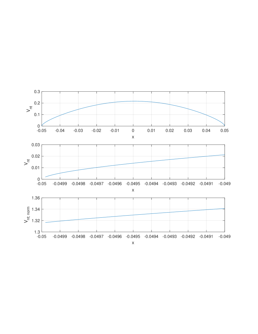
Figure 1. Double no-touch option, $h_{-}=-0.05,h_{+}=0.05$, $T=0.25$, $\nu=1.2,m_{2}=0.1,\lambda_{+}=1,\lambda_{-}=-2,\mu=0$.

In Fig. 1, we show the graph of a no-touch option as a function of $x\in[-0.04998,0.04998]$, at 4,999 points. $X$ is KoBoL of order $\nu=1.2$, $\mu=0$, $\lambda_{+}=1,\lambda_{-}=-2$, $c=c_{+}=c_{-}$ is defined from $m_{2}:=\psi^{\prime\prime}(0)=0.1$. Precision E-14 is achieved in 11.0 sec. if the sinh-acceleration is used.

The upper panel: graph for $x\in(h_{-},h_{+})$. The middle panel: graph in a small vicinity of $h_{-}$. The lower panel: price shown in the middle panel is normalized by $(x-h_{-})^{\nu/2}$. As it is proved in [8] in the case of single barrier options, in the case $\nu>1$ and in the case $\nu\in(0,1),\mu=0$, the price $V(x)$ has the asymptotics $V(x)\sim A(x-h_{-})^{\nu/2}$ as $x\downarrow h_{-}$. Using the standard localization results for boundary problems for elliptic [31] and quasi-elliptic (in particular, parabolic) pseudo-differential operators [43, 46], it is possible to prove that the asymptotics of the same form is valid for barrier options with two barriers (although, contrary to [8], an explicit formula for the asymptotic coefficient $A$ is impossible to derive). Numerical examples in [8] demonstrate that the asymptotic formula is moderately accurate in a very small vicinity of the barrier only, and the quality of approximation decreases as $\nu$ approaches either 0 or 1. The presence of the second barrier decreases the accuracy of the asymptotic approximation further still but, as the lower panel demonstrates, the relative error of the asymptotic formula is of the order of 10%.

Example 5.2.

In Fig. 2, we show the graph of the double barrier digital as a function of $(x,a)\in[-0.049,0.049]^{2}$, at $99^{2}=9,981$ points. $T=0.25,h_{\pm}=\pm 0.05$. $X$ is KoBoL of order $\nu=1.2$, $\mu=0.02$, $\lambda_{+}=1,\lambda_{-}=-2$, $c=c_{+}=c_{-}$ is defined from $\psi^{\prime\prime}(0)=0.1$. Precision E-14 is achieved in 229 sec, E-7 in 22.6 sec. if the sinh-acceleration is used; if the GWR acceleration is used, then precision better than E-5 is achieved in 11.1 sec.

5.3. Shapes of price curves

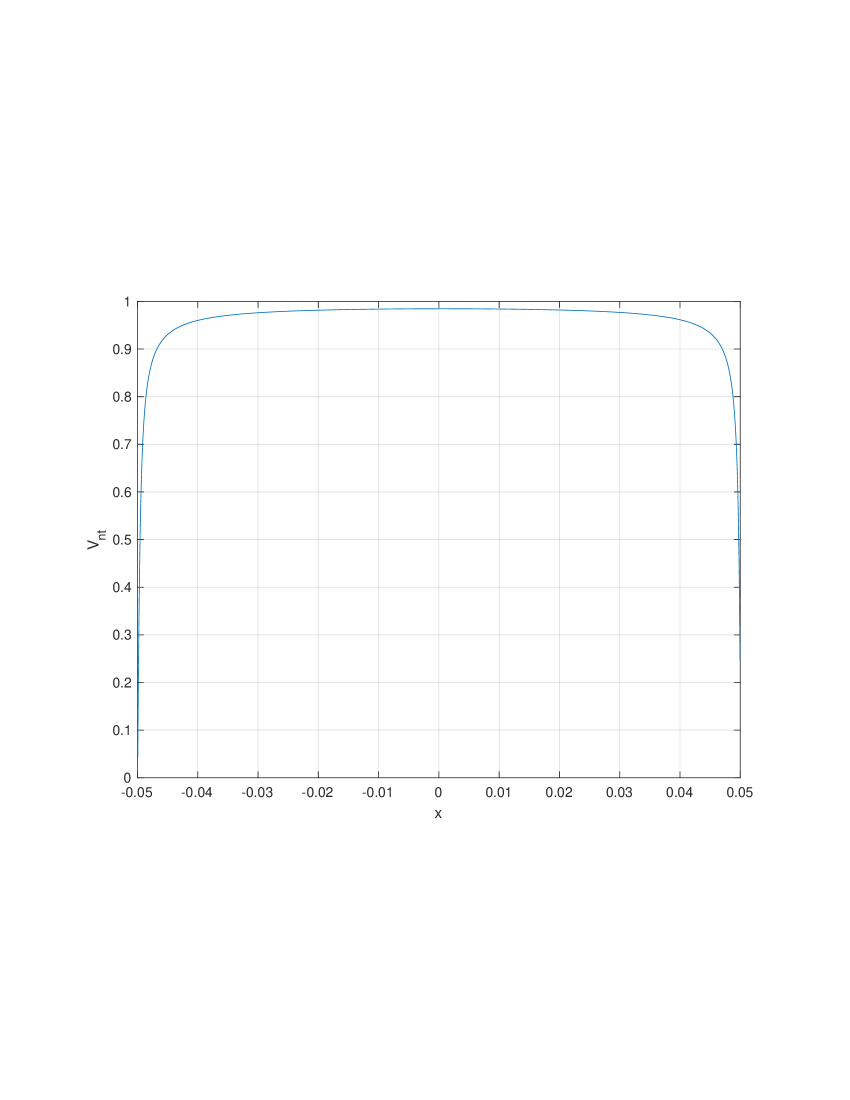
Figure 3. Double barrier no-touch option, $h_{-}=-0.05,h_{+}=0.05$, $T=0.01$, $\nu=0.8,m_{2}=0.1,\lambda_{+}=1,\lambda_{-}=-2,\mu=0$.

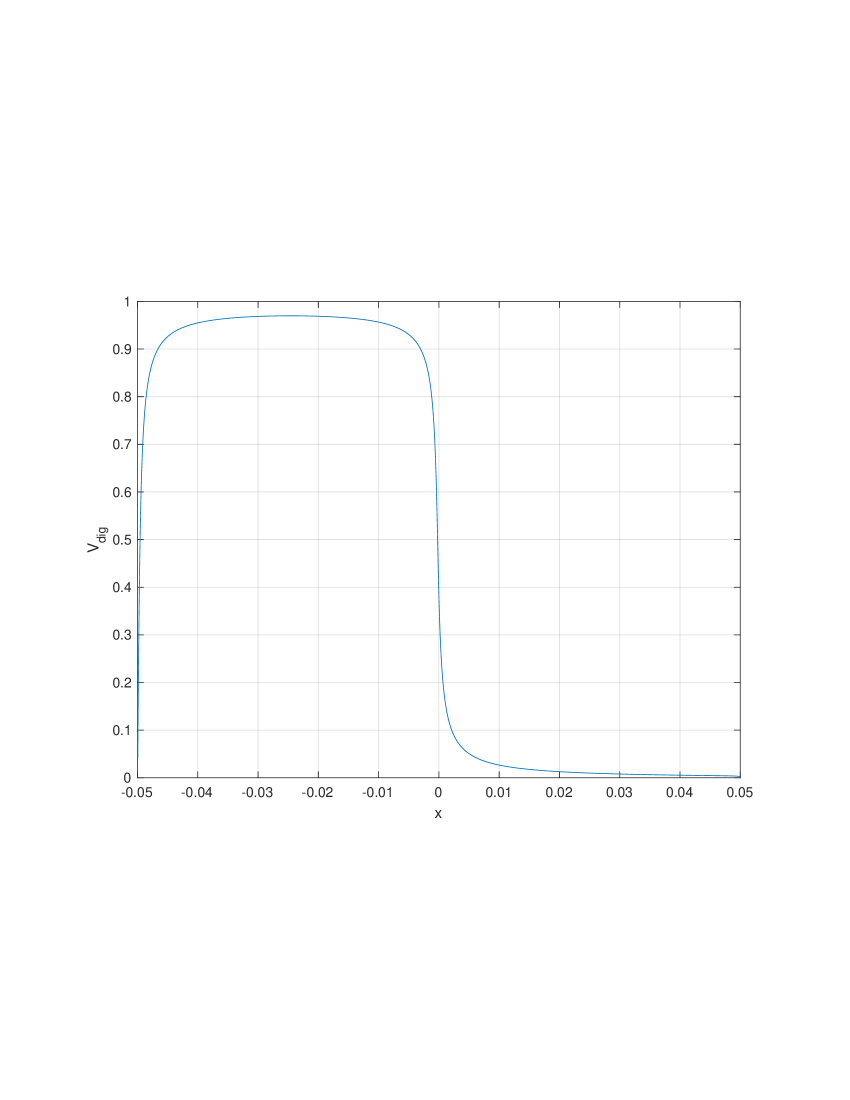
Figure 4. Double barrier digital, $h_{-}=-0.05,h_{+}=0.05$, $T=0.01$, strike $K=e^{0}=1$, $\nu=0.8,m_{2}=0.1,\lambda_{+}=1,\lambda_{-}=-2,\mu=0$.

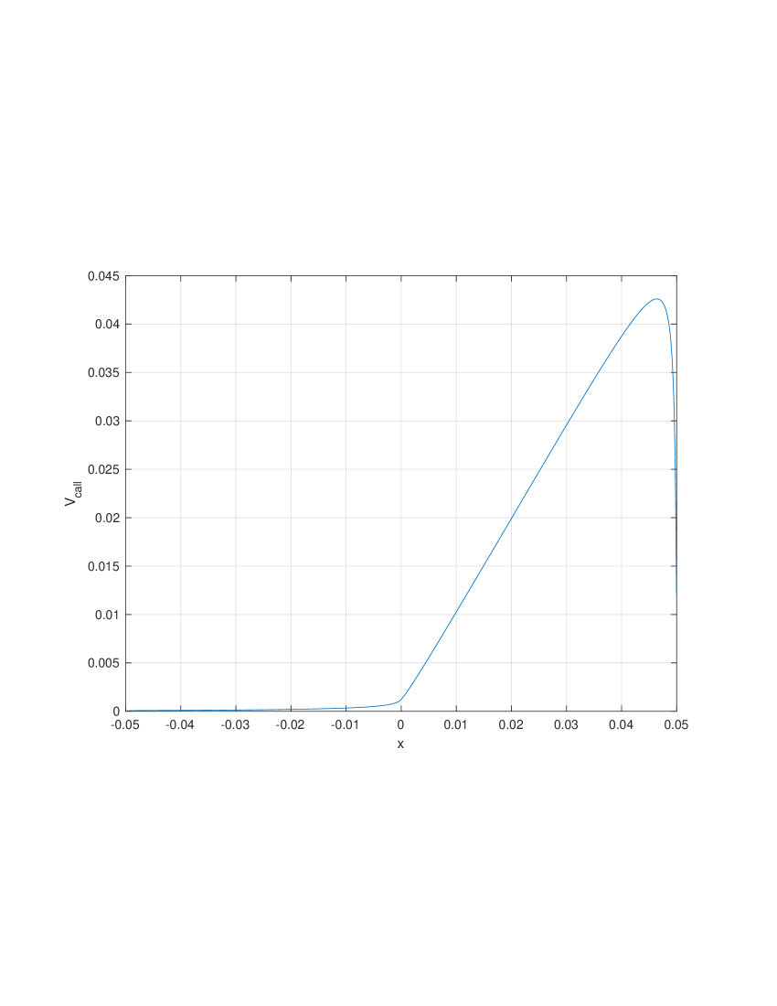
Figure 5. Double barrier call option, $h_{-}=-0.05,h_{+}=0.05$, $T=0.01$, strike $K=e^{0}=1$, $\nu=0.8,m_{2}=0.1,\lambda_{+}=1,\lambda_{-}=-2,\mu=0$.

We plot the price curves of the double barrier no-touch option (Fig. 3) digital (Fig. 4) and call option (Fig. 5) in the exponential Lévy model $S_{t}=e^{X_{t}}$, close to maturity date $T=0.01$; the barriers are $H_{\pm}=e^{h_{\pm}}$, the strike is $K=1=e^{0}$. $X$ is KoBoL of order $\nu=0.8$, $\mu=0.02$, $\lambda_{+}=1,\lambda_{-}=-2$, $c=c_{+}=c_{-}$ is defined from $m_{2}:=\psi^{\prime\prime}(0)=0.1$. Since $\nu<1$ and $\mu>0$, $V(h_{-}+)>0$. This fact is proved in [8] for single barrier options. Using the standard localization results for boundary problems for elliptic [31] and quasi-elliptic (in particular, parabolic) pseudo-differential operators [43, 46], it is possible to prove that $V(h_{-}+)>0$ for barrier options with two barriers, if $\nu<1$ and $\mu>0$. Naturally, in the case of the call option of small maturity, and strike half-way between the barriers, the limit is very small.

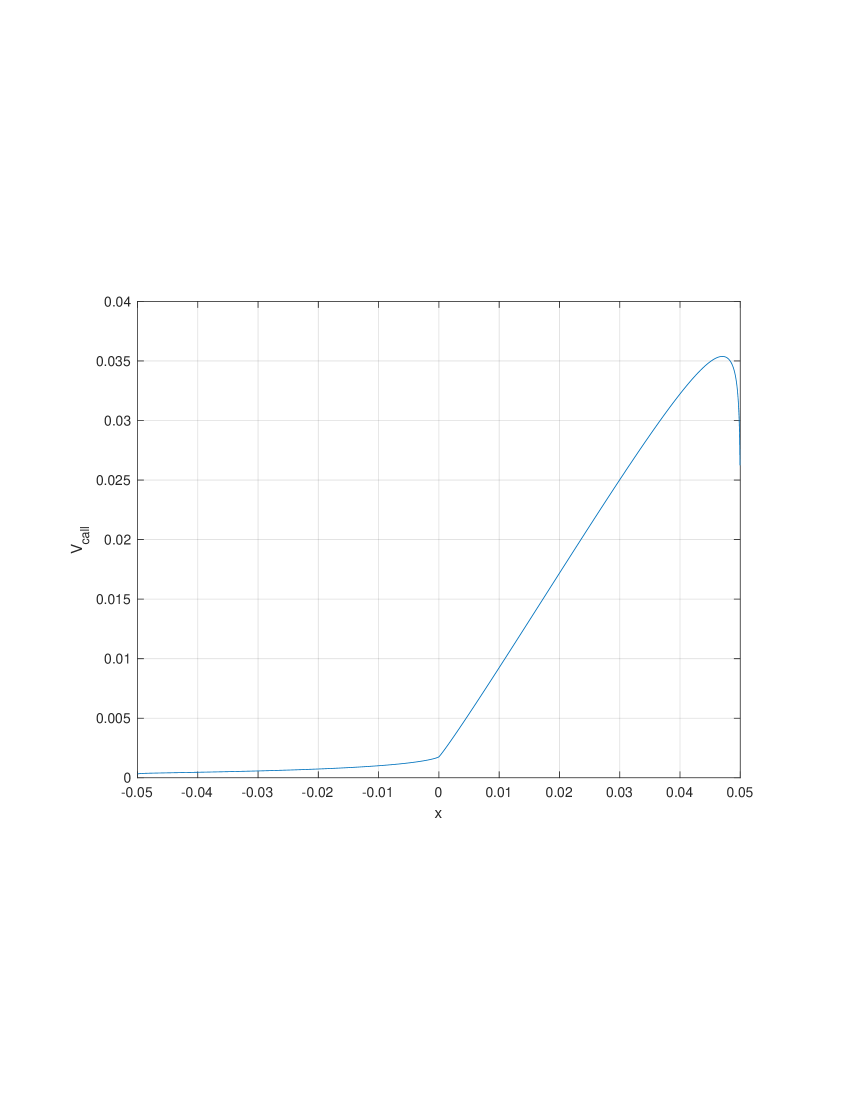
Figure 6. Double barrier call option, $h_{-}=-0.05,h_{+}=0.05$, $T=0.25$, $K=1$, $\nu=0.2,m_{2}=0.1,\lambda_{+}=1,\lambda_{-}=-2,\mu=0$.

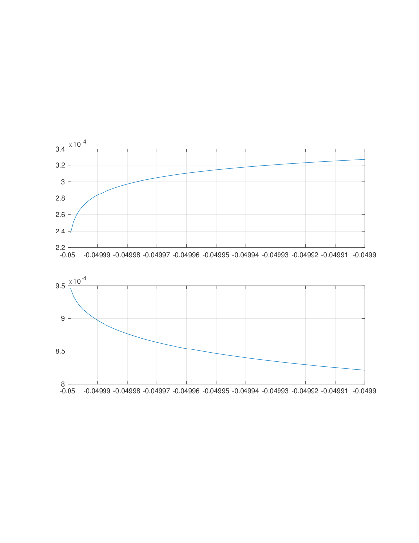
Figure 7. Double barrier call option, $h_{-}=-0.05,h_{+}=0.05$, $T=0.25$, strike $K=e^{0}=1$. $K=1$, $\nu=0.2,m_{2}=0.1,\lambda_{+}=1,\lambda_{-}=-2,\mu=0$. Upper panel; the call price. Lower panel: the normalized price $V_{call;norm}(x)=V_{call}(x)/(x-h_{-})^{\nu/2}$

On the other hand, if the process is close to VG, then, even in the case $\mu=0$, the price may seem to have a positive limit at $h_{-}+$ because for processes close to VG, the impact of large jumps is comparable to the impact of small fluctuations, hence, the Blumenthal 0-1 law manifests itself only very close to the boundary. On Fig. 6-7, we plot the graph of the call option price. The parameters are $T=0.25,K=e^{0}=1,\nu=0.2,m_{2}=0.1,\lambda_{+}=1,\lambda_{-}=-2,\mu=0$, hence, $V(h_{-}+0)=0$. On Fig. 6, where the graph on $[h_{-}+0.001,h_{+}-0.001]$ is plotted, it seems that $V(h_{-}+0)>0$. On Fig. 7, upper panel, we plot the price curve in a small vicinity of $h_{-}$. It is seen that the price started to decrease as $x$ approaches $h_{-}$. The lower panel shows the normalized price $V_{call;norm}(x)=V_{call}(x)/(x-h_{-})^{\nu/2}$.

Clearly, if the price is calculated using the calculations in the state space, backward induction and interpolation at each time step, then, if the linear interpolation is used and $\Delta x\geq 10^{-4}$, where $\Delta x$ is the step of the grid used for the interpolation, the error introduced at each step is of the order of $\Delta x$. Interpolation of higher order may produce huge errors because even the first derivative of the price tends to infinity as the underlying approaches the barrier.

5.4. Tables: dependence of precision on the method for the Laplace inversion, time to maturity and the order of the process

In tables in Section A, the “benchmark values” are the values obtained using the sinh-acceleration with different deformations of the three contours of integration; in all examples, we use the algorithm with Step IX(1) (truncation of the series) and $M_{0}=9$. We calculate the error of the “benchmark values” w.r.t. the values obtained with the scheme with step IX(2) (using the matrix inverse instead of the truncated sum). We stop increasing $T$ when the truncation error becomes larger than E-15, and larger $M_{0}$ are necessary to use to satisfy the error tolerance E=15. If $\nu=1.2$, this happens at $T=1$, if $\nu=0.2$, at $T=3$. We determine where to stop looking at the prices of the call option. If $\nu=0.2$, then the scheme with Step IX(2) achieves accuracy of the order of E-11 at $T=5$; at $T=10$, high precision arithmetic is needed. If $\nu=1.2$, the scheme with Step IX(2) achieves the precision better than E-16 at $T=3$; since the prices are of the order of $E-12$, the relative error is smaller than $E-03$. For $T\leq 1$, the differences are of the order of E-15 or better. If the order $\nu<1$ and drift $\mu\neq 0$, then only the GWR acceleration is applicable.

Remark 5.1.

Some rows of prices may seem wrong. For instance, for $T\leq 3$ in Table 6, the sequences of prices are increasing if $T=0.004,0.25,3$. The reason is that the grid step is 0.01. For $T=0.004,0.25,$ the peak of the price curve is on $(0.04,0.005)$, for $T=3$, the peak is on $(0.03,0.04)$. See Fig. 6 and 8.

6. Conclusion

In the paper, we develop a very fast and accurate method for pricing double barrier options with continuous monitoring in wide classes of Lévy models; the method extends the method developed in [25] for single barrier options and more general options with barrier/lookback features. For each $q$ in the Laplace inversion formula (we use the sinh-acceleration in the Bromwich integrals and the Gaver-Wynn Rho acceleration algorithm), the main block is the evaluation of two series of perpetual first touch options (or their analytic continuation w.r.t. $q$). The iteration procedure for the evaluation of the series in the operator form is the same as in [10], where the calculations are in the state space and the technique of the expected present value operators (EPV-operators) is used. The calculations in the dual space allow for much more efficient calculations. The iteration procedure in the present paper can be applied in a similar vein to double barrier options with discrete monitoring and calculation of joint probability distributions in stable Lévy models. See [27, 26] for the single barrier case. The procedure can be applied to improve the performance of pricing of barrier and American options in regime-switching Lévy models, approximations of models with stochastic volatility and interest rates with regime-switching models, where the technique of the EPV-operators was used [18, 19, 16, 29, 7, 21].

For wide regions in the parameter space, the precision of the order of $10^{-15}$ is achievable in seconds, and of the order of $10^{-9}-10^{-8}$ - in fractions of a second. The Wiener-Hopf factors and repeated integrals in the pricing formulas are calculated using the sinh-deformation of the lines of integration, the corresponding changes of variables and the simplified trapezoid rule. If the Bromwich integral is calculated using the Gaver-Wynn Rho acceleration instead of the sinh-acceleration, the CPU time is typically smaller but the precision is of the order of $10^{-9}-10^{-6}$, at best. Explicit pricing algorithms and numerical examples are for no-touch options, digitals (equivalently, for the joint distribution function of a Lévy process and its supremum and infimum processes), and call options.

We produce several graphs to explain fundamental difficulties for accurate pricing of barrier options using the time discretization or Carr’s randomization and interpolation-based calculations in the state space.

Appendix A Figures and tables

Table 1. Double barrier no-touch option. KoBoL close to NIG, with an almost symmetric jump density, and no “drift”: $m_{2}=0.1,\nu=1.2,\lambda_{-}=-2,\lambda_{+}=1,\mu=0$. Riskless rate $r=0$. Prices and errors (rounded) of the algorithm with the sinh- and GWR-acceleration applied to the Bromwich integral (SINH and GWR). (Log-)barriers: $h_{-}=-0.05,h_{+}=0.05$. Time to maturity $T=0.004,0.25,1$.

$x$	-0.04	-0.02	0	0.02	0.04
$T=0.004$
$V_{nt}$	0.944232464403407	0.984791837906914	0.988695065999628	0.985130282346314	0.945243176095013
$err_{1}$	-4.13E-08	-1.176E-08	-9.88E-09	-1.29E-08 -	-3.951E-08
$err_{2}$	-1.09E-07	6.22E-09	9.06E-09	1.15E-08	-1.12E-07
$T=0.25$
$V_{nt}$	0.0925697509133228	0.183597478719832	0.216239237263554	0.187081211429371	0.0961682820257716
$err_{1}$	1.05E-06	6.87E-08	7.83E-08	6.67E-08	1.03E-06
$err_{2}$	8.49E-06	5.92E-06	5.63E-07	6.22E-06	9.79E-06
$T=1$
$V_{nt}$	0.000488706725350729	0.000970205697557125	0.00114386828643243	0.000989805061225368	0.000508651147353323
$err_{1}$	-2.67E-05	-9.94E-06	-6.30E-06	-1.05E-05	-2.81E-05
$err_{2}$	1.23E-05	1.39E-05	1.01E-05	1.47E-05	1.27E-05

$\underline{T=0.004}$. Benchmark values at 9 points: CPU time 15.2 sec, precision is better than E-15.
Sizes of arrays for the benchmark: $N_{\ell}=417$, $N^{-}=214$, $N^{+}=241$, $N^{\pm}_{1}=1504$.
$\epsilon_{1}$: errors of SINH with $N_{\ell}=112$, $N^{-}=63$, $N^{+}=84$, $N^{\pm}_{1}=298$. CPU time 0.746 sec.
$\epsilon_{2}$: error of GWR with $M=8$, $N^{-}=23$, $N^{+}=38$, $N^{\pm}_{1}=93$. CPU time 0.097 sec.

$\underline{T=0.25}$. Benchmark values at 9 points: CPU time 6.80 sec, precision is better than E-15.
Sizes of arrays for the benchmark: $N_{\ell}=230$, $N^{-}=171$, $N^{+}=182$, $N^{\pm}_{1}=1193$.
$\epsilon_{1}$: errors of SINH with $N_{\ell}=59$, $N^{-}=69$, $N^{+}=79$, $N^{\pm}_{1}=203$. CPU time 0.615 sec.
$\epsilon_{2}$: error of GWR with $M=8$, $N^{-}=136$, $N^{+}=144$, $N^{\pm}_{1}=954$. CPU time 0.375 sec.

$\underline{T=1}$. Benchmark values at 9 points: CPU time 9.17 sec, precision is better than E-15.
Sizes of arrays for the benchmark: $N_{\ell}=215$, $N^{-}=198$, $N^{+}=222$, $N^{\pm}_{1}=1676$.
$\epsilon_{1}$: errors of SINH with $N_{\ell}=29$, $N^{-}=29$, $N^{+}=48$, $N^{\pm}_{1}=117$. CPU time 0.111 sec.
$\epsilon_{2}$: error of GWR with $M=8$, $N^{-}=23$, $N^{+}=38$, $N^{\pm}_{1}=93$. CPU time 0.097 sec.

Table 2. Double barrier no-touch option. KoBoL close to VG, with an almost symmetric jump density, and no drift: $m_{2}=0.1,\nu=0.2,\lambda_{-}=-2,\lambda_{+}=1,\mu=0$. Riskless rate $r=0$. Prices and errors (rounded) of the algorithm with the sinh- and GWR-acceleration applied to the Bromwich integral (SINH and GWR). (Log-)barriers: $h_{-}=-0.05,h_{+}=0.05$. Time to maturity $T=0.004,0.25,3$.

$x$	-0.04	-0.02	0	0.02	0.04
$T=0.004$
$V_{nt}$	0.997159234166403	0.99785039353072	0.997988709856923	0.997873055193352	0.997205955464661
$err_{1}$	2.53E-11	5.77E-11	5.27E-11	3.80E-11	6.86E-11
$err_{2}$	5.13E-10	-8.84E-10	-5.30E-10	4.14E-10	-1.32E-11
$T=0.25$
$V_{nt}$	0.837255746301533	0.872998705974284	0.880407965481731	0.87420738492834	0.83967624398896
$err_{1}$	5.16E-08	5.60E-08	-5.45E-11	2.37E-08	2.23E-08
$err_{2}$	2.43E-08	3.31E-08	2.88E-08	2.75E-08	2.61E-08
$T=3$
$V_{nt}$	0.133264677579268	0.179416477579805	0.192359856627979	0.181619873768539	0.136797832249264
$err_{1}$	-3.33E-08	-2.82E-08	-2.65E-08	-2.70E-08	-3.34E-08
$err_{2}$	2.48E-08	5.42E-08	2.05E-08	1.49E-08	2.25E-09
1.23E-05	1.39E-05	1.01E-05	1.47E-05	1.27E-05

$\underline{T=0.004}$. Benchmark values at 9 points: CPU time 9.83 sec, precision is better than E-15.
Sizes of arrays for the benchmark: $N_{\ell}=356$, $N^{-}=164$, $N^{+}=174$, $N^{\pm}_{1}=1254$.
$\epsilon_{1}$: errors of SINH with $N_{\ell}=171$, $N^{-}=73$, $N^{+}=92$, $N^{\pm}_{1}=379$. CPU time 2.037 sec.
$\epsilon_{2}$: error of GWR with $M=8$, $N^{-}=59$, $N^{+}=75$, $N^{\pm}_{1}=311$. CPU time 0.171 sec.

$\underline{T=0.25}$. Benchmark values at 9 points: CPU time 6.50 sec, precision is better than E-15.
Sizes of arrays for the benchmark: $N_{\ell}=230$, $N^{-}=177$, $N^{+}=188$, $N^{\pm}_{1}=979$.
$\epsilon_{1}$: errors of SINH with $N_{\ell}=72$, $N^{-}=48$, $N^{+}=67$, $N^{\pm}_{1}=162$. CPU time 0.377 sec.
$\epsilon_{2}$: error of GWR with $M=8$, $N^{-}=136$, $N^{+}=144$, $N^{\pm}_{1}=954$. CPU time 0.402 sec.

$\underline{T=3}$. Benchmark values at 9 points: CPU time 4.45 sec, precision is better than E-15.
Sizes of arrays for the benchmark: $N_{\ell}=152$, $N^{-}=164$, $N^{+}=184$, $N^{\pm}_{1}=1397$.
$\epsilon_{1}$: errors of SINH with $N_{\ell}=34$, $N^{-}=47$, $N^{+}=60$, $N^{\pm}_{1}=190$. CPU time 0.204 sec.
$\epsilon_{2}$: error of GWR with $M=8$, $N^{-}=30$, $N^{+}=40$, $N^{\pm}_{1}=112$. CPU time 0.119 sec.

Table 3. Double barrier digital put. (Log-)barriers: $h_{-}=-0.05,h_{+}=0.05$; log-strike $a=-0.01$. KoBoL close to NIG, with an almost symmetric jump density, and no “drift”: $m_{2}=0.1,\nu=1.2,\lambda_{-}=-2,\lambda_{+}=1,\mu=0$. Riskless rate $r=0$. Prices and errors (rounded) of the algorithm with the sinh- and GWR-acceleration applied to the Bromwich integral (SINH and GWR). Time to maturity $T=0.004,0.25,1$.

$x$	-0.04	-0.02	0	0.02	0.04
$T=0.004$
$V_{dig}$	0.936033131420221	0.942743923266939	0.0407165015135701	0.00756840253469884	0.00309395728748227
$\epsilon_{1}$	6.64E-10	-3.51E-10	3.28E-10	5.08E-10	-6.12E-10
$\epsilon_{2}$	-6.13E-08	5.34E-09	2.57E-09	8.58E-10	2.05E-09
$T=0.25$
$V_{dig}$	0.0367167500936684	0.0706406957622098	0.0786094461300362	0.0641355992734415	0.0319013015638287
$\epsilon_{1}$	1.48E-07	3.23E-08	1.88E-08	1.36E-08	1.08E-08
$\epsilon_{2}$	-9.39E-07	1.27E-06	-6.34E-06	-1.97E-06	-1.83E-06
$T=1$
$V_{dig}$	0.000177771957381001	0.000352921137775741	0.000416090671743419	0.000360047453580148	0.000185024416500812
$\epsilon_{1}$	1.07E-07	1.32E-07	6.97E-08	4.12E-08	2.85E-08
$\epsilon_{2}$	-1.73E-05	-6.21E-06	8.72E-07	9.36E-06	8.59E-06

$\underline{T=0.004}$. Benchmark values at 9 points: CPU time 13.8 sec, precision is better than E-15.
Sizes of arrays for the benchmark: $N_{\ell}=449$, $N^{-}=177$, $N^{+}=197$, $N^{\pm}_{1}=1088$.

$\epsilon_{1}$: errors of SINH with $N_{\ell}=158$, $N^{-}=49$, $N^{+}=76$, $N^{\pm}_{1}=184$. CPU time 1.00 sec.
$\epsilon_{2}$: error of GWR with $M=8$, $N^{-}=82$, $N^{+}=99$, $N^{\pm}_{1}=387$. CPU time 0.237 sec. $\underline{T=0.25}$. Benchmark values at 9 points: CPU time 8.81 sec, precision is better than E-15.
Sizes of arrays for the benchmark: $N_{\ell}=305$, $N^{-}=167$, $N^{+}=178$, $N^{\pm}_{1}=1891$.

$\epsilon_{1}$: errors of SINH with $N_{\ell}=86$, $N^{-}=46$, $N^{+}=65$, $N^{\pm}_{1}=152$. CPU time 0.413 sec.
$\epsilon_{2}$: error of GWR with $M=8$, $N^{-}=136$, $N^{+}=144$, $N^{\pm}_{1}=731$. CPU time 0.399 sec. $\underline{T=1}$. Benchmark values at 9 points: CPU time 9.29 sec, precision is better than E-15.
Sizes of arrays for the benchmark: $N_{\ell}=259$, $N^{-}=200$, $N^{+}=241$, $N^{\pm}_{1}=1410$.

$\epsilon_{1}$: errors of SINH with $N_{\ell}=51$, $N^{-}=43$, $N^{+}=69$, $N^{\pm}_{1}=157$. CPU time 0.267 sec.
$\epsilon_{2}$: error of GWR with $M=8$, $N^{-}=84$, $N^{+}=110$, $N^{\pm}_{1}=422$. CPU time 0.273 sec.

Table 4. Double barrier digital put. (Log-)barriers: $h_{-}=-0.05,h_{+}=0.05$; log-strike $a=-0.01$. KoBoL close to VG, with an almost symmetric jump density, and no “drift”: $m_{2}=0.1,\nu=0.2,\lambda_{-}=-2,\lambda_{+}=1,\mu=0$. Riskless rate $r=0$. Prices and errors (rounded) of the algorithm with the sinh- and GWR-acceleration applied to the Bromwich integral (SINH and GWR). Time to maturity $T=0.004,0.25,3$.

$x$	-0.04	-0.02	0	0.02	0.04
$T=0.004$
$V_{dig}$	0.996564411171869	0.99657921660561	0.00112224938146623	0.000499111365249944	0.00031397891513379
$\epsilon_{1}$	6.64E-10	-3.51E-10	3.28E-10	5.08E-10	-6.12E-10
$\epsilon_{2}$	-1.81E-10	-1.23E-10	5.16E-11	2.89E-11	-3.29E-14
$T=0.25$
$V_{dig}$	0.806048752314656	0.808342339586413	0.0564741685789332	0.0263104606596591	0.0165845924903516
$\epsilon_{1}$	3.56E-08	2.30E-08	1.86E-08	1.53E-08	1.28E-08
$\epsilon_{2}$	3.57E-08	1.618E-08	7.169E-09	3.163E-08	2.758E-08
$T=3$
$V_{dig}$	0.0826482000571708	0.0963948765801401	0.064756560941078	0.0445502961594203	0.0292378743031199
$\epsilon_{1}$	7.40E-08	4.54E-08	4.136E-08	1.99E-08	3.347E-08
$\epsilon_{2}$	-9.69E-07	4.54E-07	8.08E-08	-3.42E-07	-1.72E-08

$\underline{T=0.004}$. Benchmark values at 9 points: CPU time 6.92 sec, precision is better than E-15.
Sizes of arrays for the benchmark: $N_{\ell}=230$, $N^{-}=165$, $N^{+}=199$, $N^{\pm}_{1}=1175$.
$\epsilon_{1}$: errors of SINH with $N_{\ell}=143$, $N^{-}=51$, $N^{+}=69$, $N^{\pm}_{1}=178$. CPU time 0.861sec.
$\epsilon_{2}$: error of GWR with $M=8$, $N^{-}=69$, $N^{+}=91$, $N^{\pm}_{1}=362$. CPU time 0.290 sec. $\underline{T=0.25}$. Benchmark values at 9 points: CPU time 8.81 sec, precision is better than E-15.
Sizes of arrays for the benchmark: $N_{\ell}=230$, $N^{-}=165$, $N^{+}=199$, $N^{\pm}_{1}=117$.

$\epsilon_{1}$: errors of SINH with $N_{\ell}=72$, $N^{-}=50$, $N^{+}=75$, $N^{\pm}_{1}=193$. CPU time 0.414 sec.
$\epsilon_{2}$: error of GWR with $M=8$, $N^{-}=32$, $N^{+}=51$, $N^{\pm}_{1}=731$. CPU time 0.075 sec.

$\underline{T=3}$. Benchmark values at 9 points: CPU time 5.56 sec, precision is better than E-15.
Sizes of arrays for the benchmark: $N_{\ell}=164$, $N^{-}=189$, $N^{+}=213$, $N^{\pm}_{1}=1950$.

$\epsilon_{1}$: errors of SINH with $N_{\ell}=27$, $N^{-}=43$, $N^{+}=56$, $N^{\pm}_{1}=183$. CPU time 0.145 sec.
$\epsilon_{2}$: error of GWR with $M=8$, $N^{-}=51$, $N^{+}=67$, $N^{\pm}_{1}=309$. CPU time 0.143 sec.

Table 5. Double barrier call. (Log-)barriers: $h_{-}=-0.05,h_{+}=0.05$; log-strike $a=0$. KoBoL close to NIG, with an almost symmetric jump density, and no “drift”: $m_{2}=0.1,\nu=1.2,\lambda_{-}=-2,\lambda_{+}=1,\mu=0$. Riskless rate $r=0$. Prices and errors (rounded) of the algorithm with the sinh- and GWR-acceleration applied to the Bromwich integral (SINH and GWR). Time to maturity $T=0.004,0.25,1,3$.

$x$	-0.04	-0.02	0	0.02	0.04
$T=0.004$
$V_{call}$	0.0000824404624213168	0.000204166217898571	0.00191177395953069	0.0197639609828199	0.0376099511198009
$\epsilon_{1}$	-3.88E-10	-5.43E-10	-7.59E-10	-1.25E-09	-3.68E-09
$\epsilon_{2}$	3.48E-11	-5.23E-10	4.67E-10	5.85E-10	-5.81E-09
$T=0.25$
$V_{call}$	0.00082409621567	0.00169255391432158	0.00212237950197215	0.00195192815759268	0.0010370403093618
$\epsilon_{1}$	-2.24E-07	-3.00E-07	-5.51E-07	-4.50E-07	-4.68E-07
$\epsilon_{2}$	-1.92E-07	-2.02E-07	-4.01E-07	-2.26E-07	-1.29E-07
$T=1$
$V_{call}$	4.80103589597936E-06	9.53128787591073E-06	0.0000112373996155185	9.72392418717438E-06	4.99704769890697E-06
$\epsilon_{1}$	5.93E-11	7.07E-11	1.09E-10	2.40E-10	5.45E-10
$\epsilon_{2}$	4.41E-06	7.80E-06	7.86E-06	5.65E-06	2.50E-06
$\epsilon_{3}$	6.43E-13	9.80E-13	1.64E-12	3.09E-12	7.31E-12
$T=3$
$V_{call}$	4.074629523	8.089334758	9.537398649	8.252398764	4.240829909
$\epsilon$	1.67E-16	-5.55E-17	-2.78E-17	2.78E-16	-4.44E-16
$rel_{\epsilon}$	1.39E-04	-8.33E-05	-2.78E-05	3.05E-04	-3.61E-04

$T=0.004$. Benchmark values at 9 points: CPU time 14.5 sec, precision is better than E-16.
Sizes of arrays for the benchmark: $N_{\ell}=464$, $N^{-}=180$, $N^{+}=193$, $N^{\pm}_{1}=1410$.
$\epsilon_{1}$: errors of SINH with $N_{\ell}=109$, $N^{-}=73$, $N^{+}=89$, $N^{\pm}_{1}=272$. CPU time 1.30 sec.
$\epsilon_{2}$: error of GWR with $M=8$, $N^{-}=58$, $N^{+}=78$, $N^{\pm}_{1}=349$. CPU time 0.128 sec. $T=0.25$. Benchmark values at 9 points: CPU time 8.81 sec, precision is better than E-15.
Sizes of arrays for the benchmark: $N_{\ell}=254$, $N^{-}=175$, $N^{+}=188$, $N^{\pm}_{1}=1376$.
$\epsilon_{1}$: errors of SINH with $N_{\ell}=16$, $N^{-}=27$, $N^{+}=33$, $N^{\pm}_{1}=71$. CPU time 0.073 sec.
$\epsilon_{2}$: errors of GWR with $M=8$, $N^{-}=31$, $N^{+}=44$, $N^{\pm}_{1}=126$. CPU time 0.072 sec.

$T=1$. “Benchmark values” (BB values) at 9 points: CPU time 9.82 sec, precision is better than E-15 if schemes with different deformations but the same $M_{0}=9$ are compared .
Sizes of arrays for the benchmark: $N_{\ell}=276$, $N^{-}=208$, $N^{+}=222$, $N^{\pm}_{1}=1312$.
$\epsilon_{1}$: errors of SINH with $N_{\ell}=59$, $N^{-}=50$, $N^{+}=66$, $N^{\pm}_{1}=968$. CPU time 0.317 sec.
$\epsilon_{2}$: errors of GWR with $M=8$, $N^{-}=152$, $N^{+}=162$, $N^{\pm}_{1}=126$. CPU time 0.521 sec.
$\epsilon_{3}$: errors of BB values w.r.t. to the scheme using IX(2) (matrix inversion instead of truncation of the series). $T=3$. Values ($V_{call}$) in units of $10^{-12}$, differences (in units of 1) and relative differences between values calculated using different deformations ($\epsilon$ and $rel_{\epsilon}$); step IX(2) is used.
Errors of GWR and Step IX(1) with any $M_{0}$ (and double precision arithmetic) are of the order of the values.

Table 6. Double barrier call. (Log-)barriers: $h_{-}=-0.05,h_{+}=0.05$; log-strike $a=0$. KoBoL close to VG, with an almost symmetric jump density, and no “drift”: $m_{2}=0.1,\nu=0.2,\lambda_{-}=-2,\lambda_{+}=1,\mu=0$. Riskless rate $r=0$. Prices and errors (rounded) of the algorithm with the sinh- and GWR-acceleration applied to the Bromwich integral (SINH and GWR). Time to maturity $T=0.004,0.25,3,5$.

$x$	-0.04	-0.02	0	0.02	0.04
$T=0.004$
$V_{call}$	8.77581627294074E-06	0.0000140126705130402	0.0000365669756568704	0.0201495491781489	0.0406572530052907
$\epsilon_{1}$	1.88E-10	3.45E-11	-3.96E-10	3.207E-12	-3.87E-10
$\epsilon_{2}$	-1.45E-10	2.00E-10	4.10E-10	4.56E-10	1.02E-09
$T=0.25$
$V_{call}$	0.000461949526934386	0.000737018983172683	0.001757476257127	0.0171789730510928	0.032229359938136
$\epsilon_{1}$	-3.62E-10	-5.38E-10	-8.39E-10	-6.50E-10	-1.15E-09
$\epsilon_{2}$	-6.14E-09	5.54E-09	9.84E-09	-5.37E-09	-5.705E-09
$T=3$
$V_{call}$	0.00080243923836716	0.00124070584073691	0.00182400986139031	0.00268682684255628	0.00274066739944123
$\epsilon_{1}$	-6.20E-08	-6.93E-08	-7.87E-08	-9.20E-08	-1.17E-07
$\epsilon_{2}$	1.11E-08	4.56E-08	-1.90E-07	-9.07E-08	-1.388E-07
$T=5$
$V_{call}$	0.000327733526265667	0.000493515765859709	0.000630026253687271	0.000720082418558615	0.000595670818077265
$\epsilon$	5.61E-12	5.70E-12	5.802E-12	5.90E-12	6.00E-12

$T=0.004$. Benchmark values at 9 points: CPU time 19.1 sec, precision is better than E-16.
Sizes of arrays for the benchmark: $N_{\ell}=649$, $N^{-}=173$, $N^{+}=186$, $N^{\pm}_{1}=1175$.

$\epsilon_{1}$: errors of SINH with $N_{\ell}=127$, $N^{-}=54$, $N^{+}=65$, $N^{\pm}_{1}=178$. CPU time 0.749 sec.
$\epsilon_{2}$: error of GWR with $M=8$, $N^{-}=52$, $N^{+}=68$, $N^{\pm}_{1}=207$. CPU time 0.113 sec. $T=0.25$. Benchmark values at 9 points: CPU time 7.63 sec, precision is better than E-16.
Sizes of arrays for the benchmark: $N_{\ell}=255$, $N^{-}=173$, $N^{+}=186$, $N^{\pm}_{1}=1175$.
$\epsilon_{1}$: errors of SINH with $N_{\ell}=79$, $N^{-}=54$, $N^{+}=65$, $N^{\pm}_{1}=178$. CPU time 0.449 sec.

$\epsilon_{2}$: error of GWR with $M=8$, $N^{-}=31$, $N^{+}=44$, $N^{\pm}_{1}=126$. CPU time 0.066 sec.

$T=3$. Benchmark values at 9 points: CPU time 9.82 sec, precision is better than E-15. Errors of BB values w.r.t. to the scheme using IX(2) (matrix inversion instead of truncation of the series) are marginally larger than E-15 at some points, and smaller than E-15 at other points. Sizes of arrays for the benchmark: $N_{\ell}=182$, $N^{-}=173$, $N^{+}=186$, $N^{\pm}_{1}=1175$.
$\epsilon_{1}$: errors of SINH with $N_{\ell}=49$, $N^{-}=59$, $N^{+}=75$, $N^{\pm}_{1}=233$. CPU time 0.316 sec.
$\epsilon_{2}$: error of GWR with $M=8$, $N^{-}=38$, $N^{+}=51$, $N^{\pm}_{1}=143$. CPU time 0.096 sec. $T=5$. Values ($V_{call}$) and differences between values calculated using different deformations ($\epsilon$); Step IX(2) is used. If GWR with Step IX(2) is used, the errors are of the order of E-07.
Errors of GWR and Step IX(1) with any $M_{0}$ (and double precision arithmetic) are of the order of the values.

Figure 2. Double barrier digital, $h_{-}=-0.05,h_{+}=0.05$, $T=0.25$, $\nu=1.2,m_{2}=0.1,\lambda_{+}=1,\lambda_{-}=-2,\mu=0$.

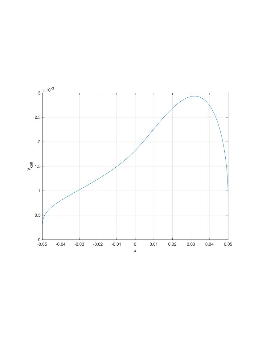
Figure 8. Double barrier call option, $h_{-}=-0.05,h_{+}=0.05$, $T=3$, $K=1$, $\nu=0.2,m_{2}=0.1,\lambda_{+}=1,\lambda_{-}=-2,\mu=0$.

References

- [1] J. Abate and P.P. Valko. Multi-precision Laplace inversion. International Journal of Numerical Methods in Engineering, 60:979–993, 2004.
- [2] J. Abate and W. Whitt. The Fourier-series method for inverting transforms of probability distributions. Queueing Systems, 10:5–88, 1992.
- [3] J. Abate and W. Whitt. Numerical inversion of of probability generating functions. Operation Research Letters, 12:245–251, 1992.
- [4] J. Abate and W. Whitt. A unified framework for numerically inverting Laplace transforms. INFORMS Journal on Computing, 18(4):408–421, 2006.
- [5] S. Asmussen, F. Avram, and M.R. Pistorius. Russian and American put options under exponential phase-type Lévy models. Stochastic Processes and their Applications, 109(1):79–111, 2004.
- [6] F. Avram, A. Kyprianou, and M.R. Pistorius. Exit problems for spectrally negative Lévy processes and applications to (Canadized) Russian options. Annals of Applied Probability, 14(2):215–238, 2004.
- [7] M. Boyarchenko and S. Boyarchenko. Double barrier options in regime-switching hyper-exponential jump-diffusion models. International Journal of Theoretical and Applied Finance, 14(7):1005–1044, 2011.
- [8] M. Boyarchenko, M. de Innocentis, and S. Levendorskiĭ. Prices of barrier and first-touch digital options in Lévy-driven models, near barrier. International Journal of Theoretical and Applied Finance, 14(7):1045–1090, 2011. Available at SSRN: http://papers.ssrn.com/abstract=1514025.
- [9] M. Boyarchenko and S. Levendorskiĭ. Prices and sensitivities of barrier and first-touch digital options in Lévy-driven models. International Journal of Theoretical and Applied Finance, 12(8):1125–1170, December 2009.
- [10] M. Boyarchenko and S. Levendorskiĭ. Valuation of continuously monitored double barrier options and related securities. Mathematical Finance, 22(3):419–444, July 2012.
- [11] S. Boyarchenko and S. Levendorskiĭ. Generalizations of the Black-Scholes equation for truncated Lévy processes. Working Paper, University of Pennsylvania, April 1999.
- [12] S. Boyarchenko and S. Levendorskiĭ. Option pricing for truncated Lévy processes. International Journal of Theoretical and Applied Finance, 3(3):549–552, July 2000.
- [13] S. Boyarchenko and S. Levendorskiĭ. Barrier options and touch-and-out options under regular Lévy processes of exponential type. Annals of Applied Probability, 12(4):1261–1298, 2002.
- [14] S. Boyarchenko and S. Levendorskiĭ. Non-Gaussian Merton-Black-Scholes Theory, volume 9 of Adv. Ser. Stat. Sci. Appl. Probab. World Scientific Publishing Co., River Edge, NJ, 2002.
- [15] S. Boyarchenko and S. Levendorskiĭ. Perpetual American options under Lévy processes. SIAM Journal on Control and Optimization, 40(6):1663–1696, 2002.
- [16] S. Boyarchenko and S. Levendorskiĭ. American options in Lévy models with stochastic volatility, 2007. Available at SSRN: http://ssrn.com/abstract=1031280.
- [17] S. Boyarchenko and S. Levendorskiĭ. Irreversible Decisions Under Uncertainty (Optimal Stopping Made Easy). Springer, Berlin, 2007.
- [18] S. Boyarchenko and S. Levendorskiĭ. Exit problems in regime-switching models. Journ. of Mathematical Economics, 44(2):180–206, 2008.
- [19] S. Boyarchenko and S. Levendorskiĭ. American options in Lévy models with stochastic interest rates. Journal of Computational Finance, 12(4):1–30, Summer 2009.
- [20] S. Boyarchenko and S. Levendorskiĭ. Efficient Laplace inversion, Wiener-Hopf factorization and pricing lookbacks. International Journal of Theoretical and Applied Finance, 16(3):1350011 (40 pages), 2013. Available at SSRN: http://ssrn.com/abstract=1979227.
- [21] S. Boyarchenko and S. Levendorskiĭ. Efficient pricing barrier options and CDS in Lévy models with stochastic interest rate. Mathematical Finance, 27(4):1089–1123, 2017. DOI: 10.1111/mafi.12121.
- [22] S. Boyarchenko and S. Levendorskiĭ. Sinh-acceleration: Efficient evaluation of probability distributions, option pricing, and Monte-Carlo simulations. International Journal of Theoretical and Applied Finance, 22(3), 2019. DOI: 10.1142/S0219024919500110. Available at SSRN: https://ssrn.com/abstract=3129881 or http://dx.doi.org/10.2139/ssrn.3129881.
- [23] S. Boyarchenko and S. Levendorskiĭ. Conformal accelerations method and efficient evaluation of stable distributions. Acta Applicandae Mathematicae, 169:711–765, 2020. Available at SSRN: https://ssrn.com/abstract=3206696 or http://dx.doi.org/10.2139/ssrn.3206696.
- [24] S. Boyarchenko and S. Levendorskiĭ. Static and semi-static hedging as contrarian or conformist bets. Mathematical Finance, 3(30):921–960, 2020. Available at SSRN: https://ssrn.com/abstract=3329694 or http://arxiv.org/abs/1902.02854.
- [25] S. Boyarchenko and S. Levendorskiĭ. Efficient evaluation of expectations of functions of a lévy process and its extremum. Working paper, June 2022. Available at SSRN: https://ssrn.com/abstract=4140462 or http://arXiv.org/abs/4362928.
- [26] S. Boyarchenko and S. Levendorskiĭ. Efficient evaluation of expectations of functions of a stable lévy process and its extremum. Working paper, June 2022. Available at SSRN: http://ssrn.com/abstract=4229032 or http://arxiv.org/abs/2209.12349.
- [27] S. Boyarchenko and S. Levendorskiĭ. Efficient inverse -transform and pricing barrier and lookback options with discrete monitoring. Working paper, June 2022. Available at SSRN: https://ssrn.com/abstract=4155587 or https://doi.org/10.48550/arXiv.2207.02858.
- [28] S. Boyarchenko and S. Levendorskiĭ. Lévy models amenable to efficient calculations. Working paper, June 2022. Available at SSRN: https://ssrn.com/abstract=4116959 or http://arXiv.org/abs/4339862.
- [29] S. Boyarchenko and S.Levendorskiĭ. American options in the Heston model with stochastic interest rate and its generalizations. Appl. Mathem. Finance, 20(1):26–49, 2013.
- [30] P. Carr, H. Geman, D.B. Madan, and M. Yor. The fine structure of asset returns: an empirical investigation. Journal of Business, 75:305–332, 2002.
- [31] G.I. Eskin. Boundary Value Problems for Elliptic Pseudodifferential Equations, volume 9 of Transl. Math. Monogr. American Mathematical Society, Providence, RI, 1981.
- [32] M.V. Fedoryuk. Asymptotic: Integrals and Series. Nauka, Moscow, 1987. In Russian.
- [33] L. Feng and V. Linetsky. Computing exponential moments of the discrete maximum of a Lévy process and lookback options. Finance and Stochastics, 13(4):501–529, 2009.
- [34] G. Fusai, G. Germano, and D. Marazzina. Spitzer identity, Wiener-Hopf factorization and pricing of discretely monitored exotic options. European Journal of Operational Research, 251(1):124–134, 2016. DOI:10.1016/j.ejor.2015.11.027.
- [35] X. Guo and L.A. Shepp. Some optimal stopping problems with nontrivial boundaries for pricing exotic options. J.Appl. Probability, 38(3):647–658, 2001.
- [36] G.G. Haislip and V.K. Kaishev. Lookback option pricing using the Fourier transform B-spline method. Quantitative Finance, 14(5):789–803, 2014.
- [37] J.L. Kirkby. American and Exotic Option Pricing with Jump Diffusions and other Lévy processes. Journ. Comp. Fin., 22(3):13–47, 2018.
- [38] I. Koponen. Analytic approach to the problem of convergence of truncated Lévy flights towards the Gaussian stochastic process. Physics Review E, 52:1197–1199, 1995.
- [39] S.G. Kou. A jump-diffusion model for option pricing. Management Science, 48(8):1086–1101, August 2002.
- [40] S.G. Kou and H. Wang. First passage times of a jump diffusion process. Adv. Appl. Prob., 35(2):504–531, 2003.
- [41] O. Kudryavtsev and S.Z. Levendorskiĭ. Efficient pricing options with barrier and lookback features under Lévy processes. Working paper, June 2011. Available at SSRN: 1857943.
- [42] A. Kuznetsov. Wiener-Hopf factorization and distribution of extrema for a family of Lévy processes. Ann.Appl.Prob., 20(5):1801–1830, 2010.
- [43] S. Levendorskiĭ. Degenerate Elliptic Equations, volume 258 of Mathematics and its Applications. Kluwer Academic Publishers Group, Dordrecht, 1993.
- [44] S. Levendorskiĭ. Pricing of the American put under Lévy processes. International Journal of Theoretical and Applied Finance, 7(3):303–335, May 2004.
- [45] S. Levendorskiĭ. Method of paired contours and pricing barrier options and CDS of long maturities. International Journal of Theoretical and Applied Finance, 17(5):1–58, 2014. 1450033 (58 pages).
- [46] S. Levendorskiĭ and B. Paneyakh. Degenerate elliptic equations and boundary value problems. In M.S. Agranovich and M.A. Shubin, editors, Encyclopeadia of Mathematical Sciences, Vol.63, pages 131–202. Springer, Berlin, 1994.
- [47] L. Li and V. Linetsky. Discretely monitored first passage problems and barrier options: an eigenfunction expansion approach. Finance and Stochastics, 19(3):941–977, 2015.
- [48] V. Linetsky. Spectral methods in derivatives pricing. In J.R. Birge and V. Linetsky, editors, Handbooks in OR & MS, Vol. 15, pages 223–300. Elsevier, New York, 2008.
- [49] F. Stenger. Numerical Methods based on Sinc and Analytic functions. Springer-Verlag, New York, 1993.
- [50] A. Talbot. The accurate inversion of Laplace transforms. J.Inst.Math.Appl., 23:97–120, 1979.
- [51] P.P. Valko and J. Abate. Comparison of sequence accelerators for the Gaver Method of Numerical Laplace Transform inversion. Computers and Mathematics with Applications, 48:629–636, 2004.