Abstract

Visible matter is characterised by a single mass scale; namely, the proton mass. The proton’s existence and structure are supposed to be described by quantum chromodynamics (QCD); yet, absent Higgs boson couplings, chromodynamics is scale invariant. Thus, if the Standard Model is truly a part of the theory of Nature, then the proton mass is an emergent feature of QCD; and emergent hadron mass (EHM) must provide the basic link between theory and observation. Nonperturbative tools are necessary if such connections are to be made; and in this context, we sketch recent progress in the application of continuum Schwinger function methods to an array of related problems in hadron and particle physics. Special emphasis is given to the three pillars of EHM – namely, the running gluon mass, process-independent effective charge, and running quark mass; their role in stabilising QCD; and their measurable expressions in a diverse array of observables.

6 1 0 2022 Nov 21 2022 Dec 18 2022 Dec 19 2023 Jan 11 https://doi.org/10.3390/particles6010004  
Preprint no. NJU-INP 066/22
Emergence of Hadron Mass and Structure Emergence of Hadron Mass and Structure Minghui Ding ^1,‡, Craig D. Roberts ^2,3,‡ and Sebastian M. Schmidt ^1,4,‡ * Minghui Ding, Craig D. Roberts and Sebastian M. Schmidt Ding, M.; Roberts, C.D.; Schmidt, S.M. Correspondence:
  m.ding@hzdr.de (M. Ding); cdroberts@nju.edu.cn (C. D. Roberts); s.schmidt@hzdr.de (S. M. Schmidt) These authors contributed equally to this work.

1 Introduction

Our Universe exists; and even the small part that we occupy contains much which might be considered miraculous. Nevertheless, science typically assumes that the Universe’s evolution can be explained by some collection of equations – even a single equation, perhaps, which replaces distinct theories of many things with a single theory of everything. Choosing not to approach that frontier, then, within the current paradigm, the Standard Model of particle physics (SM) is given a central role; and it must account for a huge array of observable phenomena. Herein, we focus on one especially important aspect, viz. the fact that the mass of the vast bulk of visible material in the Universe is explained as soon as one understands why the proton is absolutely stable and how it comes to possess a mass $m_{p}\approx 1\,$GeV. In elucidating this connection, we will argue that the theory of strong interactions may deliver far more than was originally asked of it.

We have evidently supposed that quantum gauge field theory is the correct paradigm for understanding Nature. In this connection, it is important to note that, in our tangible Universe, time and space give us four noncompact dimensions. Consider, therefore, that quantum gauge field theories in $D\neq 4$ dimensions are characterised by an explicit, intrinsic mass-scale: the basic couplings generated by minimal substitution are mass-dimensioned and set the scale for all calculated quantities. For $D>4$, such theories manifest uncontrollable ultraviolet divergences, making them of little physical use. In contrast, for $D<4$, they are super-convergent, but are afflicted with a hierarchy problem, viz. dynamical mass-generation effects are typically very small when compared with the theory’s explicit scale Appelquist and Pisarski (1981); Appelquist et al. (1986); Bashir et al. (2008, 2009); Braun et al. (2014). Hence, perhaps unsurprisingly, $D=4$ is a critical point. Removing Higgs boson couplings, the classical gauge theory elements of the SM are scale-invariant. Taking the step to quantum theories, they are all (at least perturbatively) renormalisable; and that procedure introduces a mass scale. As we have noted, the scale for visible matter is $m_{\rm Nature}\approx m_{p}\approx 1\,$GeV. However, the size of this scale is not determined by the theory; so, whence does it come? Further, how much tolerance does Nature give us? Is the Universe habitable when $m_{\rm Nature}\to(1\pm\delta)m_{\rm Nature}$, with $\delta=0.1$ or $0.2$, etc.? It is comforting to imagine that our (ultimate?) theory of Nature will answer these questions, but the existence of such a theory is not certain.

Returning to concrete issues, strong interactions within the SM are described by quantum chromodynamics (QCD). Therefore, consider the classical Lagrangian density that serves as the starting point on the road to QCD:

$${\mathpzc L}_{\rm QCD} =\sum_{{\mathpzc f}=u,d,s,\ldots}\bar{q}_{\mathpzc f}[\gamma\cdot\partial+ig\tfrac{1}{2}\lambda^{a}\gamma\cdot A^{a}+m_{\mathpzc f}]q_{\mathpzc f}+\tfrac{1}{4}G^{a}_{\mu\nu}G^{a}_{\mu\nu},$$ (1a)

$$G^{a}_{\mu\nu} =\partial_{\mu}A^{a}_{\nu}+\partial_{\nu}A^{a}_{\mu}-gf^{abc}A^{b}_{\mu}A^{c}_{\nu},$$ (1b)

where $\{q_{\mathpzc f}\,|\,{\mathpzc f}=u,d,s,c,b,t\}$ are fields associated with the six known flavours of quarks; $\{m_{\mathpzc f}\}$ are their current-masses, generated by the Higgs boson; $\{A_{\mu}^{a}\,|\,a=1,\ldots,8\}$ represent the gluon fields, whose matrix structure is encoded in $\{\tfrac{1}{2}\lambda^{a}\}$, the generators of SU$(3)$ in the fundamental representation; and $g$ is the unique QCD coupling, using which one conventionally defines $\alpha=g^{2}/[4\pi]$. As remarked above, if one removes Higgs boson couplings into QCD, so that $\{m_{\mathpzc f}\equiv 0\}$ in Eq. (1), then the classical action associated with this Lagrangian is scale invariant. A scale invariant theory cannot produce compact bound states; indeed, scale invariant theories do not support dynamics, only kinematics Roberts (2017). So if Eq. (1) is really capable of explaining, amongst other things, the proton’s mass, size, and stability, then remarkable features must emerge via the process of defining quantum chromodynamics.

This point is placed in stark relief when one appreciates that the gluon and quark fields used to express the one-line Lagrangian of QCD are not the degrees-of-freedom measured in detectors. This is an empirical manifestation of confinement. Amongst other things, a solution of QCD will reveal the meaning of confinement, predict the observable states, and explain how they are built from the Lagrangian’s gluon and quark partons. But the search for a solution presumes that QCD is actually a theory. Effective theories are tools for use in obtaining a realistic description of phenomena perceived at a given scale. A true theory must be rigorously defined at all scales and unify phenomena perceived at vastly different energies. If QCD really is a well-defined quantum field theory, then it may serve as a paradigm for physics far beyond the SM.

Having raised this possibility, then it is appropriate to provide a working definition of “well-defined” in relation to quantum field theory. Aspects of the mathematical problem are discussed elsewhere Glimm and Jaffee (1981); Seiler (1982). Herein, we consider that a quantum (gauge) field theory is well-defined if its ultraviolet renormalisation can be accomplished with a finite number of renormalisation constants, $\{Z_{j}|j=1,\ldots,N\}$, $N\lesssim 10$, all of which can (a) be computed nonperturbatively and (b) remain bounded real numbers as any regularisation scale is removed. Further, that the renormalisation of ultraviolet divergences is sufficient to ensure that any/all infrared divergences are eliminated, i.e., the theory is infrared complete.

Quantum electrodynamics (QED) is not well-defined owing to the existence of a Landau pole in the far ultraviolet (see, e.g. Ref. (Itzykson and Zuber, 1980, Ch. 13) and Refs. Rakow (1991); Gockeler et al. (1995); Reenders (2000); Kızılersü et al. (2015)). Furthermore, weak interactions are essentially perturbative because the inclusion of the Higgs scalar-boson introduces an enormous infrared scale that suppresses all nonperturbative effects; moreover, the Higgs boson mass is quadratically divergent, making the theory non-renormalisable.

On the other hand, as we will explain herein, it is beginning to seem increasingly likely that QCD satisfies the tests listed above; hence, is the first well-defined quantum field theory that humanity has developed. QCD may thus stand alone as an internally consistent theory, so that after quantisation of Eq. (1), with nothing further added, it is a genuinely predictive mathematical framework for the explanation of natural phenomena.

We have used a Euclidean metric and consistent Dirac matrices in writing Eq. (1) because if there is any hope of arriving at a rigorous definition of QCD, then it is by formulating the theory in Euclidean space. There are many reasons for adopting this perspective. Amongst the most significant being the fact that a lattice-regularisation of the theory is only possible in Euclidean space, where one can use the action associated with Eq. (1) to define a probability measure (Roberts and Schmidt, 2000, Sec. 2.1). Notably, a choice must be made because any “Wick rotation” between Minkowski space and Euclidean space is a purely formal exercise, whose validity is only guaranteed for perturbative calculations Roberts et al. (1992); Roberts and Williams (1994). If QCD really does (somehow) explain the emergence of hadron mass and structure, then nonlinear, nonperturbative dynamics must be crucial. Consequently, one cannot assume that any of the requirements necessary to mathematically justify a Wick rotation are satisfied when calculating and summing the necessarily infinite collection of processes associated with a given experimental observable.

One concrete example may serve to illustrate the point. Both continuum and lattice analyses of the gluon two-point Schwinger function (often called the Euclidean-space gluon propagator) yield a result whose analytic properties are very different from those one would obtain in perturbation theory at any finite-order Binosi and Tripolt (2020). As a consequence, the Minkowski space gluon gap equation that is obtained from the Euclidean form via the standard transcriptions used to implement the Wick rotation (Roberts and Williams, 1994, Sec. 2.3), whilst being similar in appearance, cannot possess the same solutions. Thus, to avoid confusion, one should begin with all such equations formulated in Euclidean space, where the solutions determined have a direct and unambiguous connection with results obtained using numerical simulations of the lattice regularised theory. Anything else is an unnecessary and potentially misleading pretence. Furthermore, only those Schwinger functions corresponding to observable quantities need have a continuation to Minkowski space and that can be accomplished following standard notions from constructive field theory (Roberts et al., 1992, Secs. 3, 4), (Roberts and Williams, 1994, Sec. 2.3).

We proceed then by supposing that QCD is defined by the Euclidean space generating functional built using the Lagrangian density in Eq. (1). Here, a new choice presents itself. One might attempt to solve the thus quantised theory using a lattice regularisation Wilson (1974, 2005). Lattice-regularised QCD (lQCD) is a popular framework, which, owing to growth in computer power and algorithm improvements, is becoming more effective – see, e.g., Ref. Detmold et al. (2022). On the other hand, continuum Schwinger function methods (CSMs) are also available Roberts and Williams (1994); Roberts and Schmidt (2000); Maris and Roberts (2003); Roberts (2008); Chang et al. (2011); Bashir et al. (2012); Roberts (2015). Much has been achieved using this approach, especially during the past decade Roberts (2016); Horn and Roberts (2016); Eichmann et al. (2016); Burkert and Roberts (2019); Fischer (2019); Qin and Roberts (2020) and particularly in connection with elucidating the origins and wide-ranging expressions of emergent hadron mass (EHM) Roberts and Schmidt (2020); Roberts (2020, 2021); Roberts et al. (2021); Binosi (2022); Papavassiliou (2022). It is upon those advances that we focus herein.

Table 1: Mass budgets of a collection of hadrons, with each panel ordered according to the contribution from Higgs boson couplings into QCD (HB), and including the component which is entirely unrelated to the Higgs (EHM) and that arising from constructive interference between these two mass sources (EHM+HB). (Separation at $\zeta=2\,GeV$, produced using information from Refs. Flambaum et al. (2006); Ruiz de Elvira et al. (2018); Aoki et al. (2020); Roberts et al. (2021); Workman et al. (2022).)

	mass fraction (%)
hadron (mass/GeV)	HB	EHM+HB	EHM
$p\,(0.938)\$	$1\$	$6\$	$93\$
$\rho\,(0.775)\$	$1\$	$2\$	$97\$
$D^{\ast}\,(2.010)\$	$63\$	$30\$	$7\$
$B^{\ast}\,(5.325)\$	$78\$	$21\$	$1\$
$\pi\,(0.140)\$	$5\$	$95\$	$0\$
$K\,(0.494)\$	$20\$	$80\$	$0\$
$D\,(1.870)\$	$68\$	$32\$	$0\$
$B\,(5.279)\$	$79\$	$21\$	$0\$

2 Hadron Mass Budgets

There is one generally recognised mass generating mechanism in the SM; namely, that associated with Higgs boson couplings Englert (2014); Higgs (2014). Insofar as QCD is concerned, there are six distinct such couplings, each of which generates the current-mass of a different quark flavour. Those current-quark masses exhibit a remarkable hierarchy of scales, ranging from an electron-like size for the $u$, $d$ quarks up to a value five-orders-of-magnitude larger for the $t$ quark (Workman et al., 2022, page 32). Faced with such discordance, we choose to begin our discussion of mass by considering the proton and its closest relatives, viz. the $\pi$- and $\rho$-mesons.

The proton is defined as the lightest state constituted from the valence-quark combination $u+u+d$. The $\pi^{+}$ is a pseudoscalar meson built from $u+\bar{d}$ valence quarks and the $\rho^{+}$ is its kindred vector meson partner: in quark models, the $\pi$ and $\rho$ are identified as ${}^{1}S_{0}$ and ${}^{3}S_{1}$ states, respectively (Workman et al., 2022, Sec. 63). Table 1 presents a breakdown of the masses of these states into three contributions: the simplest to count is that associated with the Higgs-generated current-masses of the valence-quarks (HB); the least well understood is that part which has no connection with the Higgs boson (EHM); and the remainder is that arising from constructive interference between these two sources of mass (EHM+HB).

A	B

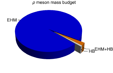
C	D

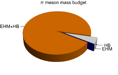
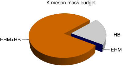
Figure 1: Mass budgets: A – proton; B – $\rho$-meson; C – pion; and D – kaon. Each is drawn using a Poincaré invariant decomposition and the numerical values listed in Table 1. (Separation at $\zeta=2\,GeV$, calculated using information from Refs. Flambaum et al. (2006); Ruiz de Elvira et al. (2018); Aoki et al. (2020); Workman et al. (2022).)

The information listed in rows 1, 2, 5, 6, of Table 1 is represented pictorially in Fig. 1: plainly, there are significant differences between the upper and lower panels. Regarding the proton and $\rho$-meson, the HB-alone component of their masses is just 1% in each case. Notwithstanding that, their masses are large, and remain so even in the absence of Higgs boson couplings into QCD, i.e., in the chiral limit. This overwhelmingly dominant component is a manifestation of EHM in the SM. It produces roughly 95% of the measured mass. Evidently, baryons and vector mesons are similar in these respects.

Conversely and yet still owing to EHM via its dynamical chiral symmetry breaking (DCSB) corollary, the pion is massless in the chiral limit – it is the SM’s Nambu-Goldstone (NG) mode Nambu (1960); Goldstone (1961); Gell-Mann et al. (1968); Casher and Susskind (1974); Brodsky and Shrock (2011); Brodsky et al. (2010); Chang et al. (2012); Brodsky et al. (2012); Cloet and Roberts (2014); Horn and Roberts (2016). Returning to the quark model picture, the only difference between $\rho$- and $\pi$-mesons is a spin-flip: in the $\rho$, the constituent quark spins are aligned, whereas they are antialigned in the $\pi$. Yet, their mass budgets are fundamentally different: Fig. 1B cf.  Fig. 1C. An inability to explain this difference is a conspicuous failure of quark models: whilst it is easy to obtain a satisfactory mass for the $\rho$, a low-mass pion can only be obtained by fine-tuning the quark model’s potential. Nature, however, doesn’t fine-tune the pion: in the absence of Higgs boson couplings, it is massless irrespective of the size of $m_{\rho}$ and, in fact, the mass of any other hadron.

The kaon mass budget is also drawn – see Fig. 1D. In the chiral limit, then, like the $\pi$, the $K$-meson is a NG boson. However, with realistic values of Higgs boson couplings into QCD, the $s$ quark current-mass is approximately $27$-times the average of the $u$ and $d$ current-masses Workman et al. (2022): $2m_{s}\approx 27(m_{u}+m_{d})$. Consequently, the HB wedge in Fig. 1D accounts for 20% of $m_{K}$. The remaining 80% is generated by constructive EHM+HB interference. It follows that comparisons between $\pi$ and $K$ properties present good opportunities for studying Higgs boson modulation of EHM, because the HB mass fraction is four-times larger in kaons than in pions. Moreover, the array of images in Fig. 1 highlight that additional, complementary information can be obtained from comparisons between baryons/vector-mesons and the array of kindred pseudoscalar mesons. For instance, studies of spectra (Sec. 6), transitions between vector-mesons and pseudoscalar mesons (Sec. 10), and comparative analyses of proton and pion parton distribution functions (DFs – see Sec. 11). In all cases, predominantly EHM systems on one hand are contrasted/overlapped with final states that possess varying degrees of EHM+HB interference.

These observations highlight that EHM – whatever it is – can be accessed via experiment. The task for theory is to identify and explain its source, then elucidate a broad range of observable consequences so that the origins and explanations can be validated.

3 Gluons and the Emergence of Mass

The requirement of gauge invariance ensures that the Higgs boson does not couple to gluons and precludes any other means of generating an explicit mass term for the gluon fields in Eq. (1). Consequently, it is widely believed that gluons are massless; and this is recorded by the Particle Data Group (PDG) (Workman et al., 2022, page 25). (We stress that gluon partons are massless.)

In QCD, this “gauge invariance” statement is properly translated into a property of the two-point gluon Schwinger function. Namely, using the class of covariant gauges as an illustrative tool, characterised by a gauge fixing parameter $\xi$, the inverse of the gluon two point function can be expressed in terms of a gluon vacuum polarisation (or self energy):

$$D_{\mu\nu}^{-1}(k)=\delta_{\mu\nu}k^{2}-k_{\mu}k_{\nu}(1-\xi)+\Pi_{\mu\nu}(k)=:\,_{0}D_{\mu\nu}^{-1}(k)+\Pi_{\mu\nu}(k)+\xi k_{\mu}k_{\nu}\,,$$ (2)

where $k$ is the gluon momentum. (Regarding $\xi$, common choices in perturbation theory are $\xi=0,1$, viz. Landau and Feynman gauges, respectively.) Gauge invariance (BRST symmetry of the quantised theory (Pascual and Tarrach, 1984, Ch. II)) is expressed in the following Slavnov-Taylor identity Taylor (1971); Slavnov (1972):

$$k_{\mu}\Pi_{\mu\nu}(k)=0=\Pi_{\mu\nu}(k)k_{\nu}\,.$$ (3)

This restrictive, yet generous, constraint states that interactions cannot affect the four-longitudinal component of the gluon two-point function, but leaves room for modifications of the propagation characteristics of the three four-transverse degrees-of-freedom.

Equation (3) means

$$\Pi_{\mu\nu}(k)=[\delta_{\mu\nu}k^{2}-k_{\mu}k_{\nu}]\Pi(k^{2})=:T_{\mu\nu}^{k}k^{2}\Pi(k^{2})\,,$$ (4)

where $\Pi(k^{2})$ is the dimensionless gluon self energy; hence, the gauge invariance constraint entails

$$D_{\mu\nu}(k)=T_{\mu\nu}^{k}\frac{1}{k^{2}[1+\Pi(k^{2})]}+\xi\frac{k_{\mu}k_{\nu}}{k^{4}}=:T_{\mu\nu}^{k}\overline{D}(k^{2})+\xi\frac{k_{\mu}k_{\nu}}{k^{4}}\,.$$ (5)

This is the propagator of a massless vector-boson unless

$$\Pi(k^{2})\stackrel{{\scriptstyle k^{2}\simeq 0}}{{=}}\frac{m_{J}^{2}}{k^{2}},$$ (6)

in the event of which both the dressed-gluon acquires a mass and all symmetry constraints are preserved. That Eq. (6) is possible in an interacting quantum gauge field theory was first shown in a study of two-dimensional QED Schwinger (1962a, b) and the phenomenon is now known as the Schwinger mechanism of gauge boson mass generation. Three-dimensional QED supports a similar outcome Appelquist et al. (1988); Maris (1996); Bashir et al. (2008, 2009); Braun et al. (2014), as does $D=3$ QCD Aguilar et al. (2010); Cornwall (2016); but, as already noted above, there is a difference between both these examples and QCD. Namely, whereas the Lagrangian couplings in $D<4$ theories carry a mass dimension, which explicitly breaks scale invariance, this is not the case for $D=4$ chromodynamics.

The existence of a Schwinger mechanism in QCD was first conjectured forty years ago Cornwall (1982). The idea has subsequently been explored and refined Aguilar et al. (2008); Boucaud et al. (2008); Binosi and Papavassiliou (2009); Boucaud et al. (2012); Aguilar et al. (2016), so that today a detailed picture is emerging, which unifies both the gauge and matter sectors Binosi et al. (2015). The dynamical origin of the QCD Schwinger mechanism and its intimate connection with nonperturbative dynamics in the three-gluon vertex are elucidated elsewhere Binosi (2022); Papavassiliou (2022). This is an area of continuing research, where synergies between continuum and lattice QCD are being exploited Aguilar et al. (2022); Pinto-Gómez et al. (2022). For our purposes, it is sufficient to know that Eq. (6) is realised in QCD. Indeed, owing to their self-interactions, gluon partons transmogrify into gluon quasiparticles whose propagation characteristics are determined by a momentum-dependent mass function. That mass function is power-law suppressed in the ultraviolet – hence, invisible in perturbation theory; yet large at infrared momenta, being characterised by a renormalisation point independent value Cui et al. (2020):

$$m_{0}=0.43(1)\,{\rm GeV}.$$ (7)

The renormalisation group invariant (RGI) gluon mass function is drawn in Fig. 2.

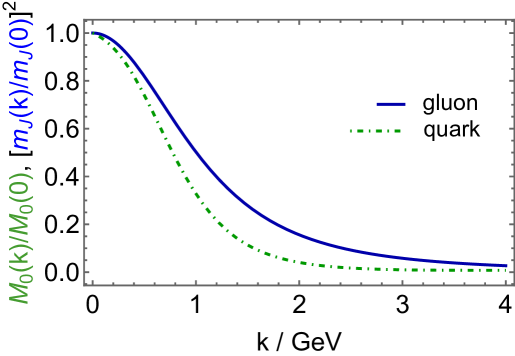
Figure 2: Renormalisation group invariant dressed-gluon mass function (solid blue curve) calculated, following the method in Ref. Aguilar et al. (2020), from a gluon two-point function obtained using the lQCD configurations in Refs. Blum et al. (2016); Boyle et al. (2016, 2017). The mass-squared curve is plotted, normalised by its $k=0$ value, and compared with the kindred chiral-limit dressed-quark mass function drawn from Ref. Binosi et al. (2017) (dot-dashed green curve). It is this pair of curves that is $1/k^{2}$-suppressed in the ultraviolet, each with additional logarithmic corrections.

Before closing this section, it is worth stressing the importance of Poincaré covariance in modern physics. If one chooses to formulate a problem in quantum field theory using a scheme that does not ensure Poincaré invariance of physical quantities, then artificial or “pseudodynamical” effects are typically encountered Brodsky et al. (2022). In connection with gauge theory Schwinger functions, Poincaré covariance very effectively limits the nature and number of independent amplitudes that are required for a complete representation. In contrast, analyses and quantisation procedures which violate Poincaré covariance engender a rapid proliferation in the number of such functions. For instance, the covariant-gauge gluon two-point function in Eq. (5) is fully specified by one scalar function; whereas in the class of axial gauges, two unconnected functions are required and unphysical, kinematic singularities appear in the associated tensors West (1983); Brown and Pennington (1989). This is why covariant gauges are normally employed for concrete calculations in both continuum and lattice-regularised QCD. In fact, Landau gauge, i.e., $\xi=0$ in Eq. (5), is often used because, amongst other things, it is a fixed point of the renormalisation group (Pascual and Tarrach, 1984, Ch. IV) and implemented readily in lQCD Cucchieri et al. (2009). We typically refer to Landau gauge results herein. Naturally, gauge covariance of Schwinger functions ensures that expressions of EHM in physical observables are independent of the gauge used for their elucidation.

Equation (7) is the cleanest expression of EHM in Nature, being truly a manifestation of mass emerging from nothing: infinitely many massless gluon partons fuse together so that, to all intents and purposes, they behave as coherent quasiparticle fields with a long-wavelength mass which is almost half that of the proton. The implications of this result are enormous and far-reaching, including, e.g., key steps toward elimination of the problem of Gribov ambiguities Gao et al. (2018), which were long thought to prevent a rigorous definition of QCD.

4 Process-Independent Effective Charge

In classical field theories, couplings and masses are constants. Typically, this is also true in quantum mechanics models of strong interaction phenomena. However, it is not the case in renormalisable quantum gauge field theories, as highlighted by the Gell-Mann–Low effective-charge/running-coupling in QED Gell-Mann and Low (1954), which is a textbook case (Itzykson and Zuber, 1980, Ch. 13.1).

A highlight of twentieth century physics was the realisation that QCD in particular, and non-Abelian gauge theories in general, express asymptotic freedom Politzer (2005); Wilczek (2005); Gross (2005), (Pickering, 1999, Ch. 7.1), i.e., the feature that the interaction between charge-carriers in the theory becomes weaker as $k^{2}$, the momentum-squared characterising the scattering process, becomes larger. Analysed perturbatively at one-loop order in the modified minimal subtraction renormalisation scheme, $\overline{MS}$, the QCD running coupling takes the form

$$\alpha_{\overline{MS}}(k^{2})=\frac{\gamma_{m}\pi}{\ln k^{2}/\Lambda_{\rm QCD}^{2}}\,,$$ (8)

where $\gamma_{m}=12/[33-2n_{f}]$, with $n_{f}$ the number of quark flavours whose mass does not exceed $k^{2}$, and $\Lambda_{\rm QCD}\sim 0.2\,$GeV is the RGI mass-parameter that sets the scale for perturbative analyses.

Asymptotic freedom comes with a “flip side”, which came to be known as infrared slavery (Marciano and Pagels, 1978, Sec. 3.1.2). Namely, beginning with some $k^{2}\gg\Lambda_{\rm QCD}^{2}$, then the interaction strength grows as $k^{2}$ is reduced, with the coupling diverging at $k^{2}=\Lambda_{\rm QCD}^{2}$. (This is the Landau pole.) Qualitatively, this statement is true at any finite order in perturbation theory: whilst the value of $\Lambda_{\rm QCD}$ changes somewhat, the divergence remains. In concert with the area law demonstrated in Ref. Wilson (1974), which entails that the potential between any two infinitely massive colour sources grows linearly with their separation, many practitioners were persuaded that the complex dynamical phenomenon of confinement could simply be explained by an unbounded potential that grows with parton separation. As we shall see, that is not the case, but the notion is persistent.

Given the character of QCD’s perturbative running coupling, two big questions arise:

1. does QCD possess a unique, nonperturbatively well-defined and calculable effective charge, viz. a veritable analogue of QED’s Gell-Mann–Low running coupling; and

2. does Eq. (8) express the large-$k^{2}$ behaviour of that charge?

If both questions can be answered in the affirmative, then great strides have been made toward verifying that QCD is truly a theory.

Following roughly forty years of two practically disjoint research efforts, one focused on QCD’s gauge sector Fischer (2006); Boucaud et al. (2012); Aguilar et al. (2016) and another on its matter sector Maris and Roberts (2003); Chang et al. (2011); Bashir et al. (2012); Roberts (2015), a key step on the path to answering these questions was taken in Ref. Binosi et al. (2015). The two distinct efforts were designated therein as the top-down approach – ab initio computation of the interaction via direct analyses of gauge-sector gap equations; and the bottom-up scheme – inferring the interaction by describing data within a well-defined truncation of those matter sector equations that are relevant to bound-state properties. Reference Binosi et al. (2015) showed that the top-down and bottom-up approaches are unified when the RGI running-interaction predicted by then-contemporary analyses of QCD’s gauge sector is used to explain ground-state hadron observables using nonperturbatively-improved truncations of the matter sector bound-state equations. The first such truncation was introduced in Ref. Chang and Roberts (2009).

It was a short walk from this point to a realisation Binosi et al. (2017) that in QCD, by means of the pinch-technique Pilaftsis (1997); Binosi and Papavassiliou (2009); Cornwall et al. (2010) and background field method Abbott (1982), one can define and calculate a unique, process-independent (PI) and RGI analogue of the Gell-Mann–Low effective charge, now denoted $\hat{\alpha}(k^{2})$. The analysis was refined in Ref. Cui et al. (2020), which combined modern results from continuum analyses of QCD’s gauge sector and lQCD configurations generated with three domain-wall fermions at the physical pion mass Blum et al. (2016); Boyle et al. (2016, 2017) to obtain a parameter-free prediction of $\hat{\alpha}(k^{2})$. The resulting charge is drawn in Fig. 3. It is reliably interpolated by writing

$$\hat{\alpha}(k^{2}) =\frac{\gamma_{m}\pi}{\ln\left[{\mathpzc K}^{2}(k^{2})/\Lambda_{\rm QCD}^{2}\right]}\,,\;{\mathpzc K}^{2}(y=k^{2})=\frac{a_{0}^{2}+a_{1}y+y^{2}}{b_{0}+y}\,,$$ (9)

with (in GeV²): $a_{0}=0.104(1)$, $a_{1}=0.0975$, $b_{0}=0.121(1)$. The curve was obtained using a momentum-subtraction renormalisation scheme: $\Lambda_{\rm QCD}=0.52\,$GeV when $n_{f}=4$.

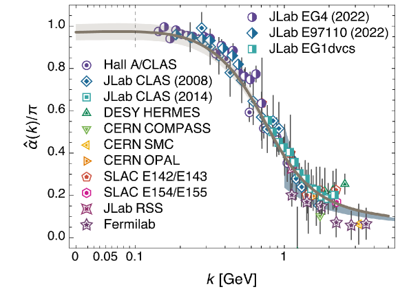
Figure 3: Process-independent effective charge, $\hat{\alpha}(k)/\pi$, obtained by combining modern results from continuum and lattice analyses of QCD’s gauge sector Cui et al. (2020). Existing data on the process-dependent charge $\alpha_{g_{1}}$ Deur et al. (2016, 2022), defined via the Bjorken sum rule, is shown for comparison – see Refs. Deur et al. (2007, 2008, 2014, 2022); Ackerstaff et al. (1997, 1998); Airapetian et al. (1998, 2003, 2007); Kim et al. (1998); Alexakhin et al. (2007); Alekseev et al. (2010); Adolph et al. (2016); Anthony et al. (1993); Abe et al. (1995a, b, 1996, 1995); Anthony et al. (1996); Abe et al. (1997a, b, c, 1998); Anthony et al. (1999a, b, 2000, 2003). (Image courtesy of D. Binosi.)

Notably, $\hat{\alpha}(k^{2})$ is PI and RGI in any gauge; but it is sufficient to know $\hat{\alpha}(k^{2})$ in Landau gauge, $\xi=0$ in Eq. (5), which is the choice both for easiest calculation and the result in Eq. (9). This is because $\hat{\alpha}(k^{2})$ is form invariant under gauge transformations, as may be shown using identities discussed elsewhere Binosi and Quadri (2013), and gauge covariance ensures that any such transformations can be absorbed into the Schwinger functions of the quasiparticles whose interactions are described by $\hat{\alpha}(k^{2})$ Aslam et al. (2016).

The following physical features of $\hat{\alpha}$ deserve to be highlighted because they expose a great deal about QCD.

Absence of a Landau pole.

Whereas the perturbative running coupling, e.g., Eq. (8), diverges at $k^{2}=\Lambda_{\rm QCD}^{2}$, revealing the Landau pole, the PI charge is a smooth function on $k^{2}\geq 0$: the Landau pole is eliminated owing to the appearance of a gluon mass scale, Eq. (7).

Implicit in the “screening function”, ${\mathpzc K}(k^{2})$, is a screening mass,

$$\zeta_{\cal H}={\mathpzc K}(k^{2}=\Lambda^{2}_{\rm QCD})\approx 1.4\,\Lambda_{\rm QCD}<m_{p},$$ (10)

at which point the perturbative coupling would diverge but the PI coupling passes through an inflection point on its way to saturation. On $\surd k^{2}\lesssim\zeta_{\cal H}$, the PI charge enters a new domain, upon which the running slows, practically ceasing on $\surd k^{2}\leq m_{0}/2$ so that QCD is once again effectively a conformal theory and the charge saturates to a constant infrared value $\hat{\alpha}(k^{2}=0)=\pi\times 0.97(4)$. This value is a prediction: within 3(4)%, the coupling saturates to a value of $\pi$ at $k^{2}=0$. It is not yet known whether this proximity to $\pi$ has any deeper significance in Nature, but a potential explanation is provided in the next bullet.

These features emphasise the role of EHM as expressed in Eq. (7): the existence of $m_{0}\approx m_{p}/2$ guarantees that long wavelength gluons are screened, so play no dynamical role. Consequently, $\zeta_{H}$ marks the boundary between soft/nonperturbative and hard/perturbative physics. It is therefore a natural choice for the “hadron scale”, viz. the renormalisation scale at which valence quasiparticle degrees-of-freedom should be used to formulate and solve hadron bound-state problems Cui et al. (2020). Implementing that notion, then those quasiparticles carry all hadron properties at $\zeta=\zeta_{\cal H}$. This approach is today being used to good effect in the prediction of hadron parton distribution functions (DFs) – see Sec. 11 and Refs. Ding et al. (2020a, b); Cui et al. (2021, 2020); Han et al. (2021); Chang and Roberts (2021); Xie et al. (2022); Raya et al. (2022); Cui et al. (2022a, b); Chang et al. (2022); Lu et al. (2022); de Paula et al. (2022).

Match with the Bjorken process-dependent charge.

The theory of process dependent (PD) charges was introduced in Ref. Grunberg (1984, 1989): “…to each physical quantity depending on a single scale variable is associated an effective charge, whose corresponding Stückelberg – Peterman – Gell-Mann–Low function is identified as the proper object on which perturbation theory applies." PD charges have since been widely canvassed Dokshitzer (1998); Prosperi et al. (2007); Deur et al. (2016).

One of the most fascinating things about the PI running coupling is highlighted by its comparison with the data in Fig. 3, which express measurements of the PD effective charge, $\alpha_{g_{1}}(k^{2})$, defined via the Bjorken sum rule Bjorken (1966, 1970). The charge calculated in Ref. Cui et al. (2020) is an essentially PI charge. There are no parameters; and, prima facie, no reason to expect that it should match $\alpha_{g_{1}}(k^{2})$. The almost precise agreement is a discovery, given more weight by new results on $\alpha_{g_{1}}(k^{2})$ Deur et al. (2022), which now reach into the conformal window at infrared momenta.

Mathematically, at least part of the explanation lies in the fact that the Bjorken sum rule is an isospin non-singlet relation, which eliminates many dynamical contributions that might distinguish between the two charges. It is known that the two charges are not identical; yet, equally, on any domain for which perturbation theory is valid, the charges are nevertheless very much alike:

$$\frac{\alpha_{g_{1}}(k^{2})}{\hat{\alpha}(k^{2})}\stackrel{{\scriptstyle k^{2}\gg m_{0}^{2}}}{{=}}1+\frac{1}{20}\alpha_{\overline{\rm MS}}(k^{2})\,,$$ (11)

where $\alpha_{\overline{\rm MS}}$ is given in Eq. (8). At the $c$ quark current-mass, the ratio is $1.007$, i.e., indistinguishable from unity insofar as currently achievable precision is concerned. At the other extreme, in the far infrared, the Bjorken charge saturates to $\alpha_{g_{1}}(k^{2}=0)=\pi$; hence,

$$\frac{\alpha_{g_{1}}(k^{2})}{\hat{\alpha}(k^{2})}\stackrel{{\scriptstyle k^{2}\ll m_{0}^{2}}}{{=}}1.03(4)\,.$$ (12)

Evidently, the PD charge determined from the Bjorken sum rule is, for practical intents and purposes, indistinguishable from the PI charge generated by QCD’s gauge-sector dynamics Binosi et al. (2017); Cui et al. (2020).

Infrared completion.

Being process independent, $\hat{\alpha}(k^{2})$ serves numerous purposes and unifies many observables. It is therefore a good candidate for that long-sought running coupling which describes QCD’s effective charge at all accessible momentum scales Dokshitzer (1998), from the deep infrared to the far ultraviolet, and at all scales in between, without any modification.

Significantly, the properties of $\hat{\alpha}(k^{2})$ support a conclusion that QCD is actually a theory, viz. a well-defined $D=4$ quantum gauge field theory. QCD therefore emerges as a viable tool for use in moving beyond the SM by giving substructure to particles that today seem elementary. A good example was suggested long ago; namely, perhaps all spin-$J=0$ bosons may be Schwinger (1962b) “…secondary dynamical manifestations of strongly coupled primary fermion fields and vector gauge fields …’. Adopting this position, the SM’s Higgs boson might also be composite; in which case, inter alia, the quadratic divergence of Higgs boson mass corrections would be eliminated.

Qualitatively equivalent remarks have been developed using light-front holographic models of QCD based on anti-de Sitter/conformal field theory (AdS/CFT) duality Brodsky and de Téramond (2004); Brodsky et al. (2010).

Returning to the two questions posed following Eq. (8) in items (a), (b), it is now apparent that they are answerable in the affirmative: QCD does possess a unique, nonperturbatively well-defined and calculable effective charge whose large-$k^{2}$ behaviour connects smoothly with that in Eq. (8). These facts provide strong support for the view that QCD is a well-defined 4D quantum gauge field theory.

5 Confinement

Confinement is much discussed but little understood. In large part, both these things stem from the absence of a clear, agreed definition of confinement. With certainty, it is only known that nothing with quantum numbers matching those of the gluon or quark fields in Eq. (1) has ever reached a detector.

An interpretation of confinement is included in the official description of the Yang-Mills Millennium Problem Carlson et al. (2006). The simpler background statement is worth repeating:
        “Quantum Yang-Mills theory is now the foundation of most of elementary particle theory, and its predictions have been tested at many experimental laboratories, but its mathematical foundation is still unclear. The successful use of Yang-Mills theory to describe the strong interactions of elementary particles depends on a subtle quantum mechanical property called the ‘mass gap’: the quantum particles have positive masses, even though the classical waves travel at the speed of light. This property has been discovered by physicists from experiment and confirmed by computer simulations, but it still has not been understood from a theoretical point of view. Progress in establishing the existence of the Yang-Mills theory and a mass gap will require the introduction of fundamental new ideas both in physics and in mathematics.”

The formulation of this problem focuses entirely on quenched-QCD, i.e., QCD without quarks; so, its solution is not directly relevant to our Universe. Confinement in pure quantum SU$(3)$ gauge theory and in QCD proper are probably very different because the pion exists and is unnaturally light on the hadron scale Horn and Roberts (2016). On the other hand, the remarks concerning the emergence of a “mass gap” relate directly to Fig. 2 and Eq. (7) herein. Whilst these properties of QCD may be considered proven by the canons of theoretical physics, such arguments do not meet the standards of mathematical physics and constructive field theory because they involve input from numerical analyses of QCD Schwinger functions. Hereafter, therefore, we will continue within the theoretical physics perspective.

As noted above, a mechanism for the total confinement of infinitely massive charge sources has been identified in the lattice-regularised treatment of quantum field theories using compact representations of Abelian or non-Abelian gauge fields Wilson (1974), viz. the area law $\equiv$ linear source-antisource potential. However, no treatment of the continuum meson bound-state problem has yet been able to demonstrate how such an area law emerges as the masses of the meson’s valence degrees-of-freedom grow to infinity.

In the era of infrared slavery, it was widely assumed that some sort of nonperturbatively improved one-gluon exchange could simultaneously produce asymptotic freedom and a linearly rising potential between quarks; and many models were developed with just such features Eichten et al. (1978); Richardson (1979); Buchmuller and Tye (1981); Godfrey and Isgur (1985); Lucha et al. (1991). However, as highlighted by our discussion of QCD’s effective charge, ongoing developments in the study of mesons, using rigorous treatments of the Schwinger functions involved, do not support this picture of confinement via dressed-one-gluon-exchange. The path to an area law is far more complex.

A		B

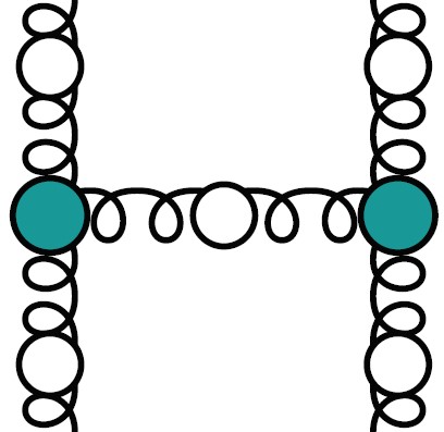
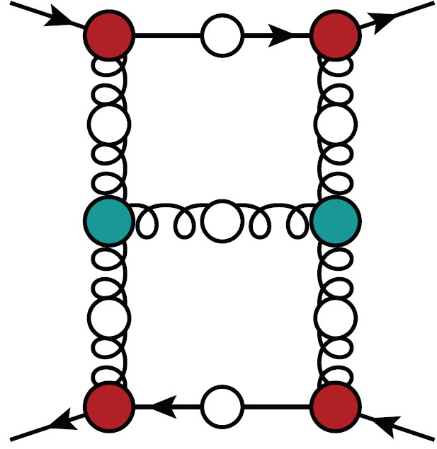
Figure 4: Panel A – primitive gluon $H$-diagram. Panel B – one-$H$-diagram contribution to quark+antiquark scattering. Legend. Dressed-gluon two-point function – spring with open circle insertion; dressed-quark two-point function – straight line with open circle insertion; blue-filled circle at $3$-gluon junction – dressed $3$-gluon vertex; and red-filled circle at gluon-quark junction – dressed gluon-quark. Repeated insertion of $H$-diagrams within $H$-diagrams, exploiting both gluon-quark and gluon self-couplings, leads to a plaquette-like area-filling structure, reminiscent of the planar summation of elementary squares in Ref. Wilson (1974).

One direction that deserves exploration is connected with the gluon “$H$-diagrams” drawn in Ref. (Binosi et al., 2016, Fig. 8) and reproduced in Fig. 4A. Imagine a valence-quark and -antiquark scattering via such a process, as drawn in Fig. 4B; then keep adding $H$-diagrams within $H$-diagrams, exploiting both gluon-quark and gluon self-couplings. Such $H$-diagram scattering processes produce an infrared divergence in the perturbative computation of a static quark potential Smirnov et al. (2010), viz. a contribution that exhibits unbounded growth as the source-antisource separation increases. Nonperturbatively, that divergence is tamed because the effective charge saturates – Fig. 3. On the other hand, there are infinitely many such contributions; and in the limit of static valence degrees-of-freedom, the entire unbounded sum of planar $H$-diagrams is contracted to a point-connection of infinitely dense fisherman’s-net/spider’s-web diagrams on both the source and antisource. It is conceivable that the confluence of these effects could yield the long-sought area law via the Bethe-Salpeter equation Binosi et al. (2016); Brodsky et al. (2015a).

Real-world QCD, however, is characterised by light degrees-of-freedom: $u$ and $d$ quarks with electron-size current masses; and $s$ quarks with mass roughly one order-of-magnitude larger, so still much less than $m_{p}$. Pions and kaons are constituted from such valence degrees-of-freedom and these mesons are light. In fact, the pion has a lepton like mass Workman et al. (2022): $m_{\pi}\approx m_{\mu}$, where $m_{\mu}$ is the mass of the $\mu$ lepton. Owing to the presence of such degrees-of-freedom, light-particle annihilation and creation effects are essentially nonperturbative in QCD. Consequently, despite continuing dedicated efforts Brodsky et al. (2015b); Reinhardt et al. (2018); Hoyer (2021), it has thus far proved impossible to either define or calculate a static quantum mechanical potential between two light quarks.

This may be illustrated by apprehending that a potential which increases with separation can be described by a flux tube extending between the source and antisource. As the source-antisource separation increases, so does the potential energy stored in the flux tube. However, it can only increase until the stored energy matches that required to produce a particle+antiparticle pair of the theory’s lightest asymptotic states – in QCD, a $\pi^{+}\pi^{-}$ pair. Numerical simulations of lQCD reveal Bali et al. (2005); Prkacin et al. (2006) that once the energy exceeds this critical value, the flux tube then dissolves along its entire length, leaving two isolated colour-singlet systems. Given that $m_{\pi}=0.14\,$GeV, then this disintegration must occur at source+antisource centre-of-mass separation $r\approx(1/3)\,$fm Chang et al. (2009), which is well within the interior of any hadron. This example assumes that the source and antisource are static. The situation is even more complex for real, dynamical quarks. Thus, at least in the $u$, $d$, $s$ quark sector, confinement is manifested in features of Schwinger functions that are far more subtle than can be captured in typical potential models.

One non-static, i.e., dynamical, picture of confinement has emerged from studies of the analytic properties of the two-point Schwinger functions associated with propagation of coloured gluon and quark quasiparticles – see, e.g., Fig. 2. The development of this perspective may be traced back to a beginning almost forty years ago Munczek and Nemirovsky (1983); Stingl (1986); Zwanziger (1989); Roberts et al. (1992); Burden et al. (1992); Gribov (1999). It has subsequently been carefully explored Burden et al. (1992); Stingl (1996); Roberts (2008); Dudal et al. (2008); Brodsky et al. (2012); Qin and Rischke (2013); Lucha and Schöberl (2016); Gao et al. (2018); Binosi and Tripolt (2020); Dudal et al. (2020); Fischer and Huber (2020); Roberts (2020); and in this connection one may profitably observe that only Schwinger functions which satisfy the axiom of reflection positivity Osterwalder and Schrader (1973, 1975); Glimm and Jaffee (1981) can be connected with states that appear in the Hilbert space of observables.

The axioms referred to here are those first presented in Refs. Osterwalder and Schrader (1973, 1975) and subsequently modified in Glimm and Jaffee (1981), which identify the properties of Schwinger functions that are necessary and sufficient to ensure equivalence between the formulation of a given quantum field theory in Euclidean and Minkowski space. (A contemporary literature compilation is presented elsewhere Dedushenko (2022).) In effect, this means that all and only those Schwinger functions which satisfy the five Osterwalder-Schrader axioms possess connections with elements in the Hilbert space of physical states. Regarding strong interactions, all physical states are colour singlets. Consequently, for QCD to be the theory of strong interactions, all its colour-singlet Schwinger functions must satisfy the Osterwalder-Schrader axioms; equally, all its colour-nonsinglet functions must violate at least one.

Reflection positivity is a severe constraint. It requires that the Fourier transform of the momentum-space Schwinger function, treated as a function of analytic, Poincaré-invariant arguments, is a positive-definite function. To illustrate, consider the gluon Schwinger function in Eq. (5). A massless partonic gluon is described by $\overline{D}(k^{2})=1/k^{2}$; and the $4D$ Fourier transform of this function is

$$\int\frac{d^{4}k}{(2\pi)^{4}}{\rm e}^{ik\cdot x}\frac{1}{k^{2}}=\frac{1}{4\pi^{2}x^{2}}>0\;\forall x^{2}>0\,.$$ (13)

More generally regarding two-point functions, viz. those connected with propagation of elementary excitations in QCD, reflection positivity is satisfied if, and only if, the Schwinger function has a Källén-Lehmann representation. Returning to the gluon Schwinger function in Eq. (5), this means one must be able to write

$$\overline{D}(k^{2})=\int_{0}^{\infty}d\zeta\frac{\rho(\varsigma)}{k^{2}+\varsigma^{2}}\,,\quad\rho(\varsigma)>0\;\forall\varsigma>0.$$ (14)

Plainly, $\rho(\varsigma)=\delta(\varsigma)$ yields $\overline{D}(k^{2})=1/k^{2}$, i.e., the two-point function for a bare gluon parton. Hence, according to Eqs. (13), (14), absent dressing, the gluon parton could appear in the Hilbert space of physical states.

It is important to observe that any function which satisfies Eq. (14) is positive definite itself. Moreover, given Eq. (14),

$$sgn\left([\frac{d}{dk^{2}}]^{n}\,\overline{D}(k^{2})\right)=(-1)^{n}\,;$$ (15)

consequently, inter alia, treated as a function of the analytic, Poincaré-invariant variable $k^{2}$, no function with a Källén-Lehmann representation of the form written in Eq. (14) can possess an inflection point. Conversely, any function that exhibits an inflection point or, more generally, has a second derivative which changes sign, must violate the axiom of reflection positivity Roberts (2008); hence, the associated excitation cannot appear in the Hilbert space of observables.

Take another step, and consider the following configuration space Schwinger function ($\tau=x_{4}$, $\ell=k_{4}$)

$$\Delta(\tau)=\int d^{3}x\int\frac{d^{4}k}{(2\pi)^{4}}{\rm e}^{ik\cdot x}\overline{D}(k^{2})=\frac{1}{\pi}\int_{0}^{\infty}d\ell\cos(\ell\tau)\overline{D}(\ell^{2})\,.$$ (16)

Suppose that interactions generate a constant mass for the gluon parton, so that $\overline{D}(k^{2})=1/(k^{2}+\mu^{2})$. Does that trigger confinement? The answer is "no" because this Schwinger function has a spectral representation with $\rho(\varsigma)=\delta(\varsigma^{2}-\mu^{2})$; Eq. (15) is satisfied; and so is positivity:

$$\Delta(\tau)=\frac{1}{2\mu}{\rm e}^{-\mu\tau}\,.$$ (17)

Suppose instead that interactions produce a momentum-dependent mass-squared function like that in Fig. 2, which is $1/k^{2}$ suppressed in the ultraviolet:

$$m_{J}^{2}(k^{2})=\frac{\mu_{0}^{4}}{k^{2}+\mu_{0}^{2}}\Rightarrow\overline{D}(k^{2})=\frac{k^{2}+\mu_{0}^{2}}{k^{2}(k^{2}+\mu_{0}^{2})+\mu_{0}^{4}}\,.$$ (18)

The mass function itself is a monotonically decreasing, concave-up function; yet, in this case, the Schwinger function has an inflection point at $k^{2}=0.53\mu_{0}^{2}$. Hence, it does not have a Källén-Lehmann representation; so, the associated excitation cannot appear in the Hilbert space of observables. Furthermore, evaluation of the configuration space Schwinger function defined by Eq. (16) yields Gao et al. (2018)

$$\Delta(\tau)=\frac{1}{\mu_{0}}{\rm e}^{-\tau\mu_{0}\tfrac{\surd 3}{2}}\cos\frac{\mu_{0}\tau}{2}=:\Delta_{\rm p}(\tau)\cos\frac{\mu_{0}\tau}{2}\,,$$ (19)

using which the curve in Fig. 5 is drawn: plainly, the configuration space Schwinger function violates reflection positivity. (Notably, the algebraic calculation of $\Delta(\tau)$ is often difficult and not always possible; so, uniform positivity of the second-derivative, Eq. (15), is a much quicker means of testing for reflection positivity. Nevertheless, when it can be obtained, an explicit form of $\Delta(\tau)$ does provide additional insights.)

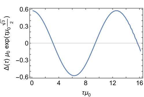
Figure 5: $\Delta(\tau)\mu_{0}\exp(\mu_{0}\tau\tfrac{\surd 3}{2})$ computed from the Schwinger function in Eq. (18) using Eq. (16).

It is interesting to extend Eq. (18) using $m_{J}^{2}(k^{2})=\alpha\mu_{0}^{4}/[k^{2}+\mu_{0}^{2}]$, in which case

$$\overline{D}(k^{2}=\mu_{0}^{2}y)=\frac{1}{\mu_{0}^{2}}\frac{1+y}{y^{2}+y+\alpha}=:\frac{1}{\mu_{0}^{2}}{\mathpzc d}(y)\,.$$ (20)

This type of Schwinger function lies within the so-called “refined Gribov-Zwanziger” class Dudal et al. (2008). For $\alpha>\tfrac{1}{2}$, as in the example above, the function in Eq. (20) exhibits an inflection point at some $y>0$; and when $\alpha\in(\tfrac{1}{4},\tfrac{1}{2})$, the inflection point is found at a location $y\in(-\tfrac{1}{2},0)$. With $\alpha\in(0,\tfrac{1}{4})$, on the other hand, the function in Eq. (20) separates into a sum of two terms:

$${\mathpzc d}(y)=\frac{\mathpzc n_{1}}{y+{\mathpzc p}_{1}}-\frac{\mathpzc n_{2}}{y+{\mathpzc p}_{2}}\,,$$ (21)

where ${\mathpzc p}_{1,2}\in\mathbb{R}$ and $sgn({\mathpzc p}_{1}/{\mathpzc p}_{2})=+1$. In this case, there is no inflection point; nevertheless, the second derivative does change sign, switching $\pm\infty\leftrightarrow\mp\infty$ as $y$ passes through the pole locations. Consequently, any excitation whose propagation is described by a Schwinger function obtained with $\alpha>0$ in Eq. (20) cannot appear in the Hilbert space of observable states.

Inserting Eq. (20) into Eq. (16), one finds, after some careful algebra Gao et al. (2018) (${\mathpzc a}=\alpha^{1/4}$):

$$\Delta(\tau) =\frac{1}{2\mu_{0}{\mathpzc a}s_{\varphi/2}}{\rm e}^{-\tau\mu_{0}{\mathpzc a}c_{\varphi/2}}$$

$$\quad\times\left[(1+\tfrac{1}{{\mathpzc a}^{2}})s_{\varphi/2}\cos(\tau\mu_{0}{\mathpzc a}s_{\varphi/2})-(1-\tfrac{1}{{\mathpzc a}^{2}})c_{\varphi/2}\sin(\tau\mu_{0}{\mathpzc a}s_{\varphi/2})\right]\,,$$ (22)

where $c_{\varphi/2}=[\tfrac{1}{2}+\tfrac{1}{4{\mathpzc a}^{2}}]^{1/2}$, $s_{\varphi/2}=[1-c_{\varphi/2}^{2}]^{1/2}$. (Eq. (19) is a special case of this result.) Equation (22) reveals that the distance from $\tau=0$ of the first zero in the configuration space Schwinger function, $\tau_{z}$, increases with decreasing $\alpha$, i.e., as the infrared value of the gluon mass-squared function is reduced. Thus, confinement would practically be lost if $\tau_{z}$ were to become much greater than $\pi/\mu_{0}$. Considering realistic gluon two-point functions, however, one finds $\mu_{0}\approx(3/4)m_{p}$, $\alpha\approx 1$ Gao et al. (2018); so, $\tau_{z}\approx 1\,$fm, expressing a natural confinement length-scale. (It is worth observing that if $\tau_{z}$ were instead measured on the Å scale, then the notion of confinement would be lost because modern detectors are able to directly image targets of this size Stodolna et al. (2013).)

This discussion is readily summarised. Owing to complex nonlinear dynamics in QCD, gluon and quark partons acquire momentum-dependent mass functions, as a consequence of which they emerge as quasiparticles whose propagation characteristics are described by two-point Schwinger functions that are incompatible with reflection positivity. Normally, the dynamical generation of running masses is alone sufficient to ensure this outcome. It follows that the dressed-gluons and -quarks cannot appear in the Hilbert space of physical states. In this sense, they are confined. The associated confinement length-scale is $\tau_{z}\approx 1\,$fm. It is worth stressing that the use of such two-point functions in the calculation of colour-singlet matrix elements ensures the absence of coloured particle+antiparticle production thresholds Bhagwat et al. (2003), thereby securing the empirical expression of real-QCD confinement.

Considering these quasiparticle Schwinger functions further, one may also define a parton persistence or fragmentation length, $\tau_{\rm F}$, as the scale whereat the deviation of the Schwinger function from parton-like behaviour is $50$%: $\Delta(\tau_{\rm F})/\Delta_{\rm p}(\tau_{\rm F})=0.5$. Referring to Eq. (19), one reads $\tau_{\rm F}=(2/3)\tau_{z}$. This result is also found using realistic gluon two-point functions Gao et al. (2018). (The value 50% is merely a reasonable choice. At this level, 30% would also be acceptable, in which case $\tau_{\rm F}\to\tau_{\rm F}^{\prime}=(1/2)\tau_{z}$.)

A physical picture of dynamical confinement now becomes apparent Stingl (1996). Namely, once a gluon or quark parton is produced, it begins to propagate in spacetime; but after traversing a spacetime distance characterised by $\tau_{\rm F}$, interactions occur, causing the parton to lose its identity, sharing it with others. Ultimately, combining the effects on this parton with similar impacts on those produced along with it, a countable infinity of partons (a parton cloud) is produced, from which detectable colour-singlet final states coalesce. This train of events is the physics expressed in parton fragmentation functions (FFs) Field and Feynman (1978). Such distributions describe how the QCD partons in Eq. (1), generated in a high-energy event and almost massless in perturbation theory, transform into a shower of massive hadrons, viz. they describe how hadrons with mass emerge from practically massless partons. It is natural, therefore, to view FFs as the cleanest expression of dynamical confinement in QCD. Furthermore, in the neighbourhood of their common boundary of support, DFs and FFs are related by crossing symmetry Gribov and Lipatov (1971): FFs are timelike analogues of DFs. Hence, an understanding of FFs and their deep connection with DFs can deliver fundamental insights into EHM. This picture of parton propagation, hadronisation and confinement – of DFs and FFs – can be tested in experiments at modern and planned facilities Brodsky et al. (2015); Denisov et al. (2018); Aguilar et al. (2019); Brodsky et al. (2020); Chen et al. (2020); Anderle et al. (2021); Arrington et al. (2021); Aoki et al. (2021); Quintans (2022). A pressing demand on theory is delivery of predictions for FFs before such experiments are completed so as, for instance, to guide development of facilities and detectors. As yet, however, there are no realistic computations of FFs. In fact, even a formulation of this problem remains uncertain.

Before moving on, it is worth reiterating that confinement means different things to different people. Whilst some see confinement only in an area law for Wilson loops Wilson (1974), our perspective stresses a dynamical picture, in which dynamically driven changes in the analytic structure of coloured Schwinger functions ensures the absence of colour-carrying objects from the Hilbert space of observable states. In time, perhaps, as strong QCD is better understood, it may be found that these two realisations are connected? The only certain thing is the necessity to keep an open mind on this subject.

6 Spectroscopy

Insofar as the spectrum of hadrons is concerned, results from nonrelativistic or somewhat relativised quark models Capstick and Roberts (2000); Giannini and Santopinto (2015); Plessas (2015) are still often cited as benchmarks. Indeed, a standard reference (Workman et al., 2022, Sec. 63) includes the following assertions: “The spectrum of baryons and mesons exhibits a high degree of regularity. The organizational principle which best categorizes this regularity is encoded in the quark model. All descriptions of strongly interacting states use the language of the quark model.” This is despite the fact that neither the “quarks” nor the potentials in quark models have been shown to possess any mathematical link with Eq. (1) – rigorous or otherwise; and, furthermore, the orbital angular momentum and spin used to label quark model states are not Poincaré-invariant (observable) quantum numbers.

In step with improvements in computer performance, lQCD is delivering interesting results for hadron spectra Dudek et al. (2010); Edwards et al. (2011), amongst which one may highlight indications for the existence of hybrid and exotic hadrons Liu et al. (2012); Dudek and Edwards (2012); Ryan and Wilson (2021); Woss et al. (2021). Continuum studies in quantum field theory are lagging behind owing in part to impediments placed by the character of the Bethe-Salpeter equation; primarily the fact that it is impossible to write the complete Bethe-Salpeter kernel in a closed form.

A systematic approach to truncating the integral equations associated with bound-state problems in QCD was introduced almost thirty years ago Munczek (1995); Bender et al. (1996). Amongst other things, the scheme highlighted the importance of preserving continuous and discrete symmetries when formulating bound-state problems; enabled proof of Goldberger-Treiman identities and the Gell-Mann–Oakes–Renner relation in QCD Maris et al. (1998); Maris and Roberts (1997); and opened the door to symmetry-preserving, Poincaré-invariant predictions of hadron observables, including elastic and transition form factors and DFs Maris and Roberts (2003); Chang et al. (2011); Bashir et al. (2012); Roberts (2015); Eichmann et al. (2016); Chen et al. (2018); Ding et al. (2019); Eichmann et al. (2020); Xu et al. (2019, 2021); Yao et al. (2020, 2021, 2022); Ding et al. (2020b). Some of the more recent developments are sketched below.

An issue connected with the leading-order (RL - rainbow-ladder) term in the truncation scheme of Refs. Munczek (1995); Bender et al. (1996) is that it only serves well for those ground-state hadrons which possess little rest-frame orbital angular momentum, $L$, between the dressed valence constituents Höll et al. (2004, 2005); Fischer and Williams (2009); Krassnigg (2009); Qin et al. (2011, 2012); Blank and Krassnigg (2011); Hilger et al. (2015); Fischer et al. (2015); Eichmann et al. (2016); Qin et al. (2019). This limitation can be traced to its inability to realistically express impacts of EHM on hadron observables, a weakness that is not overcome at any finite order of elaboration Fischer and Williams (2009). Improved schemes, which express EHM in the kernels, have been identified Chang and Roberts (2009, 2012); Binosi et al. (2015); Williams et al. (2016); Binosi et al. (2016); Qin and Roberts (2021). They have shown promise in applications to ground-state mesons constituted from $u$, $d$ valence quarks and/or antiquarks. However, that is a small subset of the hadron spectrum; so, a recent extension to the spectrum and decay constants of $u$, $d$, $s$ meson ground- and first-excited states is welcome Xu et al. (2022).

Returning to quark models, it was long ago claimed Godfrey and Isgur (1985) “…that all mesons – from the pion to the upsilon – can be described in a unified framework.” The context for this assertion was a model potential built using one-gluon-like exchange combined with an infrared-slavery “confinement” term that increases linearly with colour-source separation. The basic mass-scales in such potential models are set by the constituent quark masses; and one might draw a qualitative link between those scales and the far-infrared values of the momentum-dependent dressed-quark running-masses (Roberts et al., 2021, Fig. 2.5): $M_{u,d}(0)\simeq 0.41\,$GeV, $M_{s}(0)\simeq 0.53\,$GeV. Thereafter, mass-splittings and level orderings are arranged by tuning details of the potential. Such a procedure can be quantitatively efficacious; however, it is qualitatively incorrect. This is readily seen by recalling the Gell-Mann–Oakes–Renner relation Gell-Mann et al. (1968); Maris et al. (1998); Qin et al. (2014): $m_{\pi}^{2}\propto\hat{m}$, where $\hat{m}$ is Nature’s explicit source of chiral symmetry breaking, generated by Higgs boson couplings to quarks in the SM. Such behaviour is impossible in a potential model Roberts (2015); Horn and Roberts (2016), but natural in the CSM treatment of bound-states – see, e.g., Refs. Maris et al. (1998); Höll et al. (2004), (Maris and Roberts, 2003, Fig. 3.3), (Bhagwat et al., 2004, Fig. 7), (Chang and Roberts, 2009, Fig. 1A). Thus, whilst potential models might deliver a fit to hadron spectra, they do not provide an explanation.

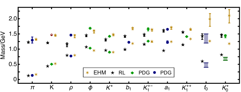
Figure 6: Empirical spectrum (Workman et al., 2022, PDG Summary Tables): blue circles (bars) – $u$, $d$ states; and green diamonds (bar) – systems with $s$ and/or $\bar{s}$ quarks. Little is known about $K(1460)$, which is therefore drawn as an open red diamond. Gold six-pointed stars – spectrum of low-lying $u$, $d$, $s$ mesons predicted by the EHM-improved Bethe-Salpeter kernel developed in Ref. Xu et al. (2022); and black five-pointed stars – same spectrum computed using RL truncation.

That such challenges are surmounted when using CSMs to treat hadron bound-state problems is further exemplified in Ref. Xu et al. (2022), which adapts a novel scheme for including EHM effects in the Bethe-Salpeter kernel Qin and Roberts (2021) to simultaneously treat ground- and first-excited-states of $u$, $d$, $s$ quarks. As revealed in Fig. 6, the empirical spectrum displays some curious features, e.g.: consistent with quark mass-scale counting, $m_{\rho}<m_{K^{\ast}}$, but this ordering is reversed for the first excitations of these states; the first excited state of the $\pi$ is lighter than that of the $\rho$, but the ordering is switched for $K$, $K^{\ast}$; and all axialvector mesons are nearly degenerate, with the larger mass of the $s$ quarks appearing to have little or no impact. In delivering the first symmetry-preserving analysis of this collection of states to employ an EHM-improved kernel, Ref. Xu et al. (2022) supplies fresh insights into the dynamical foundations of the properties of lighter-quark mesons.

In order to sketch that effort, we note that, using CSMs, the dressed propagator (two-point Schwinger function) for a quark with flavour $g$ is obtained as the solution of the following gap equation:

$$S_{g}^{-1}(k) =i\gamma\cdot k\,A_{g}(k^{2})+B_{g}(k^{2})=[i\gamma\cdot k+M_{g}(k^{2})]/Z_{g}(k^{2})\,,$$ (23a)

$$=Z_{2}\,(i\gamma\cdot k+m_{g})+\Sigma_{g}(k)\,,$$ (23b)

$$\Sigma(k) =Z_{1}\int^{\Lambda}_{dq}\!\!g^{2}D_{\mu\nu}(k-q)\frac{\lambda^{a}}{2}\gamma_{\mu}S_{g}(q)\frac{\lambda^{a}}{2}\Gamma_{\nu}^{g}(k,p),$$ (23c)

where $M_{g}(k^{2})$ is RGI;

$$D_{\mu\nu}(k)=\Delta(k^{2})\,_{0}D_{\mu\nu}(k)\,;$$ (24)

$\Gamma_{\nu}^{g}$ is the quark-gluon vertex; $\int^{\Lambda}_{dq}$ denotes a Poincaré invariant regularisation of the four-dimensional integral, with $\Lambda$ the regularisation mass-scale; and $Z_{1,2}(\zeta^{2},\Lambda^{2})$ are, respectively, the vertex and quark wave-function renormalisation constants, with $\zeta$ the renormalisation point. (In such applications, when renormalisation is necessary, a mass-independent scheme is important, as discussed elsewhere Chang et al. (2009).)

It was anticipated almost forty years ago Singh (1985); Bicudo et al. (1999), and confirmed more recently Chang et al. (2011); Bashir et al. (2012); Binosi et al. (2017); Kızılersü et al. (2021), that EHM engenders a large anomalous chromomagnetic moment (ACM) for the lighter quarks; and with development of the first EHM-improved kernels, it was shown that such an ACM has a big impact on the $u$, $d$ meson spectrum Chang and Roberts (2012); Williams et al. (2016); Qin and Roberts (2021).

The aim in Ref. Xu et al. (2022) was to extend Refs. Chang and Roberts (2012); Williams et al. (2016); Qin and Roberts (2021) and highlight additional impacts of an ACM on the spectrum of mesons constituted from $u$, $d$, $s$ quarks. An ACM emerges as a feature of the dressed-gluon-quark vertex, a three-point Schwinger function. Its character and impacts can be exposed by writing $(l=k-q)$

$$\Gamma_{\nu}^{g}(q,k)=\gamma_{\nu}+\tau_{\nu}(l)\,,\;\tau_{\nu}(l)=\eta\kappa(l^{2})\sigma_{l\nu}\,,$$ (25)

$\sigma_{l\nu}=\sigma_{\rho\nu}l_{\rho}$, $\kappa(l^{2})=(1/\omega)\exp{(-l^{2}/\omega^{2})}$. Here, $\eta>0$ is the strength of the ACM term, $\tau_{\nu}(l)$; and it is assumed that the vertex is flavour-independent, which is a sound approximation for the lighter quarks Bhagwat et al. (2004); Williams (2015). When considering Eq. (25), one might remark that the complete gluon-quark vertex is far more complicated – potentially containing twelve distinct terms – and, in QCD, $\kappa(l^{2})$ is power-law suppressed in the ultraviolet. Notwithstanding these things, illustrative purposes are well served by Eq. (25).

ACM effects are most immediately felt by the dressed-quark propagator. The presence of an ACM in the kernel of Eq. (23) increases positive EHM-induced feedback on dynamical mass generation. Consequently, as shown elsewhere Binosi et al. (2017), realistic values of the dressed-quark mass at infrared momenta are achieved using the PI effective charge in Fig. 3. Such an outcome requires tuning when using the PI charge in a rainbow truncation of the gap equation; in fact, DCSB cannot be guaranteed in that case Binosi et al. (2015).

Following Refs. Chang and Roberts (2009); Chang et al. (2011); Qin and Roberts (2021) in continuing to emphasise clarity over numerical complexity, Ref. Xu et al. (2022) also simplified the kernel in Eq. (23), writing

$$g^{2}\Delta(k^{2})=4\pi\hat{\alpha}(0)\frac{D(\eta)}{\omega^{4}}{\rm e}^{-k^{2}/\omega^{2}}\,,$$ (26)

where $\omega=0.8\,$GeV, a value matching that suggested by analyses of QCD’s gauge sector Binosi et al. (2015); Cui et al. (2020), and $D(\eta)=D_{\rm RL}(1+0.27\eta)/(1+1.47\eta)$, with $\omega D_{\rm RL}=(1.286\,{\rm GeV})^{3}$ chosen to achieve $m_{\rho}=0.77\,$GeV in RL truncation. The $\eta$-dependence of $D(\eta)$ was fixed a posteriori by requiring that $m_{\rho}$ remain unchanged as $\eta$ is increased. Since $\eta>0$ adds EHM strength to the gap equation’s kernel, then $D$ must become smaller as $\eta$ grows in order to maintain a fixed value of $m_{\rho}$. Following this procedure, $m_{\rho}$ becomes the benchmark against which all ACM-induced changes are measured.

It is worth noting that when one identifies $(g^{2}/[4\pi])\Delta(k^{2}=0)=1/\mu_{0}^{2}$, then $\mu_{0}=0.39\,$GeV in RL truncation and $\mu_{0}=0.57\,$GeV at $\eta=1.2$. So, the interaction specified by Eq. (26) is consistent with gluon mass generation as described in Sec. 3. On the other hand, the large-$k^{2}$ behaviour of Eq. (26) does not respect the renormalisation group flow of QCD. This would be an issue if one were using it, e.g., to calculate hadron form factors at large $Q^{2}$ Chen et al. (2018); Ding et al. (2019); Xu et al. (2019, 2021), where $Q^{2}$ is momentum transfer squared, or parton distribution functions and amplitudes near the endpoints of their support domains Ding et al. (2020a, b); Cui et al. (2021, 2020). However, it is far less important when calculating global, integrated properties, like hadron masses. In such applications, Eq. (26) is satisfactory. Indeed, good results can even be obtained using a symmetry-preserving treatment of a momentum-independent interaction Yin et al. (2021); Xu et al. (2021); Gutiérrez-Guerrero et al. (2021). A key merit of Eq. (26) lies in its elimination of the need for renormalisation, which simplifies analyses without materially affecting relevant results.

The scheme introduced in Ref. Qin and Roberts (2021) provides a direct route from any reasonable set of gap equation elements to closed-form Bethe-Salpeter kernels for meson bound-state problems. Thus having specified physically reasonable gap equations via Eqs. (25), (26), Ref. Xu et al. (2022) adapted that scheme to arrive at Bethe-Salpeter equations for each of the mesons identified in Fig. 6, obtaining solutions in all cases. The image compares experiment with RL truncation results, also calculated in Ref. Xu et al. (2022), and predictions obtained using the EHM-improved kernel.

It is first worth mentioning the RL truncation mass predictions in Fig. 6. On the whole, the mean absolute relative difference, $\overline{\mbox{ard}}$, between RL results and central experimental values is $13(8)$%. This is tolerable; but there is substantial scatter and there are many qualitative discrepancies.

In contrast, compared with central experimental values, the EHM-improved masses in Fig. 6 agree at the level of $\overline{\mbox{ard}}=2.9(2.7)$%. This is a factor of $4.6$ improvement over the RL spectrum. Moreover, correcting RL truncation flaws and reproducing empirical results: $m_{K^{\prime}}>m_{\pi^{\prime}}$, $m_{\rho^{\prime}}>m_{\pi^{\prime}}$, $m_{\rho^{\prime}}\approx m_{K^{\ast\prime}}$; the mass splittings $a_{1}$-$\rho$ and $b_{1}$-$\rho$ match empirical values because including the ACM in the kernel has markedly increased the masses of the $a_{1}$ and $b_{1}$ mesons, whilst $m_{\rho}$ was deliberately kept unchanged; $m_{\phi^{\prime}}-m_{\phi}$ agrees with experiment to within 2%; the $K_{1}^{+-}$, $K_{1}^{++}$ level order is correct; and quark+antiquark scalar mesons are heavy, providing room for the addition of strongly attractive resonant contributions to the bound-state kernels Höll et al. (2006); Santowsky et al. (2020).

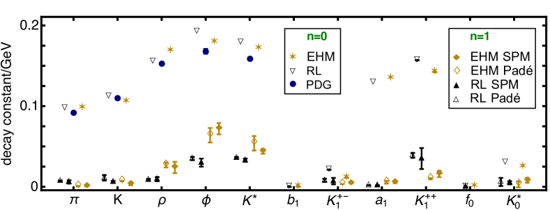
Figure 7: Leptonic decay constants for all states whose masses are reported in Fig. 6: ground states, $n=0$; and lowest lying radial excitations, $n=1$. For the excited states, two extrapolation results are presented for each state, viz. one obtained with Padé approximants and the other employing the Schlessinger point method (SPM) Cui et al. (2022); Binosi et al. (2019); Yao et al. (2021, 2022) – the distinct approaches yield consistent outcomes. Results inferred from data are also plotted, where available (Workman et al., 2022, PDG).

Using the Bethe-Salpeter amplitudes obtained in solving for the meson spectrum, canonically normalised in the standard fashion (Nakanishi, 1969, Sec. 3), Ref. Xu et al. (2022) also delivered predictions for the entire array of associated leptonic decay constants, $f_{H}$, including many which have not yet been measured. The predicted values are depicted in Fig. 7, which also includes the few available empirical results. The ground state leptonic decay constants in Fig. 7 were calculated directly on-shell, but extrapolation was necessary to obtain on-shell values for those of the excited states. For these observables, two extrapolation schemes were used and they yielded consistent results in all cases.

Given that Ref. Xu et al. (2022) used a simplified interaction, viz. Eq. (26), then the Fig. 7 comparison between predicted ground-state decay constants and the few known empirical values is favourable, particularly because decay constants are sensitive to ultraviolet physics, which was omitted. There are also indications that the EHM-improved kernels deliver better agreement.

The decay constants of radially excited states are especially interesting. Quantum mechanics models of positronium-like systems produce a single zero in the radial wave function of $n=1$ states. The decay constant of a first radial excitation is thus $(1/8)$-times that of the ground state. The predictions in Ref. Xu et al. (2022) are generally consistent with this pattern, except for $J^{P}=0^{-}$ mesons. In the pseudoscalar channel, as a corollary of EHM, QCD predicts $f_{H}^{n=1}\equiv 0$ in the chiral limit Höll et al. (2004, 2005); McNeile and Michael (2006); Ballon-Bayona et al. (2015). The results in Ref. Xu et al. (2022) meet this requirement, whereas such outcomes cannot be achieved in quark models without tuning parameters. For this reason alone, the Ref. Xu et al. (2022) decay constant predictions warrant testing.

Notwithstanding simplifications used in formulating the problem, Ref. Xu et al. (2022) delivered the first Poincaré-invariant analysis of the spectrum and decay constants of $u$, $d$, $s$ meson ground- and first-excited states. The results include predictions for masses of as-yet unseen mesons and many unmeasured decay constants. One may look forward to extensions of the approach to heavy+light mesons Binosi et al. (2019); Chen and Chang (2019); Qin et al. (2020), and hybrid/exotic mesons Burden and Pichowsky (2002); Qin et al. (2012); Hilger et al. (2015); Xu et al. (2019) and glueballs Meyers and Swanson (2013); Souza et al. (2020); Kaptari and Kämpfer (2020); Huber et al. (2021). These directions are especially important owing to worldwide investments in studies of the former and searches for the latter Denisov et al. (2018); Ablikim et al. (2020); Anderle et al. (2021); Abdul Khalek et al. (2022); Pauli (2022); Quintans (2022).

Such progress with meson properties should not obscure the need to calculate the spectrum of baryons. Indeed, baryons are the most fundamental three-body systems in Nature; and if we do not understand how QCD, a Poincaré-invariant quantum field theory, structures the spectrum of baryons, then we don’t understand Nature. Within the context of the truncation scheme introduced in Refs. Munczek (1995); Bender et al. (1996), baryon masses and bound-state amplitudes have been calculated using a Poincaré-covariant Faddeev equation that describes a six-point Schwinger function for three-quark$\,\to\,$three-quark scattering. The first solution of this problem for the nucleon ($N$) was presented in Ref. Eichmann et al. (2010); continuing studies are reviewed elsewhere Eichmann et al. (2016); Brodsky et al. (2020); Barabanov et al. (2021); Qin and Roberts (2020); and efforts are now underway to adapt the methods in Refs. Qin and Roberts (2021); Xu et al. (2022) to the formulation and solution of baryon Faddeev equations.

Meanwhile, the quark$\,+$ dynamical-diquark approach to baryon properties, introduced in Refs. Cahill et al. (1989); Burden et al. (1989); Reinhardt (1990); Efimov et al. (1990), is also being pursued vigorously. This treatment begins with solutions of the equation illustrated in Fig. 8. As sketched, e.g., in Ref. (Maris and Roberts, 2003, Sec. 5.1), this is an approximation to the three-body Faddeev equation whose kernel is constructed using dressed-quark and nonpointlike diquark degrees-of-freedom. Binding energy is lodged within the diquark correlation and also produced by the exchange of a dressed-quark, which, as drawn in Fig. 8, emerges in the break-up of one diquark and propagates to be absorbed into formation of another. In the general case, five distinct diquark correlations are possible: isoscalar-scalar, $(I,J^{P}=0,0^{+})$; isovector-axialvector; isoscalar-pseudoscalar; isoscalar-vector; and isovector-vector. Channel dynamics within a given baryon determines the relative strengths of these correlations therein.

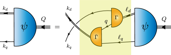
Figure 8: Figurative representation of the integral equation satisfied by the Poincaré-covariant matrix-valued function $\Psi$, viz. the Faddeev amplitude for a baryon with total momentum $Q=\ell_{q}+\ell_{d}=k_{q}+k_{d}$ built from three valence quarks, two of which are always participants in a nonpointlike, interacting diquark correlation. $\Psi$ describes the sharing of relative momentum between the dressed-quarks and -diquarks. Shaded rectangle – Faddeev kernel. Legend: single line – dressed-quark propagator, $S(q)$; $\Gamma^{J^{P}}(k;K)$ – diquark correlation amplitude; and double line – diquark propagator, $\Delta^{J^{P}}(K)$.

Given the extensive coverage of the role of diquark correlations in hadron structure presented in Ref. Barabanov et al. (2021), herein we will only draw some recent highlights from analyses of the baryon spectrum using the Faddeev equation in Fig. 8, drawing largely from Ref. Yin et al. (2021). That study was built upon a symmetry-preserving treatment of a vector$\times$vector contact interaction (SCI), which was introduced a little over a decade ago Gutiérrez-Guerrero et al. (2010) and has since been employed with success in numerous applications, some of which are reviewed in this volume Gutiérrez-Guerrero and Bashir (2022). Amongst the merits of the SCI are its algebraic simplicity; limited number of parameters; simultaneous applicability to many systems and processes; and potential for generating insights that connect and explain numerous phenomena.

Reference Yin et al. (2021) used the SCI to calculate ground-state masses of $J^{P}=0^{\pm},1^{\pm}$ $(f\bar{g})$ mesons and $J^{P}=1/2^{\pm},3/2^{\pm}$ $(fgh)$ baryons, where $f,g,h\in\{u,d,s,c,b\}$. Using $J^{P}=\tfrac{1}{2}^{\pm}$ states as exemplars, Fig. 9 highlights the level of quantitative accuracy.

Regarding the 33 mesons, then $\overline{\rm ard}=5(6)$% when comparing SCI predictions with empirical masses. In achieving this outcome, it was found that sound expressions of EHM were crucial. Turning to baryons, the SCI generated 88 distinct bound states; namely, every possible three-quark $1/2^{\pm},3/2^{\pm}$ ground-state. In this collection, 34 states have already been identified empirically and lQCD results are available for another 30: for these 64 states, comparing SCI prediction with experiment, where available, or lQCD mass otherwise, $\overline{\rm ard}=1.4(1.2)$%. This level of agreement was only achieved through implementation of EHM-induced effects associated with spin-orbit repulsion in $1/2^{-}$ baryons. Notably, the same 88 ground-states are also produced by a three-body Faddeev equation Qin et al. (2019): in comparison with those results, $\overline{\rm ard}=3.4(3.0)$%.

A
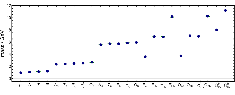
B

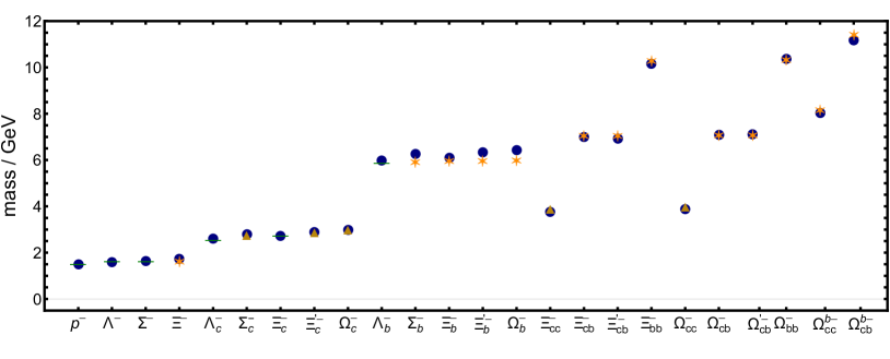
Figure 9: Upper panel – A. SCI calculated masses of ground-state flavour-SU$(5)$ $J^{P}=1/2^{+}$ baryons Yin et al. (2021) compared with either experiment (first 15) Workman et al. (2022) or lQCD (last 9) Brown et al. (2014); Mathur et al. (2018). Lower panel – B. SCI masses of ground-state flavour-SU$(5)$ $J^{P}=1/2^{-}$ baryons in Yin et al. (2021) compared with experiment Workman et al. (2022) (green bars), lQCD Bahtiyar et al. (2020) (gold triangles), or three-body Faddeev equation results Qin et al. (2019) (orange asterisks). Analogous plots for $J^{P}=3/2^{\pm}$ baryons are presented elsewhere (Yin et al., 2021, Figs. 4B, 5B).

Overall, Ref. Yin et al. (2021) delivered SCI predictions for 164 distinct quantities, 114 of which have either been measured or calculated using lQCD: performing a comparison on this subset yields $\overline{\rm ard}=4.5(7.1)$%. Such quantitative success means that credibility should be given to the qualitative conclusions that follow from the SCI analysis. We list them here. (i) Nonpointlike, dynamical diquarks play a significant role in all baryons. Usually, the lightest allowed diquark is the most important part of a baryon’s Faddeev amplitude. This remains true, even if the lightest correlation is a (sometimes called bad) axialvector diquark, and also for baryons containing one or more heavy quarks. In the latter connection, it means one cannot safely assume that singly-heavy baryons may realistically be described as two-body light-diquark+heavy-quark ($qq^{\prime}+Q$) bound-states or that doubly-heavy baryons ($qQQ^{\prime}$) can be treated as two-body light-quark+heavy-diquark bound-states, $q+QQ^{\prime}$. Corresponding statements apply to the treatment of tetra- and penta-quark problems. (ii) Positive-parity diquarks dominate in positive-parity baryons. Axialvector diquarks are prominent in all states. (iii) Negative-parity diquarks play a minor role in positive-parity baryons. On the other hand, owing to EHM, they are significant and sometimes dominant in $J=1/2^{-}$ baryons. (iv) Curiously, however, $J=3/2^{-}$ baryons are built (almost) exclusively from $J=1^{+}$ diquark correlations. These conclusions are being checked using Faddeev equations with momentum-dependent exchange interactions; hence, a closer link to QCD. Where results are already available, the SCI conclusions have been confirmed Chen et al. (2018, 2019); Liu et al. (2022a, b).

Following more than fifty years of hadron spectroscopy based on quark models, we are beginning to see real progress with the use of bound-state equations in quantum field theory. Poincaré-invariant, symmetry-preserving analyses that reveal the expressions of EHM in hadron masses and level orderings are becoming available. This increases the value of experimental hadron spectra measurements, making them a clearer window onto strong QCD.

7 Baryon Wave Functions

Concerning baryon structure, as noted when opening Sec. 6, quark models are still considered to provide a useful picture Capstick and Roberts (2000); Crede and Roberts (2013); Giannini and Santopinto (2015); Plessas (2015). In such models, baryons built from combinations of $u$, $d$, and $s$ valence quarks are grouped into multiplets of SU$(6)\otimes$O$(3)$. The multiplets are labelled by their flavour content – SU$(3)$, spin – SU$(2)$, and orbital angular momentum – O$(3)$. However, as has been emphasised, quark potential models do not have an explicit link with QCD, a Poincaré-invariant quantum gauge field theory.

For the lightest four $(I,J^{P}=\tfrac{1}{2},\tfrac{1}{2}^{\pm})$ baryons, with $I$ denoting isospin, a comparison between quark model expectations and insights drawn from solutions of the Poincaré-covariant Faddeev equation is presented elsewhere Chen et al. (2018). Herein, we will illustrate the qualitative character of such comparisons by considering more recent studies of $(\tfrac{3}{2},\tfrac{3}{2}^{\pm})$, $(\tfrac{1}{2},\tfrac{3}{2}^{\mp})$ baryons Liu et al. (2022a, b).

These systems were studied in Ref. Eichmann et al. (2016) using RL truncation and direct calculations of all primary Schwinger functions. With current algorithms, owing to singularities which enter the integration domains sampled by the Faddeev equations Maris and Roberts (1997), this approach limits the ability to compute wave functions because the on-shell point for many systems is inaccessible. (Similar issues are encountered with meson structure studies – Sec. 6.) To circumvent this issue, Refs. Liu et al. (2022a, b) employed the QCD-kindred framework introduced elsewhere Alkofer et al. (2005), in which, instead of calculating all primary Schwinger functions, one uses physics-constrained algebraic representations of the Faddeev kernel elements. This weakens the connection with QCD, but that loss is well compensated because, with reliably informed choices for the representation functions, the expedient enables access to on-shell baryon wave functions. The QCD-kindred framework has widely been used with success – see, e.g., Refs. Segovia et al. (2014); Chen et al. (2019); Lu et al. (2019); Chen et al. (2021, 2022); Chen and Roberts (2022).

Within the quark model framework and using standard spectroscopic notation, $n\,^{2S+1}\!L_{J}$, where $n$ is the radial quantum number with “0” labelling the ground state, the lightest four $(\tfrac{3}{2},\tfrac{3}{2}^{\pm})$ $\Delta$-baryons, constructed from isospin $I=\tfrac{3}{2}$ combinations of three $u$ and/or $d$ quarks, are understood as follows Klempt and Metsch (2012):

1. $\Delta(1232)\tfrac{3}{2}^{+}$ … $0\,^{4}S_{\tfrac{3}{2}}={\mathsf{S}}$-wave ground-state;

2. $\Delta(1600)\tfrac{3}{2}^{+}$ … $1\,^{4}S_{\tfrac{3}{2}}={\mathsf{S}}$-wave radial excitation of $\Delta(1232)\tfrac{3}{2}^{+}$;

3. $\Delta(1700)\tfrac{3}{2}^{-}$ … $0\,^{2}P_{\tfrac{3}{2}}={\mathsf{P}}$-wave orbital angular momentum excitation of $\Delta(1232)\tfrac{3}{2}^{+}$;

4. $\Delta(1940)\tfrac{3}{2}^{-}$ … $1\,^{4}P_{\tfrac{3}{2}}={\mathsf{P}}$-wave excitation of $\Delta(1600)\tfrac{3}{2}^{+}$.

Analogously, the $(\tfrac{1}{2},\tfrac{3}{2}^{\mp})$ states are interpreted thus Klempt and Metsch (2012):

1. $N(1520)\tfrac{3}{2}^{-}$ … $0\,^{2}P_{\tfrac{1}{2}}={\mathsf{P}}$-wave ground-state in this channel and an angular-momentum coupling partner of $N(1535)\tfrac{1}{2}^{-}$;

2. $N(1700)\tfrac{3}{2}^{-}$ … $0\,^{4}P_{\tfrac{3}{2}}={\mathsf{P}}$-wave angular-momentum coupling partner of $N(1520)\tfrac{3}{2}^{-}$;

3. $N(1720)\tfrac{3}{2}^{+}$ … $0\,^{2}D_{\tfrac{3}{2}}={\mathsf{D}}$-wave orbital angular momentum excitation of $N(1520)\tfrac{3}{2}^{-}$;

4. $N(1900)\tfrac{3}{2}^{+}$ … $0\,^{4}D_{\tfrac{3}{2}}={\mathsf{D}}$-wave orbital angular momentum excitation of $N(1700)\tfrac{3}{2}^{-}$.

On the other hand, Poincaré-invariant quantum field theory does not readily admit such assignments. Instead, the states appear as poles in the six-point Schwinger functions associated with the given $(I,J^{P})$ channels. Here, “$(1\leftrightarrow 3)$” and “$(2\leftrightarrow 4)^{\prime}$’ in each block above are related as parity partners. All differences between positive- and negative-parity states can be attributed to chiral symmetry breaking in quantum field theory. This is highlighted by the $\rho$-$a_{1}$ meson complex Weinberg (1967); Chang and Roberts (2012); Williams et al. (2016); Qin and Roberts (2021); Xu et al. (2022). Regarding light-quark hadrons, such symmetry breaking is almost exclusively dynamical Lane (1974); Politzer (1976); Pagels (1979); Higashijima (1984); Pagels and Stokar (1979); Cahill and Roberts (1985); Bashir et al. (2012). As noted above, DCSB is a corollary of EHM Roberts and Schmidt (2020); Roberts (2020, 2021); Roberts et al. (2021); Binosi (2022); Papavassiliou (2022); hence, quite probably linked tightly with confinement – Sec. 5. These features imbue quantum field theory analyses of $(\tfrac{3}{2},\tfrac{3}{2}^{\pm})$, $(\tfrac{1}{2},\tfrac{3}{2}^{\mp})$ baryons with particular interest; consequently, experiments that test predictions made for structural differences between parity partners are highly desirable.

Working with the Faddeev equation sketched in Fig. 8, then, a priori, the $(\tfrac{3}{2},\tfrac{3}{2}^{\pm})$ baryons are the simpler systems because they can only contain isovector-axialvector and isovector-vector diquarks, whereas the $(\tfrac{1}{2},\tfrac{3}{2}^{\mp})$ systems may involve all five distinct types of diquarks: $(0,0^{+})$, $(1,1^{+})$, $(0,0^{-})$, $(1,1^{-})$, $(0,1^{-})$. Nonetheless, the formulation of the bound-state problems in both channels is practically identical, using the same dressed-quark and -diquark propagators; diquark correlation amplitudes; etc. This way, one guarantees a unified description of all states in the spectrum. The propagators are parametrised using entire functions Munczek (1986); Efimov and Ivanov (1989); Burden et al. (1992); hence, satisfy the confinement constraints described in Sec. 5. It is this feature which enables on-shell calculations for all baryons.

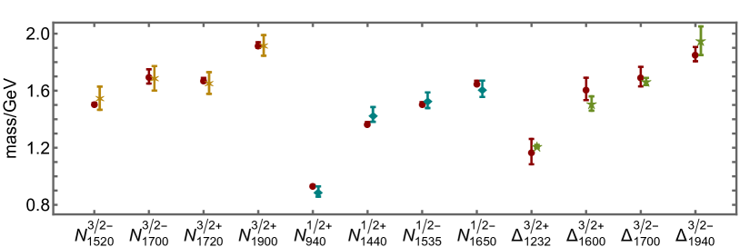
Figure 10: Real part of empirical pole position for each designated baryon Workman et al. (2022) (red circle) compared with: calculated masses in Ref. Liu et al. (2022b) (gold asterisks) after subtracting $\delta^{N_{3/2}}_{\rm MB}=0.13\,$GeV from each; Ref. Chen et al. (2018) (teal diamonds) after subtracting $\delta^{N_{1/2}}_{\rm MB}=0.30\,$GeV; and Ref. Liu et al. (2022a) (green five-pointed stars) after subtracting $\delta^{\Delta_{3/2}}_{\rm MB}=0.17\,$GeV. All Faddeev equation predictions are drawn with an uncertainty that reflects a $\pm 5$% change in diquark masses.

A		B
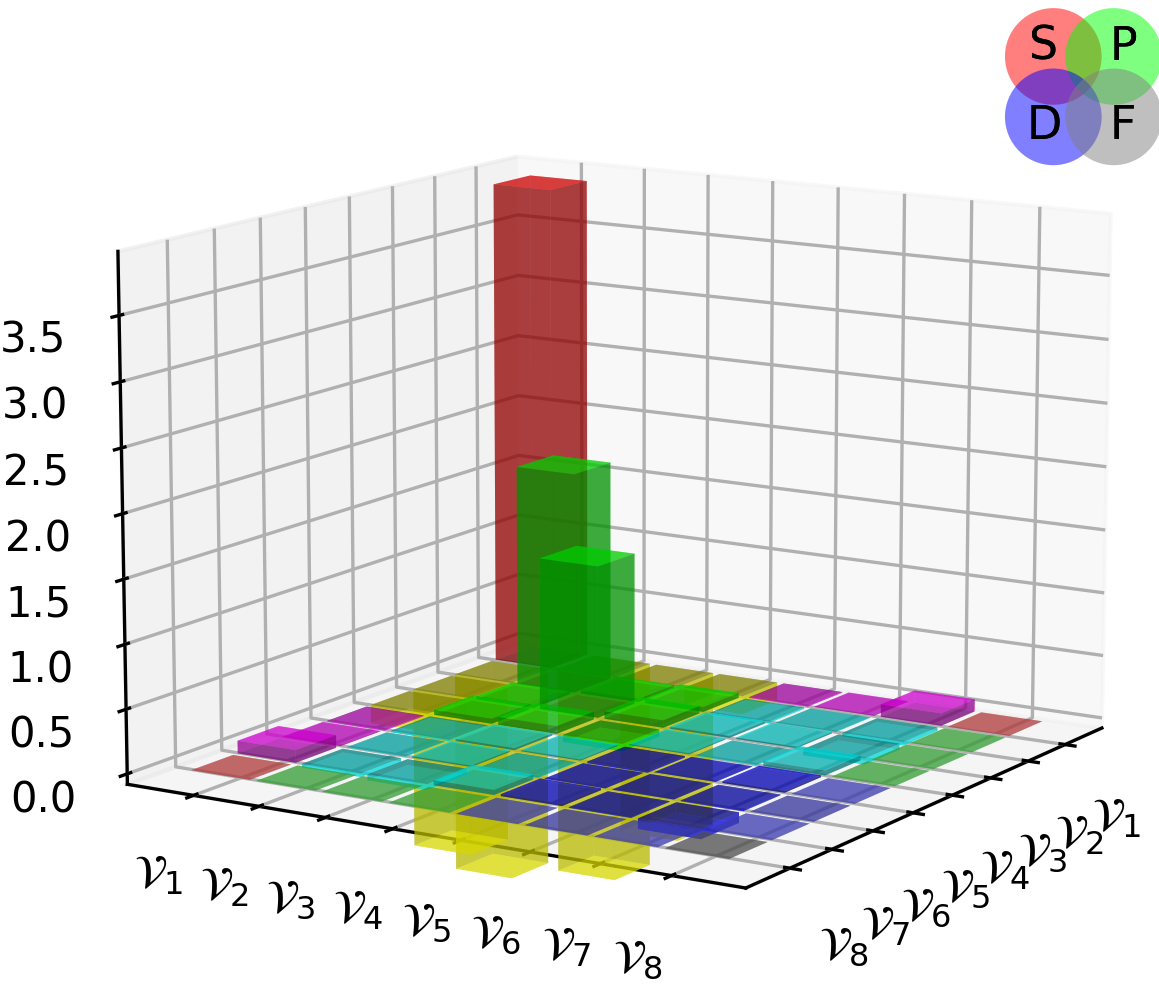
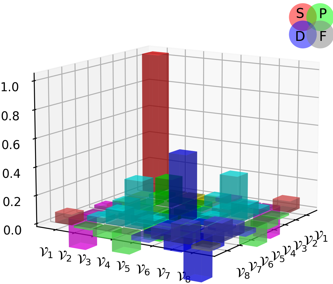
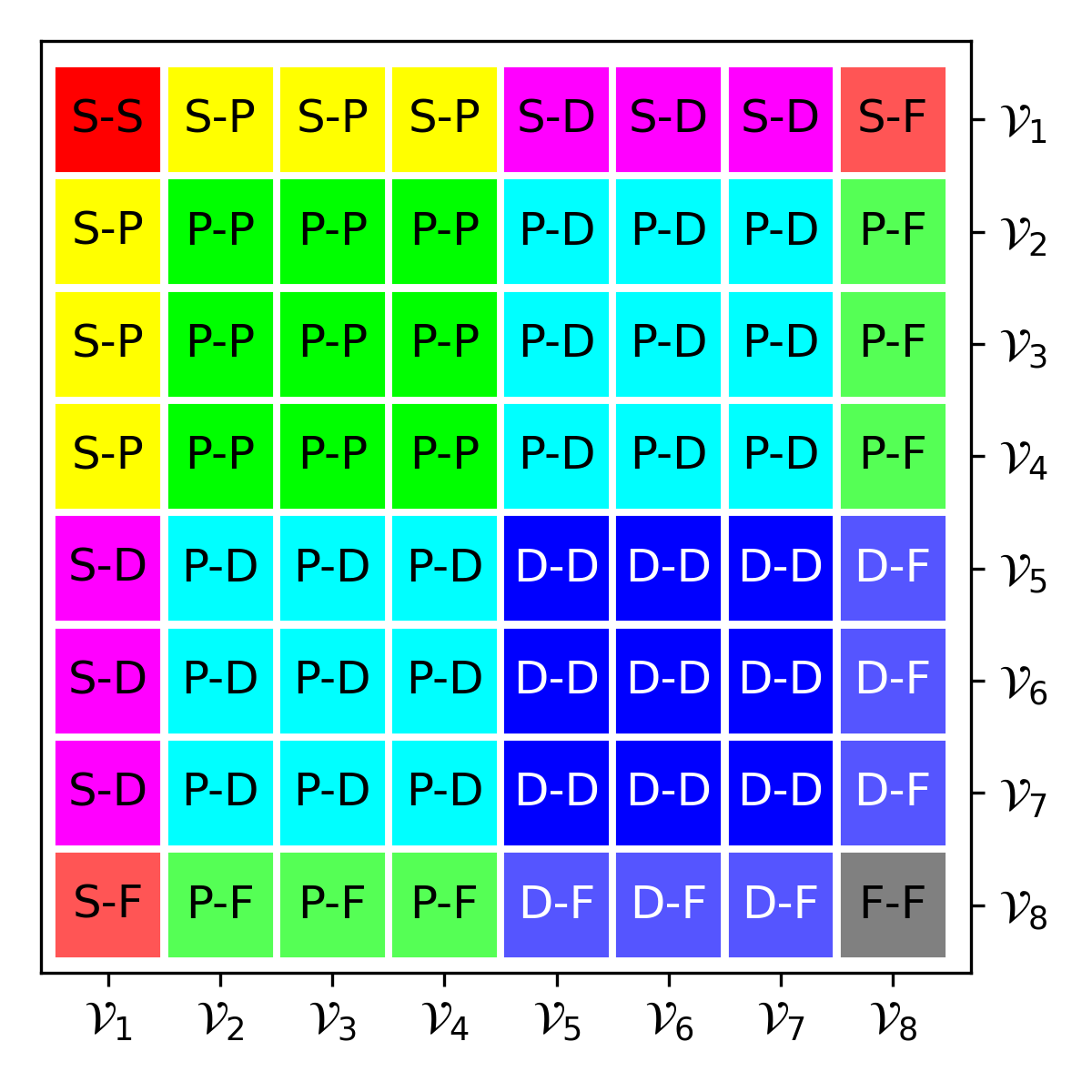
C		D

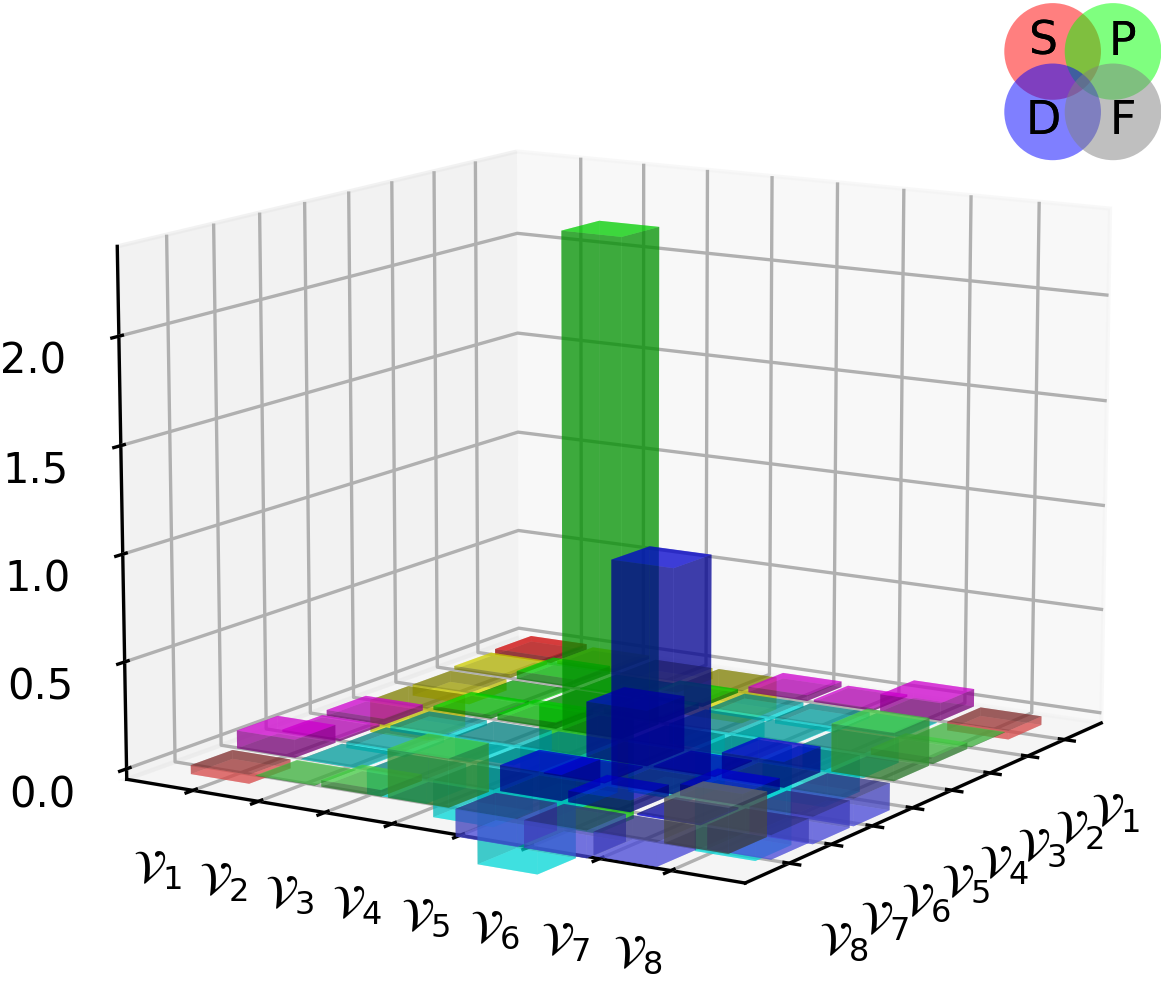
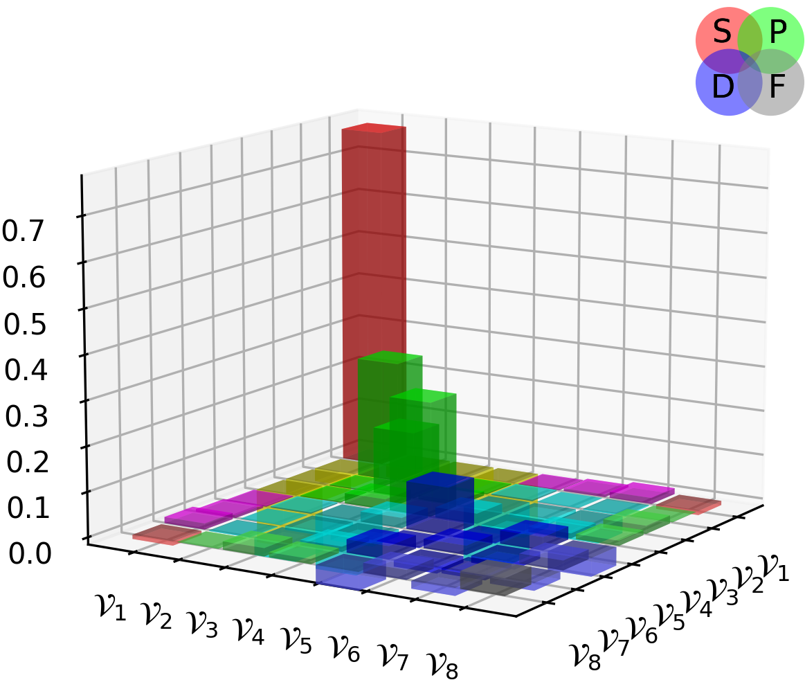
Figure 11: Rest frame quark+axialvector-diquark orbital angular momentum content of $(\tfrac{3}{2},\tfrac{3}{2}^{\pm})$ baryons considered in Ref. Liu et al. (2022a), as measured by the contribution from the various components to the associated canonical normalisation constant: A – $\Delta(1232)\tfrac{3}{2}^{+}$; B – $\Delta(1600)\tfrac{3}{2}^{+}$; C – $\Delta(1700)\tfrac{3}{2}^{-}$; and D – $\Delta(1940)\tfrac{3}{2}^{-}$. The overall-positive normalisations receive both positive (above plane) and negative (below plane) contributions. The central image provides the legend for interpretation of the other panels, identifying interference between the various identified orbital angular momentum basis components in the baryon rest frame.

The calculated spectrum of states is displayed in Fig. 10. As highlighted elsewhere Hecht et al. (2002); Sanchis-Alepuz et al. (2014); Chen et al. (2018); Burkert and Roberts (2019); Liu et al. (2022a, b), the kernel in Fig. 8 does not include contributions that may be understood as meson-baryon final-state interactions. These are the interactions which transform a bare-baryon into the observed state, e.g., via dynamical coupled channels calculations Julia-Diaz et al. (2007); Suzuki et al. (2010); Rönchen et al. (2013); Kamano et al. (2013); García-Tecocoatzi et al. (2017). The Faddeev amplitudes and masses calculated in Refs. Chen et al. (2018); Liu et al. (2022a, b) should therefore be seen as describing the dressed-quark core of the bound-state, not the fully-dressed, observable object Eichmann et al. (2008, 2009); Roberts et al. (2011). That explains why the masses are uniformly too large. Evidently and importantly, in each sector, a single subtraction constant is sufficient to realign the masses and produce a good description of the spectrum.

Regarding $(\tfrac{3}{2},\tfrac{3}{2}^{\pm})$ baryons, Ref. Liu et al. (2022a) found that although these states may contain both $(1,1^{+})$ and $(1,1^{-})$ quark+quark correlations, one can neglect the $(1,1^{-})$ diquarks because they have practically no impact on the masses or wave functions. After this simplification, the Poincaré-covariant wave functions involve eight independent matrix-valued terms, each multiplied by a scalar function of two variables: $(k^{2},k\cdot Q)$, with $k$ the quark+diquark relative momentum. Studying the properties of these functions, one may conclude that the $\Delta(1600)\tfrac{3}{2}^{+}$ is fairly interpreted as a radial excitation of the $\Delta(1232)\tfrac{3}{2}^{+}$, as suggested by the quark model. However, the wave functions of the $\Delta(1700)\tfrac{3}{2}^{-}$, $\Delta(1940)\tfrac{3}{2}^{-}$ states are complicated and do not readily admit direct analogies with quark model pictures.

Projecting the Poincaré-covariant Faddeev wave functions of $(\tfrac{3}{2},\tfrac{3}{2}^{\pm})$ baryons into their respective rest frames, one arrives at a $J=L+S$ separation which is comparable to that associated with quark models. (Here $L$ is quark-diquark orbital angular momentum.) Following this procedure, Ref. Liu et al. (2022a) found that the angular momentum structure of all these states is much more complicated than is typically generated in quark models – see Fig. 11.

Evidently, making a link to quark models, the $\Delta(1232)\tfrac{3}{2}^{+}$ and $\Delta(1600)\tfrac{3}{2}^{+}$ are characterised by a dominant $\mathsf{S}$-wave component, and the $\Delta(1700)\tfrac{3}{2}^{-}$ by a prominent $\mathsf{P}$-wave. The $\Delta(1940)\tfrac{3}{2}^{-}$, however, does not fit this picture: contrary to quark model expectations, indicated on page 4, this state is $\mathsf{S}$-wave dominated. Moreover, each state contains every admissible partial wave.

Combining all gathered information, Ref. Liu et al. (2022a) furthermore concluded that the negative parity $\Delta$-baryons are not merely orbital angular momentum excitations of positive parity ground states. In this observation, the results match those obtained earlier for $(\tfrac{1}{2},\tfrac{1}{2}^{\pm})$ baryons Chen et al. (2018).

Recalling now that the interpolating fields for positive and negative parity hadrons are related by chiral rotation of the quark spinors used in their construction, then the highlighted structural differences are largely generated by DCSB. Regarding the $\Delta(1940)\tfrac{3}{2}^{-}$ in particular, these novel structural predictions may be expected to encourage new experimental efforts aimed at extracting reliable information about this little understood state from exclusive $\pi^{+}\pi^{-}p$ electroproduction data Isupov et al. (2017); Trivedi (2019).

Observations upon similar features were made about $(\tfrac{1}{2},\tfrac{3}{2}^{\pm})$ baryons in Ref. Liu et al. (2022b). To begin, despite the fact that such states may contain all possible diquark correlations, the analyses showed that a good approximation is obtained by keeping only $(0,0^{+})$, $(1,1^{+})$ correlations. This runs counter to the nature of $(\tfrac{1}{2},\tfrac{1}{2}^{-})$ systems, in which $(0,0^{-})$, $(0,1^{-})$ diquarks are also important Chen et al. (2018); Raya et al. (2021). Projecting the Poincaré-covariant Faddeev wave functions into the baryon rest-frames and considering the baryon mass-fraction contributed by each partial wave, this collection of states form a set related via orbital angular momentum excitation: as in quark models, the parity-negative states are primarily $\mathsf{P}$-wave in nature whereas the parity-positive states are $\mathsf{D}$ wave – see Ref. (Liu et al., 2022b, Fig. 4). However, looking with finer resolution, using charts of the canonical normalisation constant contributions from the various partial waves in the Poincaré-covariant wave functions, alike with Fig. 11 herein, far greater $L$-complexity was observed than is usually found in quark models – see Ref. (Liu et al., 2022b, Fig. 7). Here, too, one may anticipate that these structural predictions can be tested using data from measurements of resonance electroexcitation at large momentum transfers. For the $N(1520)\tfrac{3}{2}^{-}$, data are already available Aznauryan et al. (2009); Mokeev et al. (2016); Mokeev (2020); Carman et al. (2020); Mokeev and Carman (2022a, b) and calculations of the electroproduction form factors are underway. Large-$Q^{2}$ data on the other states is not available; so, the predictions in Ref. Liu et al. (2022b) will also encourage new experimental efforts in this area.

Parity partner channels are identical when chiral symmetry is restored Roberts and Schmidt (2000); Fischer (2019). It is therefore interesting to note that the mass splitting between partner states does not exhibit a simple pattern, viz. empirically Workman et al. (2022):

$$\begin{array}[]{lc}{\rm states}&{\rm mass\;splitting/GeV}\\ N(1535)\tfrac{1}{2}^{-}-N(940)\tfrac{1}{2}^{+}&0.57\,,\\ N(1650)\tfrac{1}{2}^{-}-N(1440)\tfrac{1}{2}^{+}&0.29\,,\\ \Delta(1700)\tfrac{3}{2}^{-}-\Delta(1232)\tfrac{3}{2}^{+}&0.46\,,\\ \Delta(1940)\tfrac{3}{2}^{-}-\Delta(1600)\tfrac{3}{2}^{+}&0.44\,,\\ N(1720)\tfrac{3}{2}^{+}-N(1520)\tfrac{3}{2}^{-}&0.17\,,\\ N(1900)\tfrac{3}{2}^{+}-N(1700)\tfrac{3}{2}^{-}&0.22\,.\\ \end{array}$$ (27)

This system dependence of the mass splitting is also linked to the deeper structural differences between these states that are expressed in their complex wave functions.

Using a familiar quantum mechanics framework, quark models produce baryon wave functions that have an appealing simplicity. However, far richer structures are found when quantum field theory is used to solve baryon bound-state problems. The growing body of quantum field theory predictions can be tested, e.g., in modern and future large $Q^{2}$ measurements of baryon elastic and transition form factors. In fact, the large $Q^{2}$ character of such experiments is alone sufficient to demand the sort of Poincaré-invariant, symmetry-preserving treatment that only analyses in quantum field theory can deliver. One may therefore expect studies using the Faddeev equation approach outlined in this section to become steadily more widespread.

8 Meson Form Factors

The truncation scheme explained in Refs. Munczek (1995); Bender et al. (1996) has been used to calculate many meson elastic and transition form factors Maris and Roberts (2003); and modern algorithms have enabled predictions to be delivered on the entire domain of spacelike $Q^{2}$ Chang et al. (2013); Raya et al. (2016, 2017); Gao et al. (2017); Chen et al. (2018); Ding et al. (2019), making it possible to draw connections with hard scattering formulae derived using QCD perturbation theory Lepage and Brodsky (1979); Efremov and Radyushkin (1980); Lepage and Brodsky (1980). These new predictions, which unify the infrared and ultraviolet $Q^{2}$ domains, are providing the impetus for measurements at new generation high-energy and high-luminosity facilities Aguilar et al. (2019); Chen et al. (2020); Roberts et al. (2021); Arrington et al. (2021). Recalling that QCD is not found in form factor scaling but in scaling violations, then the goal of these new experiments is, of course, to discover the breakaway from scaling in a hard exclusive process and thus reveal the hand of QCD.

In connection with these new facilities, it has been argued that the interaction of a heavy vector-meson, $V=J/\psi,\Upsilon$, with a proton, $p$, may provide access to a QCD van der Waals interaction, produced by multiple gluon exchange Brodsky et al. (1990); Tarrús Castellà and Krein (2018), and/or the QCD trace anomaly Luke et al. (1992); Kharzeev (1996); Roberts (2017); Krein and Peixoto (2020). The van der Waals interaction is of interest because it might relate to, amongst other things, the observation of hidden-charm pentaquark states Aaij et al. (2015); and the trace anomaly is topical because of its connection with EHM.

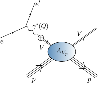
Figure 12: Electroproduction of a vector-meson from the proton: $e+p\to e^{\prime}+V+p$, often interpreted as providing access to $V+p\to V+p$ using a vector meson dominance model. The $\gamma^{(\ast)}(Q)\to V$ VMD transition is indicated by the crossed-circle. It is usually assumed to occur with a momentum-independent strength $\gamma_{\gamma V}$ Sakurai (1960, 1969); Fraas and Schildknecht (1969). However, regarding heavy mesons, at least, the VMD hypothesis is unsound, as discussed below and in, e.g., Refs. Xu et al. (2021); Sun et al. (2022).

Lacking vector-meson beams, ongoing and anticipated experiments at electron ($e$) accelerators are based on an expectation that the desired $V+p$ interactions can be accessed through the electromagnetic production of vector-mesons from the proton, in reactions like $e+p\to e^{\prime}+V+p$ Ali et al. (2019); Anderle et al. (2021); Abdul Khalek et al. (2022). This is because some practitioners imagine that single-pole vector meson dominance (VMD) Sakurai (1960, 1969); Fraas and Schildknecht (1969) can reliably be employed to draw a clean link between $e+p\to e^{\prime}+V+p$ and the desired $Vp\to Vp$ cross-sections. In this picture – see Fig. 12, the interaction is supposed to proceed via the following sequence of steps: (i) $e\to e^{\prime}+\gamma^{(\ast)}(Q)$; (ii) $\gamma^{(\ast)}(Q)\to V$; and (iii) $V+p\to V+p$. $\gamma^{(\ast)}(Q)$ is a virtual photon and step (ii) expresses the VMD hypothesis. As commonly used, VMD assumes: (a) that a photon, which is generally spacelike, so that $Q^{2}>0$, transforms into an on-shell vector-meson, with timelike momentum $Q^{2}=-m_{V}^{2}$; and (b) that the $Q^{2}>0$ strength and form of the transition in (ii) is the same as that measured in the real vector meson decay process, $V\to\gamma^{\ast}(Q^{2}=-m_{V}^{2})\to e^{+}+e^{-}$. Property (b) means that $\gamma_{\gamma V}$, the associated decay constant, is fixed at its meson on-shell value and acquires no momentum dependence:

$$\gamma_{\gamma V}^{2}=4\pi\alpha_{\rm em}m_{V}^{2}f_{V}^{2}\,,$$ (28)

where $\alpha_{\rm em}$ is the QED fine-structure constant, $m_{V}$ is the vector meson mass, and $f_{V}$ measures the strength of the meson’s Bethe-Salpeter wave function at the origin in configuration space (Ivanov et al., 1999, Sec. IIB).

The fidelity of these VMD assumptions was recently subjected to scrutiny via analyses of the photon vacuum polarisation and photon-quark vertex Xu et al. (2021). Regarding the photon vacuum polarisation, it was shown that there is no vector-meson contribution to this polarisation at the photoproduction point, $Q^{2}=0$. Consequently, massless real photons cannot readily be linked with massive vector-bosons and the current-field identity, Eq. (28), typical of VMD implementations, should not be used literally because it entails violations of Ward-Green-Takahashi identities (breaking of symmetries) in QED.

A		B

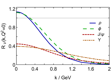
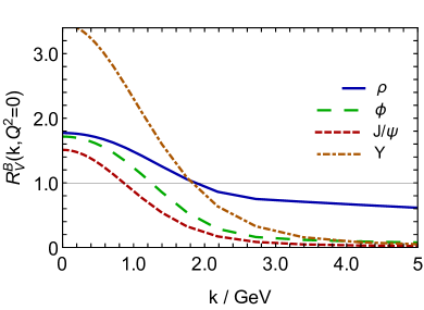
Figure 13: Left panel – A: First ratio in Eq. (29) computed using matched solutions of the gap and Bethe-Salpeter equations for $V=\rho,\phi,J/\psi,\Upsilon$. Right panel – B: Second ratio in Eq. (29), computed similarly. In cases where the VMD hypothesis were sound, all these curves would lie close to the thin horizontal line drawn at unity.

Turning to the dressed photon-quark vertex, $\Gamma_{\nu}^{\gamma}(k;Q)$, this three-point Schwinger function exhibits a pole at the mass of any vector-meson bound-state. A physical property, it expresses the fact that the decay $V\to e^{+}e^{-}$ proceeds via a timelike virtual photon. The VMD hypothesis may thus be seen as a claim that $\left.\Gamma_{\nu}^{\gamma}(k;Q)\right|_{Q^{2}\simeq 0}$ maintains a rigorous link, in both magnitude and momentum-dependence, with the Bethe-Salpeter amplitude of an on-shell vector-meson. However, as shown in Fig. 13, that is not the case. The panels in Fig. 13 depict the ratios

$$R_{V}(k^{2};Q^{2}=0)=\frac{2f_{V}}{m_{V}}\frac{F_{1}^{0}(k^{2};-m_{V}^{2})}{G_{1}^{0}(k^{2};Q^{2}=0)}\,,\quad R_{V}^{B}(k^{2};Q^{2}=0)=\frac{f_{V}}{m_{V}}\frac{F_{8}^{0}(k^{2};-m_{V}^{2})}{G_{3}^{0}(k^{2};Q^{2}=0)}\,,$$ (29)

where $G_{1}^{0}$ is the zeroth Chebyshev moment of the dominant amplitude in the photon-quark vertex, associated with the matrix structure $\gamma\cdot\epsilon(Q)$, where $\epsilon(Q)$ is the photon polarisation vector – in fact, using the vector Ward-Green-Takahashi identity and Eq. (23), $G_{1}^{0}(k^{2};Q^{2}=0)=A_{g}(k^{2})$, where $g$ is the flavour of the meson’s valence quark; $F_{1}^{0}$ is its analogue in the vector meson bound-state amplitude; $G_{3}^{0}$ is the zeroth moment of that term in the photon-quark vertex which is directly linked to the scalar piece of the dressed-quark self-energy via the vector Ward-Green-Takahashi identity, i.e., $G_{3}^{0}(k^{2};Q^{2}=0)=-2B_{g}^{\prime}(k^{2})$; and $F_{8}^{0}$ is its analogue in the vector meson bound-state amplitude. Were VMD to be a sound assumption, then all these curves would lie near to the thin horizontal line drawn at unity in both panels of Fig. 13. However, whilst one might discuss the case for lighter vector mesons, the VMD hypothesis is plainly false for heavy vector mesons: the momentum-dependence of the $Q^{2}=0$ photon-quark vertex is completely different from that of the vector-meson Bethe-Salpeter amplitude.

One is consequently led to conclude that insofar as heavy mesons are concerned, no extant attempt to link $e+p\to e^{\prime}+V+p$ reactions with $V+p\to V+p$ via VMD is reliable. A similar conclusion is drawn in Ref. Sun et al. (2022) using arguments within perturbative QCD. It is strengthened by Ref. Du et al. (2020), which demonstrates that even if VMD were valid, then contributing relevant coupled-channels processes would obscure connections between $e+p\to e^{\prime}+V+p$ and $V+p\to V+p$ reactions. These analyses make tenuous any interpretation of $e+p\to e^{\prime}+V+p$ reactions as a path to hidden-charm pentaquark production or as a route to understanding the origin of the proton mass. In fact, the crudity of existing models prevents sound conclusions being drawn about the capacity of heavy meson production to reveal something about the SM Lee et al. (2022).

On the other hand, numerous applications Eichmann et al. (2016); Roberts and Schmidt (2020); Eichmann et al. (2020); Roberts (2020); Qin and Roberts (2020), including $\gamma^{\ast}\gamma\to\pi^{0}$, $\eta$, $\eta^{\prime}$, $\eta_{c}$, $\eta_{b}$ Raya et al. (2017); Ding et al. (2019), show that a viable alternative to the VMD hypothesis exists in adapting the CSMs discussed herein to a direct analysis of processes like $\gamma^{(\ast)}+p\to V+p$. Considering vector-meson photo/electroproduction from the proton, Refs. Pichowsky and Lee (1997); Shi et al. (2021); Lee et al. (2022) illustrate how one might proceed; and given developments in the past vicennium, improvements of such studies are now possible.

Following the first studies almost thirty years ago Roberts (1996), the CSM treatment of meson elastic and transition form factors has now reached a mature level. Today, as sketched above, sound predictions with a traceable connection to QCD are being delivered. This enables new opportunities to be exploited, such as informative comparison with results from lQCD Chen et al. (2018), weak transitions of heavy mesons – see Refs. Yao et al. (2020, 2021, 2022) and Sec. 10, calculations of form factors describing light-by-light scattering contributions to the muon anomalous magnetic moment Miramontes et al. (2022), and a beginning to the analysis of meson gravitational form factors Rodríguez-Quintero (2022).

9 Baryon Form Factors

Advances in the calculation of meson form factors are complemented by progress with the parameter-free prediction of baryon elastic and transition form factors. The first direct RL truncation study of nucleon elastic form factors was presented in Ref. Eichmann (2011). It was extended to nucleon axial and pseudoscalar form factors in Ref. Eichmann and Fischer (2012), the elastic form factors of $\Delta$- and $\Omega$-baryons in Ref. Sanchis-Alepuz et al. (2013), and nucleon tensor charges in Ref. Qin and Roberts (2020).

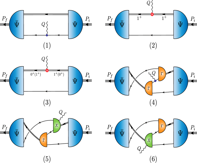
Figure 14: Axial/pseudoscalar current that ensures a symmetry-preserving interaction with an on-shell baryon described by a Faddeev amplitude obtained from the equation depicted in Fig. 8: single line, dressed-quark propagator; undulating line, axial/pseudoscalar current; $\Gamma$, diquark correlation amplitude; double line, diquark propagator; and $\chi$, seagull terms. A detailed legend is provided in Table 2.

Many other direct RL truncation analyses are in train. However, in all such studies, the challenge of quark propagator singularities moving into the complex integration domain must also be overcome Maris and Roberts (1997). Using existing algorithms, the singularities limit the $Q^{2}$-reach of baryon form factor calculations. Here, again, the QCD-kindred quark plus fully-interacting, nonpointlike diquark picture of baryon structure – outlined in Sec. 7 – can profitably be exploited. Some of the successes are summarised elsewhere Brodsky et al. (2020); Barabanov et al. (2021). Recently, the predictions made for $\gamma+p\to\Delta(1600)$ transition form factors Lu et al. (2019) have been tested in analyses of $\pi^{+}\pi^{-}p$ electroproduction data collected at Jefferson Lab (JLab) Mokeev (2022a), with preliminary results supporting the quark+diquark picture Mokeev (2022b).

Scanning the sources indicated above, it becomes apparent that, hitherto, nucleon properties have largely been probed in $e+N$ scattering. Aspects of this field are reviewed elsewhere Perdrisat et al. (2007). An entirely new window onto baryon structure is opened when one uses neutrino scattering. In fact, reliable predictions of nucleon and $N\to\Delta(1232)$ electroweak form factors are crucial for understanding new-generation long-baseline neutrino oscillation experiments Mosel (2016); Alvarez-Ruso et al. (2018); Hill et al. (2018); Gysbers et al. (2019); Lovato et al. (2020); King et al. (2020); Simons et al. (2022). Importantly in this connection, recent developments within the framework of CSMs have enabled practitioners to deliver the first Poincaré-invariant parameter-free predictions for such form factors on a momentum transfer domain that extends to $Q^{2}=10\,$GeV² Chen et al. (2021, 2022); Chen and Roberts (2022). Extensions to even larger $Q^{2}$ are feasible. Where data are available, the predictions confirm the measurements. More significantly, the results are serving as motivation for new experiments at high-luminosity facilities.

Table 2: Enumeration of terms in the baryon axialvector/pseudoscalar current, drawn in Fig. 14.

1. Diagram 1, two terms: $\langle J\rangle^{S}_{\rm q}$ – probe strikes dressed-quark with scalar diquark spectator; and $\langle J\rangle^{A}_{\rm q}$ – probe strikes dressed-quark with axialvector diquark spectator.

2. Diagram 2: $\langle J\rangle^{AA}_{\rm qq}$ – probe strikes axialvector diquark with dressed-quark spectator.

3. Diagram 3: $\langle J\rangle^{\{SA\}}_{\rm qq}$ – probe mediates transition between scalar and axialvector diquarks, with dressed-quark spectator.

4. Diagram 4, three terms: $\langle J\rangle_{\rm ex}^{SS}$ – probe strikes dressed-quark “in-flight” between one scalar diquark correlation and another; $\langle J\rangle_{\rm ex}^{\{SA\}}$ – dressed-quark “in-flight” between a scalar diquark correlation and an axialvector correlation; and $\langle J\rangle_{\rm ex}^{AA}$ – “in-flight” between one axialvector correlation and another.

5. Diagrams 5 and 6 – seagull diagrams describing the probe coupling into the diquark correlation amplitudes: $\langle J\rangle_{\rm sg}$. There is one contribution from each diagram to match every term in Diagram (4).

The key step in the use of CSMs was construction of a symmetry-preserving current that describes the coupling between axialvector and pseudoscalar probes and baryons whose structure is determined by the Faddeev equation in Fig. 8. This current is illustrated in Fig. 14 and explained by the legend in Table 2. The origins and characters of Diagrams 1-3 are obvious: the probe must interact with every “constituent” that carries a weak charge. Diagram 4 is a two-loop diagram, made necessary by the quark-exchange nature of the kernel in Fig. 8: the object exchanged in binding also carries a weak charge. Given the presence of Diagram 4, so-called seagull diagrams – Diagrams 5 and 6 – are necessary to ensure symmetry preservation. The analogous contributions for baryon electromagnetic currents were derived in Ref. Oettel et al. (2000), but it took more than twenty years before the seagull terms were derived for axialvector and pseudoscalar currents Chen et al. (2022). These contributions are both two-loop diagrams.

Axialvector interactions of a nucleon are described by two form factors – $G_{A}(Q^{2})$ (axial) and $G_{P}(Q^{2})$ (induced-pseudoscalar), associated with the following matrix element:

$$\hat{J}^{j}_{5\mu}(K,Q) :=\langle N(P_{f})|{\mathpzc A}^{j}_{5\mu}(0)|N(P_{i})\rangle$$ (30a)

$$= \bar{u}(P_{f})\frac{\tau^{j}}{2}\gamma_{5}\bigg{[}\gamma_{\mu}G_{A}(Q^{2})+i\frac{Q_{\mu}}{2m_{N}}G_{P}(Q^{2})\bigg{]}\,u(P_{i})\,,$$ (30b)

where $P_{i,f}$ are, respectively, the initial and final nucleon momenta, with $P_{i,f}^{2}=-m_{N}^{2}$, $m_{N}$ is the nucleon mass, and $u(P)$ is the associated Euclidean spinor. (Associated conventions are specified elsewhere, e.g., Ref. (Segovia et al., 2014, Appendix B).) The average momentum of the system is $K=(P_{i}+P_{f})/2$ and $Q=P_{f}-P_{i}$ is the momentum transferred between initial and final states. It is usual to consider the SU$(2)_{\rm F}$ isospin limit $m_{u}=m_{d}=:m_{q}$, with the flavour structure described using Pauli matrices $\{\tau^{j}|j=1,2,3\}$: $\tau^{1\pm i2}:=(\tau^{1}\pm i\tau^{2})/2$ correspond to the weak charged currents and $\tau^{3}$ is the neutral current. Moreover, the isovector axial current operator is

$${\mathpzc A}_{5\mu}^{j}(x)=\bar{q}(x)\frac{\tau^{j}}{2}\gamma_{5}\gamma_{\mu}q(x),\,\,\,\,\,q=\left(\begin{array}[]{c}u\\ d\end{array}\right)\,.$$ (31)

A third form factor is defined via the kindred pseudoscalar current, a matrix element of ${\mathpzc P}^{j}_{5}(x)=\bar{q}(x)\frac{\tau^{j}}{2}\gamma_{5}q(x)$:

$$\hat{J}^{j}_{5}(K,Q):=\langle N(P_{f})|{\mathpzc P}^{j}_{5}(0)|N(P_{i})\rangle=\bar{u}(P_{f})\frac{\tau^{j}}{2}\gamma_{5}\,G_{5}(Q^{2})\,u(P_{i})\,.$$ (32)

Using the framework deployed to calculate the baryon wave functions discussed in Sec. 7, Refs. Chen et al. (2021, 2022) delivered the parameter-free prediction for $G_{A}(Q^{2})$ displayed in Fig. 15: the lighter blue band expresses the impact of $\pm 5$% variations in the diquark masses: $m_{0^{+}}=0.80(1\pm 0.05)$; $m_{1^{+}}=0.89(1\pm 0.05)$. The calculated values for the nucleon axial charge $g_{A}=G_{A}(Q^{2}=0)$, associated axial charge radius, and axial mass are, respectively,

$$g_{A}=1.25(3)\,,\quad\langle r^{2}_{A}\rangle^{1/2}m_{N}=3.25(4)\,,\quad m_{A}/m_{N}=1.23(3)\,.$$ (33)

For comparison, empirically $g_{A}=1.2756(13)$ (Workman et al., 2022, PDG) and Meyer et al. (2016) $\langle r^{2}_{A}\rangle^{1/2}m_{N}=3.23(72)$, $m_{A}/m_{N}=1.15(08)$. Evidently, the CSM predictions agree with extant data. Regarding the axial mass, we note that it is sometimes convenient, when comparing with other analyses, to use a dipole Ansatz as an approximation for the axial form factor:

$$G_{A}(Q^{2})=\frac{g_{A}}{\big{(}1+Q^{2}/m_{A}^{2}\big{)}^{2}}\,;$$ (34)

so Refs. Chen et al. (2021, 2022) extracted $m_{A}$ using Eq. (34) to interpolate the global $Q^{2}$-behaviour of $G_{A}$ on $x\in[0,1.6]$, in which case $m_{A}$ is not simply related to the axial radius. It is worth remarking that scalar and axialvector diquark mass variations interfere destructively, e.g., reducing $m_{0^{+}}$ increases $g_{A}$, whereas $g_{A}$ decreases with the same change in the axialvector mass.

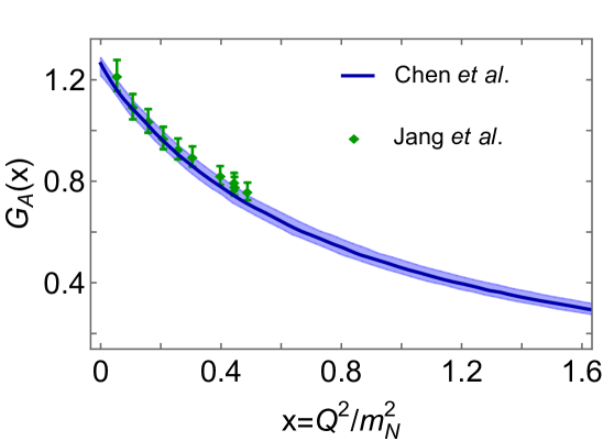
Figure 15: Predicted result for $G_{A}(x)$ in Ref. (Chen et al., 2022, Chen et al.) – blue curve within lighter blue uncertainty band, compared with lQCD results from Ref. (Jang et al., 2020, Jang et al.) – green diamonds. With respect to the CSM central results, this comparison may be quantified by reporting the mean-$\chi^{2}$ value, which is 0.27.

Turning to the induced pseudoscalar form factor, muon capture experiments ($\mu\,+\,p\,\to\,\nu_{\mu}\,+\,n$) may be used to determine the induced pseudoscalar charge:

$$g_{p}^{\ast}=\frac{m_{\mu}}{2m_{N}}G_{P}(Q^{2}=0.88\,m_{\mu}^{2})\,.$$ (35)

The CSM prediction is $g_{p}^{\ast}=8.80(23)$. Compared with the recent MuCap Collaboration result, $g_{p}^{\ast}=8.06(55)$ Andreev et al. (2013, 2015), it agrees within uncertainties but is slightly larger. The CSM value is nicely aligned with the world average Bernard et al. (2002): $g_{p}^{\ast}=8.79(1.92)$.

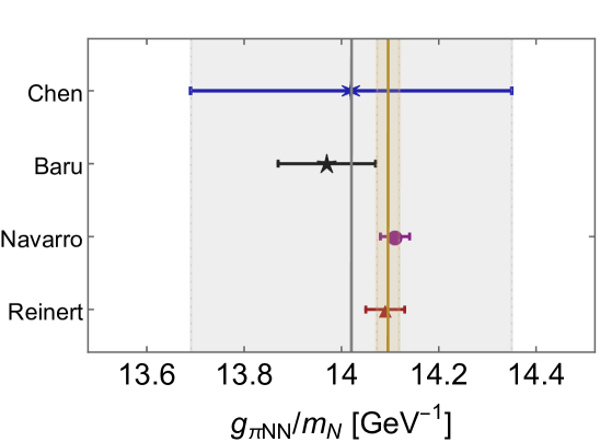
Figure 16: Comparison of the CSM prediction for $g_{\pi NN}/m_{N}$ (blue asterisk) Chen et al. (2022) with values extracted from pion-nucleon scattering (Baru et al., 2011, Baru) (black star), Granada 2013 $np$ and $pp$ scattering database (Navarro Pérez et al., 2017, Navarro) (purple circle), and nucleon-nucleon scattering (Reinert et al., 2021, Reinert) (red triangle). The vertical grey band marks the estimated uncertainty in the CSM prediction. The error-weighted average of the depicted results, Eq. (37), is drawn as the gold line within like-coloured band.

The pseudoscalar form factor, $G_{5}(Q^{2})$, is of interest because, inter alia, it is used to define the pion-nucleon form factor $G_{\pi NN}(Q^{2})$ via

$$G_{5}(Q^{2})=:\frac{m_{\pi}^{2}}{Q^{2}+m_{\pi}^{2}}\frac{f_{\pi}}{m_{q}}G_{\pi NN}(Q^{2})\,,$$ (36)

where $f_{\pi}$ is the pion leptonic decay constant (appearing in Fig. 7) and $G_{\pi NN}(-m_{\pi}^{2})=g_{\pi NN}$ is the $\pi NN$ coupling, a key input to nucleon+nucleon potentials. The CSM prediction is Chen et al. (2021, 2022): $g_{\pi NN}/m_{N}=14.02(33)/{\rm GeV}$. This value overlaps with that inferred from pion-nucleon scattering Baru et al. (2011) ($g_{\pi NN}/m_{N}=13.97(10)/{\rm GeV}$); and compares favourably with a determination based on the Granada 2013 $np$ and $pp$ scattering database Navarro Pérez et al. (2017) ($g_{\pi NN}/m_{N}=14.11(3)/{\rm GeV}$) and a recent analysis of nucleon-nucleon scattering using effective field theory and related tools Reinert et al. (2021) ($g_{\pi NN}/m_{N}=14.09(4)/{\rm GeV}$). All these results are compared in Fig. 16, which also highlights their error-weighted average:

$$g_{\pi NN}/m_{N}=14.10(2)/{\rm GeV}\,.$$ (37)

Continuing with an effort to inform nuclear physics potentials using hadron physics results, it is worth noting that on $-m_{\pi}^{2}<Q^{2}<2\,m_{N}^{2}$, a fair approximation to the CSM prediction for the pion-nucleon form factor is provided by $(x=Q^{2}/m_{N}^{2})$:

$$G_{\pi NN}^{d}(x)=\frac{13.47m_{N}}{(1+x/0.845^{2})^{2}}\,.$$ (38)

This corresponds to a $\pi NN$ dipole mass $\Lambda_{\pi NN}=0.845m_{N}=0.79\,$GeV, viz. a soft form factor. (A commensurate value was obtained previously in a simpler quark+scalar-diquark model Bloch et al. (2000).) Being just $\sim 20$% greater, the CSM prediction is qualitatively equivalent to the $\pi NN$ dipole mass inferred in a dynamical coupled-channels analysis of $\pi N$, $\gamma N$ interactions Kamano et al. (2013). Future such coupled channels studies may profit by implementing couplings and range parameters determined in CSM analyses.

An extension of this effort to the more general case of hyperon+nucleon potentials can be found in Ref. Cheng et al. (2022). Using a SCI, predictions were made therein for an array of meson+octet-baryon couplings. Comparing the results with extant phenomenological interactions Haidenbauer and Meissner (2005); Rijken et al. (2010); Kamano et al. (2013), one finds a mean absolute relative deviation ($P$ is the pseudoscalar meson absorbed in the baryon transition $B\to B^{\prime}$ and $g_{PB^{\prime}B}$ is the associated coupling)

$$\delta_{r}^{g}:=\{|g_{PB^{\prime}B}^{\rm SCI}/g_{PB^{\prime}B}^{\mbox{\rm\footnotesize phen.}}-1|\}=0.18(14)\,.$$ (39)

This result strengthens the case in favour of using CSM predictions for the couplings as new constraints in the development of baryon+baryon potentials.

A little algebra reveals that the proton axial charge can be interpreted as a measure of the valence-quark contributions to the proton light-front helicity, e.g., Ref. (Chang et al., 2013, Eqs. (6)–(8)):

$$g_{A}=\int_{0}^{1}dx\,[\Delta{\mathpzc u}^{p}(x;\zeta_{\cal H})-\Delta{\mathpzc d}^{p}(x;\zeta_{\cal H})]=:g_{A}^{u}-g_{A}^{d}\,,$$ (40)

where $\Delta{\mathpzc q}^{p}(x;\zeta_{\cal H})={\mathpzc q}^{p}_{\uparrow}(x;\zeta_{\cal H})-{\mathpzc q}^{p}_{\downarrow}(x;\zeta_{\cal H})$ is the light-front helicity DF for a quark $q$. Plainly, $\Delta{\mathpzc q}^{p}$ is the difference between the light-front number-density of quarks with helicity parallel and antiparallel to that of the proton. It is scale dependent.

Eq. (40) conveys additional significance to a flavour separation of the axial charge form factor:

$$G_{A}(Q^{2})=G_{A}^{u}(Q^{2})-G_{A}^{d}(Q^{2})\,.$$ (41)

A detailed analysis is presented in Ref. (Chen and Roberts, 2022, Sec. 4), which reveals the following diagram contributions to the separate $u$, $d$ axial form factors:

$$G_{A}^{u} =\langle J\rangle^{S}_{\rm q}-\mbox{\text@underline{$\langle J\rangle^{A}_{\rm q}$}}+\langle J\rangle^{AA}_{\rm qq}+\tfrac{1}{2}\langle J\rangle^{\{SA\}}_{\rm qq}+2\langle J\rangle^{\{SA\}}_{\rm ex}+\tfrac{4}{5}\langle J\rangle^{AA}_{\rm ex},$$ (42a)

$$-G_{A}^{d} =\phantom{\langle J\rangle^{S}_{\rm q}-}\mbox{\text@underline{$2\langle J\rangle^{A}_{\rm q}$}}+\tfrac{1}{2}\langle J\rangle^{\{SA\}}_{\rm qq}+\langle J\rangle^{SS}_{\rm ex}-\langle J\rangle^{\{SA\}}_{\rm ex}+\tfrac{1}{5}\langle J\rangle^{AA}_{\rm ex},$$ (42b)

where the nomenclature of Table 2 is used. Identified according to Eqs. (42), the calculated $Q^{2}=0$ contributions are listed in Table 3. It is worth stressing that Eqs. (42) express the fact that since a $0^{+}$ diquark cannot couple to an axialvector current, then Diagram 1 in Fig. 14 only supplies a $u$-quark contribution to the proton $G_{A}(Q^{2})$, viz. $\langle J\rangle^{S}_{\rm q}$. It follows that in a scalar-diquark-only proton, a $d$-quark contribution to $G_{A}(Q^{2})$ can only arise from Fig. 14 - Diagram 4, i.e., $\langle J\rangle^{SS}_{\rm ex}$; and $|\langle J\rangle^{SS}_{\rm ex}/\langle J\rangle^{S}_{\rm q}|\approx 0.06$. Notably, many scalar-diquark-only models omit Diagram 4, in which cases $G_{A}^{d}(Q^{2})\equiv 0$. An extension of these observations to the complete array of octet baryons is described elsewhere (Cheng et al., 2022, Sec. IV).

Table 3: Flavour and diagram – Fig. 14 – separation of the proton axial charge: $g_{A}^{u}=G_{A}^{u}(0)$, $g_{A}^{d}=G_{A}^{d}(0)$; $g_{A}^{u}-g_{A}^{d}=1.25(3)$. The listed uncertainties express the effect of $\pm 5$% variations in the diquark masses, e.g. $0.88_{6_{\mp}}\Rightarrow 0.88\mp 0.06$.

	$\langle J\rangle^{S}_{\rm q}$	$\langle J\rangle^{A}_{\rm q}$	$\langle J\rangle^{AA}_{\rm qq}$	$\langle J\rangle^{\{SA\}}_{\rm qq}$	$\langle J\rangle_{\rm ex}^{SS}$	$\langle J\rangle_{\rm ex}^{\{SA\}}$	$\langle J\rangle_{\rm ex}^{AA}$
$g_{A}^{u}$	$0.88_{6_{\mp}}$	$-0.08_{0_{\pm}}$	$0.03_{0_{\pm}}$	$0.08_{0_{\mp}}$	$0$	$\approx 0$	$0.03_{1_{\pm}}$
$-g_{A}^{d}$	$0$	$\phantom{-}0.16_{0_{\pm}}$	$0$	$0.08_{0_{\mp}}$	$0.05_{1_{\pm}}$	$\approx 0$	$0.01_{0_{\pm}}$

Using the solution of the Faddeev equation – Fig. 8, Ref. Chen and Roberts (2022) reports

$$g_{A}^{u}/g_{A}=\phantom{-}0.76\pm 0.01\,,\quad g_{A}^{d}/g_{A}=-0.24\pm 0.01\,,\quad g_{A}^{d}/g_{A}^{u}=-0.32\pm 0.02\,.$$ (43)

In nonrelativistic quark models with uncorrelated wave functions, $g_{A}^{d}/g_{A}^{u}=-1/4$. Hence, the relevant comparison reveals that the highly-correlated wave function obtained by solving the Faddeev equation gives the valence $d$ quark a markedly larger fraction of the proton’s light-front helicity than is found in simple quark models. Reviewing the discussion after Eq. (42), it becomes apparent that this feature owes to the presence of axialvector diquarks in the proton: the current contribution arising from the $\{uu\}$ correlation – underlined term in Eq. (42b), measuring the probe striking the valence $d$ quark, is twice as strong as that from the $\{ud\}$ correlation – underlined term in Eq. (42a), in which the probe strikes the valence $u$ quark.

It is natural to enquire after the robustness of the results in Eq. (43). Consider, therefore, that assuming SU$(3)$-flavour symmetry in analyses of octet baryon axial charges, these charges are expressed in terms of two low-energy constants, (Cabibbo et al., 2003, Table 1): $D$, $F$, with $g_{A}^{u}=2F$, $g_{A}^{d}=F-D$. (This assumption is accurate to roughly 4% – see, e.g., Ref. Cheng et al. (2022).) In this case, the values in Eq. (43) correspond to

$$D=0.78(2)\,,\quad F=0.48(1)\,,\quad F/D=0.61(2)\,.$$ (44)

On the other hand, using available empirical information Workman et al. (2022), one obtains $D=0.774(26)$, $F=0.503(27)$, and $g_{A}^{u}/g_{A}=0.79(4)$, $g_{A}^{d}/g_{A}=-0.21(3)$, $g_{A}^{d}/g_{A}^{u}=-0.27(4)$, values which are consistent with the results in Eqs. (43), (44). In addition, the SCI predicts Cheng et al. (2022)

$$D=0.78\,,\;F=0.43\,,\;F/D=0.56\,,$$ (45)

and a covariant baryon chiral perturbation theory analysis yields $D=0.80(1)$, $F=0.47(1)$, $F/D=0.59(1)$ Ledwig et al. (2014).

Given the favourable realistic proton wave function comparisons presented above, the values in Eq. (43) can be viewed as reliable. This is important because of the connection between flavour-separated axial charges and the so-called proton “spin crisis” Aidala et al. (2013); Deur et al. (2019). At any given resolving scale, the singlet, triplet, and octet axial charges of the proton are, respectively:

$$a_{0}=g_{A}^{u}+g_{A}^{d}+g_{A}^{s}\,,\quad a_{3}=g_{A}=g_{A}^{u}-g_{A}^{d}\,,\quad a_{8}=g_{A}^{u}+g_{A}^{d}-2g_{A}^{s}\,.$$ (46)

If working at the hadron scale, $\zeta_{\cal H}$, where dressed valence quasiparticles carry all proton properties Cui et al. (2021, 2020, 2022a, 2022b); Chang et al. (2022); Lu et al. (2022), then $g_{A}^{s}\equiv 0$ $a_{0}=a_{8}$; hence Chen and Roberts (2022)

$$a_{0}=0.65(2)\,.$$ (47)

In general, $a_{3,8}$ are conserved charges, viz. they are the same at all resolving scales, $\zeta$. However, that is not true of the individual terms in their definitions: the separate valence quark charges $g_{A}^{u}$, $g_{A}^{d}$, $g_{A}^{s}$ evolve with $\zeta$ Deur et al. (2019). Consequently, the value of $a_{0}$, which is the fraction of the proton’s total $J=1/2$ carried by valence degrees-of-freedom, changes with scale: the result in Eq. (47) is the maximum value of $a_{0}$ and the fraction falls slowly with increasing $\zeta$.

Returning to expectations based on simple, nonrelativistic quark models, textbook-level algebra yields $a_{0}=1$. So, in such pictures, all the proton spin derives from that of the constituent quarks. On the other hand, the CSM analysis in Ref. Chen and Roberts (2022) predicts that proton dressed-valence degrees-of-freedom carry only two-thirds of the spin. Since there are no other degrees-of-freedom at $\zeta_{\cal H}$ and the Poincaré-covariant proton wave function properly describes a $J=1/2$ system, then the “missing” part of the total-$J$ must be associated with quark+diquark orbital angular momentum. Similar conclusions apply for all ground-state octet baryons Cheng et al. (2022).

The study in Ref. Chen and Roberts (2022) delivered Poincaré-invariant parameter-free predictions for the proton axial form factor and its flavour separation out to $Q^{2}\approx 10\,m_{N}^{2}$. The axial form factor itself agrees with available data Del Guerra et al. (1976); Park et al. (2012), which extends to $Q^{2}\approx 5\,m_{N}^{2}$ – see Ref. (Chen and Roberts, 2022, Fig. 3). More importantly, the results will likely serve as motivation for new experiments aimed at exploring nucleon structure with axialvector probes instead of the photon, opening a new window onto hadron structure. It is worth highlighting here that a dipole fit to data is only a good approximation on the fitted domain. With increasing $Q^{2}$, the dipole increasingly overestimates the actual result, being $56(5)$% too large at $Q^{2}=10\,m_{N}^{2}$ – see Ref. (Chen and Roberts, 2022, Fig. 4B). It therefore becomes an unsound tool for developing qualitative insights and quantitative cross-section estimates.

A    $0^{+}\!,d$		B    $0^{+}\!,u$
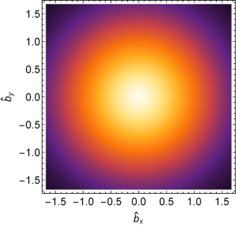
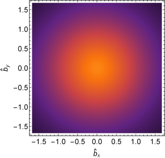
C    $0^{+}$&$1^{+}\!,d$		D    $0^{+}$&$1^{+}\!,u$

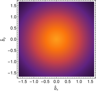
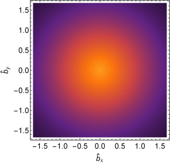
Figure 17: Transverse density profiles, Eq. (48), calculated in Ref. Chen and Roberts (2022) from flavour separated proton axial form factors. Top row: scalar-diquark-only proton. Panel A – two-dimensional plot of $\hat{\rho}_{A}^{d}(|\hat{b}|)/g_{A}^{d}$; Panel B – similar plot of $\hat{\rho}_{A}^{u}(|\hat{b}|)/g_{A}^{u}$. Removing the $1/g_{A}^{f}$ normalisation, the $b=0$ values are $\hat{\rho}_{A}^{d}(0)=-0.009$, $\rho_{A}^{u}(0)=0.097$. Bottom row: realistic proton Faddeev amplitude, including axialvector diquarks as predicted by the Faddeev equation in Fig. 8. Panel C – $\hat{\rho}_{A}^{d}(|\hat{b}|)/g_{A}^{d}$; Panel D – $\hat{\rho}_{A}^{u}(|\hat{b}|)/g_{A}^{u}$. Removing the $1/g_{A}^{f}$ normalisation, the $b=0$ values of these profiles are $\hat{\rho}_{A}^{d}(0)=-0.038$, $\hat{\rho}_{A}^{u}(0)=0.12$. N.B. $\int d^{2}\hat{b}\,\hat{\rho}_{A}^{f}(|\hat{b}|)/g_{A}^{f}=1$, $f=u,d$.

Furthermore, with flavour-separated form factors in-hand on such a large $Q^{2}$-domain, Ref. Chen and Roberts (2022) was able to calculate and contrast the $u$- and $d$-quark contributions to the associated light-front transverse spatial density profiles:

$$\hat{\rho}_{A}^{f}(|\hat{b}|)=\int\frac{d^{2}\vec{q}_{\perp}}{(2\pi)^{2}}\,{\rm e}^{i\vec{q}_{\perp}\cdot\hat{b}}G_{A}^{f}(x)\,,$$ (48)

with $G_{A}^{f}(x)$ interpreted in a frame defined by $Q^{2}=m_{N}^{2}q_{\perp}^{2}$, $m_{N}q_{\perp}=(\vec{q}_{\perp 1},\vec{q}_{\perp 2},0,0)=(Q_{1},Q_{2},0,0)$. These profiles are depicted in Fig. 17. We note that $|\hat{b}|$ and $\hat{\rho}_{A}^{f}$ are dimensionless; so, the images drawn in Fig. 17 can be mapped into physical units using:

$$\rho_{A}^{f}(|b|=|\hat{b}|/m_{N})=m_{N}^{2}\,\hat{\rho}_{A}^{f}(|\hat{b}|)\,,$$ (49)

in which case $|\hat{b}|=1$ corresponds to $|b|\approx 0.2\,$fm and $\hat{\rho}_{1}^{f}=0.1\Rightarrow\rho_{1}^{f}\approx 2.3/{\rm fm}^{2}$.

The top row of Fig. 17 provides two-dimensional renderings of the flavour-separated transverse density profiles calculated from a proton wave function which does not include axialvector diquarks, i.e., a scalar-diquark-only proton. In this case, the $u$ quark profile is far more diffuse than that of the $d$ quark, viz., its extent in the light-front transverse spatial plane is much greater. One may quantify this by reporting the associated radii: $r_{A^{d}}^{\perp}=0.24\,$fm, $r_{A^{u}}^{\perp}=0.48\,$fm, so the $d/u$ ratio of radii is $\approx 0.5$.

The bottom row of Fig. 17 was obtained using a realistic proton wave function, in which both scalar and axialvector diquarks are present with the strength determined by the Faddeev equation in Fig. 8. In this realistic case, the $d$ quark profile is not very different from that of the $u$ quark: relative to the $u$-quark profile, the intensity peak is only somewhat broader for the $d$ quark; and comparing radii,

$$r_{A^{d}}^{\perp}=0.43\,{\rm fm},\quad r_{A^{u}}^{\perp}=0.49\,{\rm fm},\quad r_{A^{d}}^{\perp}/r_{A^{u}}^{\perp}\approx 0.9\,.$$ (50)

The CSM predictions for nucleon axial and pseudoscalar form factors discussed in this section complement those for the large $Q^{2}$ behaviour of nucleon electromagnetic elastic and transition form factors reported, e.g., in Refs. Cui et al. (2020); Chen et al. (2019). One may now anticipate that predictions for form factors characterising weak interaction induced $N\to\Delta(1232)$ and $N\to N^{\ast}(1535)$ transitions will soon become available. Each will shed new light on nucleon structure; and the former, calculated on a domain that stretches from low-to-large $Q^{2}$, will likely prove valuable in developing a more reliable understanding of neutrino scattering from nucleons and nuclei.

10 Transition Form Factors of Heavy+Light Mesons

Heavy mesons ($B_{q=c,s,u}$, $D_{s}$, $D$) are special for many reasons; and their mass budgets and role in exposing constructive interference between Nature’s two known sources of mass are of particular interest herein. Consider, therefore, Fig. 18 and contrast the images with those in Fig. 1. Evidently, for heavy meson masses: (i) the HB component is largest in each case and its relative size grows as the current-masses of the valence constituents increase; (ii) all receive a significant EHM+HB interference component, but its relative strength diminishes with increasing current-masses; and (iii) for vector heavy mesons, but not pseudoscalar mesons, there is an EHM component, but its relative strength drops as the HB component grows.

A	B

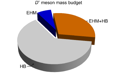
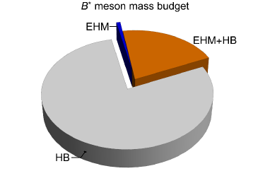
C	D

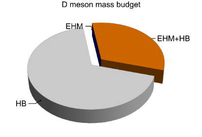
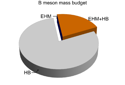
Figure 18: Mass budgets: A – $D^{\ast}$ meson; B – $B^{\ast}$-meson; C – $D$ meson; and D – $B$ meson. Each is drawn using a Poincaré invariant decomposition and the numerical values listed in Table 1. (Separation at $\zeta=2\,GeV$, calculated using information from Refs. Roberts et al. (2021); Workman et al. (2022).)

Next consider semileptonic weak-interaction transitions between heavy and light mesons. Comparing Figs. 18 and 1, it is apparent that heavy-pseudoscalar to light-pseudoscalar transitions serve to probe the relative impacts of the strength of EHM+HB interference in the initial and final states, whereas heavy-pseudoscalar to light-vector transitions overlap systems in which HB mass is dominant with those whose mass owes almost entirely to EHM. Both classes of transitions, therefore, present excellent opportunities for exposing the influence of Nature’s two known sources of mass on physical observables. These cases are of special interest, of course, because the transitions have long been used to place constraints on the values of the elements of the Cabibbo-Kobayashi-Maskawa (CKM) matrix, which parametrises quark flavour mixing in the SM.

A unifying analysis of both classes of transitions was recently completed using the SCI Xu et al. (2021); Xing et al. (2022), yielding results that compare favourably with other reliable experimental or independent theory analyses. The SCI branching fraction predictions should therefore be a reasonable guide. This is important because predictions were made for several branching fraction ratios – $R_{D_{(s)}^{(\ast)}}$, $R_{J/\psi}$, $R_{\eta_{c}}$ – whose values are direct tests of lepton universality in weak interactions: the SCI values confirm SM predictions, hence, speak for universality, as we discuss below. The analyses also used $B_{(s)}\to D_{(s)}^{\ast}$ transitions to predict the precursor functions which evolve into the universal Isgur-Wise function Isgur and Wise (1990), obtaining results in agreement with empirical inferences – Refs. (Amhis et al., 2021, Eqs. (177), (181)), (Glattauer et al., 2016, Belle).

The SCI’s successes in these applications highlight the need for kindred studies using an interaction with a closer connection to QCD. The impediment has always been the large disparity in masses that typically exists between initial and final states. That mass imbalance requires, inter alia, that any approach to the problem be simultaneously able to deal with both chiral and heavy-quark limits in quantum field theory. To date, compared with the SCI, no framework with a better link to QCD can directly surmount this difficulty. Nevertheless, following Ref. Yao et al. (2020), practicable and effective algorithms for continuum studies do now exist. They exploit the strengths of the statistical SPM as a tool for interpolating data (broadly defined) and therefrom delivering extrapolations with a rigorously defined and calculable uncertainty Cui et al. (2022). Namely, results are calculated on domains of current-quark mass for which transition form factors may straightforwardly be obtained. The SPM is then used to extrapolate those results and arrive at predictions for the physical processes of interest.

At present, CSM RL truncation predictions are available for the following transitions Yao et al. (2021, 2022): $B_{c}\to J/\psi,\eta_{c}$; $B_{(s)}\to\pi(K)$; $D_{s}\to K$; $D\to\pi,K$; and $K\to\pi$. The last process is something of a test for the approach because such $K_{\ell 3}$ transitions have long been of experimental and theoretical interest (Workman et al., 2022, Sec. 62). The calculated branching fractions are gathered in Table 4, from which it will be seen that CSMs deliver sound results.

Table 4: CSM predictions for pseudoscalar meson semileptonic branching fractions Yao et al. (2021, 2022) – each such fraction is to be multiplied by $10^{-3}$. The column labelled “ratio” is the ratio of the preceding two entries in the row, so no factor of $10^{-3}$ is applied in this column. (A $1\sigma$ SPM uncertainty is listed for the CSM predictions.) Ref. (Workman et al., 2022, PDG) lists the following values for the CKM matrix elements: $|V_{us}|=0.2245(8)$, $|V_{cd}|=0.221(4)$, $|V_{cs}|=0.987(11)$ $|V_{ub}|=0.00382(24)$; and the following lifetimes (in seconds): $\tau_{K^{+}}=1.2379(21)\times 10^{-8}$, $\tau_{D^{0}}=4.10\times 10^{-13}$, $\tau_{D_{s}^{\pm}}=5.04\times 10^{-13}$, $\tau_{\bar{B}^{0}}=1.519\times 10^{-12}$, $\tau_{\bar{B}_{s}^{0}}=1.515\times 10^{-12}$, $\tau_{B_{c}^{\pm}}=0.51\times 10^{-12}$.

${\mathpzc B}_{I\to F(\ell\nu_{\ell})}$	Refs. Yao et al. (2021, 2022)			PDG Workman et al. (2022) or other, if indicated
	$e^{+}\nu_{e}\$[51]	$\mu^{+}\nu_{\mu}\$	ratio	$e^{+}\nu_{e}\$	$\mu^{+}\nu_{\mu}\$	ratio
$K^{+}\to\pi^{0}\$	$50.0(9)\phantom{00}\$	$33.0(6)\phantom{00}\$	$0.665\phantom{(70)}\$	$50.7(6)\phantom{00}\$[51]	$33.5(3)\phantom{22}\$	$0.661(07)\$
$D^{0}\to\pi^{-}\$	$\phantom{1}2.70(12)\$	$\phantom{2}2.66(12)\$	$0.987(02)\$	$\phantom{0}2.91(4)\phantom{1}\$[51]	$\phantom{0}2.67(12)\$	$0.918(40)\$
$D_{s}^{+}\to K^{0}\$	$\phantom{1}2.73(12)\$	$\phantom{2}2.68(12)\$	$0.982(01)\$	$\phantom{00}3.25(36)\$Ablikim et al. (2019)
$D^{0}\to K^{-}\$	$39.0(1.7)\$	$38.1(1.7)\$	$0.977(01)\$	$\phantom{0}35.41(34)\phantom{1}\$[51]	$34.1(4)\phantom{22}\$	$0.963(10)\$
	$\mu^{-}\bar{\nu}_{\mu}\$[51]	$\tau^{-}\bar{\nu}_{\tau}\$	ratio	$\mu^{-}\bar{\nu}_{\mu}\$	$\tau^{-}\bar{\nu}_{\tau}\$	ratio
$\bar{B}^{0}\to\pi^{+}\$	$\phantom{11}0.162(44)\$	$\phantom{11}0.120(35)\$	$0.733(02)\$	$\phantom{01}0.150(06)\$[51]
$\bar{B}_{s}^{0}\to K^{+}\$	$\phantom{11}0.186(53)\$	$\phantom{11}0.125(37)\$	$0.667(09)\$
$B_{c}\to\eta_{c}\$	$\phantom{00}8.10\,(45)\phantom{0}\$	$\phantom{00}2.54(10)\phantom{0}\$	$0.31(2)\phantom{00}\$
$B_{c}\to J/\psi\$	$\phantom{0}17.2\,(1.9)\phantom{0}\$	$\phantom{0}4.17(66)\$	$0.24(5)\phantom{00}\$

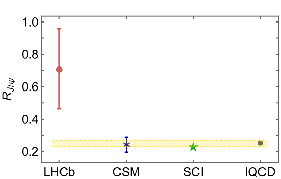
Figure 19: Ratio $R_{J/\psi}$ in Eq. (51) – red circle, empirical result (Aaij et al., 2018, LHCb); blue asterisk – CSM prediction Yao et al. (2021); green star – SCI prediction Xing et al. (2022); grey circle – lQCD result Harrison et al. (2020a, b); and gold band – unweighted mean of central values from several calculations Tran et al. (2018); Issadykov and Ivanov (2018); Wang and Zhu (2019); Leljak et al. (2019); Hu et al. (2020); Zhou et al. (2020).

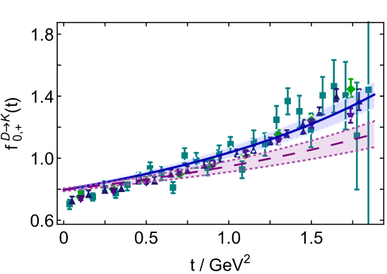
Figure 20: $D\to K$ transition form factors. $f_{+}$ – solid blue curve; $f_{0}$ – long-dashed purple curve; and like-coloured shaded bands – associated SPM uncertainty in each case. Data: cyan squares Widhalm et al. (2006); green diamonds Besson et al. (2009); dark-blue up-triangles Ablikim et al. (2015); and indigo down-triangles Ablikim et al. (2017).

One of the key results in Ref. Yao et al. (2021) concerns a ratio of $B_{c}^{+}\to J/\psi$ branching fractions measured for the first time by the LHCb Collaboration fairly recently Aaij et al. (2018):

$$R_{J/\psi}:=\frac{{\mathpzc B}_{B_{c}^{+}\to J/\psi\tau\nu}}{{\mathpzc B}_{B_{c}^{+}\to J/\psi\mu\nu}}=0.71\pm 0.17\,{\rm(stat)}\pm 0.18\,{\rm(syst)}\,.$$ (51)

This value is plotted in Fig. 19 and compared with the CSM prediction and other Standard Model calculations. Evidently, the LHCb measurement lies approximately $2\sigma$ above the values predicted by reliable SM calculations. If future, precision experiments do not deliver a markedly lower central value, then one might begin to judge that lepton flavour universality is violated in $B_{c}\to J/\psi$ semileptonic decays. As yet, however, the experimental precision is insufficient to support such a claim. Furthermore, a compelling case would need to include information on $B_{c}\to\eta_{c}$ semileptonic decays. The CSM prediction is $R_{\eta_{c}}=0.313(22)$ – see Table 4; the SCI result is $R_{\eta_{c}}=0.25$ Xu et al. (2021); and a mean value of $0.31(4)$ is obtained from modern continuum analyses Tran et al. (2018); Issadykov and Ivanov (2018); Wang and Zhu (2019); Leljak et al. (2019); Hu et al. (2020); Zhou et al. (2020). An experimental value is lacking.

The array of analyses in Ref. Yao et al. (2022) yield novel results in other areas. Of particular interest are the discussions of $D^{0}\to K^{-}$ transition form factors and the value of $|V_{cs}|$. Two independent form factors characterise $0^{+}\to 0^{+}$ transitions, viz. vector and scalar, $f_{+,0}(t)$, respectively, where $t$ is the Mandelstam variable whose value expresses the momentum transferred to the final state. The CSM predictions are plotted in Fig. 20 and compared with available data Widhalm et al. (2006); Besson et al. (2009); Ablikim et al. (2015, 2017). The CSM result is largely consistent with this collection, although there may be a hint that it is too high at lower $t$ values. Concerning branching fractions, form factor contributions from this domain are important. It is therefore notable that, within mutual uncertainties, the CSM value for $f_{+}^{D\to K}(0)=0.796(9)$ agrees with the $N_{f}=2+1+1$ lQCD result in Ref. Lubicz et al. (2017): $0.765(31)$.

With the form factors in Fig. 20, Ref. Yao et al. (2022) obtained the $D^{0}\to K^{-}$ branching fractions listed in Table 4 when using the value of $|V_{cs}|$ listed in the caption: evidently, both the $e^{+}\nu_{e}$ and $\mu^{+}\nu_{\mu}$ fractions exceed their respective PDG values. On the other hand, the ratio agrees within $1.4\sigma$; so, a common overall factor can remedy the mismatch. Adopting this perspective, then the value $|V_{cs}|=0.937(17)$ combined with the CSM form factors delivers branching fractions that match the PDG values, viz. $3.52(18)$% and $3.44(18)$%, respectively. Actually, referring to Ref. (Workman et al., 2022, Sec. 12.2.4), one sees that the inferred CSM value is both commensurate with and more precise than one of the two used to arrive at the PDG average listed in the caption of Table 4. With $|V_{cs}|=0.937(17)$ used instead to compute this average, one finds a slightly more precise central value that is $1\sigma$ lower:

$$|V_{cs}|=0.974(10)\,.$$ (52)

A		B

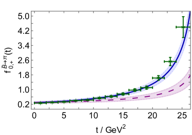
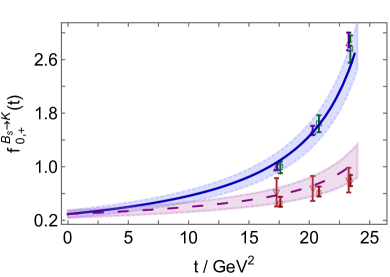
Figure 21: CSM predictions for $B_{(s)}$ semileptonic transition form factors: $f_{+}$ – solid blue curve; $f_{0}$ – long-dashed purple curve; and SPM uncertainty in each – like-coloured shaded bands. Left panel – A. $\bar{B}^{0}\to\pi^{+}$. Data (green stars): reconstructed from the average (Amhis et al., 2021, Tab. 81) of data reported in Refs. del Amo Sanchez et al. (2011); Ha et al. (2011); Lees et al. (2012); Sibidanov et al. (2013). Right panel – B. $\bar{B}_{s}^{0}\to K^{+}$. lQCD results: $f_{+}$ – indigo open up-triangles Bouchard et al. (2014) and green open boxes Flynn et al. (2015); $f_{0}$ — brown open down-triangles Bouchard et al. (2014) and red open circles Flynn et al. (2015).

Predictions for semileptonic $\bar{B}^{0}\to\pi^{+}$, $\bar{B}_{s}^{0}\to K^{+}$ transition form factors and branching fractions were also delivered in Ref. Yao et al. (2022). As emphasised above, such processes present challenges because $\pi$, $K$ are Nambu-Goldstone bosons and there is a huge disparity between the masses of the initial and final states. Consequently, comparisons with data serve as a stringent test of the new CSM algorithms.

CSM predictions for the $\bar{B}^{0}\to\pi^{+}$ transition form factors are depicted in Fig. 21A. Regarding $f_{+}^{\bar{B}\to\pi}$, data have been collected by two collaborations del Amo Sanchez et al. (2011); Ha et al. (2011); Lees et al. (2012); Sibidanov et al. (2013): within mutual uncertainties, the CSM predictions agree with this data. The data support a value

$$f_{+}^{\bar{B}\to\pi}(t=0)=0.27(2)\,,$$ (53)

which is consistent with the CSM prediction Yao et al. (2022): $0.29(5)$.

Using the form factors in Fig. 21A, one obtains the $\bar{B}^{0}\to\pi^{+}$ branching fractions in Table 4. The PDG lists a result for the $\mu^{-}\nu_{\mu}$ final state, which matches the CSM prediction within mutual uncertainties. Precise agreement is obtained using

$$|V_{ub}|=0.00374(44)\,.$$ (54)

This value is commensurate with other analyses of ${\mathpzc B}_{\bar{B}^{0}\to\pi^{+}\mu^{-}\bar{\nu}_{\mu}}$ (Workman et al., 2022, Sec. 76.3) and thus increases tension with the higher value inferred from inclusive decays. No data is available on the $\tau^{-}\nu_{\tau}$ final state; so, the $\tau$:$\mu$ ratio is empirically unknown. Here, a $N_{f}=2+1$-flavour lQCD study yields $0.69(19)$ Flynn et al. (2015), which, within its uncertainty, matches the CSM result: $0.733(2)$.

Fig. 21B displays CSM predictions for the $\bar{B}_{s}\to K^{+}$ form factors. Although the $B_{s}\to K^{-}$ transition was recently observed Aaij et al. (2021), with the measurement yielding the branching fraction

$${\mathpzc B}_{B_{s}^{0}\to K^{-}\mu^{+}\nu_{\mu}}=[0.106\pm 0.005_{\rm stat}\pm 0.008_{\rm syst}]\times 10^{-3}\,,$$ (55)

no form factor data are yet available. Comparisons are therefore made in Fig. 21B with results obtained using $N_{f}=2+1$-flavour lQCD Bouchard et al. (2014); Flynn et al. (2015). Owing to difficulties encountered when using lattice methods to calculate form factors of heavy+light mesons, lQCD results are limited to a few points on the domain $t\gtrsim 17\,$GeV² – see Fig. 21B. Today, lattice analyses typically employ such results to construct a least-squares fit to the form factor points, using some practitioner-favoured functional form. That fit is then employed to define the form factor on the whole kinematically accessible domain: $0\lesssim t\lesssim 25\,$GeV² in this case. It is worth noting that at this time, given the small number of points and their limited precision, the SPM cannot gainfully be used to develop function-form unbiased interpolations and extrapolations of the lQCD output.

The CSM form factors in Fig. 21B yield the $\bar{B}_{s}^{0}\to K^{+}$ branching fractions in Table 4. Fig. 22A compares the $\mu^{-}\bar{\nu}_{\mu}$ value with the measurement in Eq. (55) and also results obtained via various other means. Experiment and theory only agree because the theory uncertainty is large. The unweighted theory average is $0.141(44)$‰ and the uncertainty weighted mean is $0.139(08)$‰. These values increase when entries V–VI Flynn et al. (2015); Bazavov et al. (2019) are omitted: unweighted $0.159(38)$‰ and uncertainty weighted $0.156(10)$‰. The extrapolations employed in V–VI Flynn et al. (2015); Bazavov et al. (2019) lead to values of $f_{+}^{\bar{B}_{s}\to K}(0)$ that are $\sim 50$% of those obtained in I–IV Wu et al. (2006); Faustov and Galkin (2013); Xiao et al. (2014); Bouchard et al. (2014): $0.148(53)$ vs. $0.299(86)$. This can explain the difference in branching fractions: V–VI vs. I–IV in Fig. 22A. Significantly, a different approach to fitting and extrapolating lQCD results, using the LHCb datum, Eq. (55), as an additional constraint, produces Gonzàlez-Solís et al. (2021): $f_{+}^{\bar{B}_{s}\to K}(0)=0.211(3)$.

Ref. Gonzàlez-Solís et al. (2021) also infers $f_{+}^{\bar{B}\to\pi}(0)=0.255(5)$, leading to $f_{+}^{\bar{B}_{s}\to K}(0)/f_{+}^{\bar{B}\to\pi}(0)<1$. This outcome conflicts with the CSM prediction, which has $f_{+}^{\bar{B}_{s}\to K}(0)/f_{+}^{\bar{B}\to\pi}(0)>1$ at the 85% confidence level (Yao et al., 2022, Eq. (9)), and the results in a raft of other studies, e.g., Refs. Melikhov (2002); Faessler et al. (2002); Ebert et al. (2003); Ball and Zwicky (2005); Wu et al. (2006); Khodjamirian et al. (2007); Lü et al. (2007); Ivanov et al. (2007); Faustov and Galkin (2013). It is probable, therefore, that the Ref. Gonzàlez-Solís et al. (2021) value for $f_{+}^{\bar{B}_{s}\to K}(0)$ is too small. It is worth remarking that the SCI is unclear on the value of this ratio. It produces $f_{+}^{\bar{B}_{s}\to K}(0)/f_{+}^{\bar{B}\to\pi}(0)<1$, but the individual $t=0$ values are too large by a factor of two (Xu et al., 2021, Table 3A). On the other hand, the $t=0$ value of the kindred ratio of vector form factors in $\bar{B}_{s}\to K^{\ast}$, $\bar{B}\to\rho$ transitions is greater than unity (Xing et al., 2022, Table 1A). Notably, the ratio $f_{+}^{\bar{B}_{s}\to K}(0)/f_{+}^{\bar{B}\to\pi}(0)$ is a marker for SU$(3)$-flavour symmetry breaking and its modulation by EHM; so it is worth reaching a sound conclusion on the value of the ratio. It is here relevant to observe that $f_{K}/f_{\pi}=1.2>1$.

A		B

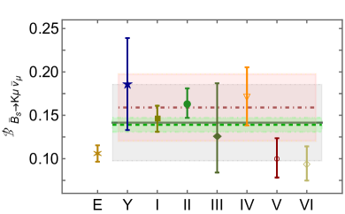
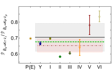
Figure 22: Left panel – A. Branching fraction ${\mathpzc B}_{\bar{B}_{s}^{0}\to K^{+}\mu^{-}\bar{\nu}_{\mu}}$ computed in Ref. Yao et al. (2022), “Y”, compared with the value in Eq. (55), “E”, viz. a measurement of ${\mathpzc B}_{B_{s}^{0}\to K^{-}\mu^{+}\nu_{\mu}}$ Aaij et al. (2021) and some results obtained using other approaches: continuum I – III Wu et al. (2006); Faustov and Galkin (2013); Xiao et al. (2014); and lattice IV – VI Bouchard et al. (2014); Flynn et al. (2015); Bazavov et al. (2019). Right panel – B. Branching fraction ratio ${\mathpzc B}_{\bar{B}_{s}^{0}\to K^{+}\tau^{-}\bar{\nu}_{\tau}}/{\mathpzc B}_{\bar{B}_{s}^{0}\to K^{+}\mu^{-}\bar{\nu}_{\mu}}$ computed in Ref. Yao et al. (2022) compared with some results obtained using other approaches. Legend matches Panel A, except “P(E)” is the result from Gonzàlez-Solís et al. (2021), i.e., an estimate constrained by the datum in Ref. Aaij et al. (2021). Both panels – Grey line: unweighted mean of theory results. Pink dot-dashed line: unweighted mean of theory results, omitting V–VI. Green dashed line: uncertainty-weighted average of theory results. Like-coloured bands mark associated uncertainties in each case.

Regarding the $\tau\nu_{\tau}$ final state in $\bar{B}_{s}\to K$ transitions, no empirical information is currently available; hence, none on the $|V_{ub}|$-independent ratio which would test lepton flavour universality. In Fig. 22B, therefore, we compare the CSM prediction for this ratio, drawn from Table 4, with results obtained via other means. The unweighted average of theory results is $0.705(87)$ and the uncertainty weighted mean is $0.678(03)$. Omitting entries V–VI Flynn et al. (2015); Bazavov et al. (2019), these values are: unweighted $0.653(41)$ and uncertainty weighted $0.677(03)$. Within sound analyses, many uncertainties cancel in this ratio; so the results should be more reliable than any calculation of either fraction alone. Nevertheless, the values are widely scattered, indicating that there is ample room for improving the precision of $\bar{B}_{s}^{0}\to K$ theory. Of course, measurements enabling extraction of $B_{s}^{0}\to K^{-}$ form factors would be very useful, too, for refining both (a) comparisons with theory and between theory analyses and (b) making progress toward a more accurate value of $|V_{ub}|$.

Such predictions for heavy-to-light meson electroweak transition form factors are a new branch of application for CSMs. They are far more sophisticated and robust than the Schwinger-function parametrisation-based analyses in, e.g., Refs. Ivanov et al. (1999, 2007); El-Bennich et al. (2011) and significantly improve upon earlier RL truncation studies of $\pi_{\ell 3}$ and $K_{\ell 3}$ transitions Ji and Maris (2001); Chen et al. (2013). The keys to these advances are an improved understanding of RL truncation and the capacity to greatly expand its quark mass and mass-splitting domains of applicability using the SPM. Fairly soon, one can expect these advances to be exploited in the study of kindred baryon transitions.

11 Distribution Functions

Hadron parton DFs are probability densities: each one describes the light-front fraction, $x$, of the hadron’s total momentum carried by a given parton species within the bound-state Holt and Roberts (2010). They are a much prized source of hadron structure information; and following the quark discovery experiments fifty years ago Taylor (1991); Kendall (1991); Friedman (1991); Friedman et al. (1991), measurements interpretable in terms of hadron DFs have been awarded a high priority. For much of this time, DFs were inferred from global fits to data, with the results viewed as benchmarks. Such fitting remains crucial, providing input for the conduct of a huge number of experiments worldwide; but the past decade has seen the dawn of a new theory era. Continuum and lattice studies of QCD are beginning to yield robust predictions for the pointwise behaviour of DFs; and these developments are exposing potential conflicts with the fitting results Roberts et al. (2021); Chang and Roberts (2021); Cui et al. (2022a, b); Chang et al. (2022); Lu et al. (2022); de Paula et al. (2022).

Notwithstanding the enormous expense of time and effort, much yet remains to be learnt before proton and pion structure may be judged as understood in terms of DFs. For instance and most simply, it is still unclear whether there are differences between the distributions of partons within the proton (Nature’s most fundamental bound-state) and the pion (Nature’s most fundamental (near) Nambu-Goldstone boson). Plainly, if there are differences, then they must be explained. As we have stressed above, answering the question of similarity/difference between proton and pion DFs is particularly important today as science seeks to expose and explain EHM Roberts and Schmidt (2020); Roberts (2020, 2021); Roberts et al. (2021); Binosi (2022); Papavassiliou (2022).

Regarding DFs measured in processes that do not resolve beam or target polarisation, practitioners experienced and involved with solving bound-state problems in QCD have learnt that, at the hadron scale, $\zeta_{\cal H}<m_{p}$, valence-quark DFs in the proton and pion behave as follows Brodsky et al. (1995); Yuan (2004); Cui et al. (2022a, b); Chang et al. (2022):

$${\mathpzc d}^{p}(x;\zeta_{\cal H}),{\mathpzc u}^{p}(x;\zeta_{\cal H})\stackrel{{\scriptstyle x\simeq 1}}{{\propto}}(1-x)^{3}\,,\quad\bar{\mathpzc d}^{\pi}(x;\zeta_{\cal H}),{\mathpzc u}^{\pi}(x;\zeta_{\cal H})\stackrel{{\scriptstyle x\simeq 1}}{{\propto}}(1-x)^{2}\,;$$ (56)

and it subsequently follows from the DGLAP equations Dokshitzer (1977); Gribov and Lipatov (1971); Lipatov (1975); Altarelli and Parisi (1977) that the large-$x$ power on the related gluon DF is approximately one unit larger; and that for sea quark DFs is roughly two units larger. Moreover, as the resolving scale increases to $\zeta>\zeta_{\cal H}$, all these exponents grow logarithmically. However, fueling controversy and leading some to question the veracity of QCD Aicher et al. (2010); Cui et al. (2022a, b), these constraints are typically ignored in fits to the world’s data on deep inelastic scattering (DIS) and kindred processes Ball et al. (2016); Hou et al. (2021); Bailey et al. (2021); Novikov et al. (2020); Barry et al. (2021). Furthermore, largely because pion data are scarce (Roberts et al., 2021, Table 9.5), proton and pion data have never been considered simultaneously. Therefore, the unified body of results in Ref. Lu et al. (2022), which uses a single symmetry-preserving framework to predict the pointwise behaviour of all proton and pion DFs – valence, glue, and four-flavour-separated sea – is a significant advance.

In order to sketch this progress, it is necessary to recall that the modern approach to the CSM prediction of hadron DFs is based on a single proposition Raya et al. (2022); Cui et al. (2022a, b); Chang et al. (2022); Lu et al. (2022):

P1

… There is an effective charge, $\alpha_{1\ell}(k^{2})$, which, when used to integrate the one-loop perturbative-QCD DGLAP equations, defines a DF evolution scheme that is all-orders exact.

As noted in connection with Fig. 3, charges of this sort are discussed in Refs. Grunberg (1984, 1989); Dokshitzer (1998). They need not be process-independent (PI); hence, not unique. Moreover, the results delivered are independent of the explicit form of $\alpha_{1\ell}(k^{2})$. Notwithstanding these things, a suitable PI charge is available, viz. the coupling discussed in Sec. 4, which has proved efficacious. In being defined by an observable – in this instance, structure functions – each such $\alpha_{1\ell}(k^{2})$ is Deur et al. (2016): consistent with the renormalisation group and renormalisation scheme independent; everywhere analytic and finite; and, crucially, provides an infrared completion of any standard perturbative running coupling.

P1 was used in Refs. Cui et al. (2021, 2020); Raya et al. (2022); Han et al. (2021); de Paula et al. (2022) to deliver meson DFs with a flavour symmetric sea. A generalisation, which expresses key quark current-mass effects in the evolution kernels, was introduced in Ref. Lu et al. (2022) and used for the proton and pion. It features a threshold function ${\cal P}_{qg}^{\zeta}\sim\theta(\zeta-\delta_{\mathpzc f})$, which ensures that a given quark flavour only becomes active in DF evolution when the energy scale exceeds a value determined by the quark’s mass (Roberts et al., 2021, Fig. 2.5): $\delta_{u,d}\approx 0$, $\delta_{s}\approx 0.1\,$GeV, $\delta_{c}\approx 0.9\,$GeV. The impact of this modification is readily anticipated. Supposing that all quark flavours are light, then each would be emitted with equal probability on $\zeta>\zeta_{\cal H}$; so, evolution would produce a certain gluon momentum fraction in the hadron plus a sea-quark fraction shared equally between all quark flavours. Considering mass differences between the quarks, with some flavours being heavier than the light-quark threshold, then evolution on $\zeta>\zeta_{\cal H}$ will generate a gluon momentum fraction that is practically unchanged from the all-light quark case and a sea-quark fraction divided amongst the quarks in roughly inverse proportion to their mass.

It is worth reiterating here that $\zeta_{\cal H}$ is the scale at which the valence quasiparticle degrees-of-freedom carry all properties of a given hadron Ding et al. (2020a, b); Cui et al. (2021, 2020); Han et al. (2021); Chang and Roberts (2021); Xie et al. (2022); Raya et al. (2022); Cui et al. (2022a, b); Chang et al. (2022); Lu et al. (2022); de Paula et al. (2022). Moreover, the value of this scale is a prediction. Using the PI charge discussed in Sec. 4 to construct bound-state kernels informed by Refs. Qin et al. (2011); Binosi et al. (2015), then

$$\zeta_{\cal H}=0.331(2)\,{\rm GeV}.$$ (57)

The value in Eq. (57) is the same for all hadrons.

Furthermore, combined with evolution according to P1, the character of $\zeta_{\cal H}$ ensures that all hadron DFs are intertwined at every scale $\zeta$. Hence, this perspective suggests that it is incorrect to choose independent, uncorrelated functions to parametrise the DFs of different parton species when fitting data at any scale $\zeta>\zeta_{\cal H}$. If one nevertheless chooses to ignore the innate associations, then DFs with unphysical features may be obtained – see, e.g., Ref. (Cui et al., 2022a, Fig. 6).

A		B

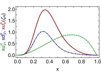
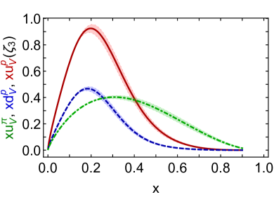
Figure 23: Left panel – A. Proton and pion hadron scale valence parton DFs: $x{\mathpzc u}^{p}(x;\zeta_{\cal H})$ – solid red curve; $x{\mathpzc d}^{p}(x;\zeta_{\cal H})$ – dot-dashed blue curve; and $x{\mathpzc u}^{\pi}(x;\zeta_{\cal H})$ – dashed green curve. Right panel – B. Valence DFs in panel A evolved to $\zeta_{3}=m_{J/\psi}=3.097\,$GeV according to P1. The band surrounding each CSM curve expresses the response to a $\pm 5$% variation in $\zeta_{\cal H}$.

CSM predictions for the $\zeta=\zeta_{\cal H}$ proton and pion valence DFs are drawn in Fig. 23A. The following points are significant. (i) Each DF is consistent with the relevant large-$x$ scaling law in Eq. (56). Hence, from the outset, whilst the $\zeta=\zeta_{\cal H}$ momentum sum rules for each hadron are necessarily saturated by valence degrees-of-freedom, viz.

$$\langle x\rangle_{{\mathpzc u}_{p}}^{\zeta_{\cal H}}=0.687\,,\;\langle x\rangle_{{\mathpzc d}_{p}}^{\zeta_{\cal H}}=0.313\,,\;\langle x\rangle_{{\mathpzc u}_{\pi}}^{\zeta_{\cal H}}=0.5\,,$$ (58)

the proton and pion valence DFs nevertheless have markedly different $x$-dependence. (Nature’s approximate ${\cal G}$-parity symmetry Lee and Yang (1956) entails $\bar{\mathpzc d}_{\pi}(x;\zeta)={\mathpzc u}_{\pi}(x;\zeta)$.) (ii) Owing to DCSB Lane (1974); Politzer (1976); Pagels (1979); Pagels and Stokar (1979); Higashijima (1984); Roberts and Schmidt (2000); Binosi et al. (2017), an important corollary of EHM, QCD dynamics simultaneously produce a dressed light-quark mass function, $M_{u,d}(k^{2})$, that is large at infrared momenta, $M_{D}:=M_{u,d}(k^{2}\simeq 0)\approx 0.4\,$GeV and an almost massless pion, $m_{\pi}^{2}/M^{2}_{D}\approx 0.1$ – see Ref. (Roberts et al., 2021, Sec. 2). As a result, ${\mathpzc u}^{\pi}(x;\zeta_{H})$ is Nature’s most dilated hadron-scale valence DF. This is highlighted by Fig. 23A and Refs. Cui:2021dlm; Cui et al. (2020), and implicit in numerous other symmetry-preserving analyses, e.g., Refs. Gao et al. (2014); Binosi et al. (2019); Ding et al. (2019); Lu et al. (2021).

Evolving the DFs in Fig. 23A according to P1, one obtains the $\zeta=m_{J/\psi}=:\zeta_{3}$ distributions in Fig. 23B. Plainly, although the profiles change, the relative dilation of the DFs is preserved and is therefore a verifiable prediction of the EHM paradigm.

Given that Fig. 23B depicts the first CSM predictions for proton valence-quark DFs, one might question their reliability. That issue can partly be addressed through a comparison with lQCD results. The calculation of individual valence DFs using lQCD is problematic owing to difficulties in handling so-called disconnected contributions Alexandrou et al. (2013). In the continuum limit, however, disconnected diagrams do not contribute to the isovector DF $[{\mathpzc u}^{p}(x;\zeta)-{\mathpzc d}^{p}(x;\zeta)]$, so computations of this difference are available Lin et al. (2020); Alexandrou et al. (2021). Both analyses use the quasidistribution approach Ji et al. (2021), but the lattice algorithms and configurations are somewhat different. Their comparison with CSM predictions is depicted in Fig. 24. The level of agreement is encouraging; especially because refinements of both continuum and lattice calculations may be anticipated. For instance, the CSM predictions were obtained using a simplified proton Faddeev amplitude and the lattice studies must address issues with, inter alia, the pion masses used, lattice artefacts and systematic errors, and convergence of the boost expansion in the quasidistribution approach. (The last of these is a particular hindrance to lQCD extractions of DF endpoint behaviour Xu et al. (2018).)

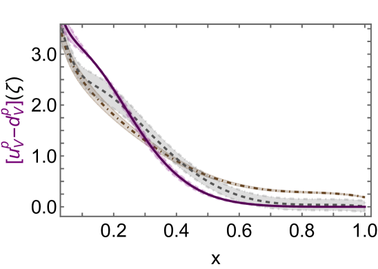
Figure 24: Isovector distribution $[{\mathpzc u}^{p}(x;\zeta)-{\mathpzc d}^{p}(x;\zeta)]$. CSM prediction – solid purple curve, $\zeta=\zeta_{3}$; lQCD result from Ref. Lin et al. (2020) – dashed grey curve, $\zeta=\zeta_{3}$; lQCD result from Ref. Alexandrou et al. (2021) – dot-dashed brown curve, $\zeta=\zeta_{2}$. Like-coloured band bracketing each curve indicates associated uncertainty.

In typical evolution kernels, gluon splitting yields quark+antiquark pairs of all flavours with equal probability. However, it was long ago argued Field and Feynman (1977) that because the proton contains two valence $u$ quarks and one valence $d$ quark, the Pauli exclusion principle should force gluon splitting to prefer $d+\bar{d}$ production over $u+\bar{u}$. Consequently, when implementing evolution of proton singlet and glue DFs, Ref. Lu et al. (2022) followed Ref. Chang et al. (2022) and introduced a small Pauli blocking factor into the gluon splitting function. This correction preserves baryon number, but shifts momentum into $d+\bar{d}$ from $u+\bar{u}$, otherwise leaving the sum of sea-quark momentum fractions unchanged. It vanishes with increasing $\zeta$, in order to express the declining influence of valence-quarks as the proton’s sea and glue content increases.

The resulting CSM predictions for $\zeta=\zeta_{3}$ proton and pion glue DFs are drawn in Fig. 25A. The glue-in-$\pi$ DF is directly related to the $\zeta=2\,{\rm GeV}=:\zeta_{2}$ result discussed in Ref. Chang and Roberts (2021), which is drawn in Fig. 25B: evidently, it agrees with a recent lQCD calculation of the glue-in-$\pi$ DF Fan and Lin (2021). Furthermore, reproducing the pattern seen with valence-quark DFs in Fig. 23, Fig. 25A reveals that the glue-in-$\pi$ DF possesses significantly more support on the valence domain, $x\gtrsim 0.1$, than the glue-in-$p$ DF. Once again, this feature is a measurable expression of EHM.

The $\zeta=\zeta_{3}$ light-quark sea DFs for the proton and pion are depicted in Fig. 25C. The EHM-induced pattern is also apparent here, viz. the sea-in-$\pi$ DF possesses greater support on $x\gtrsim 0.1$ than the kindred sea-in-$p$ DFs. DFs of the heavier sea quarks are also generated via evolution, with the results drawn in Fig. 25D. Interestingly, the $\zeta=\zeta_{3}$ $s$ and $c$ quark DFs are similar in size to those of the light-quark sea DFs; and, for these heavier quarks, too, the pion DFs have significantly greater support on the valence domain, $x\gtrsim 0.1$, than the related proton DFs.

A		B
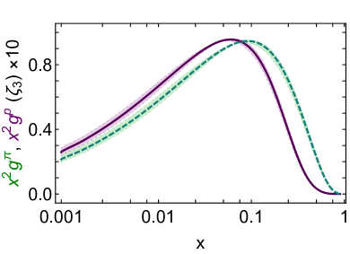
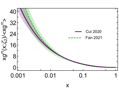
C		D

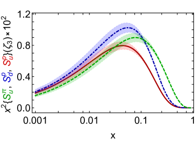
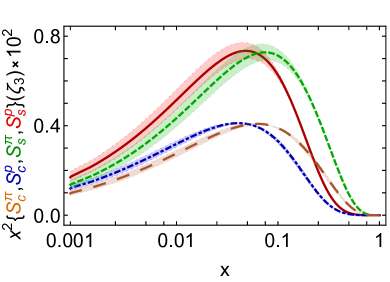
Figure 25: Left upper panel – A. Glue DFs – $x^{2}{\mathpzc g}$, in the proton (solid purple curve) and pion (dashed green curve) at $\zeta=\zeta_{3}$. Right upper panel – B. Comparison between continuum (Cui et al., 2020, Cui 2020) and lattice (Fan and Lin, 2021, Fan 2021) results for the glue-in-pion DF at $\zeta=2\,$GeV. Left lower panel – C. Proton and pion light quark sea DFs: $x^{2}{\mathpzc S}_{u}^{p}(x;\zeta_{3})$ – solid red curve; $x^{2}{\mathpzc S}_{d}^{p}(x;\zeta_{3})$ – dashed blue curve; and $x^{2}{\mathpzc S}_{u}^{\pi}(x;\zeta_{3})$ – dot-dashed green curve. Right lower panel – D. Proton and pion $c$- and $s$-quark sea DFs: $x^{2}{\mathpzc S}_{s}^{p}(x;\zeta_{3})$ – solid red curve; $x^{2}{\mathpzc S}_{s}^{\pi}(x;\zeta_{3})$ – dashed green curve; $x^{2}{\mathpzc S}_{c}^{p}(x;\zeta_{3})$ – dot-dashed blue curve; and $x^{2}{\mathpzc S}_{c}^{\pi}(x;\zeta_{3})$ – long-dashed orange curve. The band surrounding each CSM curve expresses the response to a $\pm 5$% variation in $\zeta_{\cal H}$. The uncertainty in the lQCD result is similarly indicated in Panel B.

An analysis of the endpoint exponents of all $\zeta=\zeta_{3}$ DFs is also contained in Ref. Lu et al. (2022) along with simple interpolations of each DF that can readily be used by any practitioner – Ref. (Lu et al., 2022, Table 1). It is worth reiterating the following remarks about the endpoint exponents.

(i)

The power laws express measurable effective exponents, obtained from separate linear fits to $\ln[x{\mathpzc p}(x)]$ on the domains $0<x<0.005$, $0.85<x<1$. (Here, ${\mathpzc p}(x)$ denotes a generic DF.)

(ii)

Within mutual uncertainties, proton and pion DFs have the same power-law behaviour on $x\simeq 0$:

$$\alpha^{p,\pi}_{\rm valence}\approx-0.22\,,\quad\alpha^{p,\pi}_{\rm glue}\approx-1.6\,,\quad\alpha^{p,\pi}_{\rm sea}\approx-1.5\,.$$ (59)

(iii)

On $x\simeq 1$, the following relationships exist for and between pion and proton DF exponents:

$$\beta^{\pi}_{\rm valence} \approx 2.5\,,\quad\beta^{p}_{\rm valence}\approx\beta^{\pi}_{\rm valence}+1.6\,,$$ (60a)

$$\beta^{p,\pi}_{\rm glue} \approx\beta^{p,\pi}_{\rm valence}+1.4\,,\quad\beta^{p,\pi}_{\rm sea}\approx\beta^{p,\pi}_{\rm valence}+2.4\,.$$ (60b)

(iv)

Given (ii), (iii), then the CSM predictions are consistent with the QCD expectations discussed in connection with Eq. (56).

(v)

Existing phenomenological fits to relevant scattering data typically arrive at DFs which are inconsistent with (ii), (iii); hence, fail to meet many QCD-based expectations, e.g., Refs. Accardi et al. (2016); Ball et al. (2017); Hou et al. (2021); Novikov et al. (2020); Barry et al. (2021). This point is also discussed elsewhere Courtoy and Nadolsky (2021); Cui et al. (2022a, b).

Owing to the Pauli blocking factor described above and as evident in Fig. 25C, the DFs calculated in Ref. Lu et al. (2022) express an in-proton separation between $\bar{d}$ and $\bar{u}$ distributions. This entails a violation of the Gottfried sum rule Gottfried (1967); Brock et al. (1995), which has been seen in experiments Amaudruz et al. (1991); Arneodo et al. (1994); Baldit et al. (1994); Towell et al. (2001); Dove et al. (2021). Using the proton DFs in Fig. 25C then, on the domain covered by the measurements in Refs. Amaudruz et al. (1991); Arneodo et al. (1994), one obtains

$$\int_{0.004}^{0.8}dx\,[\bar{\mathpzc d}(x;\zeta_{3})-\bar{\mathpzc u}(x;\zeta_{3})]=0.116(12)$$ (61)

for the Gottfried sum rule discrepancy. This value matches that inferred from recent fits to a large sample of high-precision data ($\zeta=2\,$GeV) (Hou et al., 2021, CT18): 0.110(80); and is far more precise.

The result in Eq. (61) corresponds to a strength for the Pauli blocking term in the gluon splitting function that shifts just $\approx 25$% of the $u$ quark sea momentum fraction into the $d$ quark sea at $\zeta=\zeta_{2}$. Changing the strength by $\pm 25$% leads to the uncertainty indicated in Eq. (61). Data from the most recent experiment focused on the asymmetry of antimatter in the proton (Dove et al., 2021, E906) are presented in Fig. 26A. They may be compared with the CSM result obtained using the proton DFs in Fig. 25C. Evidently, a modest Paul blocking effect in the gluon splitting function is sufficient to explain modern data.

A		B

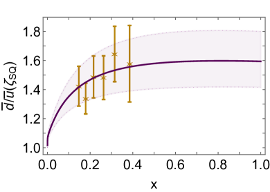
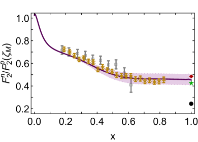
Figure 26: Left panel – A. Ratio of light antiquark DFs. Data: Ref. (Dove et al., 2021, E906). CSM result (solid purple curve) obtained from valence-quark DFs in Fig. 23 after evolution to $\zeta^{2}=\zeta_{\rm SQ}^{2}=30\,$GeV² Lu et al. (2022). The shaded band expresses the impact of a $\pm 25$% variation in the strength of Pauli blocking. Right panel – B. Neutron-to-proton structure function ratio. Data: (Tkachenko et al., 2014, BoNuS) – open grey squares; and (Abrams et al., 2022, MARATHON) – gold asterisks. Contemporary CSM result (solid purple curve) obtained from valence-quark DFs in Fig. 23 after evolution to $\zeta=\zeta_{M}=2.7\,$GeV Chang et al. (2022); Lu et al. (2022). Other predictions: green star – helicity conservation in the QCD parton model Farrar and Jackson (1975); Brodsky and Lepage (1979); Brodsky et al. (1995); red diamond – large-$x$ estimate based on Faddeev equation solutions Roberts et al. (2013); and retaining only scalar diquarks in the proton wave function, which produces a large-$x$ value for this ratio that lies in the neighbourhood of the filled circle Close and Thomas (1988); Xu et al. (2015). The band surrounding the CSM curve expresses the response to a $\pm 5$% variation in the size of axialvector diquark contributions to the proton charge. It is only noticeable on the valence quark domain.

Proton and, in principle, neutron structure functions – $F_{2}^{p,n}$ – can be measured in the DIS of electrons from nucleons Taylor (1991); Kendall (1991); Friedman (1991); Friedman et al. (1991). The ratio $F_{2}^{n}(x)/F_{2}^{p}(x)$ is recognised as a sensitive measure of ${\mathpzc d}^{p}(x)/{\mathpzc u}^{p}(x)$ on $x\gtrsim 0.4$ Holt and Roberts (2010) and the latter ratio is important because it is a keen discriminator between pictures of proton structure Roberts et al. (2013); Tkachenko et al. (2014); Abrams et al. (2022). The obstacle to an empirical result for $F_{2}^{n}(x)/F_{2}^{p}(x)$ is measurement of $F_{2}^{n}$: since isolated neutrons decay rather quickly, a suitable, effective “free neutron target” must be found. Following Refs. Bodek et al. (1973); Poucher et al. (1974), many experiments have used the deuteron. However, despite this being a weakly bound system, the representation-dependence of proton-neutron interactions leads to large theory uncertainties in the extracted ratio on $x\gtrsim 0.7$ Whitlow et al. (1992).

A more favourable approach is provided by DIS measurements on ³H and ³He. In this case, nuclear interaction effects cancel to a very large degree when extracting $F_{2}^{n}(x)/F_{2}^{p}(x)$ from the ³H:³He ratio of scattering rates Afnan et al. (2000); Pace et al. (2001). Of course, ³H is highly radioactive; so, careful planning and implementation are required to deliver a safe target. Recently, after years of development, all challenges were overcome and such an experiment was completed Abrams et al. (2022): the extracted data are drawn in Fig. 26B. Importantly, within mutual uncertainties, the results from Ref. Abrams et al. (2022) match those inferred from an analysis of nuclear DIS reactions, exploiting targets ranging from the deuteron to lead and accounting for the effects of short-range correlations in the nuclei Segarra et al. (2020). This speaks in support of the reliability of the analyses in both cases.

As described in Sec. 7, the Faddeev equation in Fig. 8 makes firm statements about proton structure. In particular, well-constrained studies predict that axialvector diquark correlations are responsible for approximately 40% of the proton’s charge – see Ref. (Liu et al., 2022a, Fig. 2); and, e.g., this strength is confirmed in studies of nucleon axialvector and pseudoscalar currents – see Sec. 9. Consequently, this is the size of the axialvector diquark fraction in the nucleon Faddeev amplitudes used to calculate proton DFs in Refs. Chang et al. (2022); Lu et al. (2022). Using the results therein, one may readily predict the neutron-proton structure function ratio:

$$\frac{F_{2}^{n}(x;\zeta)}{F_{2}^{p}(x;\zeta)}=\frac{{\mathpzc U}(x;\zeta)+4{\mathpzc D}(x;\zeta)+\Sigma(x;\zeta)}{4{\mathpzc U}(x;\zeta)+{\mathpzc D}(x;\zeta)+\Sigma(x;\zeta)}\,,$$ (62)

where, in terms of quark and antiquark DFs, ${\mathpzc U}(x;\zeta)={\mathpzc u}^{p}(x;\zeta)+\bar{\mathpzc u}^{p}(x;\zeta)$, ${\mathpzc D}(x;\zeta)={\mathpzc d}^{p}(x;\zeta)+\bar{\mathpzc d}^{p}(x;\zeta)$, $\Sigma(x;\zeta)={\mathpzc s}^{p}(x;\zeta)+\bar{\mathpzc s}^{p}(x;\zeta)+{\mathpzc c}^{p}(x;\zeta)+\bar{\mathpzc c}^{p}(x;\zeta)$. Supposing that valence quarks dominate on $x\simeq 1$, then the limiting cases ${\mathpzc d}^{p}(x)\equiv 0$ and ${\mathpzc u}^{p}(x)\equiv 0$ yield the Nachtmann bounds Nachtmann (1973):

$$1/4\leq F_{2}^{n}(x)/F_{2}^{p}(x)\leq 4\quad{\rm on}\;x\simeq 1.$$ (63)

The $\zeta=2.7\,{\rm GeV}=:\zeta_{M}$ CSM prediction for $F_{2}^{n}(x)/F_{2}^{p}(x)$ is drawn in Fig. 26B. Its comparison with modern data (Abrams et al., 2022, MARATHON) may be quantified by noting that the central curve yields $\chi^{2}/$degree-of-freedom$\;=1.3$. It is worth stressing that the $x$-dependence of the CSM prediction in Fig. 26B was made without reference to any data. Consequently, the agreement with the results published in Ref. (Abrams et al., 2022, MARATHON) is meaningful and should serve to allay any concerns that the associated data analysis omitted some systematic effect deriving from nuclear structure modelling.

Such heightened confidence in the MARATHON data adds impact to the model-independent SPM analysis of that data described in Ref. Cui et al. (2022); so, it is worth recapitulating some of the material therein. The final results are highlighted by Fig. 27, which compares the MARATHON-based SPM prediction for $\left.F_{2}^{n}/F_{2}^{p}\right|_{x\to 1}$ with: the nuclear DIS value Segarra et al. (2020); theory predictions Segovia et al. (2014); Xu et al. (2015); Farrar and Jackson (1975); Brodsky et al. (1995); and the phenomenological fit result in Ref. Accardi et al. (2016). The figure also marks the Nachtmann lower bound, Eq. (63), which is saturated if valence $d$-quarks play no significant role at $x=1$; namely, when there are practically no valence $d$-quarks in the proton: $\left.{\mathpzc d}^{p}/{\mathpzc u}^{p}\right|_{x\to 1}=0$. This outcome is characteristic of proton wave function models in which the valence $d$-quark is (almost) always paired with one of the valence $u$-quarks inside a scalar diquark Close and Thomas (1988); Anselmino et al. (1993); Barabanov et al. (2021). Even allowing for the quark-exchange dynamics in Fig. 8, one still finds $\left.{\mathpzc d}^{p}/{\mathpzc u}^{p}\right|_{x\to 1}\approx 0$ if only scalar diquarks are retained Xu et al. (2015).

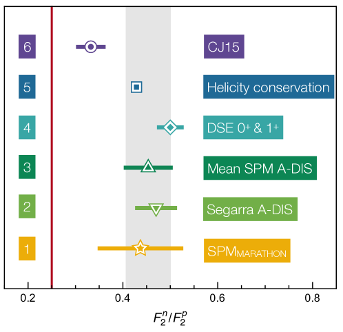
Figure 27: $\lim_{x\to 1}F_{2}^{n}(x)/F_{2}^{p}(x)$. SPM prediction derived from Ref. (Abrams et al., 2022, MARATHON) compared with results inferred from: nuclear DIS Segarra et al. (2020); large-$x$ estimate from CSM studies Segovia et al. (2014); Xu et al. (2015); quark counting (helicity conservation) Farrar and Jackson (1975); and a phenomenological fit (CJ15) Accardi et al. (2016). The red vertical line indicates the Nachtmann lower-limit, Eq. (63), which is saturated if valence $d$-quarks play no material role at $x=1$; and row 3 is the average in Eq. (64).

The following observations serve as a summary of the analyses in Ref. Cui et al. (2022).

Observation A

… Applied to MARATHON data, the SPM yields $\left.F_{2}^{n}/F_{2}^{p}\right|_{x\to 1}=0.437(85)$ $\Rightarrow$ $\left.{\mathpzc d}^{p}/{\mathpzc u}^{p}\right|_{x\to 1}=0.227(100)$. The possibility $\left.{\mathpzc d}^{p}/{\mathpzc u}^{p}\right|_{x\to 1}=0$ is thus excluded with a 98.7% level of confidence; hence, scalar-diquark-only models of proton structure are excluded with equal likelihood. On the other hand, with this same 98.7% level of confidence, the SPM analysis confirms the QCD parton model prediction Farrar and Jackson (1975); Brodsky et al. (1995): ${\mathpzc d}^{p}(x)\propto{\mathpzc u}^{p}(x)$ on $x\simeq 1$.

Observation B

… The value of $\left.F_{2}^{n}/F_{2}^{p}\right|_{x\to 1}$ inferred from nuclear DIS Segarra et al. (2020) agrees with the SPM prediction; hence, they may be averaged to yield

$$\left.F_{2}^{n}/F_{2}^{p}\right|_{x\to 1}^{\rm SPM\,\&\,DIS-A}=0.454\pm 0.047\,.$$ (64)

This result is drawn at row 3 in Fig. 27. It corresponds to

$$\lim_{x\to 1}\frac{{\mathpzc d}^{p}(x)}{{\mathpzc u}^{p}(x)}=0.230\pm 0.057$$ (65)

and entails that the probability that scalar-diquark-only models of proton structure might be consistent with available data is $1/141,000$. In fact, with a high level of confidence, one may discard any proton structure model that delivers a result for $\left.F_{2}^{n}/F_{2}^{p}\right|_{x\to 1}$ that differs significantly from Eq. (64). (As reviewed in Sec. 9, the ratio $g_{A}^{d}/g_{A}^{u}$ places an even harder exclusion bound on scalar-diquark-only models.)

Observation C

… Within uncertainties, the result in Eq. (64) agrees with both: (i) the value obtained by assuming an SU$(4)$-symmetric spin-flavour wave function for the proton and helicity conservation in high-$Q^{2}$ interactions Farrar and Jackson (1975); Brodsky et al. (1995); and (ii) the prediction developed from proton Faddeev wave functions that contain both scalar and axialvector diquarks, with the axialvector contributing approximately 40% of the proton charge Segovia et al. (2014); Xu et al. (2015). (Recall – this was the axialvector diquark fraction built into the analyses in Refs. Chang et al. (2022); Lu et al. (2022).)

Following common practice, Ref. (Lu et al., 2022, Table 2) lists low-order $\zeta=\zeta_{2},\zeta_{3}$ Mellin moments of all proton and pion DFs. Given P1 and the character of the hadron scale, then comparable momentum fractions in the proton and pion are necessarily identical and, as anticipated above, the total sea-quark momentum fraction is shared between the quark flavours in roughly inverse proportion to their infrared dressed-mass, $M_{f}$. Significantly, given that they are predictions, the calculated values of the proton DF moments in Ref. (Lu et al., 2022, Table 2) are in fair agreement with those produced by phenomenological fits – see e.g., Ref. (Hou et al., 2021, Table VI): referred to the CT18 column, the CSM results match at the level of $1.7(1.5)\,\sigma$. Furthermore, within mutual uncertainties, the pion valence-quark DF moments agree with recent lQCD results Joó et al. (2019); Alexandrou et al. (2021).

It is worth emphasising that the quantitative similarities also extend to the $c$ quark: Ref. Lu et al. (2022) predicts $\langle x\rangle_{{\mathpzc c}_{p}}^{\zeta_{2}}=1.32(5)$%, $\langle x\rangle_{{\mathpzc c}_{p}}^{\zeta_{3}}=1.82(6)$%, cf. $1.7(4)$, $2.5(4)$% in Ref. (Ball et al., 2017, Fig. 60). Moreover, the CSM study predicts $\langle x\rangle_{{\mathpzc c}}^{\zeta=1.5\,{\rm GeV}}=0.64(3)$% in both the pion and proton. Regarding the pion, nothing is known about this momentum fraction; and in the proton, phenomenological estimates are inconclusive, ranging from $0$-$2$% (Ball et al., 2017, Fig. 59). Plainly, a significant $c$ quark momentum fraction is obtained under P1 evolution without recourse to “intrinsic charm” Brodsky et al. (1980). This outcome, which is independent of the explicit form of $\alpha_{1\ell}(k^{2})$, potentially challenges the findings in Ref. Ball et al. (2022). Notwithstanding the size of these calculated fractions, we stress that, as apparent in Fig. 25, ${\mathpzc S}^{\pi,p}_{c}(x)$ have sea-quark profiles.

Given these observations, one is led to reevaluate what is meant by intrinsic charm in the proton or any other hadron. With $\zeta_{\cal H}$ being the scale at which valence quasiparticle degrees-of-freedom carry all measurable properties of a given hadron, then the Fock-space components which might be interpreted as intrinsic charm or intrinsic strangeness, etc., are sublimated into the nonperturbatively-computed $\zeta=\zeta_{\cal H}$ Schwinger functions that completely express the bound-state’s structure. In this context, such Fock space components are interpreted as being members of the set of basis eigenvectors representing a free-field light-front Hamiltonian. One may exemplify this by noting that any true QCD solution for the dressed-quark Schwinger function (propagator) must contain infinitely many and all possible contributing Fock space vectors. The putative “intrinsic” components within a bound-state are then revealed by evolving the hadron-scale Schwinger functions to higher scales, whereat an interpretation of data in terms of a Fock space expansion is relevant and practicable. In one study or another, the actual expressions of the characters of intrinsic charm, strangeness, etc., will depend on the sophistication of the kernels used to calculate the hadron scale Schwinger functions. Nevertheless, as highlighted by Ref. Lu et al. (2022), any reasonable kernels will predict that a measurable fraction of the proton’s light-front momentum is carried by the charm quark sea at all resolving scales for which data may be interpreted in terms of DFs.

With a symmetry-preserving framework in hand that has the demonstrated ability to provide simultaneous predictions for the entire array of proton and pion DFs, one is potentially in a position to bring a new order to the study of hadron structure functions. Stringent new tests of the approach, including P1 – see page P1, and the general character of the hadron scale, Eq. (57), will be found in, amongst other things, studies of helicity-dependent DFs. New insights into proton spin structure may then be forthcoming.

12 Conclusion

We have sketched some recent advances in the use of continuum Schwinger function methods (CSMs) to link QCD and hadron observables. The connecting bridge from theory to observation is supported by the three pillars of emergent hadrons mass (EHM): (i) dynamical generation of a gluon mass scale, whose size is roughly one half the proton mass; (ii) existence of a unique, process-independent effective charge, $\hat{\alpha}(k^{2})$, which runs to a finite value at infrared momenta, $\hat{\alpha}(0)/\pi\approx 1$; (iii) and emergence of a running quark mass in the chiral limit, whose infrared value matches that typically identified as the constituent quark mass. Our subsequent commentary stressed that the single phenomenon of EHM manifests itself differently in the diverse array of measurable quantities which define hadron physics. No single observable is alone sufficient to validate the EHM paradigm for understanding strong interactions within the Standard Model (SM). Instead, theory should identify a broad range of empirical consequences of EHM so that the order brought to a collective body of experimental results – existing and future – can be recognised as the signature of EHM.

Our developing understanding of EHM suggests that QCD is unique amongst known fundamental theories of natural phenomena. It might be the first well-defined four-dimensional quantum field theory ever contemplated. If so, then QCD could provide the archetype for theories that take physics beyond the SM.

Science has delivered theories of many things. The best of them remain a part of the grander theories developed in response to new observations. The basic question yet remains unanswered, viz. is there a theory of everything? Hadron physics and QCD might be pointing us toward an answer in exposing the special qualities of strong-coupling non-Abelian quantum gauge field theories.

Work supported by: National Natural Science Foundation of China (grant no. 12135007); and Helmholtz-Zentrum Dresden Rossendorf under the High Potential Programme.

Not applicable.

References

- Appelquist and Pisarski (1981) Appelquist, T.; Pisarski, R.D. High-Temperature Yang-Mills Theories and Three-Dimensional Quantum Chromodynamics. Phys. Rev. D 1981, 23, 2305.
- Appelquist et al. (1986) Appelquist, T.W.; Bowick, M.J.; Karabali, D.; Wijewardhana, L.C.R. Spontaneous Chiral Symmetry Breaking in Three-Dimensional QED. Phys. Rev. D 1986, 33, 3704.
- Bashir et al. (2008) Bashir, A.; Raya, A.; Cloet, I.C.; Roberts, C.D. Regarding confinement and dynamical chiral symmetry breaking in QED3. Phys. Rev. C 2008, 78, 055201.
- Bashir et al. (2009) Bashir, A.; Raya, A.; Sánchez-Madrigal, S.; Roberts, C.D. Gauge invariance of a critical number of flavours in QED3. Few Body Syst. 2009, 46, 229–237.
- Braun et al. (2014) Braun, J.; Gies, H.; Janssen, L.; Roscher, D. Phase structure of many-flavor QED3. Phys. Rev. D 2014, 90, 036002.
- Roberts (2017) Roberts, C.D. Perspective on the origin of hadron masses. Few Body Syst. 2017, 58, 5.
- Glimm and Jaffee (1981) Glimm, J.; Jaffee, A. Quantum Physics. A Functional Point of View; Springer-Verlag, New York, 1981.
- Seiler (1982) Seiler, E. Gauge Theories as a Problem of Constructive Quantum Theory and Statistical Mechanics; Springer-Verlag, New York, 1982.
- Itzykson and Zuber (1980) Itzykson, C.; Zuber, J.B. Quantum Field Theory; McGraw-Hill Inc., New York, 1980.
- Rakow (1991) Rakow, P.E.L. Renormalization group flow in QED: An investigation of the Schwinger-Dyson equations. Nucl. Phys. B 1991, 356, 27–45.
- Gockeler et al. (1995) Gockeler, M.; Horsley, R.; Linke, V.; Rakow, P.E.L.; Schierholz, G.; Stuben, H. Probing the continuum limit in noncompact QED: New results on large lattices. Nucl. Phys. B Proc. Suppl. 1995, 42, 660–662.
- Reenders (2000) Reenders, M. On the nontriviality of Abelian gauged Nambu-Jona-Lasinio models in four dimensions. Phys. Rev. D 2000, 62, 025001.
- Kızılersü et al. (2015) Kızılersü, A.; Sizer, T.; Pennington, M.R.; Williams, A.G.; Williams, R. Dynamical mass generation in unquenched QED using the Dyson-Schwinger equations. Phys. Rev. D 2015, 91, 065015.
- Roberts and Schmidt (2000) Roberts, C.D.; Schmidt, S.M. Dyson-Schwinger equations: Density, temperature and continuum strong QCD. Prog. Part. Nucl. Phys. 2000, 45, S1–S103.
- Roberts et al. (1992) Roberts, C.D.; Williams, A.G.; Krein, G. On the implications of confinement. Int. J. Mod. Phys. A 1992, 7, 5607–5624.
- Roberts and Williams (1994) Roberts, C.D.; Williams, A.G. Dyson-Schwinger equations and their application to hadronic physics. Prog. Part. Nucl. Phys. 1994, 33, 477–575.
- Binosi and Tripolt (2020) Binosi, D.; Tripolt, R.A. Spectral functions of confined particles. Phys. Lett. B 2020, 801, 135171.
- Wilson (1974) Wilson, K.G. Confinement of quarks. Phys. Rev. D 1974, 10, 2445–2459.
- Wilson (2005) Wilson, K.G. The origins of lattice gauge theory. Nucl. Phys. Proc. Suppl. 2005, 140, 3–19.
- Detmold et al. (2022) Detmold, W.; et al. Proceedings of The 38th International Symposium on Lattice Field Theory — PoS(LATTICE2021). PoS 2022, 396.
- Maris and Roberts (2003) Maris, P.; Roberts, C.D. Dyson-Schwinger equations: A tool for hadron physics. Int. J. Mod. Phys. E 2003, 12, 297–365.
- Roberts (2008) Roberts, C.D. Hadron Properties and Dyson-Schwinger Equations. Prog. Part. Nucl. Phys. 2008, 61, 50–65.
- Chang et al. (2011) Chang, L.; Roberts, C.D.; Tandy, P.C. Selected highlights from the study of mesons. Chin. J. Phys. 2011, 49, 955–1004.
- Bashir et al. (2012) Bashir, A.; Chang, L.; Cloet, I.C.; El-Bennich, B.; Liu, Y.X.; Roberts, C.D.; Tandy, P.C. Collective perspective on advances in Dyson-Schwinger Equation QCD. Commun. Theor. Phys. 2012, 58, 79–134.
- Roberts (2015) Roberts, C.D. Strong QCD and Dyson-Schwinger Equations. IRMA Lect. Math. and Theor. Phys. 2015, 21, 356–458.
- Roberts (2016) Roberts, C.D. Three Lectures on Hadron Physics. J. Phys. Conf. Ser. 2016, 706, 022003.
- Horn and Roberts (2016) Horn, T.; Roberts, C.D. The pion: an enigma within the Standard Model. J. Phys. G. 2016, 43, 073001.
- Eichmann et al. (2016) Eichmann, G.; Sanchis-Alepuz, H.; Williams, R.; Alkofer, R.; Fischer, C.S. Baryons as relativistic three-quark bound states. Prog. Part. Nucl. Phys. 2016, 91, 1–100.
- Burkert and Roberts (2019) Burkert, V.D.; Roberts, C.D. Roper resonance: Toward a solution to the fifty-year puzzle. Rev. Mod. Phys. 2019, 91, 011003.
- Fischer (2019) Fischer, C.S. QCD at finite temperature and chemical potential from Dyson–Schwinger equations. Prog. Part. Nucl. Phys. 2019, 105, 1–60.
- Qin and Roberts (2020) Qin, S.X.; Roberts, C.D. Impressions of the Continuum Bound State Problem in QCD. Chin. Phys. Lett. 2020, 37, 121201.
- Roberts and Schmidt (2020) Roberts, C.D.; Schmidt, S.M. Reflections upon the Emergence of Hadronic Mass. Eur. Phys. J. ST 2020, 229, 3319–3340.
- Roberts (2020) Roberts, C.D. Empirical Consequences of Emergent Mass. Symmetry 2020, 12, 1468.
- Roberts (2021) Roberts, C.D. On Mass and Matter. AAPPS Bulletin 2021, 31, 6.
- Roberts et al. (2021) Roberts, C.D.; Richards, D.G.; Horn, T.; Chang, L. Insights into the emergence of mass from studies of pion and kaon structure. Prog. Part. Nucl. Phys. 2021, 120, 103883.
- Binosi (2022) Binosi, D. Emergent Hadron Mass in Strong Dynamics. Few Body Syst. 2022, 63, 42.
- Papavassiliou (2022) Papavassiliou, J. Emergence of mass in the gauge sector of QCD. Chin. Phys. C 2022, 46, 112001.
- Flambaum et al. (2006) Flambaum, V.V.; et al. Sigma terms of light-quark hadrons. Few Body Syst. 2006, 38, 31–51.
- Ruiz de Elvira et al. (2018) Ruiz de Elvira, J.; Hoferichter, M.; Kubis, B.; Meißner, U.G. Extracting the -term from low-energy pion-nucleon scattering. J. Phys. G 2018, 45, 024001.
- Aoki et al. (2020) Aoki, S.; et al. FLAG Review 2019. Eur. Phys. J. C 2020, 80, 113.
- Workman et al. (2022) Workman, R.L.; et al. Review of Particle Physics. PTEP 2022, 2022, 083C01.
- Englert (2014) Englert, F. Nobel Lecture: The BEH mechanism and its scalar boson. Rev. Mod. Phys. 2014, 86, 843.
- Higgs (2014) Higgs, P.W. Nobel Lecture: Evading the Goldstone theorem. Rev. Mod. Phys. 2014, 86, 851.
- Nambu (1960) Nambu, Y. Quasiparticles and Gauge Invariance in the Theory of Superconductivity. Phys. Rev. 1960, 117, 648–663.
- Goldstone (1961) Goldstone, J. Field Theories with Superconductor Solutions. Nuovo Cim. 1961, 19, 154–164.
- Gell-Mann et al. (1968) Gell-Mann, M.; Oakes, R.J.; Renner, B. Behavior of current divergences under SU(3) x SU(3). Phys. Rev. 1968, 175, 2195–2199.
- Casher and Susskind (1974) Casher, A.; Susskind, L. Chiral magnetism (or magnetohadrochironics). Phys. Rev. 1974, D9, 436–460.
- Brodsky and Shrock (2011) Brodsky, S.J.; Shrock, R. Condensates in Quantum Chromodynamics and the Cosmological Constant. Proc. Nat. Acad. Sci. 2011, 108, 45–50.
- Brodsky et al. (2010) Brodsky, S.J.; Roberts, C.D.; Shrock, R.; Tandy, P.C. New perspectives on the quark condensate. Phys. Rev. C 2010, 82, 022201(R).
- Chang et al. (2012) Chang, L.; Roberts, C.D.; Tandy, P.C. Expanding the concept of in-hadron condensates. Phys. Rev. C 2012, 85, 012201(R).
- Brodsky et al. (2012) Brodsky, S.J.; Roberts, C.D.; Shrock, R.; Tandy, P.C. Confinement contains condensates. Phys. Rev. C 2012, 85, 065202.
- Cloet and Roberts (2014) Cloet, I.C.; Roberts, C.D. Explanation and Prediction of Observables using Continuum Strong QCD. Prog. Part. Nucl. Phys. 2014, 77, 1–69.
- Pascual and Tarrach (1984) Pascual, P.; Tarrach, R. QCD: Renormalization for the Practitioner, Lecture Notes in Physics; Vol. 194, Springer-Verlag, Berlin, 1984.
- Taylor (1971) Taylor, J.C. Ward Identities and Charge Renormalization of the Yang-Mills Field. Nucl. Phys. B 1971, 33, 436–444.
- Slavnov (1972) Slavnov, A.A. Ward Identities in Gauge Theories. Theor. Math. Phys. 1972, 10, 99–107.
- Schwinger (1962a) Schwinger, J.S. Gauge Invariance and Mass. Phys. Rev. 1962, 125, 397–398.
- Schwinger (1962b) Schwinger, J.S. Gauge Invariance and Mass. 2. Phys. Rev. 1962, 128, 2425–2429.
- Appelquist et al. (1988) Appelquist, T.; Nash, D.; Wijewardhana, L. Critical Behavior in (2+1)-Dimensional QED. Phys. Rev. Lett. 1988, 60, 2575.
- Maris (1996) Maris, P. The influence of the full vertex and vacuum polarization on the fermion propagator in QED3. Phys. Rev. 1996, D54, 4049–4058.
- Aguilar et al. (2010) Aguilar, A.C.; Binosi, D.; Papavassiliou, J. Nonperturbative gluon and ghost propagators for d=3 Yang-Mills. Phys. Rev. D 2010, 81, 125025.
- Cornwall (2016) Cornwall, J.M. Exploring dynamical gluon mass generation in three dimensions. Phys. Rev. D 2016, 93, 025021.
- Cornwall (1982) Cornwall, J.M. Dynamical Mass Generation in Continuum QCD. Phys. Rev. D 1982, 26, 1453.
- Aguilar et al. (2008) Aguilar, A.C.; Binosi, D.; Papavassiliou, J. Gluon and ghost propagators in the Landau gauge: Deriving lattice results from Schwinger-Dyson equations. Phys. Rev. D 2008, 78, 025010.
- Boucaud et al. (2008) Boucaud, P.; Leroy, J.; Le Yaouanc, A.; Micheli, J.; Pene, O.; Rodríguez-Quintero, J. On the IR behaviour of the Landau-gauge ghost propagator. JHEP 2008, 0806, 099.
- Binosi and Papavassiliou (2009) Binosi, D.; Papavassiliou, J. Pinch Technique: Theory and Applications. Phys. Rept. 2009, 479, 1–152.
- Boucaud et al. (2012) Boucaud, P.; Leroy, J.P.; Le-Yaouanc, A.; Micheli, J.; Pene, O.; Rodríguez-Quintero, J. The Infrared Behaviour of the Pure Yang-Mills Green Functions. Few Body Syst. 2012, 53, 387–436.
- Aguilar et al. (2016) Aguilar, A.C.; Binosi, D.; Papavassiliou, J. The Gluon Mass Generation Mechanism: A Concise Primer. Front. Phys. China 2016, 11, 111203.
- Binosi et al. (2015) Binosi, D.; Chang, L.; Papavassiliou, J.; Roberts, C.D. Bridging a gap between continuum-QCD and ab initio predictions of hadron observables. Phys. Lett. B 2015, 742, 183–188.
- Aguilar et al. (2022) Aguilar, A.C.; Ferreira, M.N.; Papavassiliou, J. Exploring smoking-gun signals of the Schwinger mechanism in QCD. Phys. Rev. D 2022, 105, 014030.
- Pinto-Gómez et al. (2022) Pinto-Gómez, F.; De Soto, F.; Ferreira, M.N.; Papavassiliou, J.; Rodríguez-Quintero, J. Lattice three-gluon vertex in extended kinematics: planar degeneracy – arXiv:2208.01020 [hep-ph] 2022.
- Cui et al. (2020) Cui, Z.F.; Zhang, J.L.; Binosi, D.; de Soto, F.; Mezrag, C.; Papavassiliou, J.; Roberts, C.D.; Rodríguez-Quintero, J.; Segovia, J.; Zafeiropoulos, S. Effective charge from lattice QCD. Chin. Phys. C 2020, 44, 083102.
- Aguilar et al. (2020) Aguilar, A.C.; De Soto, F.; Ferreira, M.; Papavassiliou, J.; Rodríguez-Quintero, J.; Zafeiropoulos, S. Gluon propagator and three-gluon vertex with dynamical quarks. Eur. Phys. J. C 2020, 80, 154.
- Blum et al. (2016) Blum, T.; et al. Domain wall QCD with physical quark masses. Phys. Rev. D 2016, 93, 074505.
- Boyle et al. (2016) Boyle, P.A.; et al. Low energy constants of SU(2) partially quenched chiral perturbation theory from Nf=2+1 domain wall QCD. Phys. Rev. D 2016, 93, 054502.
- Boyle et al. (2017) Boyle, P.A.; Del Debbio, L.; Jüttner, A.; Khamseh, A.; Sanfilippo, F.; Tsang, J.T. The decay constants and in the continuum limit of domain wall lattice QCD. JHEP 2017, 12, 008.
- Binosi et al. (2017) Binosi, D.; Chang, L.; Papavassiliou, J.; Qin, S.X.; Roberts, C.D. Natural constraints on the gluon-quark vertex. Phys. Rev. D 2017, 95, 031501(R).
- Brodsky et al. (2022) Brodsky, S.J.; Deur, A.; Roberts, C.D. Artificial dynamical effects in quantum field theory. Nature Rev. Phys. 2022, 4, 489–495.
- West (1983) West, G.B. General Infrared and Ultraviolet Properties of the Gluon Propagator in Axial Gauge. Phys. Rev. D 1983, 27, 1878.
- Brown and Pennington (1989) Brown, N.; Pennington, M.R. Studies of Confinement: How the Gluon Propagates. Phys. Rev. D 1989, 39, 2723.
- Cucchieri et al. (2009) Cucchieri, A.; Mendes, T.; Santos, E.M.S. Covariant gauge on the lattice: A New implementation. Phys. Rev. Lett. 2009, 103, 141602.
- Gao et al. (2018) Gao, F.; Qin, S.X.; Roberts, C.D.; Rodríguez-Quintero, J. Locating the Gribov horizon. Phys. Rev. D 2018, 97, 034010.
- Gell-Mann and Low (1954) Gell-Mann, M.; Low, F.E. Quantum electrodynamics at small distances. Phys. Rev. 1954, 95, 1300–1312.
- Politzer (2005) Politzer, H.D. The dilemma of attribution. Proc. Nat. Acad. Sci. 2005, 102, 7789–7793.
- Wilczek (2005) Wilczek, F. Asymptotic freedom: From paradox to paradigm. Proc. Nat. Acad. Sci. 2005, 102, 8403–8413.
- Gross (2005) Gross, D.J. The discovery of asymptotic freedom and the emergence of QCD. Proc. Nat. Acad. Sci. 2005, 102, 9099–9108.
- Pickering (1999) Pickering, A. Constructing Quarks. A Sociological History of Particle Physics; University of Chicago Press, 1999.
- Marciano and Pagels (1978) Marciano, W.J.; Pagels, H. Quantum Chromodynamics: A Review. Phys. Rept. 1978, 36, 137.
- Fischer (2006) Fischer, C.S. Infrared properties of QCD from Dyson-Schwinger equations. J. Phys. G 2006, 32, R253–R291.
- Chang and Roberts (2009) Chang, L.; Roberts, C.D. Sketching the Bethe-Salpeter kernel. Phys. Rev. Lett. 2009, 103, 081601.
- Binosi et al. (2017) Binosi, D.; Mezrag, C.; Papavassiliou, J.; Roberts, C.D.; Rodríguez-Quintero, J. Process-independent strong running coupling. Phys. Rev. D 2017, 96, 054026.
- Pilaftsis (1997) Pilaftsis, A. Generalized pinch technique and the background field method in general gauges. Nucl. Phys. B 1997, 487, 467–491.
- Cornwall et al. (2010) Cornwall, J.M.; Papavassiliou, J.; Binosi, D. The Pinch Technique and its Applications to Non-Abelian Gauge Theories; Cambridge University Press, 2010.
- Abbott (1982) Abbott, L.F. Introduction to the Background Field Method. Acta Phys. Polon. B 1982, 13, 33.
- Deur et al. (2016) Deur, A.; Brodsky, S.J.; de Teramond, G.F. The QCD Running Coupling. Prog. Part. Nucl. Phys. 2016, 90, 1–74.
- Deur et al. (2022) Deur, A.; Burkert, V.; Chen, J.P.; Korsch, W. Experimental determination of the QCD effective charge . Particles 2022, 5, 171.
- Deur et al. (2007) Deur, A.; Burkert, V.; Chen, J.P.; Korsch, W. Experimental determination of the effective strong coupling constant. Phys. Lett. B 2007, 650, 244–248.
- Deur et al. (2008) Deur, A.; Burkert, V.; Chen, J.P.; Korsch, W. Determination of the effective strong coupling constant from CLAS spin structure function data. Phys. Lett. B 2008, 665, 349–351.
- Deur et al. (2014) Deur, A.; Prok, Y.; Burkert, V.; Crabb, D.; Girod, F.X.; Griffioen, K.A.; Guler, N.; Kuhn, S.E.; Kvaltine, N. High precision determination of the evolution of the Bjorken Sum. Phys. Rev. D 2014, 90, 012009.
- Ackerstaff et al. (1997) Ackerstaff, K.; et al. Measurement of the neutron spin structure function with a polarized 3He internal target. Phys. Lett. B 1997, 404, 383–389.
- Ackerstaff et al. (1998) Ackerstaff, K.; et al. Determination of the deep inelastic contribution to the generalized Gerasimov-Drell-Hearn integral for the proton and neutron. Phys. Lett. B 1998, 444, 531–538.
- Airapetian et al. (1998) Airapetian, A.; et al. Measurement of the proton spin structure function with a pure hydrogen target. Phys. Lett. B 1998, 442, 484–492.
- Airapetian et al. (2003) Airapetian, A.; et al. Evidence for quark hadron duality in the proton spin asymmetry . Phys. Rev. Lett. 2003, 90, 092002.
- Airapetian et al. (2007) Airapetian, A.; et al. Precise determination of the spin structure function of the proton, deuteron and neutron. Phys. Rev. D 2007, 75, 012007.
- Kim et al. (1998) Kim, J.H.; et al. A Measurement of from the Gross-Llewellyn Smith sum rule. Phys. Rev. Lett. 1998, 81, 3595–3598.
- Alexakhin et al. (2007) Alexakhin, V.Yu.; et al. The Deuteron Spin-dependent Structure Function and its First Moment. Phys. Lett. B 2007, 647, 8–17.
- Alekseev et al. (2010) Alekseev, M.G.; et al. The Spin-dependent Structure Function of the Proton and a Test of the Bjorken Sum Rule. Phys. Lett. B 2010, 690, 466–472.
- Adolph et al. (2016) Adolph, C.; et al. The spin structure function of the proton and a test of the Bjorken sum rule. Phys. Lett. B 2016, 753, 18–28.
- Anthony et al. (1993) Anthony, P.L.; et al. Determination of the neutron spin structure function. Phys. Rev. Lett. 1993, 71, 959–962.
- Abe et al. (1995a) Abe, K.; et al. Precision measurement of the proton spin structure function . Phys. Rev. Lett. 1995, 74, 346–350.
- Abe et al. (1995b) Abe, K.; et al. Precision measurement of the deuteron spin structure function . Phys. Rev. Lett. 1995, 75, 25–28.
- Abe et al. (1996) Abe, K.; et al. Measurements of the proton and deuteron spin structure function and asymmetry . Phys. Rev. Lett. 1996, 76, 587–591.
- Abe et al. (1995) Abe, K.; et al. Measurements of the dependence of the proton and deuteron spin structure functions and . Phys. Lett. B 1995, 364, 61–68.
- Anthony et al. (1996) Anthony, P.L.; et al. Deep inelastic scattering of polarized electrons by polarized 3He and the study of the neutron spin structure. Phys. Rev. D 1996, 54, 6620–6650.
- Abe et al. (1997a) Abe, K.; et al. Precision determination of the neutron spin structure function . Phys. Rev. Lett. 1997, 79, 26–30.
- Abe et al. (1997b) Abe, K.; et al. Measurement of the neutron spin structure function and asymmetry . Phys. Lett. B 1997, 404, 377–382.
- Abe et al. (1997c) Abe, K.; et al. Next-to-leading order QCD analysis of polarized deep inelastic scattering data. Phys. Lett. B 1997, 405, 180–190.
- Abe et al. (1998) Abe, K.; et al. Measurements of the proton and deuteron spin structure functions and . Phys. Rev. 1998, D58, 112003.
- Anthony et al. (1999a) Anthony, P.L.; et al. Measurement of the proton and deuteron spin structure functions and asymmetry . Phys. Lett. 1999, B458, 529–535.
- Anthony et al. (1999b) Anthony, P.L.; et al. Measurement of the deuteron spin structure function for . Phys. Lett. B 1999, 463, 339–345.
- Anthony et al. (2000) Anthony, P.L.; et al. Measurements of the dependence of the proton and neutron spin structure functions and . Phys. Lett. B 2000, 493, 19–28.
- Anthony et al. (2003) Anthony, P.L.; et al. Precision measurement of the proton and deuteron spin structure functions and asymmetries . Phys. Lett. B 2003, 553, 18–24.
- Binosi and Quadri (2013) Binosi, D.; Quadri, A. Anti-BRST symmetry and background field method. Phys. Rev. D 2013, 88, 085036.
- Aslam et al. (2016) Aslam, M.J.; Bashir, A.; Gutierrez-Guerrero, L.X. Local Gauge Transformation for the Quark Propagator in an SU(N) Gauge Theory. Phys. Rev. D 2016, 93, 076001.
- Ding et al. (2020a) Ding, M.; Raya, K.; Binosi, D.; Chang, L.; Roberts, C.D.; Schmidt, S.M. Drawing insights from pion parton distributions. Chin. Phys. C (Lett.) 2020, 44, 031002.
- Ding et al. (2020b) Ding, M.; Raya, K.; Binosi, D.; Chang, L.; Roberts, C.D.; Schmidt, S.M. Symmetry, symmetry breaking, and pion parton distributions. Phys. Rev. D 2020, 101, 054014.
- Cui et al. (2021) Cui, Z.F.; Ding, M.; Gao, F.; Raya, K.; Binosi, D.; Chang, L.; Roberts, C.D.; Rodríguez-Quintero, J.; Schmidt, S.M. Higgs modulation of emergent mass as revealed in kaon and pion parton distributions. Eur. Phys. J. A (Lett.) 2021, 57, 5.
- Cui et al. (2020) Cui, Z.F.; Ding, M.; Gao, F.; Raya, K.; Binosi, D.; Chang, L.; Roberts, C.D.; Rodríguez-Quintero, J.; Schmidt, S.M. Kaon and pion parton distributions. Eur. Phys. J. C 2020, 80, 1064.
- Han et al. (2021) Han, C.; Xie, G.; Wang, R.; Chen, X. An Analysis of Parton Distribution Functions of the Pion and the Kaon with the Maximum Entropy Input. Eur. Phys. J. C 2021, 81, 302.
- Chang and Roberts (2021) Chang, L.; Roberts, C.D. Regarding the distribution of glue in the pion. Chin. Phys. Lett. 2021, 38, 081101.
- Xie et al. (2022) Xie, G.; Han, C.; Wang, R.; Chen, X. Tackling the kaon structure function at EicC. Chin. Phys. C 2022, 46, 064107.
- Raya et al. (2022) Raya, K.; Cui, Z.F.; Chang, L.; Morgado, J.M.; Roberts, C.D.; Rodríguez-Quintero, J. Revealing pion and kaon structure via generalised parton distributions. Chin. Phys. C 2022, 46, 013105.
- Cui et al. (2022a) Cui, Z.F.; Ding, M.; Morgado, J.M.; Raya, K.; Binosi, D.; Chang, L.; Papavassiliou, J.; Roberts, C.D.; Rodríguez-Quintero, J.; Schmidt, S.M. Concerning pion parton distributions. Eur. Phys. J. A 2022, 58, 10.
- Cui et al. (2022b) Cui, Z.F.; Ding, M.; Morgado, J.M.; Raya, K.; Binosi, D.; Chang, L.; De Soto, F.; Roberts, C.D.; Rodríguez-Quintero, J.; Schmidt, S.M. Emergence of pion parton distributions. Phys. Rev. D 2022, 105, L091502.
- Chang et al. (2022) Chang, L.; Gao, F.; Roberts, C.D. Parton distributions of light quarks and antiquarks in the proton. Phys. Lett. B 2022, 829, 137078.
- Lu et al. (2022) Lu, Y.; Chang, L.; Raya, K.; Roberts, C.D.; Rodríguez-Quintero, J. Proton and pion distribution functions in counterpoint. Phys. Lett. B 2022, 830, 137130.
- de Paula et al. (2022) de Paula, W.; Ydrefors, E.; Nogueira Alvarenga, J.H.; Frederico, T.; Salmè, G. Parton distribution function in a pion with Minkowskian dynamics. Phys. Rev. D 2022, 105, L071505.
- Grunberg (1984) Grunberg, G. Renormalization Scheme Independent QCD and QED: The Method of Effective Charges. Phys. Rev. D 1984, 29, 2315.
- Grunberg (1989) Grunberg, G. On Some Ambiguities in the Method of Effective Charges. Phys. Rev. D 1989, 40, 680.
- Dokshitzer (1998) Dokshitzer, Y.L. Perturbative QCD theory (includes our knowledge of ) - hep-ph/9812252. In Proceedings of the High-energy physics. Proceedings, 29th International Conference, ICHEP’98, Vancouver, Canada, July 23-29, 1998. Vol. 1, 2, 1998, pp. 305–324.
- Prosperi et al. (2007) Prosperi, G.M.; Raciti, M.; Simolo, C. On the running coupling constant in QCD. Prog. Part. Nucl. Phys. 2007, 58, 387–438.
- Bjorken (1966) Bjorken, J.D. Applications of the Chiral U(6) x (6) Algebra of Current Densities. Phys. Rev. 1966, 148, 1467–1478.
- Bjorken (1970) Bjorken, J.D. Inelastic Scattering of Polarized Leptons from Polarized Nucleons. Phys. Rev. D 1970, 1, 1376–1379.
- Brodsky and de Téramond (2004) Brodsky, S.J.; de Téramond, G.F. Light-front hadron dynamics and AdS/CFT correspondence. Phys. Lett. B 2004, 582, 211–221.
- Brodsky et al. (2010) Brodsky, S.J.; de Teramond, G.F.; Deur, A. Nonperturbative QCD Coupling and its -function from Light-Front Holography. Phys. Rev. D 2010, 81, 096010.
- Carlson et al. (2006) Carlson, J.; Jaffe, A.; Wiles, A., Eds. The Millennium Prize Problems; American Mathematical Society, Providence, 2006.
- Eichten et al. (1978) Eichten, E.; Gottfried, K.; Kinoshita, T.; Lane, K.D.; Yan, T.M. Charmonium: The Model. Phys. Rev. D 1978, 17, 3090. [Erratum: Phys. Rev. D 21, 313 (1980)].
- Richardson (1979) Richardson, J.L. The Heavy Quark Potential and the Upsilon, J/psi Systems. Phys. Lett. B 1979, 82, 272–274.
- Buchmuller and Tye (1981) Buchmuller, W.; Tye, S.H.H. Quarkonia and Quantum Chromodynamics. Phys. Rev. D 1981, 24, 132.
- Godfrey and Isgur (1985) Godfrey, S.; Isgur, N. Mesons in a Relativized Quark Model with Chromodynamics. Phys. Rev. D 1985, 32, 189–231.
- Lucha et al. (1991) Lucha, W.; Schöberl, F.F.; Gromes, D. Bound states of quarks. Phys. Rept. 1991, 200, 127–240.
- Binosi et al. (2016) Binosi, D.; Chang, L.; Qin, S.X.; Papavassiliou, J.; Roberts, C.D. Symmetry preserving truncations of the gap and Bethe-Salpeter equations. Phys. Rev. D 2016, 93, 096010.
- Smirnov et al. (2010) Smirnov, A.V.; Smirnov, V.A.; Steinhauser, M. Three-loop static potential. Phys. Rev. Lett. 2010, 104, 112002.
- Brodsky et al. (2015a) Brodsky, S.J.; Deur, A.; de Téramond, G.F.; Dosch, H.G. Light-Front Holography and Superconformal Quantum Mechanics: A New Approach to Hadron Structure and Color Confinement. Int. J. Mod. Phys. Conf. Ser. 2015, 39, 1560081.
- Brodsky et al. (2015b) Brodsky, S.J.; de Teramond, G.F.; Dosch, H.G.; Erlich, J. Light-Front Holographic QCD and Emerging Confinement. Phys. Rept. 2015, 584, 1–105.
- Reinhardt et al. (2018) Reinhardt, H.; Burgio, G.; Campagnari, D.; Ebadati, E.; Heffner, J.; Quandt, M.; Vastag, P.; Vogt, H. Hamiltonian approach to QCD in Coulomb gauge - a survey of recent results. Adv. High Energy Phys. 2018, 2018, 2312498.
- Hoyer (2021) Hoyer, P. Journey to the Bound States; SpringerBriefs in Physics, Springer, 2021.
- Bali et al. (2005) Bali, G.S.; Neff, H.; Duessel, T.; Lippert, T.; Schilling, K. Observation of string breaking in QCD. Phys. Rev. D 2005, 71, 114513.
- Prkacin et al. (2006) Prkacin, Z.; Bali, G.S.; Dussel, T.; Lippert, T.; Neff, H.; Schilling, K. Anatomy of string breaking in QCD. PoS 2006, LAT2005, 308.
- Chang et al. (2009) Chang, L.; Cloet, I.C.; El-Bennich, B.; Klähn, T.; Roberts, C.D. Exploring the light-quark interaction. Chin. Phys. C 2009, 33, 1189–1196.
- Munczek and Nemirovsky (1983) Munczek, H.J.; Nemirovsky, A.M. The Ground State Mass Spectrum in QCD. Phys. Rev. D 1983, 28, 181–186.
- Stingl (1986) Stingl, M. Propagation Properties and Condensate Formation of the Confined Yang-Mills Field. Phys. Rev. D 1986, 34, 3863–3881. [Erratum: Phys. Rev. D 36, 651 (1987)].
- Zwanziger (1989) Zwanziger, D. Local and Renormalizable Action From the Gribov Horizon. Nucl. Phys. B 1989, 323, 513–544.
- Burden et al. (1992) Burden, C.J.; Roberts, C.D.; Williams, A.G. Singularity structure of a model quark propagator. Phys. Lett. B 1992, 285, 347–353.
- Gribov (1999) Gribov, V.N. The theory of quark confinement. Eur. Phys. J. C 1999, 10, 91–105.
- Stingl (1996) Stingl, M. A Systematic extended iterative solution for quantum chromodynamics. Z. Phys. A 1996, 353, 423–445.
- Dudal et al. (2008) Dudal, D.; Gracey, J.A.; Sorella, S.P.; Vandersickel, N.; Verschelde, H. A Refinement of the Gribov-Zwanziger approach in the Landau gauge: Infrared propagators in harmony with the lattice results. Phys. Rev. D 2008, 78, 065047.
- Qin and Rischke (2013) Qin, S.X.; Rischke, D.H. Quark Spectral Function and Deconfinement at Nonzero Temperature. Phys. Rev. D 2013, 88, 056007.
- Lucha and Schöberl (2016) Lucha, W.; Schöberl, F.F. Analytic Bethe-Salpeter Description of the Lightest Pseudoscalar Mesons. Phys. Rev. D 2016, 93, 056006.
- Dudal et al. (2020) Dudal, D.; Oliveira, O.; Roelfs, M.; Silva, P. Spectral representation of lattice gluon and ghost propagators at zero temperature. Nucl. Phys. B 2020, 952, 114912.
- Fischer and Huber (2020) Fischer, C.S.; Huber, M.Q. Landau gauge Yang-Mills propagators in the complex momentum plane. Phys. Rev. D 2020, 102, 094005.
- Osterwalder and Schrader (1973) Osterwalder, K.; Schrader, R. Axioms for Euclidean Green’s Functions. Commun. Math. Phys. 1973, 31, 83–112.
- Osterwalder and Schrader (1975) Osterwalder, K.; Schrader, R. Axioms for Euclidean Green’s Functions. 2. Commun. Math. Phys. 1975, 42, 281.
- Dedushenko (2022) Dedushenko, M. Snowmass White Paper: The Quest to Define QFT – arXiv:2203.08053 [hep-ph] 2022.
- Stodolna et al. (2013) Stodolna, A.S.; Rouzée, A.; Lépine, F.; Cohen, S.; Robicheaux, F.; Gijsbertsen, A.; Jungmann, J.H.; Bordas, C.; Vrakking, M.J.J. Hydrogen Atoms under Magnification: Direct Observation of the Nodal Structure of Stark States. Phys. Rev. Lett. 2013, 110, 213001.
- Bhagwat et al. (2003) Bhagwat, M.; Pichowsky, M.; Tandy, P.C. Confinement phenomenology in the Bethe-Salpeter equation. Phys. Rev. D 2003, 67, 054019.
- Field and Feynman (1978) Field, R.D.; Feynman, R.P. A Parametrization of the Properties of Quark Jets. Nucl. Phys. B 1978, 136, 1–76.
- Gribov and Lipatov (1971) Gribov, V.N.; Lipatov, L.N. Deep inelastic electron scattering in perturbation theory. Phys. Lett. B 1971, 37, 78–80.
- Brodsky et al. (2015) Brodsky, S.J.; Deshpande, A.L.; Gao, H.; McKeown, R.D.; Meyer, C.A.; Meziani, Z.E.; Milner, R.G.; Qiu, J.; Richards, D.G.; Roberts, C.D. QCD and Hadron Physics – arXiv:1502.05728 [hep-ph] 2015.
- Denisov et al. (2018) Denisov, O.; et al. Letter of Intent (Draft 2.0): A New QCD facility at the M2 beam line of the CERN SPS 2018.
- Aguilar et al. (2019) Aguilar, A.C.; et al. Pion and Kaon Structure at the Electron-Ion Collider. Eur. Phys. J. A 2019, 55, 190.
- Brodsky et al. (2020) Brodsky, S.J.; et al. Strong QCD from Hadron Structure Experiments. Int. J. Mod. Phys. E 2020, 29, 2030006.
- Chen et al. (2020) Chen, X.; Guo, F.K.; Roberts, C.D.; Wang, R. Selected Science Opportunities for the EicC. Few Body Syst. 2020, 61, 43.
- Anderle et al. (2021) Anderle, D.P.; et al. Electron-ion collider in China. Front. Phys. (Beijing) 2021, 16, 64701.
- Arrington et al. (2021) Arrington, J.; et al. Revealing the structure of light pseudoscalar mesons at the electron–ion collider. J. Phys. G 2021, 48, 075106.
- Aoki et al. (2021) Aoki, K.; et al. Extension of the J-PARC Hadron Experimental Facility: Third White Paper – arXiv:2110.04462 [nucl-ex] 2021. Extension of the J-PARC Hadron Experimental Facility: Third White Paper – arXiv:2110.04462 [nucl-ex].
- Quintans (2022) Quintans, C. The New AMBER Experiment at the CERN SPS. Few Body Syst. 2022, 63, 72.
- Capstick and Roberts (2000) Capstick, S.; Roberts, W. Quark models of baryon masses and decays. Prog. Part. Nucl. Phys. 2000, 45, S241–S331.
- Giannini and Santopinto (2015) Giannini, M.M.; Santopinto, E. The hypercentral Constituent Quark Model and its application to baryon properties. Chin. J. Phys. 2015, 53, 020301.
- Plessas (2015) Plessas, W. The constituent-quark model — Nowadays. Int. J. Mod. Phys. A 2015, 30, 1530013.
- Dudek et al. (2010) Dudek, J.J.; Edwards, R.G.; Peardon, M.J.; Richards, D.G.; Thomas, C.E. Toward the excited meson spectrum of dynamical QCD. Phys. Rev. D 2010, 82, 034508.
- Edwards et al. (2011) Edwards, R.G.; Dudek, J.J.; Richards, D.G.; Wallace, S.J. Excited state baryon spectroscopy from lattice QCD. Phys. Rev. D 2011, 84, 074508.
- Liu et al. (2012) Liu, L.; Moir, G.; Peardon, M.; Ryan, S.M.; Thomas, C.E.; Vilaseca, P.; Dudek, J.J.; Edwards, R.G.; Joo, B.; Richards, D.G. Excited and exotic charmonium spectroscopy from lattice QCD. JHEP 2012, 07, 126.
- Dudek and Edwards (2012) Dudek, J.J.; Edwards, R.G. Hybrid Baryons in QCD. Phys. Rev. D 2012, 85, 054016.
- Ryan and Wilson (2021) Ryan, S.M.; Wilson, D.J. Excited and exotic bottomonium spectroscopy from lattice QCD. JHEP 2021, 02, 214.
- Woss et al. (2021) Woss, A.J.; Dudek, J.J.; Edwards, R.G.; Thomas, C.E.; Wilson, D.J. Decays of an exotic hybrid meson resonance in QCD. Phys. Rev. D 2021, 103, 054502.
- Munczek (1995) Munczek, H.J. Dynamical chiral symmetry breaking, Goldstone’s theorem and the consistency of the Schwinger-Dyson and Bethe-Salpeter Equations. Phys. Rev. D 1995, 52, 4736–4740.
- Bender et al. (1996) Bender, A.; Roberts, C.D.; von Smekal, L. Goldstone Theorem and Diquark Confinement Beyond Rainbow- Ladder Approximation. Phys. Lett. B 1996, 380, 7–12.
- Maris et al. (1998) Maris, P.; Roberts, C.D.; Tandy, P.C. Pion mass and decay constant. Phys. Lett. B 1998, 420, 267–273.
- Maris and Roberts (1997) Maris, P.; Roberts, C.D. and meson Bethe-Salpeter amplitudes. Phys. Rev. C 1997, 56, 3369–3383.
- Chen et al. (2018) Chen, M.; Ding, M.; Chang, L.; Roberts, C.D. Mass-dependence of pseudoscalar meson elastic form factors. Phys. Rev. D 2018, 98, 091505(R).
- Ding et al. (2019) Ding, M.; Raya, K.; Bashir, A.; Binosi, D.; Chang, L.; Chen, M.; Roberts, C.D. transition form factors. Phys. Rev. D 2019, 99, 014014.
- Eichmann et al. (2020) Eichmann, G.; Fischer, C.S.; Williams, R. Kaon-box contribution to the anomalous magnetic moment of the muon. Phys. Rev. D 2020, 101, 054015.
- Xu et al. (2019) Xu, Y.Z.; Binosi, D.; Cui, Z.F.; Li, B.L.; Roberts, C.D.; Xu, S.S.; Zong, H.S. Elastic electromagnetic form factors of vector mesons. Phys. Rev. D 2019, 100, 114038.
- Xu et al. (2021) Xu, Y.Z.; Chen, S.; Yao, Z.Q.; Binosi, D.; Cui, Z.F.; Roberts, C.D. Vector-meson production and vector meson dominance. Eur. Phys. J. C 2021, 81, 895.
- Yao et al. (2020) Yao, Z.Q.; Binosi, D.; Cui, Z.F.; Roberts, C.D.; Xu, S.S.; Zong, H.S. Semileptonic decays of mesons. Phys. Rev. D 2020, 102, 014007.
- Yao et al. (2021) Yao, Z.Q.; Binosi, D.; Cui, Z.F.; Roberts, C.D. Semileptonic transitions. Phys. Lett. B 2021, 818, 136344.
- Yao et al. (2022) Yao, Z.Q.; Binosi, D.; Cui, Z.F.; Roberts, C.D. Semileptonic transitions: ; ; ; and . Phys. Lett. B 2022, 824, 136793.
- Höll et al. (2004) Höll, A.; Krassnigg, A.; Roberts, C.D. Pseudoscalar meson radial excitations. Phys. Rev. C 2004, 70, 042203(R).
- Höll et al. (2005) Höll, A.; Krassnigg, A.; Maris, P.; Roberts, C.D.; Wright, S.V. Electromagnetic properties of ground and excited state pseudoscalar mesons. Phys. Rev. C 2005, 71, 065204.
- Fischer and Williams (2009) Fischer, C.S.; Williams, R. Probing the gluon self-interaction in light mesons. Phys. Rev. Lett. 2009, 103, 122001.
- Krassnigg (2009) Krassnigg, A. Survey of J=0,1 mesons in a Bethe-Salpeter approach. Phys. Rev. D 2009, 80, 114010.
- Qin et al. (2011) Qin, S.X.; Chang, L.; Liu, Y.X.; Roberts, C.D.; Wilson, D.J. Interaction model for the gap equation. Phys. Rev. C 2011, 84, 042202(R).
- Qin et al. (2012) Qin, S.X.; Chang, L.; Liu, Y.X.; Roberts, C.D.; Wilson, D.J. Investigation of rainbow-ladder truncation for excited and exotic mesons. Phys. Rev. C 2012, 85, 035202.
- Blank and Krassnigg (2011) Blank, M.; Krassnigg, A. Bottomonium in a Bethe-Salpeter-equation study. Phys. Rev. D 2011, 84, 096014.
- Hilger et al. (2015) Hilger, T.; Popovici, C.; Gomez-Rocha, M.; Krassnigg, A. Spectra of heavy quarkonia in a Bethe-Salpeter-equation approach. Phys. Rev. D 2015, 91, 034013.
- Fischer et al. (2015) Fischer, C.S.; Kubrak, S.; Williams, R. Spectra of heavy mesons in the Bethe-Salpeter approach. Eur. Phys. J. A 2015, 51, 10.
- Eichmann et al. (2016) Eichmann, G.; Fischer, C.S.; Sanchis-Alepuz, H. Light baryons and their excitations. Phys. Rev. D 2016, 94, 094033.
- Qin et al. (2019) Qin, S.X.; Roberts, C.D.; Schmidt, S.M. Spectrum of light- and heavy-baryons. Few Body Syst. 2019, 60, 26.
- Chang and Roberts (2012) Chang, L.; Roberts, C.D. Tracing masses of ground-state light-quark mesons. Phys. Rev. C 2012, 85, 052201(R).
- Williams et al. (2016) Williams, R.; Fischer, C.S.; Heupel, W. Light mesons in QCD and unquenching effects from the 3PI effective action. Phys. Rev. D 2016, 93, 034026.
- Qin and Roberts (2021) Qin, S.X.; Roberts, C.D. Resolving the Bethe-Salpeter kernel. Chin. Phys. Lett. Express 2021, 38, 071201.
- Xu et al. (2022) Xu, Z.N.; Yao, Z.Q.; Qin, S.X.; Cui, Z.F.; Roberts, C.D. Bethe-Salpeter kernel and properties of strange-quark mesons – arXiv:2208.13903 [hep-ph] 2022.
- Qin et al. (2014) Qin, S.X.; Roberts, C.D.; Schmidt, S.M. Ward-Green-Takahashi identities and the axial-vector vertex. Phys. Lett. B 2014, 733, 202–208.
- Bhagwat et al. (2004) Bhagwat, M.S.; Höll, A.; Krassnigg, A.; Roberts, C.D.; Tandy, P.C. Aspects and consequences of a dressed-quark-gluon vertex. Phys. Rev. C 2004, 70, 035205.
- Chang et al. (2009) Chang, L.; Liu, Y.X.; Roberts, C.D.; Shi, Y.M.; Sun, W.M.; Zong, H.S. Chiral susceptibility and the scalar Ward identity. Phys. Rev. C 2009, 79, 035209.
- Singh (1985) Singh, J. Anomalous magnetic moment of light quarks and dynamical symmetry breaking. Phys. Rev. D 1985, 31, 1097–1108.
- Bicudo et al. (1999) Bicudo, P.J.A.; Ribeiro, J.E.F.T.; Fernandes, R. The anomalous magnetic moment of quarks. Phys. Rev. C 1999, 59, 1107–1112.
- Chang et al. (2011) Chang, L.; Liu, Y.X.; Roberts, C.D. Dressed-quark anomalous magnetic moments. Phys. Rev. Lett. 2011, 106, 072001.
- Bashir et al. (2012) Bashir, A.; Bermúdez, R.; Chang, L.; Roberts, C.D. Dynamical chiral symmetry breaking and the fermion–gauge-boson vertex. Phys. Rev. C 2012, 85, 045205.
- Kızılersü et al. (2021) Kızılersü, A.; Oliveira, O.; Silva, P.J.; Skullerud, J.I.; Sternbeck, A. Quark-gluon vertex from lattice QCD. Phys. Rev. D 2021, 103, 114515.
- Williams (2015) Williams, R. The quark-gluon vertex in Landau gauge bound-state studies. Eur. Phys. J. A 2015, 51, 57.
- Yin et al. (2021) Yin, P.L.; Cui, Z.F.; Roberts, C.D.; Segovia, J. Masses of positive- and negative-parity hadron ground-states, including those with heavy quarks. Eur. Phys. J. C 2021, 81, 327.
- Xu et al. (2021) Xu, Z.N.; Cui, Z.F.; Roberts, C.D.; Xu, C. Heavy + light pseudoscalar meson semileptonic transitions. Eur. Phys. J. C 2021, 81, 1105.
- Gutiérrez-Guerrero et al. (2021) Gutiérrez-Guerrero, L.X.; Paredes-Torres, G.; Bashir, A. Mesons and baryons: Parity partners. Phys. Rev. D 2021, 104, 094013.
- Höll et al. (2006) Höll, A.; Maris, P.; Roberts, C.D.; Wright, S.V. Schwinger functions and light-quark bound states, and sigma terms. Nucl. Phys. Proc. Suppl. 2006, 161, 87–94.
- Santowsky et al. (2020) Santowsky, N.; Eichmann, G.; Fischer, C.S.; Wallbott, P.C.; Williams, R. The -meson: four-quark vs. two-quark components and decay width in a Bethe-Salpeter approach. Phys. Rev. D 2020, 102, 056014.
- Cui et al. (2022) Cui, Z.F.; Binosi, D.; Roberts, C.D.; Schmidt, S.M. Hadron and light nucleus radii from electron scattering. Chin. Phys. C 2022, 46, 122001.
- Binosi et al. (2019) Binosi, D.; Chang, L.; Ding, M.; Gao, F.; Papavassiliou, J.; Roberts, C.D. Distribution Amplitudes of Heavy-Light Mesons. Phys. Lett. B 2019, 790, 257–262.
- Nakanishi (1969) Nakanishi, N. A General survey of the theory of the Bethe-Salpeter equation. Prog. Theor. Phys. Suppl. 1969, 43, 1–81.
- McNeile and Michael (2006) McNeile, C.; Michael, C. The decay constant of the first excited pion from lattice QCD. Phys. Lett. B 2006, 642, 244–247.
- Ballon-Bayona et al. (2015) Ballon-Bayona, A.; Krein, G.; Miller, C. Decay constants of the pion and its excitations in holographic QCD. Phys. Rev. D 2015, 91, 065024.
- Chen and Chang (2019) Chen, M.; Chang, L. A pattern for the flavor dependent quark-antiquark interaction. Chin. Phys. C 2019, 43, 114103.
- Qin et al. (2020) Qin, P.; Qin, S.X.; Liu, Y.X. Heavy-light mesons beyond the ladder approximation. Phys. Rev. D 2020, 101, 114014.
- Burden and Pichowsky (2002) Burden, C.J.; Pichowsky, M.A. exotic mesons from the Bethe-Salpeter equation. Few Body Syst. 2002, 32, 119–126.
- Hilger et al. (2015) Hilger, T.; Gomez-Rocha, M.; Krassnigg, A. Masses of exotic quarkonia in a Bethe-Salpeter-equation approach. Phys. Rev. D 2015, 91, 114004.
- Xu et al. (2019) Xu, S.S.; Cui, Z.F.; Chang, L.; Papavassiliou, J.; Roberts, C.D.; Zong, H.S. New perspective on hybrid mesons. Eur. Phys. J. A (Lett.) 2019, 55, 113.
- Meyers and Swanson (2013) Meyers, J.; Swanson, E.S. Spin Zero Glueballs in the Bethe-Salpeter Formalism. Phys. Rev. D 2013, 87, 036009.
- Souza et al. (2020) Souza, E.V.; Narciso Ferreira, M.; Aguilar, A.C.; Papavassiliou, J.; Roberts, C.D.; Xu, S.S. Pseudoscalar glueball mass: a window on three-gluon interactions. Eur. Phys. J. A (Lett.) 2020, 56, 25.
- Kaptari and Kämpfer (2020) Kaptari, L.P.; Kämpfer, B. Mass spectrum of pseudo-scalar glueballs from a Bethe-Salpeter approach with the rainbow-ladder truncation. Few Body Syst. 2020, 61, 28.
- Huber et al. (2021) Huber, M.Q.; Fischer, C.S.; Sanchis-Alepuz, H. Higher spin glueballs from functional methods. Eur. Phys. J. C 2021, 81, 1083.
- Ablikim et al. (2020) Ablikim, M.; et al. Future Physics Programme of BESIII. Chin. Phys. C 2020, 44, 040001.
- Abdul Khalek et al. (2022) Abdul Khalek, R.; et al. Science Requirements and Detector Concepts for the Electron-Ion Collider: EIC Yellow Report. Nucl. Phys. A 2022, 1026, 122447.
- Pauli (2022) Pauli, P. Accessing glue through photoproduction measurements at GlueX. Rev. Mex. Fis. Suppl. 2022, 3, 0308002.
- Eichmann et al. (2010) Eichmann, G.; Alkofer, R.; Krassnigg, A.; Nicmorus, D. Nucleon mass from a covariant three-quark Faddeev equation. Phys. Rev. Lett. 2010, 104, 201601.
- Barabanov et al. (2021) Barabanov, M.Y.; et al. Diquark Correlations in Hadron Physics: Origin, Impact and Evidence. Prog. Part. Nucl. Phys. 2021, 116, 103835.
- Cahill et al. (1989) Cahill, R.T.; Roberts, C.D.; Praschifka, J. Baryon structure and QCD. Austral. J. Phys. 1989, 42, 129–145.
- Burden et al. (1989) Burden, C.J.; Cahill, R.T.; Praschifka, J. Baryon Structure and QCD: Nucleon Calculations. Austral. J. Phys. 1989, 42, 147–159.
- Reinhardt (1990) Reinhardt, H. Hadronization of Quark Flavor Dynamics. Phys. Lett. B 1990, 244, 316–326.
- Efimov et al. (1990) Efimov, G.V.; Ivanov, M.A.; Lyubovitskij, V.E. Quark - diquark approximation of the three quark structure of baryons in the quark confinement model. Z. Phys. C 1990, 47, 583–594.
- Gutiérrez-Guerrero et al. (2010) Gutiérrez-Guerrero, L.X.; Bashir, A.; Cloet, I.C.; Roberts, C.D. Pion form factor from a contact interaction. Phys. Rev. C 2010, 81, 065202.
- Gutiérrez-Guerrero and Bashir (2022) Gutiérrez-Guerrero, L.X.; Bashir, A. Contact Interaction Studies of Hadron Observables. Particles 2022, 5, xxx.
- Brown et al. (2014) Brown, Z.S.; Detmold, W.; Meinel, S.; Orginos, K. Charmed bottom baryon spectroscopy from lattice QCD. Phys. Rev. D 2014, 90, 094507.
- Mathur et al. (2018) Mathur, N.; Padmanath, M.; Mondal, S. Precise predictions of charmed-bottom hadrons from lattice QCD. Phys. Rev. Lett. 2018, 121, 202002.
- Bahtiyar et al. (2020) Bahtiyar, H.; Can, K.U.; Erkol, G.; Gubler, P.; Oka, M.; Takahashi, T.T. Charmed baryon spectrum from lattice QCD near the physical point. Phys. Rev. D 2020, 102, 054513.
- Chen et al. (2018) Chen, C.; El-Bennich, B.; Roberts, C.D.; Schmidt, S.M.; Segovia, J.; Wan, S. Structure of the nucleon’s low-lying excitations. Phys. Rev. D 2018, 97, 034016.
- Chen et al. (2019) Chen, C.; Krein, G.I.; Roberts, C.D.; Schmidt, S.M.; Segovia, J. Spectrum and structure of octet and decuplet baryons and their positive-parity excitations. Phys. Rev. D 2019, 100, 054009.
- Liu et al. (2022a) Liu, L.; Chen, C.; Lu, Y.; Roberts, C.D.; Segovia, J. Composition of low-lying -baryons. Phys. Rev. D 2022, 105, 114047.
- Liu et al. (2022b) Liu, L.; Chen, C.; Roberts, C.D. Wave functions of baryons – arXiv:2208.12353 [hep-ph] 2022.
- Crede and Roberts (2013) Crede, V.; Roberts, W. Progress towards understanding baryon resonances. Rept. Prog. Phys. 2013, 76, 076301.
- Alkofer et al. (2005) Alkofer, R.; Höll, A.; Kloker, M.; Krassnigg, A.; Roberts, C.D. On nucleon electromagnetic form-factors. Few Body Syst. 2005, 37, 1–31.
- Segovia et al. (2014) Segovia, J.; Cloet, I.C.; Roberts, C.D.; Schmidt, S.M. Nucleon and elastic and transition form factors. Few Body Syst. 2014, 55, 1185–1222.
- Chen et al. (2019) Chen, C.; Lu, Y.; Binosi, D.; Roberts, C.D.; Rodríguez-Quintero, J.; Segovia, J. Nucleon-to-Roper electromagnetic transition form factors at large . Phys. Rev. D 2019, 99, 034013.
- Lu et al. (2019) Lu, Y.; Chen, C.; Cui, Z.F.; Roberts, C.D.; Schmidt, S.M.; Segovia, J.; Zong, H.S. Transition form factors: , . Phys. Rev. D 2019, 100, 034001.
- Chen et al. (2021) Chen, C.; Fischer, C.S.; Roberts, C.D.; Segovia, J. Form Factors of the Nucleon Axial Current. Phys. Lett. B 2021, 815, 136150.
- Chen et al. (2022) Chen, C.; Fischer, C.S.; Roberts, C.D.; Segovia, J. Nucleon axial-vector and pseudoscalar form factors and PCAC relations. Phys. Rev. D 2022, 105, 094022.
- Chen and Roberts (2022) Chen, C.; Roberts, C.D. Nucleon axial form factor at large momentum transfers. Eur. Phys. J. A 2022, 58, 206.
- Klempt and Metsch (2012) Klempt, E.; Metsch, B.C. Multiplet classification of light-quark baryons. Eur. Phys. J. A 2012, 48, 127.
- Weinberg (1967) Weinberg, S. Precise relations between the spectra of vector and axial vector mesons. Phys. Rev. Lett. 1967, 18, 507–509.
- Lane (1974) Lane, K.D. Asymptotic Freedom and Goldstone Realization of Chiral Symmetry. Phys. Rev. D 1974, 10, 2605.
- Politzer (1976) Politzer, H.D. Effective Quark Masses in the Chiral Limit. Nucl. Phys. B 1976, 117, 397.
- Pagels (1979) Pagels, H. Dynamical Chiral Symmetry Breaking in Quantum Chromodynamics. Phys. Rev. D 1979, 19, 3080.
- Higashijima (1984) Higashijima, K. Dynamical Chiral Symmetry Breaking. Phys. Rev. D 1984, 29, 1228.
- Pagels and Stokar (1979) Pagels, H.; Stokar, S. The Pion Decay Constant, Electromagnetic Form-Factor and Quark Electromagnetic Selfenergy in QCD. Phys. Rev. D 1979, 20, 2947.
- Cahill and Roberts (1985) Cahill, R.T.; Roberts, C.D. Soliton Bag Models of Hadrons from QCD. Phys. Rev. D 1985, 32, 2419.
- Munczek (1986) Munczek, H.J. Infrared Effects on the Axial Gauge Quark Propagator. Phys. Lett. B 1986, 175, 215–218.
- Efimov and Ivanov (1989) Efimov, G.V.; Ivanov, M.A. Confinement and quark structure of light hadrons. Int. J. Mod. Phys. A 1989, 4, 2031–2060.
- Hecht et al. (2002) Hecht, M.B.; Oettel, M.; Roberts, C.D.; Schmidt, S.M.; Tandy, P.C.; Thomas, A.W. Nucleon mass and pion loops. Phys. Rev. C 2002, 65, 055204.
- Sanchis-Alepuz et al. (2014) Sanchis-Alepuz, H.; Fischer, C.S.; Kubrak, S. Pion cloud effects on baryon masses. Phys. Lett. B 2014, 733, 151–157.
- Burkert and Roberts (2019) Burkert, V.D.; Roberts, C.D. Colloquium: Roper resonance: Toward a solution to the fifty-year puzzle. Rev. Mod. Phys. 2019, 91, 011003.
- Julia-Diaz et al. (2007) Julia-Diaz, B.; Lee, T.S.H.; Matsuyama, A.; Sato, T. Dynamical coupled-channel model of pi N scattering in the -GeV nucleon resonance region. Phys. Rev. C 2007, 76, 065201.
- Suzuki et al. (2010) Suzuki, N.; Julia-Diaz, B.; Kamano, H.; Lee, T.S.H.; Matsuyama, A.; Sato, T. Disentangling the Dynamical Origin of P-11 Nucleon Resonances. Phys. Rev. Lett. 2010, 104, 042302.
- Rönchen et al. (2013) Rönchen, D.; Döring, M.; Huang, F.; Haberzettl, H.; Haidenbauer, J.; Hanhart, C.; Krewald, S.; Meissner, U.G.; Nakayama, K. Coupled-channel dynamics in the reactions , , , . Eur. Phys. J. A 2013, 49, 44.
- Kamano et al. (2013) Kamano, H.; Nakamura, S.X.; Lee, T.S.H.; Sato, T. Nucleon resonances within a dynamical coupled-channels model of and reactions. Phys. Rev. C 2013, 88, 035209.
- García-Tecocoatzi et al. (2017) García-Tecocoatzi, H.; Bijker, R.; Ferretti, J.; Santopinto, E. Self-energies of octet and decuplet baryons due to the coupling to the baryon-meson continuum. Eur. Phys. J. A 2017, 53, 115.
- Eichmann et al. (2008) Eichmann, G.; Alkofer, R.; Cloet, I.C.; Krassnigg, A.; Roberts, C.D. Perspective on rainbow-ladder truncation. Phys. Rev. C 2008, 77, 042202(R).
- Eichmann et al. (2009) Eichmann, G.; Cloet, I.C.; Alkofer, R.; Krassnigg, A.; Roberts, C.D. Toward unifying the description of meson and baryon properties. Phys. Rev. C 2009, 79, 012202(R).
- Roberts et al. (2011) Roberts, H.L.L.; Chang, L.; Cloet, I.C.; Roberts, C.D. Masses of ground and excited-state hadrons. Few Body Syst. 2011, 51, 1–25.
- Isupov et al. (2017) Isupov, E.L.; et al. Measurements of Cross Sections with CLAS at Gev GeV and GeV2 GeV2. Phys. Rev. C 2017, 96, 025209.
- Trivedi (2019) Trivedi, A. Measurement of New Observables from the p Electroproduction Off the Proton. Few Body Syst. 2019, 60, 5.
- Raya et al. (2021) Raya, K.; Gutiérrez-Guerrero, L.X.; Bashir, A.; Chang, L.; Cui, Z.F.; Lu, Y.; Roberts, C.D.; Segovia, J. Dynamical diquarks in the transition. Eur. Phys. J. A 2021, 57, 266.
- Aznauryan et al. (2009) Aznauryan, I.G.; et al. Electroexcitation of nucleon resonances from CLAS data on single pion electroproduction. Phys. Rev. C 2009, 80, 055203.
- Mokeev et al. (2016) Mokeev, V.I.; et al. New Results from the Studies of the , , and Resonances in Exclusive Electroproduction with the CLAS Detector. Phys. Rev. C 2016, 93, 025206.
- Mokeev (2020) Mokeev, V.I. Two Pion Photo- and Electroproduction with CLAS. EPJ Web Conf. 2020, 241, 03003.
- Carman et al. (2020) Carman, D.; Joo, K.; Mokeev, V. Strong QCD Insights from Excited Nucleon Structure Studies with CLAS and CLAS12. Few Body Syst. 2020, 61, 29.
- Mokeev and Carman (2022a) Mokeev, V.I.; Carman, D.S. New baryon states in exclusive meson photo-/electroproduction with CLAS. Rev. Mex. Fis. Suppl. 2022, 3, 0308024.
- Mokeev and Carman (2022b) Mokeev, V.I.; Carman, D.S. Photo- and Electrocouplings of Nucleon Resonances. Few Body Syst. 2022, 63, 59.
- Chang et al. (2013) Chang, L.; Cloet, I.C.; Roberts, C.D.; Schmidt, S.M.; Tandy, P.C. Pion electromagnetic form factor at spacelike momenta. Phys. Rev. Lett. 2013, 111, 141802.
- Raya et al. (2016) Raya, K.; Chang, L.; Bashir, A.; Cobos-Martinez, J.J.; Gutiérrez-Guerrero, L.X.; Roberts, C.D.; Tandy, P.C. Structure of the neutral pion and its electromagnetic transition form factor. Phys. Rev. D 2016, 93, 074017.
- Raya et al. (2017) Raya, K.; Ding, M.; Bashir, A.; Chang, L.; Roberts, C.D. Partonic structure of neutral pseudoscalars via two photon transition form factors. Phys. Rev. D 2017, 95, 074014.
- Gao et al. (2017) Gao, F.; Chang, L.; Liu, Y.X.; Roberts, C.D.; Tandy, P.C. Exposing strangeness: projections for kaon electromagnetic form factors. Phys. Rev. D 2017, 96, 034024.
- Lepage and Brodsky (1979) Lepage, G.P.; Brodsky, S.J. Exclusive Processes in Quantum Chromodynamics: Evolution Equations for Hadronic Wave Functions and the Form-Factors of Mesons. Phys. Lett. B 1979, 87, 359–365.
- Efremov and Radyushkin (1980) Efremov, A.V.; Radyushkin, A.V. Factorization and Asymptotical Behavior of Pion Form- Factor in QCD. Phys. Lett. B 1980, 94, 245–250.
- Lepage and Brodsky (1980) Lepage, G.P.; Brodsky, S.J. Exclusive Processes in Perturbative Quantum Chromodynamics. Phys. Rev. D 1980, 22, 2157–2198.
- Brodsky et al. (1990) Brodsky, S.J.; Schmidt, I.A.; de Teramond, G.F. Nuclear-bound quarkonium. Phys. Rev. Lett. 1990, 64, 1011.
- Tarrús Castellà and Krein (2018) Tarrús Castellà, J.; Krein, G. Effective field theory for the nucleon-quarkonium interaction. Phys. Rev. D 2018, 98, 014029.
- Luke et al. (1992) Luke, M.E.; Manohar, A.V.; Savage, M.J. A QCD Calculation of the interaction of quarkonium with nuclei. Phys. Lett. B 1992, 288, 355–359.
- Kharzeev (1996) Kharzeev, D. Quarkonium interactions in QCD. Proc. Int. Sch. Phys. Fermi 1996, 130, 105–131.
- Krein and Peixoto (2020) Krein, G.; Peixoto, T.C. Femtoscopy of the Origin of the Nucleon Mass. Few Body Syst. 2020, 61, 49.
- Aaij et al. (2015) Aaij, R.; et al. Observation of Resonances Consistent with Pentaquark States in Decays. Phys. Rev. Lett. 2015, 115, 072001.
- Sakurai (1960) Sakurai, J.J. Theory of strong interactions. Annals Phys. 1960, 11, 1–48.
- Sakurai (1969) Sakurai, J.J. Currents and Mesons; University of Chicago Press: USA, 1969.
- Fraas and Schildknecht (1969) Fraas, H.; Schildknecht, D. Vector-meson dominance and diffractive electroproduction of vector mesons. Nucl. Phys. B 1969, 14, 543–565.
- Sun et al. (2022) Sun, P.; Tong, X.B.; Yuan, F. Near threshold heavy quarkonium photoproduction at large momentum transfer. Phys. Rev. D 2022, 105, 054032.
- Ali et al. (2019) Ali, A.; et al. First Measurement of Near-Threshold J/ Exclusive Photoproduction off the Proton. Phys. Rev. Lett. 2019, 123, 072001.
- Ivanov et al. (1999) Ivanov, M.A.; Kalinovsky, Yu.L.; Roberts, C.D. Survey of heavy-meson observables. Phys. Rev. D 1999, 60, 034018.
- Du et al. (2020) Du, M.L.; Baru, V.; Guo, F.K.; Hanhart, C.; Meißner, U.G.; Nefediev, A.; Strakovsky, I. Deciphering the mechanism of near-threshold photoproduction. Eur. Phys. J. C 2020, 80, 1053.
- Lee et al. (2022) Lee, T.S.H.; Sakinah, S.; Oh, Y. Models of photo-production reactions on the nucleon – arXiv:2210.02154 [hep-ph] 2022.
- Eichmann et al. (2020) Eichmann, G.; Fischer, C.S.; Heupel, W.; Santowsky, N.; Wallbott, P.C. Four-quark states from functional methods. Few Body Syst. 2020, 61, 38.
- Pichowsky and Lee (1997) Pichowsky, M.A.; Lee, T.S.H. Exclusive diffractive processes and the quark substructure of mesons. Phys. Rev. D 1997, 56, 1644–1662.
- Shi et al. (2021) Shi, C.; Xie, Y.P.; Li, M.; Chen, X.; Zong, H.S. Light front wave functions and diffractive electroproduction of vector mesons. Phys. Rev. D 2021, 104, L091902.
- Roberts (1996) Roberts, C.D. Electromagnetic pion form-factor and neutral pion decay width. Nucl. Phys. A 1996, 605, 475–495.
- Miramontes et al. (2022) Miramontes, A.; Bashir, A.; Raya, K.; Roig, P. Pion and Kaon box contribution to . Phys. Rev. D 2022, 105, 074013.
- Rodríguez-Quintero (2022) Rodríguez-Quintero, J. Gravitational form factors of Nambu-Goldstone bosons. In Proceedings of the ECT∗ Workshop: Revealing emergent mass through studies of hadron spectra and structure, 2022, p. Contribution 27.
- Eichmann (2011) Eichmann, G. Nucleon electromagnetic form factors from the covariant Faddeev equation. Phys. Rev. D 2011, 84, 014014.
- Eichmann and Fischer (2012) Eichmann, G.; Fischer, C.S. Nucleon axial and pseudoscalar form factors from the covariant Faddeev equation. Eur. Phys. J. A 2012, 48, 9.
- Sanchis-Alepuz et al. (2013) Sanchis-Alepuz, H.; Williams, R.; Alkofer, R. Delta and Omega electromagnetic form factors in a three-body covariant Bethe-Salpeter approach. Phys. Rev. D 2013, 87, 095015.
- Mokeev (2022a) Mokeev, V.I. private communication 2022.
- Mokeev (2022b) Mokeev, V.I. Insight into EHM from results on electroexcitation of resonance. In Proceedings of the Workshop on erceiving the Emergence of Hadron Mass through AMBER @ CERN - VII, 2022, p. Contribution 8.
- Perdrisat et al. (2007) Perdrisat, C.F.; Punjabi, V.; Vanderhaeghen, M. Nucleon electromagnetic form factors. Prog. Part. Nucl. Phys. 2007, 59, 694–764.
- Mosel (2016) Mosel, U. Neutrino Interactions with Nucleons and Nuclei: Importance for Long-Baseline Experiments. Ann. Rev. Nucl. Part. Sci. 2016, 66, 171–195.
- Alvarez-Ruso et al. (2018) Alvarez-Ruso, L.; et al. NuSTEC White Paper: Status and challenges of neutrino–nucleus scattering. Prog. Part. Nucl. Phys. 2018, 100, 1–68.
- Hill et al. (2018) Hill, R.J.; Kammel, P.; Marciano, W.J.; Sirlin, A. Nucleon Axial Radius and Muonic Hydrogen — A New Analysis and Review. Rept. Prog. Phys. 2018, 81, 096301.
- Gysbers et al. (2019) Gysbers, P.; et al. Discrepancy between experimental and theoretical -decay rates resolved from first principles. Nature Phys. 2019, 15, 428–431.
- Lovato et al. (2020) Lovato, A.; Carlson, J.; Gandolfi, S.; Rocco, N.; Schiavilla, R. Ab initio study of and inclusive scattering in 12C: confronting the MiniBooNE and T2K CCQE data. Phys. Rev. X 2020, 10, 031068.
- King et al. (2020) King, G.B.; Andreoli, L.; Pastore, S.; Piarulli, M.; Schiavilla, R.; Wiringa, R.B.; Carlson, J.; Gandolfi, S. Chiral Effective Field Theory Calculations of Weak Transitions in Light Nuclei. Phys. Rev. C 2020, 102, 025501.
- Simons et al. (2022) Simons, D.; Steinberg, N.; Lovato, A.; Meurice, Y.; Rocco, N.; Wagman, M. Form factor and model dependence in neutrino-nucleus cross section predictions – arXiv:2210.02455 [hep-ph] 2022.
- Oettel et al. (2000) Oettel, M.; Pichowsky, M.; von Smekal, L. Current conservation in the covariant quark-diquark model of the nucleon. Eur. Phys. J. A 2000, 8, 251–281.
- Meyer et al. (2016) Meyer, A.S.; Betancourt, M.; Gran, R.; Hill, R.J. Deuterium target data for precision neutrino-nucleus cross sections. Phys. Rev. D 2016, 93, 113015.
- Jang et al. (2020) Jang, Y.C.; Gupta, R.; Yoon, B.; Bhattacharya, T. Axial Vector Form Factors from Lattice QCD that Satisfy the PCAC Relation. Phys. Rev. Lett. 2020, 124, 072002.
- Andreev et al. (2013) Andreev, V.; et al. Measurement of Muon Capture on the Proton to 1% Precision and Determination of the Pseudoscalar Coupling . Phys. Rev. Lett. 2013, 110, 012504.
- Andreev et al. (2015) Andreev, V.A.; et al. Measurement of the Formation Rate of Muonic Hydrogen Molecules. Phys. Rev. C 2015, 91, 055502.
- Bernard et al. (2002) Bernard, V.; Elouadrhiri, L.; Meissner, U.G. Axial structure of the nucleon: Topical Review. J. Phys. G 2002, 28, R1–R35.
- Baru et al. (2011) Baru, V.; Hanhart, C.; Hoferichter, M.; Kubis, B.; Nogga, A.; Phillips, D.R. Precision calculation of threshold scattering, N scattering lengths, and the GMO sum rule. Nucl. Phys. A 2011, 872, 69–116.
- Navarro Pérez et al. (2017) Navarro Pérez, R.; Amaro, J.E.; Ruiz Arriola, E. Precise Determination of Charge Dependent Pion-Nucleon-Nucleon Coupling Constants. Phys. Rev. C 2017, 95, 064001.
- Reinert et al. (2021) Reinert, P.; Krebs, H.; Epelbaum, E. Precision determination of pion-nucleon coupling constants using effective field theory. Phys. Rev. Lett. 2021, 126, 092501.
- Bloch et al. (2000) Bloch, J.C.R.; Roberts, C.D.; Schmidt, S.M. Selected nucleon form-factors and a composite scalar diquark. Phys. Rev. C 2000, 61, 065207.
- Cheng et al. (2022) Cheng, P.; Serna, F.E.; Yao, Z.Q.; Chen, C.; Cui, Z.F.; Roberts, C.D. Contact interaction analysis of octet baryon axial-vector and pseudoscalar form factors. Phys. Rev. D 2022, 106, 054031.
- Haidenbauer and Meissner (2005) Haidenbauer, J.; Meissner, U.G. The Julich hyperon-nucleon model revisited. Phys. Rev. C 2005, 72, 044005.
- Rijken et al. (2010) Rijken, T.A.; Nagels, M.M.; Yamamoto, Y. Baryon-baryon interactions: Nijmegen extended-soft-core models. Prog. Theor. Phys. Suppl. 2010, 185, 14–71.
- Chang et al. (2013) Chang, L.; Roberts, C.D.; Schmidt, S.M. Dressed-quarks and the nucleon’s axial charge. Phys. Rev. C 2013, 87, 015203.
- Cabibbo et al. (2003) Cabibbo, N.; Swallow, E.C.; Winston, R. Semileptonic hyperon decays. Ann. Rev. Nucl. Part. Sci. 2003, 53, 39–75.
- Ledwig et al. (2014) Ledwig, T.; Martin Camalich, J.; Geng, L.S.; Vicente Vacas, M.J. Octet-baryon axial-vector charges and SU(3)-breaking effects in the semileptonic hyperon decays. Phys. Rev. D 2014, 90, 054502.
- Aidala et al. (2013) Aidala, C.A.; Bass, S.D.; Hasch, D.; Mallot, G.K. The Spin Structure of the Nucleon. Rev. Mod. Phys. 2013, 85, 655–691.
- Deur et al. (2019) Deur, A.; Brodsky, S.J.; De Téramond, G.F. The Spin Structure of the Nucleon. Rept. Prog. Phys. 2019, 82.
- Del Guerra et al. (1976) Del Guerra, A.; Giazotto, A.; Giorgi, M.A.; Stefanini, A.; Botterill, D.R.; Montgomery, H.E.; Norton, P.R.; Matone, G. Threshold electroproduction at high momentum transfer: a determination of the nucleon axial vector form-factor. Nucl. Phys. B 1976, 107, 65–81.
- Park et al. (2012) Park, K.; et al. Measurement of the generalized form factors near threshold via at high . Phys. Rev. C 2012, 85, 035208.
- Cui et al. (2020) Cui, Z.F.; Chen, C.; Binosi, D.; de Soto, F.; Roberts, C.D.; Rodríguez-Quintero, J.; Schmidt, S.M.; Segovia, J. Nucleon elastic form factors at accessible large spacelike momenta. Phys. Rev. D 2020, 102, 014043.
- Xing et al. (2022) Xing, H.Y.; Xu, Z.N.; Cui, Z.F.; Roberts, C.D.; Xu, C. Heavy + heavy and heavy + light pseudoscalar to vector semileptonic transitions. Eur. Phys. J. C 2022, 82, 889.
- Isgur and Wise (1990) Isgur, N.; Wise, M.B. Weak Transition Form Factors between Heavy Mesons. Phys. Lett. B 1990, 237, 527–530.
- Amhis et al. (2021) Amhis, Y.S.; et al. Averages of b-hadron, c-hadron, and -lepton properties as of 2018. Eur. Phys. J. C 2021, 81, 226.
- Glattauer et al. (2016) Glattauer, R.; et al. Measurement of the decay in fully reconstructed events and determination of the Cabibbo-Kobayashi-Maskawa matrix element . Phys. Rev. D 2016, 93, 032006.
- Ablikim et al. (2019) Ablikim, M.; et al. First Measurement of the Form Factors in and Decays. Phys. Rev. Lett. 2019, 122, 061801.
- Aaij et al. (2018) Aaij, R.; et al. Measurement of the ratio of branching fractions /. Phys. Rev. Lett. 2018, 120, 121801.
- Harrison et al. (2020a) Harrison, J.; Davies, C.T.H.; Lytle, A. and Lepton Flavor Universality Violating Observables from Lattice QCD. Phys. Rev. Lett. 2020, 125, 222003.
- Harrison et al. (2020b) Harrison, J.; Davies, C.T.H.; Lytle, A. form factors for the full range from lattice QCD. Phys. Rev. D 2020, 102, 094518.
- Tran et al. (2018) Tran, C.T.; Ivanov, M.A.; Körner, J.G.; Santorelli, P. Implications of new physics in the decays . Phys. Rev. D 2018, 97, 054014.
- Issadykov and Ivanov (2018) Issadykov, A.; Ivanov, M.A. The decays and in covariant confined quark model. Phys. Lett. B 2018, 783, 178–182.
- Wang and Zhu (2019) Wang, W.; Zhu, R. Model independent investigation of the and ratios of decay widths of semileptonic decays into a P-wave charmonium. Int. J. Mod. Phys. A 2019, 34, 1950195.
- Leljak et al. (2019) Leljak, D.; Melic, B.; Patra, M. On lepton flavour universality in semileptonic decays. JHEP 2019, 05, 094.
- Hu et al. (2020) Hu, X.Q.; Jin, S.P.; Xiao, Z.J. Semileptonic decays in the “PQCD + Lattice” approach. Chin. Phys. C 2020, 44, 023104.
- Zhou et al. (2020) Zhou, T.; Wang, T.; Jiang, Y.; Tan, X.Z.; Li, G.; Wang, G.L. Relativistic calculations of , , and . Int. J. Mod. Phys. A 2020, 35, 2050076.
- Widhalm et al. (2006) Widhalm, L.; et al. Measurement of D0 — pi l nu (Kl nu) Form Factors and Absolute Branching Fractions. Phys. Rev. Lett. 2006, 97, 061804.
- Besson et al. (2009) Besson, D.; et al. Improved measurements of D meson semileptonic decays to and mesons. Phys. Rev. D 2009, 80, 032005.
- Ablikim et al. (2015) Ablikim, M.; et al. Study of Dynamics of and Decays. Phys. Rev. D 2015, 92, 072012.
- Ablikim et al. (2017) Ablikim, M.; et al. Analysis of and semileptonic decays. Phys. Rev. D 2017, 96, 012002.
- Lubicz et al. (2017) Lubicz, V.; Riggio, L.; Salerno, G.; Simula, S.; Tarantino, C. Scalar and vector form factors of decays with twisted fermions. Phys. Rev. D 2017, 96, 054514. [erratum: Phys. Rev.D 99, 099902 (2019)].
- del Amo Sanchez et al. (2011) del Amo Sanchez, P.; et al. Study of and Decays and Determination of . Phys. Rev. D 2011, 83, 032007.
- Ha et al. (2011) Ha, H.; et al. Measurement of the decay and determination of . Phys. Rev. D 2011, 83, 071101.
- Lees et al. (2012) Lees, J.P.; et al. Branching fraction and form-factor shape measurements of exclusive charmless semileptonic B decays, and determination of . Phys. Rev. D 2012, 86, 092004.
- Sibidanov et al. (2013) Sibidanov, A.; et al. Study of Exclusive Decays and Extraction of using Full Reconstruction Tagging at the Belle Experiment. Phys. Rev. D 2013, 88, 032005.
- Bouchard et al. (2014) Bouchard, C.M.; Lepage, G.P.; Monahan, C.; Na, H.; Shigemitsu, J. form factors from lattice QCD. Phys. Rev. D 2014, 90, 054506.
- Flynn et al. (2015) Flynn, J.M.; Izubuchi, T.; Kawanai, T.; Lehner, C.; Soni, A.; Van de Water, R.S.; Witzel, O. and form factors and from 2+1-flavor lattice QCD with domain-wall light quarks and relativistic heavy quarks. Phys. Rev. D 2015, 91, 074510.
- Aaij et al. (2021) Aaij, R.; et al. First observation of the decay and Measurement of . Phys. Rev. Lett. 2021, 126, 081804.
- Bazavov et al. (2019) Bazavov, A.; et al. decay from lattice QCD. Phys. Rev. D 2019, 100, 034501.
- Wu et al. (2006) Wu, Y.L.; Zhong, M.; Zuo, Y.B. Transition Form Factors and Decay Rates with Extraction of the CKM parameters , , . Int. J. Mod. Phys. A 2006, 21, 6125–6172.
- Faustov and Galkin (2013) Faustov, R.N.; Galkin, V.O. Charmless weak decays in the relativistic quark model. Phys. Rev. D 2013, 87, 094028.
- Xiao et al. (2014) Xiao, Z.J.; Fan, Y.Y.; Wang, W.F.; Cheng, S. The semileptonic decays of meson in the perturbative QCD approach: A short review. Chin. Sci. Bull. 2014, 59, 3787–3800.
- Gonzàlez-Solís et al. (2021) Gonzàlez-Solís, S.; Masjuan, P.; Rojas, C. Padé approximants to and and determination of , arXiv:2110.06153 [hep-ph] 2021. [arXiv:hep-ph/2110.06153].
- Melikhov (2002) Melikhov, D. Dispersion approach to quark binding effects in weak decays of heavy mesons. Eur. Phys. J. direct C 2002, 4, 1–154.
- Faessler et al. (2002) Faessler, A.; Gutsche, T.; Ivanov, M.A.; Korner, J.; Lyubovitskij, V.E. The Exclusive rare decays K(K*) and D(D*) in a relativistic quark model. Eur. Phys. J. direct C 2002, 4, 18.
- Ebert et al. (2003) Ebert, D.; Faustov, R.N.; Galkin, V.O. Weak decays of the meson to and mesons in the relativistic quark model. Eur. Phys. J. C 2003, 32, 29–43.
- Ball and Zwicky (2005) Ball, P.; Zwicky, R. New results on decay form factors from light-cone sum rules. Phys. Rev. D 2005, 71, 014015.
- Khodjamirian et al. (2007) Khodjamirian, A.; Mannel, T.; Offen, N. Form-factors from light-cone sum rules with B-meson distribution amplitudes. Phys. Rev. D 2007, 75, 054013.
- Lü et al. (2007) Lü, C.D.; Wang, W.; Wei, Z.T. Heavy-to-light form factors on the light cone. Phys. Rev. D 2007, 76, 014013.
- Ivanov et al. (2007) Ivanov, M.A.; Körner, J.G.; Kovalenko, S.G.; Roberts, C.D. B- to light-meson transition form factors. Phys. Rev. D 2007, 76, 034018.
- El-Bennich et al. (2011) El-Bennich, B.; Ivanov, M.A.; Roberts, C.D. Strong D* - D+pi and B* - B+pi couplings. Phys. Rev. C 2011, 83, 025205.
- Ji and Maris (2001) Ji, C.R.; Maris, P. transition form-factors. Phys. Rev. 2001, D64, 014032.
- Chen et al. (2013) Chen, C.; Chang, L.; Roberts, C.D.; Wan, S.L.; Schmidt, S.M.; Wilson, D.J. Features and flaws of a contact interaction treatment of the kaon. Phys. Rev. C 2013, 87, 045207.
- Holt and Roberts (2010) Holt, R.J.; Roberts, C.D. Distribution Functions of the Nucleon and Pion in the Valence Region. Rev. Mod. Phys. 2010, 82, 2991–3044.
- Taylor (1991) Taylor, R.E. Deep inelastic scattering: The Early years. Rev. Mod. Phys. 1991, 63, 573–595.
- Kendall (1991) Kendall, H.W. Deep inelastic scattering: Experiments on the proton and the observation of scaling. Rev. Mod. Phys. 1991, 63, 597–614.
- Friedman (1991) Friedman, J.I. Deep inelastic scattering: Comparisons with the quark model. Rev. Mod. Phys. 1991, 63, 615–629.
- Friedman et al. (1991) Friedman, J.I.; Kendall, H.W.; Taylor, R.E. Deep inelastic scattering: Acknowledgements. Rev. Mod. Phys. 1991, 63, 629.
- Brodsky et al. (1995) Brodsky, S.J.; Burkardt, M.; Schmidt, I. Perturbative QCD constraints on the shape of polarized quark and gluon distributions. Nucl. Phys. B 1995, 441, 197–214.
- Yuan (2004) Yuan, F. Generalized parton distributions at . Phys. Rev. D 2004, 69, 051501.
- Dokshitzer (1977) Dokshitzer, Y.L. Calculation of the Structure Functions for Deep Inelastic Scattering and e+ e- Annihilation by Perturbation Theory in Quantum Chromodynamics. (In Russian). Sov. Phys. JETP 1977, 46, 641–653.
- Lipatov (1975) Lipatov, L.N. The parton model and perturbation theory. Sov. J. Nucl. Phys. 1975, 20, 94–102.
- Altarelli and Parisi (1977) Altarelli, G.; Parisi, G. Asymptotic Freedom in Parton Language. Nucl. Phys. B 1977, 126, 298–318.
- Aicher et al. (2010) Aicher, M.; Schäfer, A.; Vogelsang, W. Soft-Gluon Resummation and the Valence Parton Distribution Function of the Pion. Phys. Rev. Lett. 2010, 105, 252003.
- Ball et al. (2016) Ball, R.D.; Nocera, E.R.; Rojo, J. The asymptotic behaviour of parton distributions at small and large . Eur. Phys. J. C 2016, 76, 383.
- Hou et al. (2021) Hou, T.J.; et al. New CTEQ global analysis of quantum chromodynamics with high-precision data from the LHC. Phys. Rev. D 2021, 103, 014013.
- Bailey et al. (2021) Bailey, S.; Cridge, T.; Harland-Lang, L.A.; Martin, A.D.; Thorne, R.S. Parton distributions from LHC, HERA, Tevatron and fixed target data: MSHT20 PDFs. Eur. Phys. J. C 2021, 81, 341.
- Novikov et al. (2020) Novikov, I.; et al. Parton Distribution Functions of the Charged Pion Within The xFitter Framework. Phys. Rev. D 2020, 102, 014040.
- Barry et al. (2021) Barry, P.C.; Ji, C.R.; Sato, N.; Melnitchouk, W. Global QCD Analysis of Pion Parton Distributions with Threshold Resummation. Phys. Rev. Lett. 2021, 127, 232001.
- Chang et al. (2013) Chang, L.; Cloet, I.C.; Cobos-Martinez, J.J.; Roberts, C.D.; Schmidt, S.M.; Tandy, P.C. Imaging dynamical chiral symmetry breaking: pion wave function on the light front. Phys. Rev. Lett. 2013, 110, 132001.
- Lee and Yang (1956) Lee, T.D.; Yang, C.N. Charge Conjugation, a New Quantum Number , and Selection Rules Concerning a Nucleon Anti-nucleon System. Nuovo Cim. 1956, 10, 749–753.
- Gao et al. (2014) Gao, F.; Chang, L.; Liu, Y.X.; Roberts, C.D.; Schmidt, S.M. Parton distribution amplitudes of light vector mesons. Phys. Rev. D 2014, 90, 014011.
- Lu et al. (2021) Lu, Y.; Binosi, D.; Ding, M.; Roberts, C.D.; Xing, H.Y.; Xu, C. Distribution amplitudes of light diquarks. Eur. Phys. J A (Lett) 2021, 57, 115.
- Alexandrou et al. (2013) Alexandrou, C.; Constantinou, M.; Drach, V.; Hatziyiannakou, K.; Jansen, K.; Kallidonis, C.; Koutsou, G.; Leontiou, T.; Vaquero, A. Nucleon Structure using lattice QCD. Nuovo Cim. C 2013, 036, 111–120.
- Lin et al. (2020) Lin, H.W.; Chen, J.W.; Zhang, R. Lattice Nucleon Isovector Unpolarized Parton Distribution in the Physical-Continuum Limit – arXiv:2011.14971 [hep-lat] 2020.
- Alexandrou et al. (2021) Alexandrou, C.; Constantinou, M.; Hadjiyiannakou, K.; Jansen, K.; Manigrasso, F. Flavor decomposition of the nucleon unpolarized, helicity, and transversity parton distribution functions from lattice QCD simulations. Phys. Rev. D 2021, 104, 054503.
- Ji et al. (2021) Ji, X.; Liu, Y.S.; Liu, Y.; Zhang, J.H.; Zhao, Y. Large-momentum effective theory. Rev. Mod. Phys. 2021, 93, 035005.
- Xu et al. (2018) Xu, S.S.; Chang, L.; Roberts, C.D.; Zong, H.S. Pion and kaon valence-quark parton quasidistributions. Phys. Rev. D 2018, 97, 094014.
- Field and Feynman (1977) Field, R.D.; Feynman, R.P. Quark Elastic Scattering as a Source of High Transverse Momentum Mesons. Phys. Rev. D 1977, 15, 2590–2616.
- Fan and Lin (2021) Fan, Z.; Lin, H.W. Gluon parton distribution of the pion from lattice QCD. Phys. Lett. B 2021, 823, 136778.
- Accardi et al. (2016) Accardi, A.; Brady, L.T.; Melnitchouk, W.; Owens, J.F.; Sato, N. Constraints on large- parton distributions from new weak boson production and deep-inelastic scattering data. Phys. Rev. D 2016, 93, 114017.
- Ball et al. (2017) Ball, R.D.; et al. Parton distributions from high-precision collider data. Eur. Phys. J. C 2017, 77, 663.
- Courtoy and Nadolsky (2021) Courtoy, A.; Nadolsky, P.M. Testing momentum dependence of the nonperturbative hadron structure in a global QCD analysis. Phys. Rev. D 2021, 103, 054029.
- Gottfried (1967) Gottfried, K. Sum rule for high-energy electron - proton scattering. Phys. Rev. Lett. 1967, 18, 1174.
- Brock et al. (1995) Brock, R.; et al. Handbook of perturbative QCD: Version 1.0. Rev. Mod. Phys. 1995, 67, 157–248.
- Amaudruz et al. (1991) Amaudruz, P.; et al. The Gottfried sum from the ratio . Phys. Rev. Lett. 1991, 66, 2712–2715.
- Arneodo et al. (1994) Arneodo, M.; et al. A Reevaluation of the Gottfried sum. Phys. Rev. D 1994, 50, R1–R3.
- Baldit et al. (1994) Baldit, A.; et al. Study of the isospin symmetry breaking in the light quark sea of the nucleon from the Drell-Yan process. Phys. Lett. B 1994, 332, 244–250.
- Towell et al. (2001) Towell, R.S.; et al. Improved measurement of the asymmetry in the nucleon sea. Phys. Rev. D 2001, 64, 052002.
- Dove et al. (2021) Dove, J.; et al. The asymmetry of antimatter in the proton. Nature 2021, 590, 561–565.
- Tkachenko et al. (2014) Tkachenko, S.; et al. Measurement of the structure function of the nearly free neutron using spectator tagging in inelastic 2H(e, e’p)X scattering with CLAS. Phys. Rev. C 2014, 89, 045206. [Addendum: Phys. Rev. C 90 (2014) 059901].
- Abrams et al. (2022) Abrams, D.; et al. Measurement of the Nucleon Structure Function Ratio by the Jefferson Lab MARATHON Tritium/Helium-3 Deep Inelastic Scattering Experiment. Phys. Rev. Lett. 2022, 128, 132003.
- Farrar and Jackson (1975) Farrar, G.R.; Jackson, D.R. Pion and Nucleon Structure Functions Near . Phys. Rev. Lett. 1975, 35, 1416.
- Brodsky and Lepage (1979) Brodsky, S.J.; Lepage, G.P. Perturbative Quantum Chromodynamics. Prog. Math. Phys. 1979, 4, 255–422.
- Roberts et al. (2013) Roberts, C.D.; Holt, R.J.; Schmidt, S.M. Nucleon spin structure at very high . Phys. Lett. B 2013, 727, 249–254.
- Close and Thomas (1988) Close, F.E.; Thomas, A.W. The Spin and Flavor Dependence of Parton Distribution Functions. Phys. Lett. B 1988, 212, 227.
- Xu et al. (2015) Xu, S.S.; Chen, C.; Cloet, I.C.; Roberts, C.D.; Segovia, J.; Zong, H.S. Contact-interaction Faddeev equation and, inter alia, proton tensor charges. Phys. Rev. D 2015, 92, 114034.
- Bodek et al. (1973) Bodek, A.; Breidenbach, M.; Dubin, D.L.; Elias, J.E.; Friedman, J.I.; Kendall, H.W.; Poucher, J.S.; Riordan, E.M.; Sogard, M.R.; Coward, D.H. Comparisons of Deep Inelastic and Cross-Sections. Phys. Rev. Lett. 1973, 30, 1087.
- Poucher et al. (1974) Poucher, J.S.; et al. High-Energy Single-Arm Inelastic and Scattering at 6-Degrees and 10-Degrees. Phys. Rev. Lett. 1974, 32, 118.
- Whitlow et al. (1992) Whitlow, L.W.; Riordan, E.M.; Dasu, S.; Rock, S.; Bodek, A. Precise measurements of the proton and deuteron structure functions from a global analysis of the SLAC deep inelastic electron scattering cross-sections. Phys. Lett. B 1992, 282, 475–482.
- Afnan et al. (2000) Afnan, I.R.; Bissey, F.R.P.; Gomez, J.; Katramatou, A.T.; Melnitchouk, W.; Petratos, G.G.; Thomas, A.W. Neutron structure function and A = 3 mirror nuclei. Phys. Lett. B 2000, 493, 36–42.
- Pace et al. (2001) Pace, E.; Salme, G.; Scopetta, S.; Kievsky, A. Neutron structure function from deep inelastic electron scattering off few nucleon systems. Phys. Rev. C 2001, 64, 055203.
- Segarra et al. (2020) Segarra, E.; Schmidt, A.; Kutz, T.; Higinbotham, D.; Piasetzky, E.; Strikman, M.; Weinstein, L.; Hen, O. Neutron Valence Structure from Nuclear Deep Inelastic Scattering. Phys. Rev. Lett. 2020, 124, 092002.
- Nachtmann (1973) Nachtmann, O. Positivity constraints for anomalous dimensions. Nucl. Phys. B 1973, 63, 237–247.
- Cui et al. (2022) Cui, Z.F.; Gao, F.; Binosi, D.; Chang, L.; Roberts, C.D.; Schmidt, S.M. Valence quark ratio in the proton. Chin. Phys. Lett. Express 2022, 39, 041401.
- Anselmino et al. (1993) Anselmino, M.; Predazzi, E.; Ekelin, S.; Fredriksson, S.; Lichtenberg, D.B. Diquarks. Rev. Mod. Phys. 1993, 65, 1199–1234.
- Pace et al. (2022) Pace, E.; Rinaldi, M.; Salmè, G.; Scopetta, S. The European Muon Collaboration effect in Light-Front Hamiltonian Dynamics – arXiv:2206.05485 [nucl-th] 2022.
- Joó et al. (2019) Joó, B.; Karpie, J.; Orginos, K.; Radyushkin, A.V.; Richards, D.G.; Sufian, R.S.; Zafeiropoulos, S. Pion valence structure from Ioffe-time parton pseudodistribution functions. Phys. Rev. D 2019, 100, 114512.
- Alexandrou et al. (2021) Alexandrou, C.; Bacchio, S.; Cloet, I.; Constantinou, M.; Hadjiyiannakou, K.; Koutsou, G.; Lauer, C. Pion and kaon from lattice QCD and PDF reconstruction from Mellin moments. Phys. Rev. D 2021, 104, 054504.
- Brodsky et al. (1980) Brodsky, S.J.; Hoyer, P.; Peterson, C.; Sakai, N. The Intrinsic Charm of the Proton. Phys. Lett. B 1980, 93, 451–455.
- Ball et al. (2022) Ball, R.D.; Candido, A.; Cruz-Martinez, J.; Forte, S.; Giani, T.; Hekhorn, F.; Kudashkin, K.; Magni, G.; Rojo, J. Evidence for intrinsic charm quarks in the proton. Nature 2022, 608, 483–487.