Bootstraps for Dynamic Panel Threshold Models

Abstract

This paper develops valid bootstrap inference methods for the dynamic panel threshold regression. For the first-differenced generalized method of moments (GMM) estimation for the dynamic short panel, we show that the standard nonparametric bootstrap is inconsistent. The inconsistency is due to an $n^{1/4}$-consistent non-normal asymptotic distribution for the threshold estimate when the parameter resides within the continuity region of the parameter space, which stems from the rank deficiency of the approximate Jacobian of the sample moment conditions on the continuity region. We propose a grid bootstrap to construct confidence sets for the threshold, a residual bootstrap to construct confidence intervals for the coefficients, and a bootstrap for testing continuity. They are shown to be valid under uncertain continuity. A set of Monte Carlo experiments demonstrate that the proposed bootstraps perform well in the finite samples and improve upon the asymptotic normal approximation even under a large jump at the threshold. An empirical application to firms’ investment model illustrates our methods.

KEYWORDS: Dynamic Panel Threshold; Kink; Bootstrap; Endogeneity; Identification; Rank Deficiency.

JEL: C12, C23, C24

1 Introduction

Threshold regression models have been widely used by empirical researchers, which have been more fruitful because of their extensions to the panel data context. Estimation and inference methods for the threshold model in non-dynamic panels were developed by Hansen, 1999b and Wang, (2015). Dynamic panel threshold models were considered by Seo and Shin, (2016), which proposes the generalized method of moments (GMM) estimation by generalizing the Arellano and Bond, (1991) dynamic panel estimator. A latent group structure in the parameters of the panel threshold model was investigated by Miao et al., 2020b .

Applications of the panel threshold models cover numerous topics in economics. The effect of debt on economic growth is a well-known example that has been analyzed using the panel threshold models, e.g. Adam and Bevan, (2005), Cecchetti et al., (2011) and Chudik et al., (2017). Another example is the threshold effect of inflation on economic growth such as the works by Khan and Senhadji, (2001), Rousseau and Wachtel, (2002), Bick, (2010), and Kremer et al., (2013). The benefit of foreign direct investment to productivity growth that depends on the regime determined by absorptive capacity is studied by Girma, (2005) using firm level panel data.

In the threshold regression literature, it is common to assume, a prior, that the threshold model is either continuous or not to make inference. The continuous threshold models that have kinks at the tipping points have received active research attention, e.g. Hansen, (2017) or Yang et al., (2020). In the literature, the kink threshold models are analyzed for the estimators that impose the continuity restriction as in Chan and Tsay, (1998), Hansen, (2017), or Zhang et al., (2017). On the other hand, unrestricted estimators are commonly used for the discontinuous threshold models as in Hansen, (2000). However, Hidalgo et al., (2019) show that the unrestricted least squares estimator possesses a different asymptotic property in the absence of the discontinuity. More specifically, the unrestricted model is not misspecified under continuity but not imposing the restriction results in incorrect inference without a proper care.

In the empirical research literature, there has been mixed use of the kink/discontinuous threshold models without much consideration on a possible specification error. Among the empirical examples referred previously, Khan and Senhadji, (2001) use the continuous threshold model and impose the continuity on their estimation. They claim that the continuous model is desirable to prevent small changes in inflation rate yields different impact around the threshold level. On the other hand, Bick, (2010) claims that the discontinuous threshold model is more appropriate for the same research question since overlooking regime-dependent intercept can result in omitted variable bias. However, both of them do not provide an econometric evidence that supports their choice of models.

For the dynamic panel threshold models, asymptotic normality of the GMM estimator is derived by Seo and Shin, (2016) under the fixed $T$ scheme. However, the asymptotic normality is valid only for the discontinuous models since it requires the full rank condition on the Jacobian of the population moment, which is violated in the continuous models. Although the continuity restricted estimator described in Seo et al., (2019) is asymptotically normal, it may be problematic since empirical researchers often do not agree about whether their threshold models should have a kink or a jump at the tipping point as in Khan and Senhadji, (2001) and Bick, (2010). Therefore, we are focusing on the unrestricted estimator and bootstrap inference methods which do not require any pretest on continuity or prior knowledge about the continuity of the true models.

We show that when the true model is continuous, the asymptotic normality of the unrestricted GMM estimator breaks down and the convergence rate of the threshold estimator becomes $n^{1/4}$-rate, which is slower than the standard $\sqrt{n}$-rate. Moreover, we also show that the standard nonparametric bootstrap is inconsistent in this case because the Jacobian from the bootstrap distribution does not degenerate fast enough due to the slow convergence rate of the threshold estimator.

We propose two different bootstrap methods to obtain confidence sets or intervals of the parameters that are consistent no matter whether the true model is continuous or not. One is for the coefficients, and the other is for the threshold location. The two bootstrap methods achieve the consistency irrespective of the continuity of the model by setting adaptively the recentering parameter at the standard residual bootstrap introduced by Hall and Horowitz, (1996). The bootstrap for the threshold location is the grid bootstrap, which was originally proposed by Hansen, 1999a for the inference on an autoregressive parameter and applies the test inversion principle. The bootstrap for the coefficients is implemented by adjusting the recentering parameter using a data driven criterion of the model’s continuity. In addition, we introduce a bootstrap method for testing the continuity of the regression models.

A set of Monte Carlo simulations shows that our bootstraps perform favorably for inference on the coefficients and threshold location. An improvement of our bootstraps over the standard bootstrap or asymptotic method based on normality is found not only when the model is continuous, but also when it has a jump. We apply our inference methods to the dynamic firm investment model, whose static version has been studied by Fazzari et al., (1988) or Hansen, 1999b . It takes financial constraints into account via the threshold effect to determine a firm’s investment decision.

In the literature, Dovonon and Renault, (2013) and Dovonon and Hall, (2018) also deal with the degeneracy of the Jacobian in the context of the common conditional heteroskedasticity testing problem. And a bootstrap based test for the common conditional heteroskedasiticity feature is proposed by Dovonon and Goncalves, (2017). However, their works do not deal with a discontinuous criterion function and their null hypothesis of interest always induces the degeneracy of the first order derivative. That is, they are only concerned with a hypothesis testing and do not consider the confidence intervals. So, they do not have to deal with the uncertainty associated with the potential degeneracy of the Jacobian.

Meanwhile, there are also a substantial body of papers about singularity robust inference such as Andrews and Cheng, (2012, 2014) and Han and McCloskey, (2019), among many others. They are motivated by weak or non-identification problems, where models are not point identified. In constrast, our inference problem does not involve identification failure even though the Jacobian of the moment restriction can become singular. Andrews and Guggenberger, (2019) study more general singular cases than non-identification, but they require differentiability of sample moments for the subvector inference. Since our model exhibits discontinuity, the method of Andrews and Guggenberger, (2019) is not applicable.

This paper is organized as follows. Section 2 explains the dynamic panel threshold model. Section 3 presents the asymptotic distribution theories of the estimates and test statistics for the threshold location and continuity. Section 4 proposes bootstrap methods. Section 5 reports Monte Carlo simulations result. Section 6 contains an empirical application. Section 7 concludes. The mathematical proofs and technical details are left to an Appendix.

2 Dynamic Panel Threshold Models

We consider the dynamic panel threshold model,

$$y_{it}=x_{it}^{\prime}\beta+(1,x_{it}^{\prime})\delta 1\{q_{it}>\gamma\}+\eta_{i}+\epsilon_{it},$$ (1)

where $1\leq i\leq n$, $1\leq t\leq T$, and $x_{it}\in\mathbb{R}^{p}$ is a regressor vector that includes lags of $y_{it}$ to make the model dynamic and a threshold variable $q_{it}\in\mathbb{R}$ which is possibly endogeneous . For example, when $q_{it}=y_{it-1}$, the model becomes a well-known self-exciting threshold autoregressive (TAR) model popularized by Chan and Tong, (1985). The parameter is $\theta=(\alpha^{\prime},\gamma)=(\beta^{\prime},\delta^{\prime},\gamma)^{\prime}\in\mathbb{R}^{2p+2}$, where $\gamma\in\mathbb{R}$ is a threshold location, and $\alpha=(\beta^{\prime},\delta^{\prime})^{\prime}\in\mathbb{R}^{2p+1}$ is a coefficients parameter. Let the parameter space be $\Theta=A\times\Gamma$, where $A$ is for the coefficients, and $\Gamma$ for the threshold location. $\delta$ is a change of the coefficients between two regimes, $q_{it}\leq\gamma$ and $q_{it}>\gamma$. $\eta_{i}$ is a fixed effect that is constant across time for each individual in panel data. It is not identified but eliminated when the first-differencing is done for the GMM estimations. $\epsilon_{it}$ is an idiosyncratic error, and we assume that it is independent across individuals.

For the estimation, we use the GMM based on the first-difference equation

$$\Delta y_{it}=\Delta x_{it}^{\prime}\beta+1_{it}(\gamma)^{\prime}X_{it}\delta+\Delta\epsilon_{it},$$ (2)

where

$$X_{it}=\begin{pmatrix}(1,x_{it}^{\prime})\\ (1,x_{it-1}^{\prime})\end{pmatrix},\text{ and }1_{it}(\gamma)=\begin{pmatrix}1\{q_{it}>\gamma\}\\ -1\{q_{it-1}>\gamma\}\end{pmatrix}.$$ (3)

In an usual assumption for dynamic panel models $E[\epsilon_{it}|\mathcal{F}_{t-1}]=0$, there is a natural choice of instruments $z_{it}=(y_{it-2},...,y_{i1})^{\prime}$ for the time period $t$, or $z_{it}=(y_{it-2},...,y_{i1},\pi_{it-2}^{\prime},...,\pi_{i1}^{\prime})^{\prime}$ when there exists a vector of predetermined variables $\pi_{it}$. Then we can define a moment function for the GMM estimation,

$$g_{i}(\theta)=\begin{pmatrix}z_{it_{0}}(\Delta y_{it_{0}}-\Delta x_{it_{0}}-1_{it_{0}}(\gamma)X_{it}\delta)\\ \vdots\\ z_{iT}(\Delta y_{iT}-\Delta x_{iT}-1_{iT}(\gamma)X_{iT}\delta)\end{pmatrix}\in\mathbb{R}^{k},$$ (4)

where $k\geq dim(\theta)=2p+2$ and $t_{0}\geq 2$ is the earliest period that the regressor and instrument can be defined. Define the sample moment by $\bar{g}_{n}(\theta)=\frac{1}{n}\sum_{i=1}^{n}g_{i}(\theta)$ and the population moment by $g_{0}(\theta)=E[g_{i}(\theta)]$. We write $g_{i}$ instead of $g_{i}(\theta_{0})$ for simplicity of notations.

We consider the two stage GMM estimation of the dynamic panel threshold model. In the first stage, we get an initial estimator by $\hat{\theta}_{0}=\arg\min_{\theta\in\Theta}\bar{g}_{n}(\theta)^{\prime}\bar{g}_{n}(\theta)$. Then we compute a weight matrix

$$W_{n}=\left(\frac{1}{n}\sum_{i=1}^{n}[g_{i}(\hat{\theta}_{0})g_{i}(\hat{\theta}_{0})^{\prime}]-\bar{g}_{n}(\hat{\theta}_{0})\bar{g}_{n}(\hat{\theta}_{0})^{\prime}\right)^{-1},$$

and obtain the second stage estimator $\hat{\theta}=\arg\min_{\theta\in\Theta}\hat{Q}_{n}(\theta)$ where $\hat{Q}_{n}(\theta)=\bar{g}_{n}(\theta)^{\prime}W_{n}\bar{g}_{n}(\theta)$.

In practice, a grid of $\Gamma$ is constructed to run the estimation. Note that when $\gamma$ is given, $\hat{\alpha}(\gamma)=\arg\min_{\alpha\in A}\hat{Q}_{n}(\alpha,\gamma)$ can be easily computed because the problem becomes the estimation of a linear dynamic panel model. So the optimization of $\hat{Q}_{n}(\theta)$ can be implemented by finding $\hat{\gamma}$ that minimizes the profiled criterion $\tilde{Q}_{n}(\gamma)=\hat{Q}_{n}(\hat{\alpha}(\gamma),\gamma)$ over the grid of $\Gamma$, and same for the first stage estimation.

Let $\theta_{0}=(\alpha_{0}^{\prime},\gamma_{0})^{\prime}=(\beta_{0}^{\prime},\delta_{0}^{\prime},\gamma_{0})^{\prime}\in\Theta$ be a true parameter. For the identification to hold, $g_{0}(\theta)=0_{k}$ should hold if and only if $\theta=\theta_{0}$, where $0_{k}=(0,...,0)^{\prime}\in\mathbb{R}^{k}$ denotes a zero vector of length $k\in\mathbb{N}$. Let

$$M_{1i}=-\begin{bmatrix}z_{it_{0}}\Delta x_{it_{0}}^{\prime}\\ \vdots\\ z_{iT}\Delta x_{iT}^{\prime}\end{bmatrix}\in\mathbb{R}^{k\times p},\quad M_{2i}(\gamma)=-\begin{bmatrix}z_{it_{0}}1_{it_{0}}(\gamma)^{\prime}X_{it_{0}}\\ \vdots\\ z_{iT}1_{iT}(\gamma)^{\prime}X_{iT}\end{bmatrix}\in\mathbb{R}^{k\times(p+1)},$$ (5)

and $M_{i}(\gamma)=\left[\begin{array}[]{c;{2pt/2pt}c}M_{1i}&M_{2i}(\gamma)\end{array}\right]$. Additionally, define $M_{0}(\gamma)=E[M_{i}(\gamma)]$, $M_{10}=E[M_{1i}]$, $M_{20}(\gamma)=E[M_{2i}(\gamma)]$, $\bar{M}_{n}(\gamma)=\frac{1}{n}\sum_{i=1}^{n}M_{i}(\gamma)$, $\bar{M}_{1n}=\frac{1}{n}\sum_{i=1}^{n}M_{1i}$, and $\bar{M}_{2n}(\gamma)=\frac{1}{n}\sum_{i=1}^{n}M_{2i}(\gamma)$. We write $M_{0}$, $M_{20}$ and $\bar{M}_{n}$ instead of $M_{0}(\gamma_{0})$, $M_{20}(\gamma_{0})$ and $\bar{M}_{n}(\gamma_{0})$, respectively for simplicity of notations. The identification condition is stated in Theorem 1 that follows.

Theorem 1.

A dynamic panel threshold model is identified when the following two conditions hold:

(i) The matrix $M_{0}$ is of full column rank.

(ii) For any $\gamma\neq\gamma_{0}$, $M_{20}\delta_{0}$ is not in the column space of $M_{20}(\gamma)$.

Theorem 1 (i) is the identification condition for the coefficients once the true threshold location is identified. This means that instruments should be relevant to the first differenced regressors appearing in $\eqref{eq:fd}$ when $\gamma=\gamma_{0}$. Theorem 1 (ii) is for the identification of the threshold location, which excludes the possibility of $\delta_{0}=0_{p-1}$.

In standard GMM problems, it is usually assumed that the Jacobian of $g_{0}(\theta)$ at $\theta_{0}$ is of full column rank. Then it is possible to derive the asymptotic normality of the GMM estimators based on a polynomial expansion of $g_{0}(\theta)$ near $\theta_{0}$ as in Newey and McFadden, (1994). However, there can be a degeneracy of the Jacobian for the dynamic panel threshold model. When the model is continuous and has a kink but not a jump at the threshold location, the last column of the Jacobian becomes a zero vector. Let $\delta=(\delta_{1},\delta_{2}^{\prime},\delta_{3})^{\prime}$ where $\delta_{2}\in\mathbb{R}^{p-1}$ and $\delta_{1},\delta_{3}\in\mathbb{R}$, and similarly, $\delta_{0}=(\delta_{10},\delta_{20}^{\prime},\delta_{30})^{\prime}$. The continuity of the dynamic panel threshold model can be formally defined as in following Definition 1.

Definition 1.

A dynamic panel threshold model is continuous if $\delta_{20}=0_{p-1}$ and $\delta_{10}+\delta_{30}\gamma_{0}=0$. Otherwise, we call the model discontinuous.

Let $G$ denote the first order derivative of $g_{0}(\theta)$ with respect to $\gamma$ at $\theta=\theta_{0}$. Then

$$G=\begin{bmatrix}E_{t_{0}}[z_{it_{0}}(1,x_{it_{0}}^{\prime})\delta_{0}|\gamma_{0}]f_{t_{0}}(\gamma_{0})-E_{t_{0}-1}[z_{it_{0}}(1,x_{it_{0}-1}^{\prime})\delta_{0}|\gamma_{0}]f_{t_{0}-1}(\gamma_{0})\\ \vdots\\ E_{T}[z_{iT}(1,x_{iT}^{\prime})\delta_{0}|\gamma_{0}]f_{T}(\gamma_{0})-E_{T-1}[z_{iT}(1,x_{iT-1}^{\prime})\delta_{0}|\gamma_{0}]f_{T-1}(\gamma_{0})\end{bmatrix}\in\mathbb{R}^{k},$$ (6)

where $E_{t}[\cdot|q]=E[\cdot|q_{it}=q]$ and $f_{t}(\cdot)$ is the density function of $q_{it}$. Note that $G$ becomes a zero vector when the dynamic panel threshold model is continuous as $E_{t}[z_{it}(1,x_{is}^{\prime})\delta_{0}|\gamma_{0}]=(\delta_{10}+\delta_{30}\gamma_{0})E_{t}[z_{it}|\gamma_{0}]$ becomes zero. Hence, we need to rely on the second order derivative with respect to $\gamma$ to get a polynomial expansion of $g_{0}(\theta)$ near $\theta_{0}$. Let $H$ denote the one half of the second order derivative, which is

$$H=\frac{\delta_{30}}{2}\begin{pmatrix}E_{t_{0}}[z_{it_{0}}|\gamma_{0}]f_{t_{0}}(\gamma_{0})-E_{t_{0}-1}[z_{it_{0}}|\gamma_{0}]f_{t_{0}-1}(\gamma_{0})\\ \vdots\\ E_{T}[z_{iT}|\gamma_{0}]f_{T}(\gamma_{0})-E_{T-1}[z_{iT}|\gamma_{0}]f_{T-1}(\gamma_{0})\end{pmatrix}\in\mathbb{R}^{k}.$$ (7)

Note that the first order derivative of $g_{0}(\theta)$ with respect to $\alpha$ at $\theta=\theta_{0}$ is $M_{0}$. Hence, the polynomial expansion of the population moment near $\theta_{0}$ is $g_{0}(\theta)\approx M_{0}(\alpha-\alpha_{0})+H(\gamma-\gamma_{0})^{2}$, which is different from the standard Taylor expansion in the GMM literature, $g_{0}(\theta)\approx M_{0}(\alpha-\alpha_{0})+G(\gamma-\gamma_{0})$. The asymptotic distribution of the GMM estimates when the model is continuous is derived in the next section.

3 Asymptotic theory

This paper considers the asymptotic analysis when $T$ is fixed and $n\rightarrow\infty$. Let $\hat{\theta}=(\hat{\alpha}^{\prime},\hat{\gamma})^{\prime}=(\hat{\beta}^{\prime},\hat{\delta}^{\prime},\hat{\gamma})^{\prime}$ be the FD-GMM estimator. We study asymptotic properties of the GMM estimates when the dynamic panel threshold model is continuous. To derive the asymptotic properties, we make the following assumptions.

Assumption G.

$\theta_{0}\in\text{int }\Theta$, and $\Theta$ is compact. $g_{0}(\theta)=0_{k}$ if and only if $\theta=\theta_{0}$. $\delta_{0}\neq 0_{p+1}$. $\Omega=E[g_{i}g_{i}^{\prime}]$ is positive definite, and $W_{n}\xrightarrow{p}\Omega^{-1}$. $E\|z_{it}\|^{4}$, $E\|x_{it}\|^{4}$, and $E\|\epsilon_{it}\|^{4}$ are bounded.

Assumption D.

(i) $q_{it}$ has a continuous distribution and a bounded density $f_{t}(\cdot)$ with $f_{t}(\gamma_{0})>0$. $f_{t}$ is continuously differentiable at $\gamma_{0}$. (ii) $E_{t}[z_{it}(1,x_{it}^{\prime})|q]$ and $E_{t-1}[z_{it}(1,x_{it-1}^{\prime})|q]$ are continuous on $q\in\Gamma$ and continuously differentiable at $q=\gamma_{0}$.

Assumption LK.

$D_{2}=\left[\begin{array}[]{c;{2pt/2pt}c}M_{0}&H\end{array}\right]\in\mathbb{R}^{k\times(2p+2)}$ has full column rank.

G and D are similar to Assumptions 1 and 2 in Seo and Shin, (2016) except for the differentiability conditions in D which allows the second order derivative of the population moment can be defined. LK is a rank condition to have nondegenerate asymptotic distributions when the underlying model is continuous. Note that it requires that $\delta_{30}\neq 0$ due to the definition of $H$, which is reasonable. Suppose that the linearity hypothesis $\delta_{0}=0_{p+1}$ is rejected and the assumption of the jump is also not satisfied, meaning that $\delta_{20}=0_{p-1}$ and $\delta_{10}=-\delta_{30}\gamma_{0}$. Then, we should have $\delta_{30}\neq 0$. We also verify numerically that LK holds for our Monte Carlo data generating process (DGP) in Section 5, which assumes normality of the threshold variable and idiosyncratic error.

The standard full rank assumption for the Jacobian is stated in the following LJ.

Assumption LJ.

$D_{1}=\left[\begin{array}[]{c;{2pt/2pt}c}M_{0}&G\end{array}\right]\in\mathbb{R}^{k\times(2p+2)}$ has full column rank.

LK and LJ are not irrelevant to each other. When $\delta_{20}$ is zero and the underlying model is discontinuous, then the two assumptions are equivalent. This is because $G$ becomes

$$(\delta_{10}+\delta_{30}\gamma_{0})\cdot\begin{pmatrix}E_{t_{0}}[z_{it_{0}}|\gamma_{0}]f_{t_{0}}(\gamma_{0})-E_{t_{0}-1}[z_{it_{0}}|\gamma_{0}]f_{t_{0}-1}(\gamma_{0})\\ \vdots\\ E_{T}[z_{iT}|\gamma_{0}]f_{T}(\gamma_{0})-E_{T-1}[z_{iT}|\gamma_{0}]f_{T-1}(\gamma_{0})\end{pmatrix}$$ (8)

if $\delta_{20}$ is zero. Hence, in a simple model where $y_{it}=x_{it}^{\prime}\beta+(\delta_{1}+\delta_{3}q_{it})1\{q_{it}>\gamma\}+\eta_{i}+\epsilon_{it}$, LK becomes the sufficient condition for nondegenerate asymptotic distributions of the estimates whether the model is continuous or not.

Theorem 2 that follows shows the asymptotic distribution of the GMM estimates when the dynamic panel threshold model is continuous.

Theorem 2.

When the true model is continuous and G, D, and LK hold,

$$\begin{pmatrix}\sqrt{n}(\hat{\alpha}-\alpha_{0})\\ \sqrt{n}(\hat{\gamma}-\gamma_{0})^{2}\end{pmatrix}\xrightarrow{d}\begin{pmatrix}u-(M_{0}^{\prime}\Omega^{-1}M_{0})^{-1}M_{0}^{\prime}\Omega^{-1}Hv\\ v\end{pmatrix}.$$

where $u\sim N(0,(M_{0}^{\prime}\Omega^{-1}M_{0})^{-1})$, $v=\max(v^{*},0)$, $v^{*}\sim N(0,(H^{\prime}\Xi H)^{-1})$, $u$ and $v$ are independent, and $\Xi=\Omega^{-1}-\Omega^{-1}M_{0}(M_{0}^{\prime}\Omega^{-1}M_{0})^{-1}M_{0}^{\prime}\Omega^{-1}$.

We can observe that the convergence rate of $\hat{\gamma}$ is a slower $n^{1/4}$-rate compared to the standard $\sqrt{n}$-rate. Meanwhile, Seo and Shin, (2016) show the $\sqrt{n}$-convergence rate for $\hat{\gamma}$ when the model is discontinuous. This is intuitive because it would be more difficult to detect the precise threshold location when there is a kink but not a jump at the tipping point. Heuristically, when the threshold model is discontinuous and the Jacobian is not singular, the limit of the GMM objective admits a quadratic expansion with respect to $\gamma$ near the true parameter, while it is a quartic expansion for the continuous model. Hence, the limit of the objective becomes flatter in $\gamma$ at the true parameter which slows down the convergence rate of the threshold estimator. Hidalgo et al., (2019) also show in the least square (LS) context that when the model is continuous, the convergence rate of the threshold estimator slows down to $n^{1/3}$, while it is superconsistent $n$-rate when the model is discontinuous. Moreover, we can observe that the asymptotic distribution of $\hat{\alpha}$ is also shifting to a non-normal distribution. Hence, standard inference methods based on the asymptotic normality becomes invalid for both coefficients and threshold location parameters in the continuous dynamic panel threshold model.

The asymptotic distribution of the GMM estimator is identical to the distribution in Theorem 1 (b) in Dovonon and Hall, (2018), which study smooth GMM problems where the degeneracy of the Jacobian happens but a “second order local identification” that corresponds to LK in this paper holds. Theorem 2 shows that even though the criterion of our threshold model is discontinuous, the same asymptotic distribution to that of Dovonon and Hall, (2018) can be derived.

The censored normal distribution also appears in Andrews, (2002) which studies a parameter on a boundary. Heuristically, because our analysis depends on the second order derivative of $\gamma$ for the local polynomial expansion of $g_{0}(\theta)$ near $\theta_{0}$, only the asymptotic distribution of $(\hat{\gamma}-\gamma_{0})^{2}$ can be derived. Since $(\hat{\gamma}-\gamma_{0})^{2}$ should be nonnegative, the asymptotic censored normal distribution appears as in Andrews, (2002).

In the mean time, Dovonon and Goncalves, (2017) show that the standard nonparametric bootstrap becomes invalid when the Jacobian becomes singular. Hence, we propose different bootstrap methods in Section 4 for the inference of the parameters.

Remark 1.

Seo and Shin, (2016) derive the asymptotic distribution of the GMM estimates and inference methods when the underlying model is discontinuous. When the true model is discontinuous and G, D, and LJ hold,

$$\begin{pmatrix}\sqrt{n}(\hat{\alpha}-\alpha_{0})\\ \sqrt{n}(\hat{\gamma}-\gamma_{0})\end{pmatrix}\xrightarrow{d}N(0,(D_{1}^{\prime}\Omega^{-1}D_{1})^{-1}).$$

$\Omega$ can be estimated by $\hat{\Omega}=\frac{1}{n}\sum_{i=1}^{n}[g_{i}(\hat{\theta})g_{i}(\hat{\theta})^{\prime}]-\bar{g}_{n}(\hat{\theta})\bar{g}_{n}(\hat{\theta})^{\prime}$. $M_{0}$ from $D_{1}$ can also be easily estimated by $\bar{M}_{n}(\hat{\gamma})$, while the estimation of $G$ from $D_{1}$ involves nonparametric estimates of the conditional means and densities.

3.1 Testing threshold location

Since the asymptotic distribution of the threshold location estimator is not standard, we can think of applying the test inversion to threshold location tests. In this section, we study the threshold location test based on the distance test statistic introduced by Newey and West, (1987). Let the test statistic for the threshold location test at $\gamma$ be

$$\mathcal{D}_{n}(\gamma)=n(\hat{Q}_{n}(\hat{\alpha}(\gamma),\gamma)-\hat{Q}_{n}(\hat{\theta})),$$

and $\chi^{2}_{s}$ denotes the chi-square distribution with the degree of freedom being $s$.

Theorem 3.

(i) If $\gamma=\gamma_{0}$, the true model is continuous, and G, D, and LK hold, then

$$\mathcal{D}_{n}(\gamma)\xrightarrow{d}U^{2}$$

where $U=\max(0,U^{*})$, $U^{*}\sim N(0,1)$.

(ii) If $\gamma=\gamma_{0}$, the true model is discontinuous, and G, D, and LJ hold, then

$$\mathcal{D}_{n}(\gamma)\xrightarrow{d}\chi^{2}_{1}.$$

(iii) If $\gamma\neq\gamma_{0}$, then for any $M<\infty$, $\lim_{n\rightarrow\infty}P(\mathcal{D}_{n}(\gamma)<M)=0$.

Theorem 3 (i) shows that when the model is continuous, the limit distribution of the distance test statistic is first-order stochastically dominated by the $\chi^{2}_{1}$ distribution. Chen et al., (2018) also show that in a set identified model, the limit distribution of the test statistics for scalar subvectors of parameters are first-order stochastically dominated by the $\chi^{2}_{1}$ distribution, in its section 4.3. Theorem 3 shows that a similar result holds when a model is point-identified but there is the degeneracy in the Jacobian for GMM problems.

Meanwhile, Theorem 3 (ii) shows that when the model is discontinuous and the standrad full rank condition of the Jacobian holds, then the test statistic converges in distribution to the $\chi^{2}_{1}$ distribution under the null as in Newey and West, (1987). Newey and West, (1987) shows that the limit distribution of the distance test statistic under the null is $\chi^{2}_{s}$ where $s$ is the number of equality restrictions for the null hypothesis.

Theorem 3 (iii) shows that the asymptotic threshold location test is consistent. It also serves as the consistency of a bootstrap test with Theorem 6 since the bootstrap statistic is stochastically bounded whether or not the threshold location is true.

Theoretically, it is possible to construct a valid confidence set (CS) of $\gamma$ using the test inversion with the critical value obtained by the $\chi^{2}_{1}$ distribution. For example, the $100(1-\tau)\%$ CS of $\gamma$ can be constructed by

$$\{\gamma\in\Gamma:\mathcal{D}_{n}(\gamma)\leq\chi^{2}_{1,1-\tau}\},$$ (9)

where $\chi^{2}_{1,1-\tau}$ is the $(1-\tau)$ quantile of the $\chi^{2}_{1}$ distribution. Note that the CS is not necessarily a connected set, while researchers can convexify the CS to get a connected confidence interval (CI). The asymptotic coverage rate of the CS is $100(1-\tau/2)$% when the model is continuous and $100(1-\tau)$% otherwise. However, due to the slow convergence rate of the GMM estimates under the continuity, its finite sample performance may not be satisfactory. We check this is the case in our Monte Carlo experiments in Section 5 and recommend using a bootstrap method explained in Section 4.2.

3.2 Testing continuity

We also introduce a test for continuity of the threshold model as Gonzalo and Wolf, (2005) or Hidalgo et al., (2023) do in the LS context. Use of the continuity test statistic is in twofold in this paper. First, empirical researchers can be interested in whether their threshold models are continuous or not. They can also choose to use continuity restricted estimators or not based on the test result. Second, the continuity test statistic is a data dependent criterion that can be used for modifying bootstrap DGPs to make a bootstrap valid irrespective of the regression’s continuity. Details of the use of the continuity test statistic in the bootstrap method are explained in Section 4.1.

We define the test statistic using the distance test by Newey and West, (1987). Let $\tilde{\theta}=\arg\min_{\theta\in\Theta:\delta_{2}=0_{p-1},\delta_{1}=-\delta_{3}\gamma}\hat{Q}_{n}(\theta)$ be the continuity restricted estimator. The test statistic is

$$\mathcal{T}_{n}=n(\hat{Q}_{n}(\tilde{\theta})-\hat{Q}_{n}(\hat{\theta})).$$

Theorem 4.

(i) When the true model is continuous and G, D, and LK hold,

$$\mathcal{T}_{n}\xrightarrow{d}V_{1}-V_{2}+V_{3},$$

where $V_{1}\equiv Z^{\prime}\Psi M_{20}(M_{20}^{\prime}\Psi M_{20})^{-1}M_{20}^{\prime}\Psi Z$, $V_{2}\equiv Z^{\prime}\Psi N_{20}(N_{20}^{\prime}\Psi N_{20})^{-1}N_{20}^{\prime}\Psi Z$, $V_{3}\equiv U^{2}$, $Z\sim N(0,\Omega)$, $U=\max(0,U^{*})$, $U^{*}\sim N(0,1)$, $U$ and $Z$ are independent, $\Psi=\Omega^{-1}-\Omega^{-1}M_{10}(M_{10}^{\prime}\Omega^{-1}M_{10})^{-1}M_{10}^{\prime}\Omega^{-1}$, and

$$N_{20}=M_{20}\begin{pmatrix}-\gamma_{0}&\delta_{30}\\ 0_{p_{2}-1}&0_{p_{2}-1}\\ 1&0\end{pmatrix}.$$

(ii) If the model is discontinuous, then $\lim_{n\rightarrow\infty}P(n^{-m}\mathcal{T}_{n}<M)=0$ for any $m\in[0,1)$ and $M<\infty$.

While the limit distribution in Theorem 4 (i) is non-standard, it can be easily simulated to obtain critical values for the test. $\hat{\Omega}=\frac{1}{n}\sum_{i=1}^{n}[g_{i}(\hat{\theta})g_{i}(\hat{\theta})^{\prime}]-\bar{g}_{n}(\hat{\theta})\bar{g}_{n}(\hat{\theta})^{\prime}$, $\hat{M}_{1}=\bar{M}_{1n}$, $\hat{M}_{2}=\bar{M}_{2n}(\hat{\gamma})$, and

$$\hat{N}_{2}=\hat{M}_{2}\begin{pmatrix}-\hat{\gamma}&\hat{\delta}_{3}\\ 0_{p_{2}-1}&0_{p_{2}-1}\\ 1&0\end{pmatrix}$$

can be used as the estimates of $\Omega$, $M_{10}$, $M_{20}$, and $N_{20}$. $Z$ and $U$ can be randomly generated. Another way to obtain the critical value is using the bootstrap method introduced in Section 4.3.

Theorem 4 (ii) shows that the continuity test is asymptotically consistent. It also serves as the consistency of the bootstrap test with Theorem 7 as the bootstrap test statistic is stocahstically bounded even when the true model is not continuous. The speed that $\mathcal{T}_{n}$ stochastically diverges in, which is faster than $n^{m}$ for any $0\leq m<1$, is exploited in the bootstrap for CIs of the coefficients in Section 4.1.

4 Bootstrap

As usual, a superscript “*” denotes the bootstrap quantities or the convergence of bootstrap statistics under the bootstrap probability law conditional on the original sample. “$\xrightarrow{d^{*}}$, in $P$” denotes the distributional convergence of bootstrap statistics under the bootstrap probability law with probability approaching one. “$\nu_{n}^{*}=O_{p}^{*}(1)$, in $P$” if $\nu_{n}^{*}$ is stochastically bounded under the bootstrap probability law with probability approaching one. More details are written in Section B.1.

This paper introduces three different bootstrap schemes. The first bootstrap is used for constructing residual bootstrap CIs of the coefficients that are valid whether or not the model is continuous. The second bootstrap is for bootstrap CSs of the threshold location. The third bootstrap is for testing continuity of the threshold model. The three bootstrap methods employ the resampling scheme in Algorithm 1 with suitable choices of $\theta_{0}^{*}$.

Algorithm 1 Bootstrap with a parameter $\theta_{0}^{*}$

1:For every $i=1,...,n$, let $i^{*}$ be the $i$th i.i.d random draw from the discrete uniform distribution on $\{1,...,n\}$. Generate the bootstrap sample $\{(x_{it}^{*},x_{it-1}^{*},z_{it}^{*},\widehat{\Delta\epsilon}_{it}^{*})_{t=t_{0}}^{T}:i=1,...,n\}$ by setting $(x_{it}^{*},x_{it-1}^{*},z_{it}^{*},\widehat{\Delta\epsilon}_{it}^{*})_{t=t_{0}}^{T}=(x_{i^{*}t},x_{i^{*}t-1},z_{i^{*}t},\widehat{\Delta\epsilon}_{i^{*}t})_{t=t_{0}}^{T}$ for each $i$.

2:Generate $\{(\Delta y_{it}^{*})_{t=t_{0}}^{T}:i=1,...,n\}$ using $\theta_{0}^{*}$ by

$$\Delta y_{it}^{*}=\Delta x_{it}^{\prime}\beta_{0}^{*}+1_{it}(\gamma_{0}^{*})^{\prime}X_{it}\delta_{0}^{*}+\widehat{\Delta\epsilon}_{it}^{*},$$

where $\Delta x_{it}^{*}=x_{it}^{*}-x_{it-1}^{*}$,

$$X_{it}^{*}=\begin{pmatrix}(1,x_{it}^{*\prime})\\ (1,x_{it-1}^{*\prime})\end{pmatrix},\text{ and }1_{it}^{*}(\gamma)=\begin{pmatrix}1\{q_{it}^{*}>\gamma\}\\ -1\{q_{it-1}^{*}>\gamma\}\end{pmatrix}.$$

3:Define the bootstrap moment function $g_{i}^{*}(\theta)=(g_{it_{0}}^{*}(\theta)^{\prime},...,g_{iT}^{*}(\theta)^{\prime})^{\prime}$ where $g_{it}^{*}(\theta)=z_{it}^{*}(\Delta y_{it}^{*}-\Delta x_{it}^{*\prime}\beta-1_{it}^{*}(\gamma)X_{it}^{*}\delta)$.

4:Define the (recentered) bootstrap sample moment

$$\bar{g}_{n}^{*}(\theta)=\tfrac{1}{n}{\textstyle\sum}_{i=1}^{n}(g_{i}^{*}(\theta)-\bar{g}_{n}(\hat{\theta})).$$

5:Compute the initial estimator $\hat{\theta}_{0}^{*}=\arg\min_{\theta}\bar{g}_{n}^{*}(\theta)^{\prime}\bar{g}_{n}^{*}(\theta)$ and the weight matrix $W_{n}^{*}=(\frac{1}{n}\sum_{i=1}^{n}g_{i}^{*}(\hat{\theta}_{0}^{*})g_{i}^{*}(\hat{\theta}_{0}^{*})^{\prime}-[\frac{1}{n}\sum_{i=1}^{n}g_{i}^{*}(\hat{\theta}_{0}^{*})][\frac{1}{n}\sum_{i=1}^{n}g_{i}^{*}(\hat{\theta}_{0}^{*})]^{\prime})^{-1}$.

6:Define the bootstrap criterion function $\hat{Q}_{n}^{*}(\theta)=\bar{g}_{n}^{*}(\theta)^{\prime}W_{n}^{*}\bar{g}_{n}^{*}(\theta)$, and obtain the bootstrap estimator or the test statistics.

The parameter $\theta_{0}^{*}$ is used in the step 2 in Algorithm 1. In the bootstrap DGP conditional on the data, $\theta_{0}^{*}$ becomes the true parameter because the conditional expectation of $\bar{g}_{n}^{*}(\theta)$ becomes zero when $\theta=\theta_{0}^{*}$, which can be easily checked from the following equation:

$$\bar{g}_{n}^{*}(\theta_{0}^{*})=\frac{1}{n}\sum_{i=1}^{n}\begin{pmatrix}z_{it_{0}}^{*}\widehat{\Delta\epsilon}_{it_{0}}^{*}\\ \vdots\\ z_{iT}^{*}\widehat{\Delta\epsilon}_{iT}^{*}\end{pmatrix}-\frac{1}{n}\sum_{i=1}^{n}\begin{pmatrix}z_{it_{0}}\widehat{\Delta\epsilon}_{it_{0}}\\ \vdots\\ z_{iT}\widehat{\Delta\epsilon}_{iT}\end{pmatrix}.$$

A different choice of $\theta_{0}^{*}$ leads to a different bootstrap. For example, if $\theta_{0}^{*}=\hat{\theta}$, then the bootstrap becomes the standard nonparametric bootstrap in Hall and Horowitz, (1996) because $\Delta y_{it}^{*}=\Delta y_{i^{*}t}$ holds true for $i=1,...,n$ and $t=t_{0},...,T$ in the step 2. The following subsections detail three different choices of $\theta_{0}^{*}$ for three different inference problems.

4.1 Residual bootstrap for coefficients

Let $\theta_{0}^{*}=(\alpha_{0}^{*\prime},\gamma_{0}^{*})^{\prime}=((\beta_{0}^{*\prime},\delta_{0}^{*\prime})^{\prime},\gamma_{0}^{*})^{\prime}$. The bootstrap CI of the coefficients can be obtained by applying Algorithm 1 with $\theta_{0}^{*}$ set as

$$\beta_{0}^{*} =\hat{\beta},$$ (10)

$$\delta_{0}^{*} =\begin{pmatrix}-\hat{\delta}_{3}\hat{\gamma}+w_{n}(\hat{\delta}_{1}+\hat{\delta}_{3}\hat{\gamma})\\ w_{n}\hat{\delta}_{2}\\ \hat{\delta}_{3}\end{pmatrix},\quad w_{n}=\min\left(\frac{\mathcal{T}_{n}}{\hat{C}n^{1/4}},1\right)$$

$$\gamma_{0}^{*} =\hat{\gamma},$$

where $\hat{C}$ is some quantile, such as the $95$th percentile, of the limit distribution of $\mathcal{T}_{n}$ when the model is continuous. They can be obtained either by methods in Section 3.2 or Section 4.3. Note that $\mathcal{T}_{n}$ is the continuity test statistic defined in Section 3.2. By its formula, $w_{n}=O_{p}(n^{-1/4})$ if the true model is continuous, and $w_{n}\xrightarrow{p}1$ otherwise.

After collecting the bootstrap estimators

$$\hat{\theta}^{*}=(\hat{\alpha}^{*\prime},\hat{\gamma}^{*})^{\prime}=\arg\min_{\theta\in\Theta}\hat{Q}_{n}^{*}(\theta),$$

we can construct CIs of the coefficients using the percentiles of $\sqrt{n}|\hat{\alpha}^{*}-\alpha_{0}^{*}|$. The $100(1-\tau)$% CI of the $j$th element of the coefficients $\alpha_{j}$ can be constructed by

$$\{\alpha_{j}\in\mathbb{R}:\sqrt{n}|\hat{\alpha}_{j}-\alpha_{j}|\leq Quant^{*}_{n}(1-\tau;\sqrt{n}|\hat{\alpha}^{*}_{j}-\alpha_{j0}^{*}|)\},$$

where $\hat{\alpha}^{*}_{j}$ and $\alpha^{*}_{j0}$ are the $j$th elements of $\hat{\alpha}^{*}$ and $\alpha^{*}_{0}$, respectively, and $Quant^{*}_{n}(1-\tau;\sqrt{n}|\hat{\alpha}^{*}_{j}-\alpha^{*}_{j0}|)$ is the empirical $100(1-\tau)$th percentile of $\sqrt{n}|\hat{\alpha}^{*}_{j}-\alpha_{j0}^{*}|$. The validity of the residual bootstrap CI is implied by Theorem 5 that follows.

Theorem 5.

Let $\hat{\theta}^{*}$ be obatined by Algorithm 1 with $\theta_{0}^{*}$ set as (10).

(i) When the true model is continuous and G, D, and LK hold,

$$\begin{pmatrix}\sqrt{n}(\hat{\alpha}^{*}-\alpha_{0}^{*})\\ \sqrt{n}(\hat{\gamma}^{*}-\gamma_{0}^{*})^{2}\end{pmatrix}\xrightarrow{d^{*}}\begin{pmatrix}u-(M_{0}^{\prime}\Omega^{-1}M_{0})^{-1}M_{0}^{\prime}\Omega^{-1}Hv\\ v\end{pmatrix}\quad\text{ in $P$},$$

where $u$ and $v$ are defined as in Theorem 2.

(ii) When the true model is discontinuous and G, D, and LJ hold,

$$\begin{pmatrix}\sqrt{n}(\hat{\alpha}^{*}-\alpha_{0}^{*})\\ \sqrt{n}(\hat{\gamma}^{*}-\gamma_{0}^{*})\end{pmatrix}\xrightarrow{d^{*}}N(0,(D_{1}^{\prime}\Omega^{-1}D_{1})^{-1})\quad\text{ in $P$}.$$

The asymptotic distribution of the bootstrap estimators in Theorem 5 conditional on the data change depending on the continuity of the underlying model in an identical way as the sample estimator. Therefore, the residual bootstrap CI becomes asymptotically valid no matter whether the model is continuous or not.

A key motivation for setting $\theta_{0}^{*}$, the true parameter of the bootstrap DGP, by (10) is to make $\delta^{*}_{10}+\delta^{*}_{30}\gamma^{*}_{0}$ and $\delta_{20}^{*}$ converges to zero faster when the underlying model is continuous. Let

$$G(\theta)=(\delta_{1}+\delta_{3}\gamma)\cdot\begin{bmatrix}E_{t_{0}}[z_{it_{0}}|\gamma]f_{t_{0}}(\gamma)-E_{t_{0}-1}[z_{it_{0}}|\gamma]f_{t_{0}-1}(\gamma)\\ \vdots\\ E_{T}[z_{iT}|\gamma]f_{T}(\gamma)-E_{T-1}[z_{iT}|\gamma]f_{T-1}(\gamma)\end{bmatrix}\\ +\begin{bmatrix}E_{t_{0}}[z_{it_{0}}\xi_{it_{0}}^{\prime}\delta_{2}|\gamma]f_{t_{0}}(\gamma)-E_{t_{0}-1}[z_{it_{0}}\xi_{it_{0}-1}^{\prime}\delta_{2}|\gamma]f_{t_{0}-1}(\gamma)\\ \vdots\\ E_{T}[z_{iT}\xi_{iT}^{\prime}\delta_{2}|\gamma]f_{T}(\gamma)-E_{T-1}[z_{iT}\xi_{iT-1}^{\prime}\delta_{2}|\gamma]f_{T-1}(\gamma)\end{bmatrix},$$ (11)

where $\xi_{it}$ is a subvector of $x_{it}=(\xi_{it}^{\prime},q_{it})^{\prime}$. Recall that the first derivative of the population moment with respect to $\gamma$, whose formula is $G(\theta_{0})$, becomes zero if the true model is continuous, which makes the Jacobian singular. The bootstrap analog of it is the first order derivative of the (conditional) probability limit of the bootstrap sample moment with respect to $\gamma$. In our residual bootstrap method, that is $G(\theta_{0}^{*})$ where $\theta_{0}^{*}$ is set as (10), while it is $G(\hat{\theta})$ for the standard nonparametric bootstrap. For a bootstrap method to be asymptotically valid when the underlying model is continuous, the degeneracy of the Jacobian should be mimicked by the bootstrap DGP. The degeneracy is not achieved asymptotically by the standard nonparametric bootstrap as $G(\hat{\theta})\neq o_{p}(n^{-1/4})$ because $\hat{\delta}_{1}+\hat{\delta}_{3}\hat{\gamma}-\delta_{10}-\delta_{30}\gamma_{0}=\hat{\delta}_{1}-\delta_{10}+(\hat{\delta}_{3}-\delta_{30})\hat{\gamma}+\delta_{30}(\hat{\gamma}-\gamma_{0})$ and $\hat{\gamma}-\gamma_{0}\neq o_{p}(n^{-1/4})$. Hence, the slow convergence rate of $\hat{\gamma}$ is resulting in the invalidity of the standard nonparametric bootstrap. On the other hand, according to our setting of $\theta_{0}^{*}$ by (10), $G(\theta_{0}^{*})=w_{n}G(\hat{\theta})$ holds true, and hence $G(\theta_{0}^{*})=o_{p}(n^{-1/4})$. More formal explanation about the invalidity of the standard nonparametric bootstrap is explained in Appendix C.

The idea of shrinking the first order derivative in our bootstrap is closely related to other bootstrap methods applied when asymptotic distributions of estimators are irregular. For example, Chatterjee and Lahiri, (2011) propose a bootstrap method for lasso estimations, and Cavaliere et al., (2022) deal with a parameter on a boundary. Both papers are concerned with the situation where some elements of a true parameter is zero because then the standard nonparametric bootstrap becomes invalid. Hence, they modify true parameters in their bootstrap DGP by thresholding unrestricted estimators like $\theta_{j0}^{*}=\hat{\theta}_{j}1\{\hat{\theta}_{j}>c_{n}\}$, where $c_{n}$ converges to zero in a proper rate, and achieve the validity of their bootstrap methods independent of the location of the true parameters.

4.2 Grid bootstrap for threshold location

For the inference of the threshold location, we propose the grid bootstrap method that is introduced by Hansen, 1999a for autoregressive models. Let $\Gamma_{n}=\{\gamma_{\ell}\in\Gamma:\ell=1,...,L\}$ be a grid of the threshold locations. The grid bootstrap method applies the test inversion to the threhshold location tests at the values in $\Gamma_{n}$, and the critical value for each threshold location test is obtained by running a bootstrap that imposes the null threshold location to its DGP. The null imposed bootstrap at the point $\gamma_{\ell}$ can be implemented by setting $\theta_{0}^{*}=(\hat{\alpha}(\gamma_{\ell})^{\prime},\gamma_{\ell})^{\prime}$ in Algorithm 1, and the bootstrap test statistic is

$$\mathcal{D}_{n}^{*}(\gamma_{\ell})=n(\min_{\alpha\in A}\hat{Q}_{n}^{*}(\alpha,\gamma_{\ell}))-\min_{\theta\in\Theta}\hat{Q}_{n}^{*}(\theta)).$$

The null hypothesis $\mathcal{H}_{0}:\gamma=\gamma_{\ell}$ is rejected at $\tau$ size if $\mathcal{D}_{n}(\gamma_{\ell})>Quant^{*}_{n}(1-\tau;\mathcal{D}_{n}^{*}(\gamma_{\ell}))$, where $Quant^{*}_{n}(1-\tau;\mathcal{D}_{n}^{*}(\gamma_{\ell}))$ is the empirical $100(1-\tau)$th percentile of $\mathcal{D}_{n}^{*}(\gamma_{\ell})$. Consequently, after running the null imposed bootstrap for each point in $\Gamma_{n}$, we can construct the $100(1-\tau)$% CS of $\gamma$ by

$$\{\gamma\in\Gamma_{n}:\mathcal{D}_{n}(\gamma)\leq Quant^{*}_{n}(1-\tau;\mathcal{D}_{n}^{*}(\gamma))\}.$$ (12)

Note that the CS is not necessarily a connected set, while researchers can convexify the CS to get a connected CI. The CS does not become an empty set because $\mathcal{D}_{n}(\hat{\gamma})=0$ while $\mathcal{D}_{n}^{*}(\hat{\gamma})\geq 0$. The consistency of the grid bootstrap method is implied by Theorem 6 that follows.

Theorem 6.

For a given $\gamma\in\Gamma$, assume that $\mathcal{D}_{n}^{*}(\gamma)$ is obtained by Algorithm 1 with $\theta_{0}^{*}=(\hat{\alpha}(\gamma)^{\prime},\gamma)^{\prime}$.

(i) If $\gamma=\gamma_{0}$, the true model is continuous, and G, D, and LK hold, then

$$\mathcal{D}_{n}^{*}(\gamma)\xrightarrow{d*}U^{2}\quad\text{ in $P$},$$

where the distribution of $U$ is specified in Theorem 3.

(ii) If $\gamma=\gamma_{0}$, the true model is discontinuous, and G, D, and LJ hold, then

$$\mathcal{D}_{n}^{*}(\gamma)\xrightarrow{d*}\chi^{2}_{1}\quad\text{ in $P$}.$$

(iii) If $\gamma\neq\gamma_{0}$, then $\mathcal{D}_{n}^{*}(\gamma)=O_{p}^{*}(1)$ in $P$.

Theorem 6 (i) and (ii) show that the limit distribution of the bootstrap test statistic conditional on the data is identical to that of the sample test statistics regardless of the continuity of the true model. Therefore, the CS of the threshold location by the grid bootstrap, (12), achieves an exact coverage rate for both continuous and discontinuous models asymptotically. Theorem 6 (iii) says that the bootstrap test statistic is still stochastically bounded under the alternatives conditionally on the data. As Theorem 3 (iii) shows that the sample test statistic is stochastically unbounded under the alternatives, the grid bootstrap CS has the power against the alternative threshold locations.

4.3 Bootstrap for testing continuity

The critical value for the continuity test introduced in Section 3.2 can also be obtained by bootstrapping. Recall that $\tilde{\theta}=\arg\min_{\theta\in\Theta:\delta_{2}=0_{p-1},\delta_{1}=-\delta_{3}\gamma}\hat{Q}_{n}(\theta)$ is the continuity restricted estimator. By setting $\theta_{0}^{*}=\tilde{\theta}$ in Algorithm 1, and collecting the bootstrap test statistic

$$\mathcal{T}_{n}^{*}=n\left(\min_{\begin{subarray}{c}\theta\in\Theta:\delta_{2}=0_{p-1},\\ \delta_{1}=-\delta_{3}\gamma\end{subarray}}\hat{Q}_{n}^{*}(\theta)-\min_{\theta\in\Theta}\hat{Q}_{n}^{*}(\theta)\right),$$

we can get the critical value using the empirical quantile of $\mathcal{T}_{n}^{*}$. To run the bootstrap continuity test at $\tau$ size, reject the continuity if $\mathcal{T}_{n}>Quant^{*}_{n}(1-\tau;\mathcal{T}_{n}^{*})$, where $Quant^{*}_{n}(1-\tau;\mathcal{T}_{n}^{*})$ is the empirical $100(1-\tau)$th percentile of $\mathcal{T}_{n}^{*}$. The consistency of the bootstrap is implied by Theorem 7 that follows.

Theorem 7.

Assume that $\mathcal{T}_{n}^{*}$ is obtained by Algorithm 1 with $\theta_{0}^{*}=\tilde{\theta}$.

(i) When a dynamic panel threshold model is continuous and G, D, and LK hold,

$$\mathcal{T}_{n}^{*}\xrightarrow{d*}V_{1}-V_{2}+V_{3}\quad\text{ in $P$},$$

where the distributions of $V_{1}$, $V_{2}$, and $V_{3}$ are specified in Theorem 4.

(ii) On the other hand, if the model is discontinuous, then $\mathcal{T}_{n}^{*}=O_{p}^{*}(1)$ in $P$.

Theorem 7 (i) shows that the limit distribution $\mathcal{T}_{n}^{*}$ conditional on the data is identical to that of $\mathcal{T}_{n}$ under the null. Moreover, Theorem 7 (ii) says that $\mathcal{T}_{n}^{*}$ is still stochastically bounded conditionally on the data when the model is discontinuous. As $\mathcal{T}_{n}$ is shown to be stochastically unbounded under the alternative according to Theorem 4 (ii), the bootstrap continuity test has the power against the alternatives.

5 Monte Carlo results

In this section, we run Monte Carlo simulations to investigate finite sample performances of our bootstrap methods. The DGP is

$$y_{it} =\beta_{2}y_{it-1}+\beta_{3}q_{it}+(\delta_{1}+\delta_{2}y_{it-1}+\delta_{3}q_{it})1\{q_{it}>\gamma\}+\sigma e_{it}$$

$$q_{it} =\rho q_{it-1}+\sqrt{1-\rho^{2}}u_{it}$$

$$\quad e_{it}\overset{iid}{\sim}N(0,1),\ u_{it}\overset{iid}{\sim}N(0,1),\ E[e_{it}u_{it}]=\rho_{eu}.$$

We set parameters such that $\beta_{2}=0.3$, $\beta_{3}=1$, $\delta_{2}=0$, $\delta_{3}=2$, $\gamma=0.25$, $\sigma=0.5$, $\rho=0.5$, and $\rho_{eu}=0.5$. To investigate how coverage rates of the CIs change depending on the continuity, we try different values of $\delta_{1}\in\{-0.5,0,0.5\}$. If $\delta_{1}=-0.5$, then the model is continuous. Otherwise, the model becomes discontinuous. We generate samples of size $n\in\{200,400,800\}$ and $T=6$. The number of repetitions for the Monte Carlo simulations is 1000. Instruments used for the estimations are all variables that are dated back from the period $t-2$ to the period 1, i.e. $z_{it}=(y_{it-2},...,y_{i1},q_{it-2},...,q_{i1})^{\prime}$. Hence, the earliest period used for the estimation is $t_{0}=3$, and the total number of the instruments is 20.

We begin with examining finite sample coverage probabilities for the threshold location of various test inversions. We compare our grid bootstrap (Grid-B), asymptotic confidence interval based on the Chi-square critical values (Chi-test) in (9), the standard nonparametric bootstrap (NP-B), which uses the empirical percentiles of $\sqrt{n}(\hat{\theta}^{*}-\hat{\theta})$, and the usual asymptotic t-test inversion (t-test) based on the asymptotic normality in Seo and Shin, (2016). The number of bootstrap repetitions is set at 500 for every bootstrap method.

Table 1 reports the coverage rates of 95% confidence intervals for the threshold location It shows that the grid bootstrap, Grid-B, yields coverage rates that are most reasonable and guarantees the nominal level of 0.95 for all the cases. Although the nonparametric bootstrap, NP-B, also results in coverages greater than 0.95, they seem to be too close to one, which may indicates too wide CIs. To investigate this further, we report some local power properties in Table 2 below. On the other hand, both the asymptotic test inversion CIs undercover the true threshold value and the undercoverage appears more severe when the model is continuous or near continuous. It is worthwhile to note that our asymptotic confidence interval, Chi-test, performs reasonably well when the sample size is relatively bigger. Overall, the Grid-B appears most robust to continuity and the small sample sizes and thus it should be our recommended approach.

To gain some insight on the lengths of CIs, Table 2 reports the empirical power against local alternatives such that $\gamma=\gamma_{0}+\frac{c}{\sqrt{n}}$ for $c\in\{5,10,15\}$. We do not include the power of the t-test because of its severe undercoverage. The results in Table 2 are consistent with the preceding discussion. It shows that the Grid-B has similar or better local power compared to the NP-B. The gap in power persists for larger sample sizes. Furthermore, the loss of power in the NP-B is bigger when the model is discontinuous. The better empirical powers of the Chi-test are also in line with its undercoverage reported in Table 1.

Table 3 reports the coverage rates of different 95% CSs for the regression coefficients. The $\hat{C}$ in (10) is set as the 95th percentile of the bootstrap distribution of the test statistic $\mathcal{T}_{n}$ under the null hypothesis that the model is continuous, using the bootstrap method explained in Section 4.3. Our residual bootstrap (R-B) method overall provides better coverage rates compared to the asymptotic method and the standard bootstrap. While slight undercoverage is observed for $\beta_{2}$ from all the three approaches, and our bootstrap provides the coverage rates that are closest to 95%. For the other coefficients, overcoverage is often observed but our residual bootstrap is uniformly good across different specifications unlike the other approaches. We may recall that the coverage on the coefficients in the threshold regression is typically not as good as in the linear regression coefficients even in the LS estimation as reported by Hansen, (2000).

In comparison, the asymptotic method suffers from severe undercoverage too many times. The standard bootstrap also undercovers $\beta_{2}$ and $\beta_{3}$ particularly when $\delta_{1}+\delta_{3}\gamma=0$. It also suffers from severe overcoverage on $\delta_{1}$. Its performance varies case by case and less stable than our bootstrap.

Table 1: Coverage rates of 95% CSs for the threshold location are reported. Grid-B denotes the grid bootstrap CS defined by (12). NP-B denotes the standard nonparametric boostrap CI. Chi-test denotes the asymptotic CS defined by (9) which applies the test inversion method to the threshold location test.

$\delta_{1}+\delta_{3}\gamma$	n	Grid-B	NP-B	t-test	Chi-test
	200	0.993	1.000	0.855	0.878
	400	0.994	0.998	0.825	0.913
0.0	800	0.992	0.999	0.782	0.925
	200	0.995	1.000	0.863	0.889
	400	0.988	0.999	0.819	0.925
0.5	800	0.981	0.998	0.790	0.928
	200	0.979	0.999	0.885	0.924
	400	0.977	0.999	0.859	0.961
1.0	800	0.958	0.998	0.834	0.950

Table 2: Rejection rates of tests on the alternative threshold locations $\gamma=\gamma_{0}+c/\sqrt{n}$ are reported. Grid-B denotes the grid bootstrap defined by (12). NP-B denotes the standard nonparametric boostrap. Chi-test denotes the asymptotic test defined by (9).

			$c$
$\delta_{1}+\delta_{3}\gamma$		n	$5$	$10$	$15$
		200	0.034	0.231	0.506
		400	0.019	0.103	0.286
	Grid-B	800	0.017	0.047	0.126
		200	0.017	0.346	0.601
		400	0.003	0.071	0.347
	NP-B	800	0.000	0.011	0.079
		200	0.219	0.520	0.759
		400	0.104	0.269	0.499
0.0	Chi-test	800	0.081	0.143	0.265
		200	0.148	0.440	0.649
		400	0.087	0.305	0.510
	Grid-B	800	0.051	0.181	0.341
		200	0.168	0.513	0.724
		400	0.065	0.342	0.565
	NP-B	800	0.015	0.175	0.347
		200	0.398	0.701	0.851
		400	0.256	0.503	0.687
0.5	Chi-test	800	0.160	0.346	0.513
		200	0.375	0.636	0.777
		400	0.287	0.546	0.693
	Grid-B	800	0.208	0.428	0.590
		200	0.283	0.561	0.838
		400	0.190	0.363	0.571
	NP-B	800	0.106	0.289	0.385
		200	0.624	0.836	0.921
		400	0.466	0.750	0.839
1.0	Chi-test	800	0.322	0.551	0.710

Table 3: Coverage rates of 95% CIs for the coefficients are shown. R-B denotes the residual bootstrap CI this paper introduces and sets $\theta_{0}^{*}$ as (10). NP-B denotes the standard nonparametric bootstrap CI.

$\delta_{1}+\delta_{3}\gamma$		n	$\beta_{2}$	$\beta_{3}$	$\delta_{1}$	$\delta_{2}$	$\delta_{3}$
		200	0.933	0.979	0.995	0.992	0.996
		400	0.909	0.979	0.993	0.967	0.997
	R-B	800	0.935	0.976	0.993	0.978	0.998
		200	0.878	0.911	1.000	0.979	0.997
		400	0.850	0.918	1.000	0.957	0.999
	NP-B	800	0.876	0.931	1.000	0.946	0.995
		200	0.762	0.850	0.945	0.877	0.977
		400	0.805	0.886	0.952	0.900	0.989
0.0	t-test	800	0.862	0.868	0.950	0.913	0.982
		200	0.937	0.979	0.999	0.989	0.994
		400	0.927	0.987	0.994	0.985	0.998
	R-B	800	0.938	0.984	0.989	0.976	0.996
		200	0.896	0.942	1.000	0.980	0.999
		400	0.875	0.941	1.000	0.970	1.000
	NP-B	800	0.894	0.953	1.000	0.954	0.997
		200	0.798	0.868	0.943	0.901	0.985
		400	0.844	0.896	0.954	0.914	0.992
0.5	t-test	800	0.870	0.886	0.950	0.918	0.982
		200	0.953	0.993	0.993	0.989	1.000
		400	0.936	0.990	0.991	0.985	0.999
	R-B	800	0.956	0.987	0.986	0.982	0.995
		200	0.918	0.962	0.999	0.986	0.998
		400	0.899	0.961	0.998	0.974	0.998
	NP-B	800	0.923	0.973	1.000	0.969	1.000
		200	0.835	0.910	0.942	0.921	0.993
		400	0.867	0.922	0.948	0.920	0.986
1.0	t-test	800	0.884	0.925	0.950	0.932	0.990

6 Empirical example

Our empirical example examines a firm’s investment model that incorporates financial constraints, as in Hansen, 1999b and Seo and Shin, (2016). In a perfect financial market, firms can borrow as much money as they need to finance their investment projects, regardless of their financial conditions. Therefore, the financial conditions of firms are irrelevant to their investment decisions. However, in an imperfect financial market, some firms may be restricted in their access to external financing. These firms are said to be financially constrained. Financially constrained firms are more sensitive to the availability of internal financing, as they cannot rely on external financing to fund their investment projects.

Fazzari et al., (1988) argue that firms’ investments are positively related to their cash flow if they are financially constrained, where those firms are identified by low dividend payments. Hansen, 1999b applies the threshold panel regression more systematically to show that a more positive relationship between investment and cash flow is present for firms with higher leverage.

Since there are multiple candidate measures for the threshold variable, we compare the following three dynamic panel threshold models:

$$I_{it} =\eta_{i}+\xi_{it-1}^{\prime}\beta+(\delta_{1}+\xi_{it-1}^{\prime}\delta_{2}+LEV_{it-1}\delta_{3})1\{LEV_{it-1}>\gamma\}+\epsilon_{it}$$ (13)

$$I_{it} =\eta_{i}+\xi_{it-1}^{\prime}\beta+(\delta_{1}+\xi_{it-1}^{\prime}\delta_{2}+TQ_{it-1}\delta_{3})1\{TQ_{it-1}>\gamma\}+\epsilon_{it}$$ (14)

$$I_{it} =\eta_{i}+\xi_{it-1}^{\prime}\beta+(\delta_{1}+TQ_{it-1}\delta_{3})1\{TQ_{it-1}>\gamma\}+\epsilon_{it}$$ (15)

where $\xi_{it-1}=(I_{it-1},CF_{it},PPE_{it-1},ROA_{it-1})^{\prime}$. Here, $I_{it}$ is investment, $CF_{it}$ is cash flow, $PPE_{it}$ is property, plant and equipment, and $ROA_{it}$ is return on assets. $I_{it}$, $CF_{it}$ and $PPE_{it}$ are normalized by total assets. We have two candidate threshold variables, $LEV_{it}$ and $TQ_{it}$, which are leverage and Tobin’s Q, respectively. Choice of the regressors and threshold variables is based on previous works like Hansen, 1999b and Lang et al., (1996). Note that the regression model (15) is nested within (14) and it is closer to a continuous threshold model.

Unlike the previous works, we do not need to assume either continuity or discontinuity for valid inferences since the bootstrap methods in this paper are adaptive to each case. With an assumption that the regressors are predetermined, we use the variables dated one period before as instruments. Hence, the instruments include $I_{t-2}$, $CF_{t-1}$, $PPE_{t-2}$, $ROA_{t-2}$ added by $LEV_{t-2}$ or $TQ_{t-2}$ for each period.

We construct a balanced panel of 1459 U.S. firms, excluding finance and utility firms, from 2010 to 2019 available in Compustat. To deal with extreme values, we drop firms if any of their non-threshold variables’ values fall within the top or bottom 0.5% tails. Moreover, we exclude firms whose Tobin’s Q is larger than 5 for more than 5 years when the threshold variable is Tobin’s Q, leaving 1222 firms in the sample. Meanwhile, Strebulaev and Yang, (2013) claims that firms with large CEO ownership or CEO-friendly boards show persistent zero-leverage behavior. To prevent our threshold regression from capturing corporate governance characteristics rather than financial constraints, those firms whose leverage is zero for more than half of the time periods are excluded when leverage is the threshold variable, leaving 1056 firms in the sample.

Table 4 reports the estimates and 95% CIs for (13) and (14), and Table 5 for (15). Figure 1 visualizes how the grid bootstrap CIs are obtained, which convexify the CSs (12). The CIs of the coefficients are obtained by the residual bootstrap this paper introduces. $\hat{C}$ for the precentile bootstrap is set at the .95 quantile of the bootstrap statistic for the continuity test, explained in Section 4.3. For the threshold locations, the CIs are obtained by the grid bootstrap with convexification. For the grid bootstrap, we make 500 bootstrap draws for each grid point. The grids of the threshold locations have 81 points from the 10th percentile to the 90th percentile of the threshold variables, and there are equal number of observations between two consecutive points. Table 4 and Table 5 also report the bootstrap p-values for the continuity and linearity tests by the bootstrap methods explained in Section 4.3 and Appendix D, respectively. The null hypothesis of the linearity test is $\mathcal{H}_{0}:\delta=(0,...,0)^{\prime}$, which implies no threshold effects.

We find supporting evidence for the presence of the threshold effect when the threshold variable is Tobin’s Q. But the statistical evidence is not strong for the leverage threshold model. Table 4 and Table 5 report the bootstrap p-values at .135, .011, and .011, for specifications (13) - (15), respectively. The statistical evidence to reject the continuity is not trivial for all specifications and gets stronger when it is the restricted model using Tobin’s Q. The estimated bootstrap p-values are .028 and .004 for the unrestricted and the restricted using Tobin’s Q. Furthermore, the confidence interval for the threshold location is narrower for the restricted model (15) than for the unrestricted model (14).

A notable finding concerning the coefficients estimates is that the relationship between cash flow and investment is positive and statistically significant for specifications (14) and (15). Furthermore, the coefficient in the model (14) has larger magnitude if firms have lower Tobin’s Q, and the low Tobin’s Q firms account for 30% of the sample. This aligns with the observation by Lang et al., (1996) that firms are subject to financial constraints when their Tobin’s Q is low. However, the difference between the coefficients is not statistically significant at 5% level. The high leverage regime in Column (a) is similar to the low Tobin’s Q regime in Column (b) in the sense that the coefficient of cash flow in the high leverage regime is larger than in the low leverage regime, although it is not statistically significant at 5% level.

Next, the autoregressive coefficients of the lagged investment are significant in both the high Tobin’s Q regime and the low leverage regime. And they are larger than in the other respective regimes. That is, cash flow is more effective for the current investment in the low Tobin’s Q regime and the past investment is more persistent for the current investment in the high Tobin’s Q regime. Similar phenomenon is observed when the leverage is the threshold variable but the statistical significance is not as strong as in the Tobin’s Q case. This lenders supporting evidence for the presence of asymmetric dynamics in investment, akin to the dynamics of leverage analyzed by Dang et al., (2012). In the meantime, we note that the autoregressive coefficients for the low and high leverage regimes in Column (a) are 0.778 and -0.154, respectively, which appear more extreme than findings of the literature where the estimates are between 0.1 and 0.5, e.g. Blundell et al., (1992). The autoregressive coefficients in the Column (b) are more in line with these estimates. Since the changes of the estimated coefficients in Column (b) are moderate, we also estimate the restricted model (15).

Turning to Table 5, we observe that the differences between the coefficients of the two regimes become significant, and the CI of the threshold location becomes narrower while the estimate of the threshold location remains close to the estimate under the unrestricted model. The autoregressive coefficient of the lagged investment and the sensitivity of investment to cash flow are both positive and significant. The effect of Tobin’s Q is both positive and significant only when a firm has low Tobin’s Q, but it almost disappears once it surpasses the threshold location. This suggests that low Tobin’s Q is related to low investment but higher Tobin’s Q does not cause higher investment once Tobin’s Q reaches some level. The linearity assumption is also rejected at 5% significance level.

Table 4: Columns (a) and (b) report results of the models (13) and (14), respectively. Each bracket represents the 95% CI of the coefficients or threshold locations. The percentile of each threshold location value is shown in parentheses below each value.

	(a)			(b)
Low regime	$I_{t-1}$	0.778*		$I_{t-1}$	0.252
		[0.143	1.414]		[-0.188	0.692]
	$CF_{t}$	0.047		$CF_{t}$	0.266*
		[-0.075	0.169]		[0.054	0.477]
	$PPE_{t-1}$	-0.147		$PPE_{t-1}$	0.027
		[-0.439	0.145]		[-0.179	0.233]
	$ROA_{t-1}$	-0.032		$ROA_{t-1}$	-0.017
		[-0.164	0.101]		[-0.133	0.099]
	$LEV_{t-1}$	0.231		$TQ_{t-1}$	0.246
		[-4.786	5.249]		[-0.022	0.515]
High regime	$I_{t-1}$	-0.154		$I_{t-1}$	0.410*
		[-0.713	0.405]		[0.139	0.681]
	$CF_{t}$	0.148		$CF_{t}$	0.081*
		[-0.014	0.310]		[0.001	0.160]
	$PPE_{t-1}$	-0.291*		$PPE_{t-1}$	0.044
		[-0.540	-0.042]		[-0.170	0.259]
	$ROA_{t-1}$	0.013		$ROA_{t-1}$	0.050
		[-0.065	0.091]		[-0.018	0.118]
	$LEV_{t-1}$	-0.081		$TQ_{t-1}$	0.005
		[-0.210	0.048]		[-0.003	0.012]
Difference between regimes	intercept	0.068		intercept	0.236
		[-0.052	0.189]		[-0.046	0.517]
	$I_{t-1}$	-0.932		$I_{t-1}$	0.158
		[-1.866	0.002]		[-0.443	0.758]
	$CF_{t-1}$	0.101		$CF_{t}$	-0.185
		[-0.118	0.320]		[-0.433	0.063]
	$PPE_{t-1}$	-0.144		$PPE_{t-1}$	0.017
		[-0.459	0.172]		[-0.178	0.212]
	$ROA_{t-1}$	0.045		$ROA_{t-1}$	0.066
		[-0.141	0.230]		[-0.098	0.231]
	$LEV_{t-1}$	-0.312		$TQ_{t-1}$	-0.242
		[-5.334	4.710]		[-0.510	0.027]
Threshold location	$LEV_{t-1}$	$\underset{(38\%)}{0.172}$		$TQ_{t-1}$	$\underset{(30\%)}{1.298}$
		[$\underset{(24\%)}{0.101}$	$\underset{(58\%)}{0.265}$]		[$\underset{(21\%)}{1.169}$	$\underset{(36\%)}{1.386}$]
Testing (p-value)	Linearity	0.135		Linearity	0.011
	Continuity	0.033		Continuity	0.028

Table 5: Results of the model (15) are reported. Each bracket represents the 95% CI of the coefficients or threshold location. The percentile of each threshold location value is shown in parentheses below each value.

Coefficients
$I_{t-1}$	0.392*
	[0.274	0.509]
$CF_{t}$	0.122*
	[0.087	0.156]
$PPE_{t-1}$	0.076
	[-0.091	0.243]
$ROA_{t-1}$	0.027*
	[0.007	0.047]
$TQ_{t-1}1\{TQ_{t-1}\leq\gamma\}$	0.298*
	[0.018	0.578]
$TQ_{t-1}1\{TQ_{t-1}>\gamma\}$	0.008
	[-0.002	0.017]
Difference between regimes
intercept	0.275*
	[0.034	0.517]
$TQ_{t-1}$	-0.290*
	[-0.566	-0.014]
Threshold location
$TQ_{t-1}$	$\underset{(30\%)}{1.298}$
	[$\underset{(27\%)}{1.253}$	$\underset{(36\%)}{1.386}$]
Testing (p-value)
Linearity	0.011
Continuity	0.004

Figure 1: Subplots (a), (b), and (c) are for the models (13), (14), and (15), respectively. Black solid lines in each subplot denote the test statistics, red dashed lines denote the 5% size bootstrapped critical values, and horizontal blue arrows visualize the convexified 95% CIs. The regions where the test statistics are below the bootstrapped critical values become the CIs of the threshold locations.

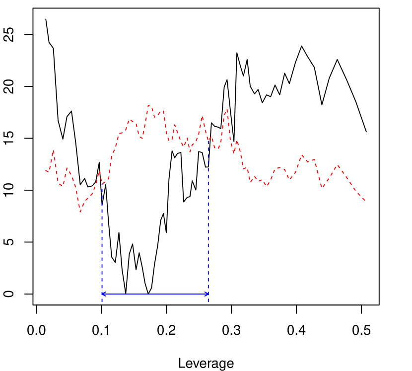
Subplot : a

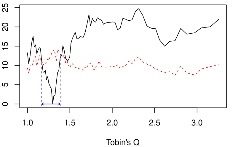
Subplot : b

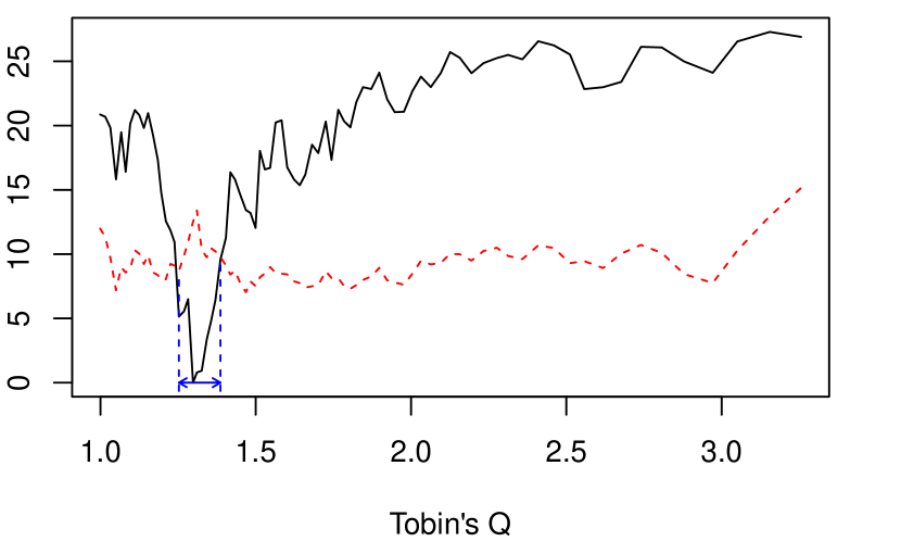
Subplot : c

7 Conclusion

This paper shows that the asymptotic distribution of the GMM estimator of the dynamic panel threshold models varies depending on whether the true models have a kink or a jump, and that the standard nonparametric bootstrap is inconsistent when the true model is the kink model. Therefore, alternative bootstrap methods are proposed for constructing the confidence sets of the coefficients and the threshold location and they are shown to be consistent independently to the continuity of the true model. The alternative bootstrap methods are shown to improve upon the standard nonparametric bootstrap and the asymptotic confidence intervals in the finite samples even when the model is discontinuous through Monte Carlo simulations.

There are further extensions of our work that we leave as future research, such as asymptotic analysis when the time series dimension grows, along with other features like some latent group structure or the interactive effect, as explored by Miao et al., 2020b , and Miao et al., 2020a , respectively. Extension of these works to the dynamic threshold model would be valuable. It is also left as a future research to check the uniform validity of the proposed bootstraps theoretically.

Additional Notations.

For $k,p\in\mathbb{N}$, $0_{k\times p}$ denotes $k\times p$ a matrix whose elements are all zero. “$\rightsquigarrow$” denotes the weak convergence as in section 1.3 of van der Vaart and Wellner, (1996). “$\lesssim$” means that the left side is bounded by a constant multiplied by the right side. $\|\cdot\|$ is a norm for either vectors or matrices. For a vector, it is the Euclidean norm. For a matrix, it is the Frobenius norm, i.e. $\|M\|=\sqrt{tr(M^{\prime}M)}$ for a matrix $M$.

Appendix A Proofs for Section 3.

A.1 Proof of Theorem 1.

The population moment equation is $g_{0}(\theta)=\left[\begin{array}[]{c;{2pt/2pt}c}M_{0}(\gamma)&M_{20}\delta_{0}\\ \end{array}\right]\times((\beta_{0}^{\prime}-\beta^{\prime},-\delta^{\prime}),1)^{\prime},$ when $\gamma\neq\gamma_{0}$, while $g_{0}(\theta)=M_{0}\times(\alpha-\alpha_{0})^{\prime}$ when $\gamma=\gamma_{0}$. Therefore, the conditions (i) and (ii) of Theorem 1 implies $g_{0}(\theta)\neq 0_{k}$ if $\theta\neq\theta_{0}$.

A.2 Proof of Theorem 2.

To obtain the limit distribution of $\hat{\theta}$, we first establish the consistency of $\hat{\theta}$ to $\theta_{0}$ and rate of $\hat{\theta}$’s convergence. Then we show the asymptotic distribution of the estimates using the rescaled versions of the parameters and criterions.

A.2.1 Consistency.

The constrained estimator of the coefficients, $\hat{\alpha}(\gamma)=\arg\min_{\alpha\in A}\hat{Q}_{n}(\alpha,\gamma)$, given a fixed $\gamma$ can be expressed as

$$\hat{\alpha}(\gamma)=-(\bar{M}_{n}(\gamma)^{\prime}W_{n}\bar{M}_{n}(\gamma))^{-1}\bar{M}_{n}(\gamma)^{\prime}W_{n}\bar{v}_{n}$$

where

$$\bar{v}_{n}=-\bar{M}_{n}\alpha_{0}+u_{n},\quad u_{n}=\frac{1}{n}\sum_{i=1}^{n}\begin{pmatrix}z_{it_{0}}\Delta\epsilon_{it_{0}}\\ \vdots\\ z_{iT}\Delta\epsilon_{iT}\end{pmatrix}.$$

Therefore,

$$\hat{\alpha}(\gamma)=-(\bar{M}_{n}(\gamma)^{\prime}W_{n}\bar{M}_{n}(\gamma))^{-1}\bar{M}_{n}(\gamma)^{\prime}W_{n}(-\bar{M}_{n}\alpha_{0}+u_{n}).$$

Define the profiled criterions with respect to $\gamma$ by $\tilde{g}_{n}(\gamma)=\bar{g}_{n}(\hat{\alpha}(\gamma),\gamma)$ and $\tilde{Q}_{n}(\gamma)=\tilde{g}_{n}(\gamma)^{\prime}W_{n}\tilde{g}_{n}(\gamma)$. The threshold location estimator is $\hat{\gamma}=\arg\min_{\gamma\in\Gamma}\tilde{g}_{n}(\gamma)^{\prime}W_{n}\tilde{g}_{n}(\gamma)$. By the law of large numbers (LLN), $u_{n}\xrightarrow{p}0$. By the uniform law of large numbers (ULLN) in Lemma 3, $\bar{M}_{n}(\gamma)\xrightarrow{p}M_{0}(\gamma)$ uniformly with respect to $\gamma\in\Gamma$. Hence, $\hat{\gamma}\xrightarrow{p}\gamma_{0}$ would imply $\bar{M}_{n}(\hat{\gamma})\xrightarrow{p}M_{0}$, and then $\hat{\alpha}(\hat{\gamma})\xrightarrow{p}\alpha_{0}$, which completes the proof.

To show the consistency of $\hat{\gamma}$ to $\gamma_{0}$, we apply the argmin/argmax continuous mapping theorem (CMT) as in Theorem 3.2.2 in van der Vaart and Wellner, (1996). It is sufficient to check (i) $\tilde{Q}_{n}(\gamma)$ uniformly converges to $\tilde{Q}_{0}(\gamma)$ in probability, and (ii) $\tilde{Q}_{0}(\gamma_{0})<\inf_{\gamma\not\in\mathcal{O}}\tilde{Q}_{0}(\gamma)$ for any open set $\mathcal{O}$ contatining $\gamma_{0}$. (ii) can be shown if $\tilde{Q}_{0}(\gamma)$ is uniquely minimized at $\gamma_{0}$ and continuous as $\Gamma$ is compact.

The profiled moment can be rewritten as

$$\tilde{g}_{n}(\gamma)=[I-\bar{M}_{n}(\gamma)\left(\bar{M}_{n}(\gamma)^{\prime}W_{n}\bar{M}_{n}(\gamma)\right)^{-1}\bar{M}_{n}(\gamma)^{\prime}W_{n}](-\bar{M}_{n}\alpha_{0}+u_{n}).$$

Therefore,

$$W_{n}^{1/2}\tilde{g}_{n}(\gamma)=[I-P_{W_{n}^{1/2}\bar{M}_{n}(\gamma)}](-W_{n}^{1/2}\bar{M}_{n}\alpha_{0}+W_{n}^{1/2}u_{n}),$$

where $P_{W_{n}^{1/2}\bar{M}_{n}(\gamma)}=W_{n}^{1/2}\bar{M}_{n}(\gamma)\left(\bar{M}_{n}(\gamma)^{\prime}W_{n}\bar{M}_{n}(\gamma)\right)^{-1}\bar{M}_{n}(\gamma)^{\prime}W_{n}^{1/2}$ is a projection matrix to the column space of $W_{n}^{1/2}\bar{M}_{n}(\gamma)$. The profiled objective can be written as

$$\tilde{Q}_{n}(\gamma)=\|(I-P_{W_{n}^{1/2}\bar{M}_{n}(\gamma)})(-W_{n}^{1/2}\bar{M}_{n}\alpha_{0}+W_{n}^{1/2}u_{n})\|^{2}.$$

By $W_{n}\xrightarrow{p}W$, $u_{n}\xrightarrow{p}0$, and $\sup_{\gamma\in\Gamma}\|\bar{M}_{n}(\gamma)-M_{0}(\gamma)\|\xrightarrow{p}0$, we can derive that

$$\tilde{Q}_{n}(\gamma)\xrightarrow{p}\tilde{Q}_{0}(\gamma)=\|(I-P_{W^{1/2}M_{0}(\gamma)})W^{1/2}M_{0}\alpha_{0}\|^{2}$$

uniformly with respect to $\gamma$, where $P_{W^{1/2}M_{0}(\gamma)}=W^{1/2}M_{0}(\gamma)\left(M_{0}(\gamma)^{\prime}WM_{0}(\gamma)\right)^{-1}M_{0}(\gamma)^{\prime}W^{1/2}$. Note that $W=\Omega^{-1}$ in the second stage of the two-step GMM estimation. $W=I$ when we consider the first stage. $\tilde{Q}_{0}(\gamma)$ is uniquely minimized when $\gamma=\gamma_{0}$. This is because $W$ is positive definite, and the conditions in Theorem 1 implies that $M_{0}\alpha_{0}$ does not lie in the column space of $M_{0}(\gamma)$ whenever $\gamma\neq\gamma_{0}$. Moreover, $\tilde{Q}_{0}(\gamma)$ is continuous as $M_{0}(\gamma)$ is continuous with respect to $\gamma$ by D.

A.2.2 Convergence rate.

Let us assume that $\|W_{n}-\Omega^{-1}\|\xrightarrow{p}0$ as the consistency of $\hat{\theta}_{0}$ is shown. Our proof follows the arguments similar to the proof of Theorem 3.3 by Pakes and Pollard, (1989). Let $\varepsilon_{n}(\theta)=\bar{g}_{n}(\theta)-\bar{g}_{n}(\theta_{0})-g_{0}(\theta)$. By Lemma 4, $\sup_{\|\theta-\theta_{0}\|<h_{n}}\sqrt{n}\|\varepsilon_{n}(\theta)\|=o_{p}(1)$ for any $h_{n}\downarrow 0$. Therefore, by the consistency of $\hat{\theta}$,

$$\sqrt{n}\|\bar{g}_{n}(\hat{\theta})-\bar{g}_{n}(\theta_{0})-g_{0}(\hat{\theta})\|=o_{p}(1).$$

By $\|W_{n}-\Omega^{-1}\|\xrightarrow{p}0$, we can obtain

$$\sqrt{n}\|W_{n}^{1/2}\bar{g}_{n}(\hat{\theta})-W_{n}^{1/2}\bar{g}_{n}(\theta_{0})-\Omega^{-1/2}g_{0}(\hat{\theta})\|=o_{p}(1).$$

Apply the triangle inequality to get

$$\sqrt{n}\|\Omega^{-1/2}g_{0}(\hat{\theta})\|\leq o_{p}(1)+\sqrt{n}\|W_{n}^{1/2}\bar{g}_{n}(\theta_{0})\|+\sqrt{n}\|W_{n}^{1/2}\bar{g}_{n}(\hat{\theta})\|.$$

As $\hat{\theta}$ is the minimizer of the GMM criterion, $\sqrt{n}\|W_{n}^{1/2}\bar{g}_{n}(\hat{\theta})\|\leq o_{p}(1)+\sqrt{n}\|W_{n}^{1/2}\bar{g}_{n}(\theta_{0})\|=O_{p}(1)$. Therefore,

$$\sqrt{n}\|\Omega^{-1/2}g_{0}(\hat{\theta})\|\leq O_{p}(1).$$

By Lemma 2, $\sqrt{n}\|\Omega^{-1/2}g_{0}(\hat{\theta})\|\geq C\sqrt{n}(\|\hat{\alpha}-\alpha_{0}\|+(\hat{\gamma}-\gamma_{0})^{2})$ for some constant $C\in(0,+\infty)$. Therefore,

$$\sqrt{n}(\|\hat{\alpha}-\alpha_{0}\|+(\hat{\gamma}-\gamma_{0})^{2})\leq O_{p}(1)$$

which implies $\|\hat{\alpha}-\alpha_{0}\|=O_{p}(n^{-1/2})$ and $(\hat{\gamma}-\gamma_{0})^{2}=O_{p}(n^{-1/2})$.

A.2.3 Asymptotic distribution.

This section derives an asymptotic distribution of the estimator through the argmin/argmax continuous mapping theorem (CMT) as in Theorem 3.2.2 in van der Vaart and Wellner, (1996).

Introduce a local reparametrization by $a=\sqrt{n}(\alpha-\alpha_{0})$ and $b=n^{\frac{1}{4}}(\gamma-\gamma_{0})$, and let $a$ consist of subvectors $a_{1}=\sqrt{n}(\beta-\beta_{0})$ and $a_{2}=\sqrt{n}(\delta-\delta_{0})$. Additionally define $\hat{a}=\sqrt{n}(\hat{\alpha}-\alpha_{0})$ and $\hat{b}=n^{\frac{1}{4}}(\hat{\gamma}-\gamma_{0})$. Let

$$\mathbb{S}_{n}(a,b)=n\hat{Q}_{n}(\alpha_{0}+\tfrac{a}{\sqrt{n}},\gamma_{0}+\tfrac{b}{n^{\frac{1}{4}}})=n\bar{g}_{n}(\alpha_{0}+\tfrac{a}{\sqrt{n}},\gamma_{0}+\tfrac{b}{n^{\frac{1}{4}}})^{\prime}W_{n}\bar{g}_{n}(\alpha_{0}+\tfrac{a}{\sqrt{n}},\gamma_{0}+\tfrac{b}{n^{\frac{1}{4}}}).$$

We show that (i) $\mathbb{S}_{n}$ weakly converges to a stochastic process $\mathbb{S}$ in $\ell^{\infty}(\mathbb{K})$ for every compact $\mathbb{K}$ in the Euclidean space, (ii) $\mathbb{S}$ is continuous, and (iii) $\mathbb{S}$ possesses unique optimums not in $b$ but in its square $b^{2}$ since $\mathbb{S}(a,b)=\mathbb{S}(a,-b)$. Thus, we will establish that $(\hat{a}^{\prime},\hat{b}^{2})^{\prime}$ converges in distribution to $(a_{0}^{\prime},b_{0}^{2})^{\prime}=\arg\min_{a,b^{2}}\mathbb{S}(a,\sqrt{b^{2}})$. In the characterization of the minimizers, $(a_{0}^{\prime},b_{0}^{2})^{\prime}$ is shown to be tight. Note that $(\hat{a},\hat{b}^{2})$ is uniformly tight due to the convergence rate we obtained.

The rescaled and reparametrized sample moment can be written as

$$\sqrt{n}\bar{g}_{n}(\alpha_{0}+\tfrac{a}{\sqrt{n}},\gamma_{0}+\tfrac{b}{n^{\frac{1}{4}}})= \sqrt{n}\begin{pmatrix}\frac{1}{n}\sum_{i=1}^{n}z_{it_{0}}\Delta\epsilon_{it_{0}}\\ \vdots\\ \frac{1}{n}\sum_{i=1}^{n}z_{iT}\Delta\epsilon_{iT}\end{pmatrix}-\begin{pmatrix}\tfrac{1}{n}\sum_{i=1}^{n}z_{it_{0}}\Delta x_{it_{0}}^{\prime}\\ \vdots\\ \tfrac{1}{n}\sum_{i=1}^{n}z_{iT}\Delta x_{iT}^{\prime}\end{pmatrix}a_{1}$$

$$-\begin{pmatrix}\tfrac{1}{n}\sum_{i=1}^{n}z_{it_{0}}1_{it_{0}}(\gamma_{0}+\tfrac{b}{n^{\frac{1}{4}}})^{\prime}X_{it_{0}}\\ \vdots\\ \tfrac{1}{n}\sum_{i=1}^{n}z_{iT}1_{iT}(\gamma_{0}+\tfrac{b}{n^{\frac{1}{4}}})^{\prime}X_{iT}\end{pmatrix}a_{2}$$

$$+\sqrt{n}\begin{pmatrix}\tfrac{1}{n}\sum_{i=1}^{n}z_{it_{0}}(1_{it_{0}}(\gamma_{0})^{\prime}-1_{it_{0}}(\gamma_{0}+\tfrac{b}{n^{\frac{1}{4}}})^{\prime})X_{it_{0}}\\ \vdots\\ \tfrac{1}{n}\sum_{i=1}^{n}z_{iT}(1_{iT}(\gamma_{0})^{\prime}-1_{iT}(\gamma_{0}+\tfrac{b}{n^{\frac{1}{4}}})^{\prime})X_{iT}\end{pmatrix}\delta_{0}.$$

By the central limit theorem (CLT),

$$\sqrt{n}\begin{pmatrix}\frac{1}{n}\sum_{i=1}^{n}z_{it_{0}}\Delta\epsilon_{it_{0}}\\ \vdots\\ \frac{1}{n}\sum_{i=1}^{n}z_{iT}\Delta\epsilon_{iT}\end{pmatrix}\xrightarrow{d}-e\sim N(0,\Omega).$$

By the LLN,

$$\begin{pmatrix}\tfrac{1}{n}\sum_{i=1}^{n}z_{it_{0}}\Delta x_{it_{0}}^{\prime}\\ \vdots\\ \tfrac{1}{n}\sum_{i=1}^{n}z_{iT}\Delta x_{iT}^{\prime}\end{pmatrix}\xrightarrow{p}\begin{pmatrix}Ez_{it_{0}}\Delta x_{it_{0}}^{\prime}\\ \vdots\\ Ez_{iT}\Delta x_{iT}^{\prime}\end{pmatrix}$$

Let $K<\infty$ be arbitrary. By the ULLN in Lemma 3,

$$\left\|\begin{pmatrix}\tfrac{1}{n}\sum_{i=1}^{n}z_{it_{0}}1_{it_{0}}(\gamma_{0}+\tfrac{b}{n^{\frac{1}{4}}})^{\prime}X_{it_{0}}\\ \vdots\\ \tfrac{1}{n}\sum_{i=1}^{n}z_{iT}1_{iT}(\gamma_{0}+\tfrac{b}{n^{\frac{1}{4}}})^{\prime}X_{iT}\end{pmatrix}-\begin{pmatrix}Ez_{it_{0}}1_{it_{0}}(\gamma_{0}+\tfrac{b}{n^{\frac{1}{4}}})^{\prime}X_{it_{0}}\\ \vdots\\ Ez_{iT}1_{iT}(\gamma_{0}+\tfrac{b}{n^{\frac{1}{4}}})^{\prime}X_{iT}\end{pmatrix}\right\|\xrightarrow{p}0$$

uniformly with respect to $b\in[-K,K]$. Then by the continuity of $\kappa\mapsto E[z_{it}1_{it}(\gamma+\kappa)X_{it}]$ at $\kappa=0$,

$$\begin{pmatrix}\tfrac{1}{n}\sum_{i=1}^{n}z_{it_{0}}1_{it_{0}}(\gamma_{0}+\tfrac{b}{n^{\frac{1}{4}}})^{\prime}X_{it_{0}}\\ \vdots\\ \tfrac{1}{n}\sum_{i=1}^{n}z_{iT}1_{iT}(\gamma_{0}+\tfrac{b}{n^{\frac{1}{4}}})^{\prime}X_{iT}\end{pmatrix}\xrightarrow{p}\begin{pmatrix}Ez_{it_{0}}1_{it_{0}}(\gamma_{0})^{\prime}X_{it_{0}}\\ \vdots\\ Ez_{iT}1_{iT}(\gamma_{0})^{\prime}X_{iT}\end{pmatrix}$$

uniformly with respect to $b\in[-K,K]$. By Lemma 5,

$$\sqrt{n}\begin{pmatrix}\tfrac{1}{n}\sum_{i=1}^{n}z_{it_{0}}(1_{it_{0}}(\gamma_{0})^{\prime}-1_{it_{0}}(\gamma_{0}+\tfrac{b}{n^{\frac{1}{4}}})^{\prime})X_{it_{0}}\delta_{0}\\ \vdots\\ \tfrac{1}{n}\sum_{i=1}^{n}z_{iT}(1_{iT}(\gamma_{0})^{\prime}-1_{iT}(\gamma_{0}+\tfrac{b}{n^{\frac{1}{4}}})^{\prime})X_{iT}\delta_{0}\end{pmatrix}\xrightarrow{p}\frac{\delta_{30}}{2}\begin{pmatrix}E_{t_{0}}[z_{it_{0}}|\gamma_{0}]f_{t_{0}}(\gamma_{0})-E_{t_{0}-1}[z_{iT}|\gamma_{0}]f_{t_{0}-1}(\gamma_{0})\\ \vdots\\ E_{T}[z_{iT}|\gamma_{0}]f_{T}(\gamma_{0})-E_{T-1}[z_{iT}|\gamma_{0}]f_{T-1}(\gamma_{0})\end{pmatrix}b^{2}$$

uniformly with respect to $b\in[-K,K]$.

Therefore, $\mathbb{S}_{n}(a,b)$ weakly converges to

$$\mathbb{S}(a,b)=(M_{0}a+Hb^{2}-e)^{\prime}\Omega^{-1}(M_{0}a+Hb^{2}-e),$$

in $\ell^{\infty}(\mathbb{K})$ for any compact $\mathbb{K}\subset\mathbb{R}^{2p+2}$. Then by the CMT,

$$(\hat{a},\hat{b}^{2})\xrightarrow{d}\arg\min_{a,b^{2}}(M_{0}a+Hb^{2}-e)^{\prime}\Omega^{-1}(M_{0}a+Hb^{2}-e).$$

Characterization of the minimizers

Next, we characterize the minimizers. The objective function of the minimization problem is strictly convex with respect to $a$ and $b^{2}$, since $\left[\begin{array}[]{c;{2pt/2pt}c}M_{0}&H\end{array}\right]$ has full column rank and $\Omega^{-1}$ is positive definite. Hence, a solution $(a_{0}^{\prime},b_{0}^{2})^{\prime}$ can be characterized by the Karush-Kuhn-Tucker conditions. See Chapter 5 in Boyd and Vandenberghe, (2004) for more details.

The Lagrangian for this problem is

$$\mathcal{L}(a,b,\lambda)=a^{\prime}M_{0}^{\prime}\Omega^{-1}M_{0}a+2a^{\prime}M_{0}^{\prime}\Omega^{-1}Hb^{2}+H^{\prime}\Omega^{-1}Hb^{4}-2a^{\prime}M_{0}^{\prime}\Omega^{-1}e-2H^{\prime}\Omega^{-1}e\cdot b^{2}+e^{\prime}\Omega^{-1}e-\lambda b^{2}$$

and the gradient of the Lagrangian with respect to $a$ and $b^{2}$ should vanish:

$$a: \quad M_{0}^{\prime}\Omega^{-1}M_{0}a+M_{0}^{\prime}\Omega^{-1}Hb^{2}-M_{0}^{\prime}\Omega^{-1}e=0$$

$$b^{2}: \quad H^{\prime}\Omega^{-1}Hb^{2}+H^{\prime}\Omega^{-1}M_{0}a-H^{\prime}\Omega^{-1}e-\lambda=0.$$

In addition, $\lambda\geq 0$ and $\lambda b^{2}=0$ should hold.

1. When $\lambda=0$ and $b^{2}\geq 0$, we can obtain

   $$b^{2}=(H^{\prime}\Omega^{-1/2}(I-P_{\Omega^{-1/2}M_{0}})\Omega^{-1/2}H)^{-1}H^{\prime}\Omega^{-1/2}(I-P_{\Omega^{-1/2}M_{0}})\Omega^{-1/2}e,$$

   where $P_{\Omega^{-1/2}M_{0}}=\Omega^{-1/2}M_{0}(M_{0}^{\prime}\Omega^{-1}M_{0})^{-1}M_{0}^{\prime}\Omega^{-1/2}$ is the projection matrix to the column space of $\Omega^{-1/2}M_{0}$. $H^{\prime}\Omega^{-1/2}(I-P_{\Omega^{-1/2}M_{0}})\Omega^{-1/2}H>0$ because the matrix $\left[\begin{array}[]{c;{2pt/2pt}c}M_{0}&H\end{array}\right]$ has full column rank, and $\Omega^{-1/2}H$ cannot be in the column space of $\Omega^{-1/2}M_{0}$ and $(I-P_{\Omega^{-1/2}M_{0}})\Omega^{-1/2}H\neq 0$. Therefore,

   $$H^{\prime}\Omega^{-1/2}(I-P_{\Omega^{-1/2}M_{0}})\Omega^{-1/2}e\geq 0$$

   should hold for the feasibility condition $b^{2}\geq 0$.

2. When $\lambda>0$ and $b^{2}=0$, we can obtain

   $$a=(M_{0}^{\prime}\Omega^{-1}M_{0})^{-1}M_{0}^{\prime}\Omega^{-1}e.$$

   By plugging this into the equation for $b^{2}$, we get

   $$H^{\prime}\Omega^{-1/2}(I-P_{\Omega^{-1/2}M_{0}})\Omega^{-1/2}e<0.$$

Thus,

$$b_{0}^{2}=\begin{cases}[H^{\prime}\Xi H]^{-1}H^{\prime}\Xi e&\text{if }H^{\prime}\Xi e\geq 0\\ \quad\quad 0&\text{else}\\ \end{cases}$$

where $\Xi=\Omega^{-1/2}(I-P_{\Omega^{-1/2}M_{0}})\Omega^{-1/2}$. $b_{0}^{2}$ follows a normal distribution that is left censored at 0. Then

$$a_{0}=\begin{cases}(M_{0}^{\prime}\Omega^{-1}M_{0})^{-1}M_{0}^{\prime}\Omega^{-1}[I-H[H^{\prime}\Xi H]^{-1}H^{\prime}\Xi]e&\text{if }H^{\prime}\Xi e\geq 0\\ (M_{0}^{\prime}\Omega^{-1}M_{0})^{-1}M_{0}^{\prime}\Omega^{-1}e&\text{else.}\end{cases}$$

Note that the two normal variables $(M_{0}^{\prime}\Omega^{-1}M_{0})^{-1}M_{0}^{\prime}\Omega^{-1}H[H^{\prime}\Xi H]^{-1}H^{\prime}\Xi e$ and $(M_{0}^{\prime}\Omega^{-1}M_{0})^{-1}M_{0}^{\prime}\Omega^{-1}e$ are independent of each other, because $E[H^{\prime}\Xi ee^{\prime}\Omega^{-1}M_{0}]=H^{\prime}\Omega^{-1/2}(I-P_{\Omega^{-1/2}M_{0}})\Omega^{-1/2}M_{0}$ becomes zero.

Appendix B Proofs for Section 4

B.1 Preliminaries

The bootstrap methods we consider are Algorithm 1 with different choices of $\theta_{0}^{*}$. There are three bootstrap methods this paper propose: (i) $\theta_{0}^{*}$ set as (10), (ii) $\theta_{0}^{*}=(\hat{\alpha}(\gamma),\gamma)^{\prime}$ for $\gamma\in\Gamma$, and (iii) $\theta_{0}^{*}=\tilde{\theta}$ which is the continuity restricted estimator. In Appendix C, we consider the case $\theta_{0}^{*}=\hat{\theta}$.

The probability law for the bootstrap is formalized following Goncalves and White, (2004). Let $P$ be the probability measure for data and $P^{*}$ be the conditional probability law of bootstrap given observations. $Z_{n}^{*}\xrightarrow{p^{*}}0$ in $P$ ($Z_{n}^{*}=o_{p}^{*}(1)$ in $P$) if for any $\epsilon,\delta>0$, $P(P^{*}(|Z_{n}^{*}|>\epsilon)>\delta)\rightarrow 0$ as $n\rightarrow\infty$. $Z_{n}^{*}=O_{p}^{*}(1)$ in $P$ if for any $\delta>0$, there exists $M<\infty$ such that $P(P^{*}(|Z_{n}^{*}|\geq M)>\delta)\rightarrow 0$ as $n\rightarrow\infty$. $Z_{n}^{*}\xrightarrow{d^{*}}Z$ in $P$ if $E^{*}f(Z_{n}^{*})\rightarrow Ef(Z)$ in $P$ for every continuous and bounded function $f$, where $E^{*}$ is the expectation by the bootstrap probability law conditional on observations. $Z_{n}^{*}\overset{*}{\rightsquigarrow}Z$ in $\ell^{\infty}(\mathbb{K})$ in $P$ if $\sup_{f\in BL_{1}}|E^{*}f(Z_{n}^{*})-Ef(Z_{n})|\xrightarrow{p}0$, where $BL_{1}$ is the set of all Lipschitz functions on $\ell^{\infty}(\mathbb{K})$ bounded in $[0,1]$ such that $|f(z_{1})-f(z_{2})|\leq\|z_{1}-z_{2}\|_{\ell^{\infty}(\mathbb{K})}=\sup_{x\in\mathbb{K}}|z_{1}(x)-z_{2}(x)|$.

The following lemma is useful in analyzing bootstrap stochastic orders.

Lemma 1.

1. If $A_{n}=o_{p}(1)$ or $O_{p}(1)$, then $A_{n}=o_{p}^{*}(1)$ or $O_{p}^{*}(1)$ in $P$, respectively.

2. Let $Z_{n}^{*}=o_{p}^{*}(1)$ in $P$ and $W_{n}^{*}=O_{p}^{*}(1)$ in $P$. Then, $Z_{n}^{*}\times W_{n}^{*}=o_{p}^{*}(1)$ in $P$.

Proof.

See Lemma 3 in Cheng and Huang, (2010). ∎

Recall that $W_{n}^{*}=\{[\frac{1}{n}\sum_{i=1}^{n}g_{i}^{*}(\hat{\theta}_{0})g_{i}^{*}(\hat{\theta}_{0})^{\prime}]-[\frac{1}{n}\sum_{i=1}^{n}g_{i}^{*}(\theta)][\frac{1}{n}\sum_{i=1}^{n}g_{i}^{*}(\theta)^{\prime}]\}^{-1}$. $\|W_{n}^{*}-\Omega^{-1}\|=o_{p}^{*}(1)$ in $P$ when $\hat{\theta}_{0}^{*}\xrightarrow{p^{*}}\theta_{0}$ in $P$. This would be the case when $\hat{\theta}_{0}^{*}\xrightarrow{p^{*}}\theta_{0}^{*}$ in $P$ and $\|\theta_{0}^{*}-\theta_{0}\|=o_{p}(1)$ since then $\|\hat{\theta}_{0}^{*}-\theta_{0}\|\leq\|\hat{\theta}_{0}^{*}-\theta_{0}^{*}\|+\|\theta_{0}^{*}-\theta_{0}\|=o_{p}^{*}(1)$ in $P$ by Lemma 1.

B.2 Proof of Theorem 5.

As in the proof of Theorem 2, the consistency and convergence rate of the bootstrap estimator is derived first. Then we derive the (conditional) weak convergence limit of the rescaled criterion and apply the CMT to obtain the asymptotic distribution of the bootstrap estimator. Recall that $\theta_{0}^{*}$ is set as (10) in Theorem 5. For both cases (i) and (ii) of the theorem, $\theta_{0}^{*}\xrightarrow{p}\theta_{0}$ which implies $\theta_{0}^{*}\xrightarrow{p^{*}}\theta_{0}$ in $P$ by Lemma 1.

Consistency of the bootstrap estimator.

The bootstrap sample moment can be rewritten by

$$\bar{g}_{n}^{*}(\theta) =\frac{1}{n}\sum_{i=1}^{n}(g_{i}^{*}(\theta)-\bar{g}_{n}(\hat{\theta}))$$

$$=\begin{pmatrix}\frac{1}{n}\sum_{i=1}^{n}z_{it_{0}}^{*}\widehat{\Delta\epsilon}_{it_{0}}^{*}\\ \vdots\\ \frac{1}{n}\sum_{i=1}^{n}z_{iT}^{*}\widehat{\Delta\epsilon}_{iT}^{*}\end{pmatrix}-\begin{pmatrix}\frac{1}{n}\sum_{i=1}^{n}z_{it_{0}}\widehat{\Delta\epsilon}_{it_{0}}\\ \vdots\\ \frac{1}{n}\sum_{i=1}^{n}z_{iT}\widehat{\Delta\epsilon}_{iT}\end{pmatrix}$$

$$-\begin{pmatrix}\frac{1}{n}\sum_{i=1}^{n}z_{it_{0}}^{*}\Delta x_{it_{0}}^{*\prime}\\ \vdots\\ \frac{1}{n}\sum_{i=1}^{n}z_{iT}^{*}\Delta x_{iT}^{*\prime}\end{pmatrix}(\beta-\beta_{0}^{*})-\begin{pmatrix}\frac{1}{n}\sum_{i=1}^{n}z_{it_{0}}^{*}1_{it_{0}}^{*}(\gamma)^{\prime}X_{it_{0}}^{*}\\ \vdots\\ \frac{1}{n}\sum_{i=1}^{n}z_{iT}^{*}1_{iT}^{*}(\gamma)^{\prime}X_{iT}^{*}\end{pmatrix}(\delta-\delta_{0}^{*})$$

$$+\begin{pmatrix}\frac{1}{n}\sum_{i=1}^{n}z_{it_{0}}^{*}(1_{it_{0}}^{*}(\gamma_{0}^{*})-1_{it_{0}}^{*}(\gamma))^{\prime}X_{it_{0}}^{*}\\ \vdots\\ \frac{1}{n}\sum_{i=1}^{n}z_{iT}^{*}(1_{iT}^{*}(\gamma_{0}^{*})-1_{iT}^{*}(\gamma))^{\prime}X_{iT}^{*}\end{pmatrix}\delta_{0}^{*}.$$

We additionally define

$$v_{i}^{*}= \begin{pmatrix}z_{it_{0}}^{*}\Delta y_{it_{0}}^{*}\\ \vdots\\ z_{iT}^{*}\Delta y_{iT}^{*}\end{pmatrix}-\begin{pmatrix}\frac{1}{n}\sum_{i=1}^{n}z_{it_{0}}\widehat{\Delta\epsilon}_{it_{0}}\\ \vdots\\ \frac{1}{n}\sum_{i=1}^{n}z_{iT}\widehat{\Delta\epsilon}_{iT}\end{pmatrix} ,\quad M_{i}^{*}(\gamma)= -\begin{bmatrix}z_{it_{0}^{*}}(\Delta x_{it_{0}}^{*\prime},1_{it_{0}}^{*}(\gamma)^{\prime}X_{it_{0}}^{*})\\ \vdots\\ z_{iT}^{*}(\Delta x_{iT}^{*\prime},1_{iT}^{*}(\gamma)^{\prime}X_{iT}^{*})\end{bmatrix},$$

$\bar{v}_{n}^{*}=\frac{1}{n}\sum_{i=1}^{n}v_{i}^{*}$, and $\bar{M}_{n}^{*}(\gamma)=\frac{1}{n}\sum_{i=1}^{n}M_{i}^{*}(\gamma)$. Then $\bar{g}_{n}^{*}(\theta)=\bar{v}_{n}^{*}+\bar{M}_{n}^{*}(\gamma)\alpha$. Given $\gamma$, we can obtain the constrained optimizer

$$\hat{\alpha}^{*}(\gamma)=-(\bar{M}_{n}^{*\prime}(\gamma)W_{n}^{*}\bar{M}_{n}^{*}(\gamma))^{-1}\bar{M}_{n}^{*\prime}(\gamma)W_{n}^{*}\bar{v}_{n}^{*}$$

where

$$\bar{v}_{n}^{*}=-\bar{M}_{n}^{*}(\gamma_{0}^{*})\alpha_{0}^{*}+\hat{u}_{n}^{*};\quad\hat{u}_{n}^{*}=\begin{pmatrix}\frac{1}{n}\sum_{i=1}^{n}z_{it_{0}}^{*}\widehat{\Delta\epsilon}_{it_{0}}^{*}\\ \vdots\\ \frac{1}{n}\sum_{i=1}^{n}z_{iT}^{*}\widehat{\Delta\epsilon}_{iT}^{*}\end{pmatrix}-\begin{pmatrix}\frac{1}{n}\sum_{i=1}^{n}z_{it_{0}}\widehat{\Delta\epsilon}_{it_{0}}\\ \vdots\\ \frac{1}{n}\sum_{i=1}^{n}z_{iT}\widehat{\Delta\epsilon}_{iT}\end{pmatrix}.$$

Let $\tilde{Q}_{n}^{*}(\gamma)=\hat{Q}_{n}^{*}(\hat{\alpha}^{*}(\gamma),\gamma)$ be a profiled criterion and $\hat{\gamma}^{*}=\arg\min_{\gamma\in\Gamma}\tilde{Q}_{n}^{*}(\gamma)$. $\hat{u}_{n}^{*}=o_{p}^{*}(1)$ in $P$ by Lemma 6. $\{M_{i}(\gamma):\gamma\in\Gamma\}$ is shown to be a Glivenko-Cantelli class in the proof of Lemma 3. By the bootstrap Glivenko-Cantelli (e.g. Lemma 3.6.16 in van der Vaart and Wellner, (1996)), $\sup_{\gamma\in\Gamma}\|\bar{M}_{n}^{*}(\gamma)-M_{0}(\gamma)\|=o_{p}^{*}(1)$ in $P$. Therefore, if $\hat{\gamma}^{*}\xrightarrow{p^{*}}\gamma_{0}^{*}$ in $P$, then $\hat{\alpha}^{*}=\hat{\alpha}^{*}(\hat{\gamma}^{*})\xrightarrow{p^{*}}\alpha_{0}^{*}$ in $P$, which completes the proof.

Let $\tilde{g}_{n}^{*}(\gamma)=\bar{g}_{n}^{*}(\hat{\alpha}^{*}(\gamma),\gamma)$ which can be expressed as

$$\tilde{g}_{n}^{*}(\gamma)=\left[I-\bar{M}_{n}^{*}(\gamma)(\bar{M}_{n}^{*\prime}(\gamma)W_{n}^{*}\bar{M}_{n}^{*}(\gamma))^{-1}\bar{M}_{n}^{*\prime}(\gamma)W_{n}^{*}\right]\left(-\bar{M}_{n}^{*}(\gamma_{0}^{*})\alpha_{0}^{*}+\hat{u}_{n}^{*}\right).$$

Therefore,

$$W_{n}^{*1/2}\tilde{g}_{n}^{*}(\gamma)=\left[I-P_{W_{n}^{*1/2}\bar{M}_{n}^{*}(\gamma)}\right]\left(-W_{n}^{*1/2}\bar{M}_{n}^{*}(\gamma_{0}^{*})\alpha_{0}^{*}+W_{n}^{*1/2}\hat{u}_{n}^{*}\right),$$

and

$$\sup_{\gamma\in\Gamma}\left|\tilde{Q}_{n}^{*}(\gamma)-\left\|\left[I-P_{W^{1/2}M_{0}(\gamma)}\right]\left(-W^{1/2}M_{0}(\gamma_{0})\alpha_{0}\right)\right\|^{2}\right|=o_{p}^{*}(1)\text{ in $P$}$$

when $\|W_{n}^{*}-W\|=o_{p}^{*}(1)$ in $P$ and $\theta_{0}^{*}\xrightarrow{p}\theta_{0}$. Note that $W$ is the identity matrix if it is for the first step estimation and $\Omega^{-1}$ if it is for the second step estimation if the first step estimator is consistent. Since the uniform conditional probability limit of $\tilde{Q}_{n}^{*}(\gamma)$ is minimized when $\gamma=\gamma_{0}$, the argmin CMT implies $\hat{\gamma}^{*}-\gamma_{0}=o_{p}^{*}(1)$ in $P$. As $\gamma_{0}^{*}-\gamma_{0}=o_{p}^{*}(1)$ in $P$ by Lemma 1, we can derive that $\hat{\gamma}^{*}-\gamma_{0}^{*}=o_{p}^{*}(1)$ in $P$.

Convergence rate under continuity.

As $\hat{\theta}^{*}$ is consistent to $\theta_{0}^{*}$ and $\theta_{0}^{*}\xrightarrow{p^{*}}\theta_{0}$ in $P$ by Lemma 1, we consider $\hat{\theta}^{*}$ and $\theta_{0}^{*}$ in a neighborhood of $\theta_{0}$. Let $\varepsilon_{n}^{*}(\theta)=\bar{g}_{n}^{*}(\theta)-\bar{g}_{n}^{*}(\theta_{0})-\bar{g}_{n}(\theta)+\bar{g}_{n}(\theta_{0})$. By the bootstrap equicontinuity, Lemma 8, $\sqrt{n}\|\varepsilon_{n}^{*}(\hat{\theta}^{*})\|=o_{p}^{*}(1)$ in $P$ and $\sqrt{n}\|\varepsilon_{n}^{*}(\theta_{0}^{*})\|=o_{p}^{*}(1)$ in $P$. Therefore,

$$\sqrt{n}\|\bar{g}_{n}^{*}(\hat{\theta}^{*})-\bar{g}_{n}^{*}(\theta_{0}^{*})-\bar{g}_{n}(\hat{\theta}^{*})+\bar{g}_{n}(\theta_{0}^{*})\|=o_{p}^{*}(1)\text{ in $P$.}$$

$\|W_{n}^{*}-W_{n}\|\xrightarrow{p^{*}}0$ in $P$ since $\|W_{n}^{*}-\Omega^{-1}\|=o_{p}^{*}(1)$. This is implied by $\hat{\theta}_{0}^{*}\xrightarrow{p^{*}}\theta_{0}$ in $P$, and $\|W_{n}-\Omega^{-1}\|=o_{p}^{*}(1)$ in $P$ by Lemma 1. Then

$$\sqrt{n}\|W_{n}^{*1/2}\bar{g}_{n}^{*}(\hat{\theta}^{*})-W_{n}^{*1/2}\bar{g}_{n}^{*}(\theta_{0}^{*})-W_{n}^{1/2}\bar{g}_{n}(\hat{\theta}^{*})+W_{n}^{1/2}\bar{g}_{n}(\theta_{0}^{*})\|=o_{p}^{*}(1)\text{ in $P$}.$$

Apply the triangle inequality to get

$$\sqrt{n}\|W_{n}^{1/2}\bar{g}_{n}(\hat{\theta}^{*})-W_{n}^{1/2}\bar{g}_{n}(\theta_{0}^{*})\|\leq o_{p}^{*}(1)+\sqrt{n}\|W_{n}^{*1/2}\bar{g}_{n}^{*}(\theta_{0}^{*})\|+\sqrt{n}\|W_{n}^{*1/2}\bar{g}_{n}^{*}(\hat{\theta}^{*})\|$$

where $o_{p}^{*}(1)$ holds in $P$. As $\hat{\theta}^{*}$ is the minimizer of the bootstrap criterion, $\sqrt{n}\|W_{n}^{*1/2}\bar{g}_{n}^{*}(\hat{\theta}^{*})\|\leq o_{p}^{*}(1)+\sqrt{n}\|W_{n}^{*1/2}\bar{g}_{n}^{*}(\theta_{0}^{*})\|=O_{p}^{*}(1)$ in $P$ where the last equality is implied by Lemma 7. Therefore,

$$\sqrt{n}\|W_{n}^{1/2}\bar{g}_{n}(\hat{\theta}^{*})-W_{n}^{1/2}\bar{g}_{n}(\theta_{0}^{*})\|\leq O_{p}^{*}(1)\text{ in $P$}.$$

By Lemma 4, $\sqrt{n}\|W_{n}^{1/2}\bar{g}_{n}(\hat{\theta}^{*})-W_{n}^{1/2}\bar{g}_{n}(\theta_{0}^{*})-\Omega^{-1/2}g_{0}(\hat{\theta}^{*})+\Omega^{-1/2}g_{0}(\theta_{0}^{*})\|=o_{p}(1)$, so it is $o_{p}^{*}(1)$ in $P$ by Lemma 1. Hence,

$$\sqrt{n}\|\Omega^{-1/2}g_{0}(\hat{\theta}^{*})-\Omega^{-1/2}g_{0}(\theta_{0}^{*})\|\leq O_{p}^{*}(1)\text{ in $P$}.$$

By Lemma 2, $\sqrt{n}\|\Omega^{-1/2}g_{0}(\hat{\theta}^{*})-\Omega^{-1/2}g_{0}(\theta_{0}^{*})\|=\sqrt{n}\|\Omega^{-1/2}M_{0}(\hat{\alpha}^{*}-\alpha_{0}^{*})+\Omega^{-1/2}H\{(\hat{\gamma}^{*}-\gamma_{0})^{2}-(\gamma_{0}^{*}-\gamma_{0})^{2}\}\|+o(\|\hat{\alpha}^{*}-\alpha_{0}^{*}\|+(\hat{\gamma}^{*}-\gamma_{0})^{2}+(\gamma_{0}^{*}-\gamma_{0})^{2})$. If $\sqrt{n}(\gamma_{0}^{*}-\gamma_{0})^{2}=O_{p}(1)$, then it is $O_{p}^{*}(1)$ in $P$ by Lemma 1. This is true for $\gamma_{0}^{*}=\hat{\gamma}$. Therefore, $\sqrt{n}\|\hat{\alpha}^{*}-\alpha_{0}^{*}\|=O_{p}^{*}(1)$ in $P$ and $\sqrt{n}(\hat{\gamma}^{*}-\gamma_{0})^{2}=O_{p}^{*}(1)$ in $P$. Then $\sqrt{n}(\hat{\gamma}^{*}-\gamma_{0}^{*})^{2}=O_{p}^{*}(1)$ in $P$ since $\sqrt{n}(\hat{\gamma}^{*}-\gamma_{0}^{*})^{2}\leq 2\sqrt{n}[(\hat{\gamma}^{*}-\gamma_{0})^{2}+(\gamma_{0}^{*}-\gamma_{0})^{2}]=O_{p}^{*}(1)$ in $P$.

Asymptotic distribution under continuity.

Introduce the local reparametrization by $a=\sqrt{n}(\alpha-\alpha_{0}^{*})$ and $b=n^{\frac{1}{4}}(\gamma-\gamma_{0}^{*})$, and let $a$ consist of subvectors $a_{1}=\sqrt{n}(\beta-\beta_{0}^{*})$ and $a_{2}=\sqrt{n}(\delta-\delta_{0}^{*})$.

The asymptotic distributions of the bootstrap estimators can be derived by using the argmin/argmax CMT as in the proof of Theorem 2. Let

$$\mathbb{S}_{n}^{*}(a,b)=n\hat{Q}_{n}^{*}(\alpha_{0}^{*}+\tfrac{a}{\sqrt{n}},\gamma_{0}^{*}+\tfrac{b}{n^{\frac{1}{4}}})=n\bar{g}_{n}^{*}(\alpha_{0}^{*}+\tfrac{a}{\sqrt{n}},\gamma_{0}^{*}+\tfrac{b}{n^{\frac{1}{4}}})^{\prime}W_{n}^{*}\bar{g}_{n}^{*}(\alpha_{0}^{*}+\tfrac{a}{\sqrt{n}},\gamma_{0}^{*}+\tfrac{b}{n^{\frac{1}{4}}}).$$

We show that $\mathbb{S}_{n}^{*}\overset{*}{\rightsquigarrow}\mathbb{S}$ in $\ell^{\infty}(\mathbb{K})$ in $P$ for every compact $\mathbb{K}$ in the Euclidean space. Recall that $\mathbb{S}(a,b)=(M_{0}a+Hb^{2}-e)^{\prime}\Omega^{-1}(M_{0}a+Hb^{2}-e)$.

The rescaled and reparametrized bootstrap moment can be written as

$$\sqrt{n}\bar{g}_{n}^{*}(\alpha_{0}^{*}+\tfrac{a}{\sqrt{n}},\gamma_{0}^{*}+\tfrac{b}{n^{\frac{1}{4}}})= \sqrt{n}\left\{\begin{pmatrix}\frac{1}{n}\sum_{i=1}^{n}z_{it_{0}}^{*}\widehat{\Delta\epsilon}_{it_{0}}^{*}\\ \vdots\\ \frac{1}{n}\sum_{i=1}^{n}z_{iT}^{*}\widehat{\Delta\epsilon}_{iT}^{*}\end{pmatrix}-\begin{pmatrix}\frac{1}{n}\sum_{i=1}^{n}z_{it_{0}}\widehat{\Delta\epsilon}_{it_{0}}\\ \vdots\\ \frac{1}{n}\sum_{i=1}^{n}z_{iT}\widehat{\Delta\epsilon}_{iT}\end{pmatrix}\right\}$$

$$-\begin{pmatrix}\tfrac{1}{n}\sum_{i=1}^{n}z_{it_{0}}^{*}\Delta x_{it_{0}}^{*\prime}\\ \vdots\\ \tfrac{1}{n}\sum_{i=1}^{n}z_{iT}^{*}\Delta x_{iT}^{*\prime}\end{pmatrix}a_{1}$$

$$-\begin{pmatrix}\tfrac{1}{n}\sum_{i=1}^{n}z_{it_{0}}^{*}1_{it_{0}}^{*}(\gamma_{0}^{*}+\tfrac{b}{n^{\frac{1}{4}}})^{\prime}X_{it_{0}}^{*}\\ \vdots\\ \tfrac{1}{n}\sum_{i=1}^{n}z_{iT}^{*}1_{iT}^{*}(\gamma_{0}^{*}+\tfrac{b}{n^{\frac{1}{4}}})^{\prime}X_{iT}^{*}\end{pmatrix}a_{2}$$

$$+\sqrt{n}\begin{pmatrix}\tfrac{1}{n}\sum_{i=1}^{n}z_{it_{0}}^{*}(1_{it_{0}}^{*}(\gamma_{0}^{*})^{\prime}-1_{it_{0}}(\gamma_{0}^{*}+\tfrac{b}{n^{\frac{1}{4}}})^{\prime})X_{it_{0}}^{*}\\ \vdots\\ \tfrac{1}{n}\sum_{i=1}^{n}z_{iT}^{*}(1_{iT}^{*}(\gamma_{0}^{*})^{\prime}-1_{iT}(\gamma_{0}^{*}+\tfrac{b}{n^{\frac{1}{4}}})^{\prime})X_{iT}^{*}\end{pmatrix}\delta_{0}^{*}.$$

By Lemma 7,

$$\sqrt{n}\left\{\begin{pmatrix}\frac{1}{n}\sum_{i=1}^{n}z_{it_{0}}^{*}\widehat{\Delta\epsilon}_{it_{0}}^{*}\\ \vdots\\ \frac{1}{n}\sum_{i=1}^{n}z_{iT}^{*}\widehat{\Delta\epsilon}_{iT}^{*}\end{pmatrix}-\begin{pmatrix}\frac{1}{n}\sum_{i=1}^{n}z_{it_{0}}\widehat{\Delta\epsilon}_{it_{0}}\\ \vdots\\ \frac{1}{n}\sum_{i=1}^{n}z_{iT}\widehat{\Delta\epsilon}_{iT}\end{pmatrix}\right\}\xrightarrow{d^{*}}-e\sim N(0,\Omega)\quad\text{ in $P$.}$$

By the bootstrap LLN,

$$\begin{pmatrix}\tfrac{1}{n}\sum_{i=1}^{n}z_{it_{0}}^{*}\Delta x_{it_{0}}^{*\prime}\\ \vdots\\ \tfrac{1}{n}\sum_{i=1}^{n}z_{iT}^{*}\Delta x_{iT}^{*\prime}\end{pmatrix}\xrightarrow{p^{*}}\begin{pmatrix}Ez_{it_{0}}\Delta x_{it_{0}}^{\prime}\\ \vdots\\ Ez_{iT}\Delta x_{iT}^{\prime}\end{pmatrix}\quad\text{ in $P$.}$$

Let $K<\infty$ be arbitrary. By the bootstrap Glivenko-Cantelli,

$$\sup_{b:|b|\leq K}\left\|\begin{pmatrix}\tfrac{1}{n}\sum_{i=1}^{n}z_{it_{0}}^{*}1_{it_{0}}^{*}(\gamma_{0}^{*}+\tfrac{b}{n^{\frac{1}{4}}})^{\prime}X_{it_{0}}^{*}\\ \vdots\\ \tfrac{1}{n}\sum_{i=1}^{n}z_{iT}^{*}1_{iT}^{*}(\gamma_{0}^{*}+\tfrac{b}{n^{\frac{1}{4}}})^{\prime}X_{iT}^{*}\end{pmatrix}-\begin{pmatrix}Ez_{it_{0}}1_{it_{0}}(\gamma_{0}^{*}+\tfrac{b}{n^{\frac{1}{4}}})^{\prime}X_{it_{0}}\\ \vdots\\ Ez_{iT}1_{iT}(\gamma_{0}^{*}+\tfrac{b}{n^{\frac{1}{4}}})^{\prime}X_{iT}\end{pmatrix}\right\|\xrightarrow{p^{*}}0\quad\text{ in $P$.}$$

Then by the continuity of $\gamma\mapsto E[z_{it}1_{it}(\gamma)X_{it}]$ on $\gamma\in\Gamma$, for any sufficiently small $c_{1},c_{2}>0$, there exists $h>0$ such that

$$P\left(P^{*}\left(\left\|E[z_{it}(1_{it}(\gamma_{0})-1_{it}(\gamma_{0}^{*}+\tfrac{b}{n^{\frac{1}{4}}}))^{\prime}X_{it}]\right\|>c_{1}\right)>c_{2}\right)$$

$$=P\left(\left\|E[z_{it}(1_{it}(\gamma_{0})-1_{it}(\gamma_{0}^{*}+\tfrac{b}{n^{\frac{1}{4}}}))^{\prime}X_{it}]\right\|>c_{1}\right)$$

$$\leq P\left(\left|\gamma_{0}-\gamma_{0}^{*}-\tfrac{b}{n^{\frac{1}{4}}}\right|>h\right),$$

where the last probability converges to zero uniformly with respect to $b\in[-K,K]$. Therefore,

$$\begin{pmatrix}\tfrac{1}{n}\sum_{i=1}^{n}z_{it_{0}}^{*}1_{it_{0}}^{*}(\gamma_{0}^{*}+\tfrac{b}{n^{\frac{1}{4}}})^{\prime}X_{it_{0}}^{*}\\ \vdots\\ \tfrac{1}{n}\sum_{i=1}^{n}z_{iT}^{*}1_{iT}^{*}(\gamma_{0}^{*}+\tfrac{b}{n^{\frac{1}{4}}})^{\prime}X_{iT}^{*}\end{pmatrix}\xrightarrow{p^{*}}\begin{pmatrix}Ez_{it_{0}}1_{it_{0}}(\gamma_{0})^{\prime}X_{it_{0}}\\ \vdots\\ Ez_{iT}1_{iT}(\gamma_{0})^{\prime}X_{iT}\end{pmatrix}\text{ in $P$}$$

uniformly with respect to $b\in[-K,K]$. By Lemma 9,

$$\sqrt{n}\begin{pmatrix}\tfrac{1}{n}\sum_{i=1}^{n}z_{it_{0}}^{*}(1_{it_{0}}^{*}(\gamma_{0}^{*})^{\prime}-1_{it_{0}}(\gamma_{0}^{*}+\tfrac{b}{n^{\frac{1}{4}}})^{\prime})X_{it_{0}}^{*}\\ \vdots\\ \tfrac{1}{n}\sum_{i=1}^{n}z_{iT}^{*}(1_{iT}^{*}(\gamma_{0}^{*})^{\prime}-1_{iT}(\gamma_{0}^{*}+\tfrac{b}{n^{\frac{1}{4}}})^{\prime})X_{iT}^{*}\end{pmatrix}\delta_{0}^{*}\\ \xrightarrow{p^{*}}\frac{\delta_{30}}{2}\begin{pmatrix}E_{t_{0}}[z_{it_{0}}|\gamma_{0}]f_{t_{0}}(\gamma_{0})-E_{t_{0}-1}[z_{it_{0}}|\gamma_{0}]f_{t_{0}-1}(\gamma_{0})\\ \vdots\\ E_{T}[z_{iT}|\gamma_{0}]f_{T}(\gamma_{0})-E_{T-1}[z_{iT}|\gamma_{0}]f_{T-1}(\gamma_{0})\end{pmatrix}b^{2}\quad\text{ in $P$}$$

uniformly with respect to $b\in[-K,K]$.

Therefore, $\mathbb{S}_{n}^{*}(a,b)\overset{*}{\rightsquigarrow}\mathbb{S}(a,b)$ in $\ell^{\infty}(\mathbb{K})$ in $P$ for any compact $\mathbb{K}\subset\mathbb{R}^{2p+2}$. Then by applying the argmin CMT as in the proof of Theorem 2, we can obtain the limit distribution of the bootstrap estimates conditional on the data.

Convergence rate under discontinuity.

Identically to the proof for the continuous model, we can get

$$\sqrt{n}\|\Omega^{-1/2}g_{0}(\hat{\theta}^{*})-\Omega^{-1/2}g_{0}(\theta_{0}^{*})\|\leq O_{p}^{*}(1)\text{ in $P$}.$$

Meanwhile, $\sqrt{n}\|\Omega^{-1/2}g_{0}(\hat{\theta}^{*})-\Omega^{-1/2}g_{0}(\theta_{0}^{*})\|\geq C\sqrt{n}\|\hat{\theta}^{*}-\theta_{0}^{*}\|$ when a model is discontinuous and LJ holds. Therefore, $\sqrt{n}\|\hat{\theta}^{*}-\theta_{0}^{*}\|\leq O_{p}^{*}(1)$ in $P$.

Asymptotic distribution under discontinuity.

The proof for the discontinuous model only requires a slight change to the proof for the continuous model. As the convergence rate for the discontinuous model is $\sqrt{n}$ for both coefficients and threshold location, let $a$ be unchanged and $b=\sqrt{n}(\gamma-\gamma_{0}^{*})$ for the local reparametrization. Let

$$\mathbb{S}_{n}^{*}(a,b)=n\hat{Q}_{n}^{*}(\alpha_{0}^{*}+\tfrac{a}{\sqrt{n}},\gamma_{0}^{*}+\tfrac{b}{\sqrt{n}})=n\bar{g}_{n}^{*}(\alpha_{0}^{*}+\tfrac{a}{\sqrt{n}},\gamma_{0}^{*}+\tfrac{b}{\sqrt{n}})^{\prime}W_{n}^{*}\bar{g}_{n}^{*}(\alpha_{0}^{*}+\tfrac{a}{\sqrt{n}},\gamma_{0}^{*}+\tfrac{b}{\sqrt{n}}).$$

We can write the rescaled and reparametrized moment as follows:

$$\sqrt{n}\bar{g}_{n}^{*}(\alpha_{0}^{*}+\tfrac{a}{\sqrt{n}},\gamma_{0}^{*}+\tfrac{b}{\sqrt{n}})= \sqrt{n}\left\{\begin{pmatrix}\frac{1}{n}\sum_{i=1}^{n}z_{it_{0}}^{*}\widehat{\Delta\epsilon}_{it_{0}}^{*}\\ \vdots\\ \frac{1}{n}\sum_{i=1}^{n}z_{iT}^{*}\widehat{\Delta\epsilon}_{iT}^{*}\end{pmatrix}-\begin{pmatrix}\frac{1}{n}\sum_{i=1}^{n}z_{it_{0}}\widehat{\Delta\epsilon}_{it_{0}}\\ \vdots\\ \frac{1}{n}\sum_{i=1}^{n}z_{iT}\widehat{\Delta\epsilon}_{iT}\end{pmatrix}\right\}$$

$$-\begin{pmatrix}\tfrac{1}{n}\sum_{i=1}^{n}z_{it_{0}}^{*}\Delta x_{it_{0}}^{*\prime}\\ \vdots\\ \tfrac{1}{n}\sum_{i=1}^{n}z_{iT}^{*}\Delta x_{iT}^{*\prime}\end{pmatrix}a_{1}$$

$$-\begin{pmatrix}\tfrac{1}{n}\sum_{i=1}^{n}z_{it_{0}}^{*}1_{it_{0}}^{*}(\gamma_{0}^{*}+\tfrac{b}{\sqrt{n}})^{\prime}X_{it_{0}}^{*}\\ \vdots\\ \tfrac{1}{n}\sum_{i=1}^{n}z_{iT}^{*}1_{iT}^{*}(\gamma_{0}^{*}+\tfrac{b}{\sqrt{n}})^{\prime}X_{iT}^{*}\end{pmatrix}a_{2}$$

$$+\sqrt{n}\begin{pmatrix}\tfrac{1}{n}\sum_{i=1}^{n}z_{it_{0}}^{*}(1_{it_{0}}^{*}(\gamma_{0}^{*})^{\prime}-1_{it_{0}}(\gamma_{0}^{*}+\tfrac{b}{\sqrt{n}})^{\prime})X_{it_{0}}^{*}\\ \vdots\\ \tfrac{1}{n}\sum_{i=1}^{n}z_{iT}^{*}(1_{iT}^{*}(\gamma_{0}^{*})^{\prime}-1_{iT}(\gamma_{0}^{*}+\tfrac{b}{\sqrt{n}})^{\prime})X_{iT}^{*}\end{pmatrix}\delta_{0}^{*}.$$

The limit of $\sqrt{n}\bar{g}_{n}^{*}(\alpha_{0}^{*}+\tfrac{a}{\sqrt{n}},\gamma_{0}^{*}+\tfrac{b}{\sqrt{n}})$ can be obtained similarly to the continuous model case, except that we use Lemma 10 instead of Lemma 9 to get

$$\sqrt{n}\begin{pmatrix}\tfrac{1}{n}\sum_{i=1}^{n}z_{it_{0}}^{*}(1_{it_{0}}^{*}(\gamma_{0}^{*})^{\prime}-1_{it_{0}}(\gamma_{0}^{*}+\tfrac{b}{n^{\frac{1}{4}}})^{\prime})X_{it_{0}}^{*}\\ \vdots\\ \tfrac{1}{n}\sum_{i=1}^{n}z_{iT}^{*}(1_{iT}^{*}(\gamma_{0}^{*})^{\prime}-1_{iT}(\gamma_{0}^{*}+\tfrac{b}{n^{\frac{1}{4}}})^{\prime})X_{iT}^{*}\end{pmatrix}\delta_{0}^{*}\\ \xrightarrow{p^{*}}\begin{pmatrix}E_{t_{0}}[z_{it_{0}}(1,x_{it_{0}}^{\prime})\delta_{0}|\gamma_{0}]f_{t_{0}}(\gamma_{0})-E_{t_{0}-1}[z_{it_{0}}(1,x_{it_{0}}^{\prime})\delta_{0}|\gamma_{0}]f_{t_{0}-1}(\gamma_{0})\\ \vdots\\ E_{T}[z_{iT}(1,x_{iT}^{\prime})\delta_{0}|\gamma_{0}]f_{T}(\gamma_{0})-E_{T-1}[z_{iT}(1,x_{iT-1}^{\prime})\delta_{0}|\gamma_{0}]f_{T-1}(\gamma_{0})\end{pmatrix}b\quad\text{ in $P$}$$

uniformly with respect to $b\in[-K,K]$.

Then, $\mathbb{S}_{n}^{*}(a,b)$ conditonally weakly converges to $\mathbb{S}_{J}(a,b)=(M_{0}a+Gb-e)^{\prime}\Omega^{-1}(M_{0}a+Gb-e)$ in $\ell^{\infty}(\mathbb{K})$ in $P$ for any compact $\mathbb{K}\subset\mathbb{R}^{2p+2}$. And the argmin CMT yields the asymptotic distribution of the bootstrap estimators. The limit distributions of the bootstrap estimators are normal because $(a_{0}^{\prime},b_{0})^{\prime}=\arg\min_{a,b}\mathbb{S}_{J}(a,b)=(D_{1}^{\prime}\Omega^{-1}D_{1})^{-1}D_{1}^{\prime}\Omega^{-1}e$. ∎

Online Supplements for “Bootstraps for Dynamic Panel Threshold Models” (Not for Publication)

Woosik Gong and Myung Hwan Seo

This part of the appendix is only for online supplements. It contains additional Lemma’s with proofs.

Appendix A Proofs of Theorems in Section 3 and Auxiliary Lemmas

A.1 Proof of Theorem 3.

A.1.1 Continuous Model.

When $\gamma=\gamma_{0}$.

The constrained estimator $\hat{\alpha}(\gamma_{0})=\arg\min_{\alpha\in A}\hat{Q}_{n}(\alpha,\gamma_{0})$ is $\sqrt{n}$-consistent to $\alpha_{0}$ since the problem becomes a standard linear dynamic panel estimation. Therefore, we can reparametrize by $a=\sqrt{n}(\alpha-\alpha_{0})$ and $b=n^{1/4}(\gamma-\gamma_{0})$, and the distance test statistic can be rewritten as follows:

$$D_{n}(\gamma_{0}) = \inf_{a}\mathbb{S}_{n}(a,0)-\inf_{a,b}\mathbb{S}_{n}(a,b)+o_{p}(1)$$

$$\xrightarrow{d} \inf_{a}\mathbb{S}(a,0)-\inf_{a,b}\mathbb{S}(a,b)$$

$$= \min_{a}(M_{0}a-e)^{\prime}\Omega^{-1}(M_{0}a-e)-\min_{a,b^{2}}(M_{0}a+Hb^{2}-e)^{\prime}\Omega^{-1}(M_{0}a+Hb^{2}-e),$$

where we apply the CMT. Lee et al., (2011) showed that the difference between the constrained and unconstrained infima is a continuous operator on $\ell^{\infty}(\mathbb{K})$.

Note that $\min_{a}(M_{0}a-e)^{\prime}\Omega^{-1}(M_{0}a-e)=e^{\prime}(\Omega^{-1}-\Omega^{-1}M_{0}(M_{0}^{\prime}\Omega^{-1}M_{0})^{-1}M_{0}^{\prime}\Omega^{-1})e$, while

$$\min_{a,b^{2}}(M_{0}a+Hb^{2}-e)^{\prime}\Omega^{-1}(M_{0}a+Hb^{2}-e)$$

$$=(M_{0}a_{0}+Hb_{0}^{2}-e)^{\prime}\Omega^{-1}(M_{0}a_{0}+Hb_{0}^{2}-e)$$

$$=(M_{0}^{\prime}\Omega^{-1}M_{0}a_{0}+M_{0}^{\prime}\Omega^{-1}Hb_{0}^{2})^{\prime}(M_{0}^{\prime}\Omega^{-1}M_{0})^{-1}(M_{0}^{\prime}\Omega^{-1}M_{0}a_{0}+M_{0}^{\prime}\Omega^{-1}Hb_{0}^{2})$$

$$\quad+b_{0}^{2}H^{\prime}\Omega^{-1/2}(I-P_{\Omega^{-1/2}M_{0}})\Omega^{-1/2}Hb_{0}^{2}-2e^{\prime}\Omega^{-1}M_{0}(M_{0}^{\prime}\Omega^{-1}M_{0})^{-1}(M_{0}^{\prime}\Omega^{-1}M_{0}a_{0}+M_{0}^{\prime}\Omega^{-1}Hb_{0}^{2})$$

$$\quad-2e^{\prime}\Omega^{-1/2}(I-P_{\Omega^{-1/2}M_{0}})\Omega^{-1/2}Hb_{0}^{2}+e^{\prime}\Omega^{-1}e,$$

where $(a_{0},b_{0}^{2})$ is the argmin, whose formula is derived in the proof of Theorem 2. By plugging in the formula, we can get

$$\min_{a,b^{2}}(M_{0}a+Hb^{2}-e)^{\prime}\Omega^{-1}(M_{0}a+Hb^{2}-e)$$

$$\quad=\begin{cases}-e^{\prime}\Omega^{-1}M_{0}(M_{0}^{\prime}\Omega^{-1}M_{0})^{-1}M_{0}^{\prime}\Omega^{-1}e-e^{\prime}\Xi H(H^{\prime}\Xi H)^{-1}H^{\prime}\Xi e+e^{\prime}\Omega^{-1}e&\text{if }H^{\prime}\Xi e\geq 0\\ -e^{\prime}\Omega^{-1}M_{0}(M_{0}^{\prime}\Omega^{-1}M_{0})^{-1}M_{0}^{\prime}\Omega^{-1}e+e^{\prime}\Omega^{-1}e&\text{else}.\end{cases}$$

Therefore, the limit distribution of the test statistic is identical to

$$\begin{cases}e^{\prime}\Xi H(H^{\prime}\Xi H)^{-1}H^{\prime}\Xi e&\text{if }H^{\prime}\Xi e\geq 0\\ 0&\text{else}.\end{cases}$$

Note that $e^{\prime}\Xi H(H^{\prime}\Xi H)^{-1}H^{\prime}\Xi e\sim\chi^{2}_{1}$ as $H^{\prime}\Xi e\sim N(0,H^{\prime}\Xi\Omega\Xi H)$, and $H^{\prime}\Xi\Omega\Xi H=H^{\prime}\Xi H$.

When $\gamma\neq\gamma_{0}$.

We show that $\mathcal{D}_{n}(\gamma)$ diverges to infinity in probability. There is a constant $C_{1}\in(0,+\infty)$ such that $\inf_{\theta\in\Theta:\gamma=\gamma_{1}}\|g_{0}(\theta)\|\geq C_{1}$. This is because $g_{0}(\theta)$ is zero if and only if $\theta=\theta_{0}$ by G, continuous on $\Theta$ by D, while the restricted parameter set $\{\theta=(\beta^{\prime},\delta^{\prime},\gamma)^{\prime}\in\Theta:\gamma=\varkappa\}$ is closed for all $\varkappa\in\Gamma$. By the ULLN, $\sup_{\theta\in\Theta}\|\bar{g}_{n}(\theta)-g_{0}(\theta)\|=o_{p}(1)$, and the triangle inequality implies $C_{1}\leq\|g_{0}(\hat{\alpha}(\gamma),\gamma)\|\leq\|\bar{g}_{n}(\hat{\alpha}(\gamma),\gamma)\|+o_{p}(1)$. Meanwhile, $\|\bar{g}_{n}(\hat{\theta})\|=O_{p}(n^{-1/2})$. Therefore, there exists $C_{2}\in(0,+\infty)$ such that $\hat{Q}_{n}(\hat{\alpha}(\gamma),\gamma)-\hat{Q}_{n}(\hat{\theta})\geq C_{2}+O_{p}(n^{-1})$, which implies that $P(\mathcal{D}_{n}(\gamma)>M)\rightarrow 1$ for any $M<\infty$.

A.1.2 Discontinuous Model.

When $\gamma=\gamma_{0}$.

As in the proof for the continuous model, we apply the CMT to the test statistic. Let $a=\sqrt{n}(\alpha-\alpha_{0})$ and $b=\sqrt{n}(\hat{\gamma}-\gamma_{0})$. When the model is discontinuous and G, D, and LJ are true, $\mathbb{S}_{n}(a,b)\rightsquigarrow\mathbb{S}_{J}(a,b)=(M_{0}a+Gb-e)^{\prime}\Omega^{-1}(M_{0}a+Gb-e)$ in $\ell^{\infty}(\mathbb{K})$ for any compact $\mathbb{K}\subset\mathbb{R}^{2p+2}$. Note that

$$\sqrt{n}\bar{g}_{n}(\alpha_{0}+\tfrac{a}{\sqrt{n}},\gamma_{0}+\tfrac{b}{\sqrt{n}})= \sqrt{n}\begin{pmatrix}\frac{1}{n}\sum_{i=1}^{n}z_{it_{0}}\Delta\epsilon_{it_{0}}\\ \vdots\\ \frac{1}{n}\sum_{i=1}^{n}z_{iT}\Delta\epsilon_{iT}\end{pmatrix}-\begin{pmatrix}\tfrac{1}{n}\sum_{i=1}^{n}z_{it_{0}}\Delta x_{it_{0}}^{\prime}\\ \vdots\\ \tfrac{1}{n}\sum_{i=1}^{n}z_{iT}\Delta x_{iT}^{\prime}\end{pmatrix}a_{1}$$ (A.1)

$$-\begin{pmatrix}\tfrac{1}{n}\sum_{i=1}^{n}z_{it_{0}}1_{it_{0}}(\gamma_{0}+\tfrac{b}{\sqrt{n}})^{\prime}X_{it_{0}}\\ \vdots\\ \tfrac{1}{n}\sum_{i=1}^{n}z_{iT}1_{iT}(\gamma_{0}+\tfrac{b}{\sqrt{n}})^{\prime}X_{iT}\end{pmatrix}a_{2}$$ (A.2)

$$+\sqrt{n}\begin{pmatrix}\tfrac{1}{n}\sum_{i=1}^{n}z_{it_{0}}(1_{it_{0}}(\gamma_{0})^{\prime}-1_{it_{0}}(\gamma_{0}+\tfrac{b}{\sqrt{n}})^{\prime})X_{it_{0}}\\ \vdots\\ \tfrac{1}{n}\sum_{i=1}^{n}z_{iT}(1_{iT}(\gamma_{0})^{\prime}-1_{iT}(\gamma_{0}+\tfrac{b}{\sqrt{n}})^{\prime})X_{iT}\end{pmatrix}\delta_{0}.$$ (A.3)

The terms in the right hand side of (A.1) and (A.2) converge in distribution to $(M_{0}a-e)$ uniformly with respect to $b\in[-K,K]$.

Suppose $b>0$. The result for $b<0$ is similar. By the Talyor expansion,

$$\sqrt{n}E[z_{it}((1,x_{it}^{\prime})\delta_{0}1\{\gamma_{0}+\tfrac{b}{\sqrt{n}}\geq q_{it}>\gamma_{0}\}]\rightarrow E_{t}[z_{it}(1,x_{it}^{\prime})\delta_{0}|\gamma_{0}]f_{t}(\gamma_{0})b.$$ (A.4)

By applying the ULLN and (A.4), we can derive that the term (A.3) uniformly converges in probability to $Gb$ with respect to $b\in[-K,K]$.

By the CMT, the test statistic converges in distribution to

$$\min_{a}(M_{0}a-e)^{\prime}\Omega^{-1}(M_{0}a-e)-\min_{a,b}(M_{0}a+Gb-e)^{\prime}\Omega^{-1}(M_{0}a+Gb-e).$$

Note that $\min_{a}(M_{0}a-e)^{\prime}\Omega^{-1}(M_{0}a-e)=e^{\prime}(\Omega^{-1}-\Omega^{-1}M_{0}(M_{0}^{\prime}\Omega^{-1}M_{0})^{-1}M_{0}^{\prime}\Omega^{-1})e$, and $\min_{a,b}(M_{0}a+Gb-e)^{\prime}\Omega^{-1}(M_{0}a+Gb-e)=e^{\prime}(\Omega^{-1}-\Omega^{-1}D_{1}(D_{1}^{\prime}\Omega^{-1}D_{1})^{-1}D_{1}^{\prime}\Omega^{-1})e$. Therefore, the limit distribution of the test statistic is identical to the distribution of

$$e^{\prime}\Omega^{-1/2}[\Omega^{-1/2}D_{1}(D_{1}^{\prime}\Omega^{-1}D_{1})^{-1}D_{1}^{\prime}\Omega^{-1/2}-\Omega^{-1/2}M_{0}(M_{0}^{\prime}\Omega^{-1}M_{0})^{-1}M_{0}^{\prime}\Omega^{-1/2}]\Omega^{-1/2}e.$$

The matrix $\Omega^{-1/2}D_{1}(D_{1}^{\prime}\Omega^{-1}D_{1})^{-1}D_{1}^{\prime}\Omega^{-1/2}-\Omega^{-1/2}M_{0}(M_{0}^{\prime}\Omega^{-1}M_{0})^{-1}M_{0}^{\prime}\Omega^{-1/2}$ is idempotent since the column space of $\Omega^{-1/2}M_{0}$ lies in the column space of $\Omega^{-1/2}D_{1}$. The rank of the matrix is 1. Since $\Omega^{-1/2}e\sim N(0,I)$, the chi-square distribution with the degree of freedom 1 is the limit distribution.

When $\gamma\neq\gamma_{0}$.

The proof that $\mathcal{D}_{n}(\gamma)$ diverges for $\gamma\neq\gamma_{0}$ for the discontinuous model is identical to the proof for the continuous model.

A.2 Proof of Theorem 4.

Under the null hypothesis.

Define a map $T$ such that $T(\psi)=(\beta^{\prime},-\gamma\delta_{3},0,...,0,\delta_{3},\gamma)^{\prime}\in\mathbb{R}^{2p+2}$ if $\psi=(\beta^{\prime},\delta_{3},\gamma)^{\prime}\in\mathbb{R}^{p+2}$. Let $\psi_{0}=(\beta_{0}^{\prime},\delta_{30},\gamma_{0})^{\prime}$. Note that

$$g_{i}(T(\psi))=\begin{pmatrix}z_{it_{0}}\{\Delta y_{it_{0}}-\Delta x_{it_{0}}^{\prime}\beta-[(q_{it_{0}}-\gamma)1_{\{q_{it_{0}}>\gamma\}}-(q_{it_{0}-1}-\gamma)1_{\{q_{it_{0}-1}>\gamma\}}]\delta_{3}\}\\ \vdots\\ z_{iT}\{\Delta y_{iT}-\Delta x_{iT}^{\prime}\beta-[(q_{iT}-\gamma)1_{\{q_{iT}>\gamma\}}-(q_{iT-1}-\gamma)1_{\{q_{iT-1}>\gamma\}}]\delta_{3}\}\end{pmatrix}.$$

The first order derivative of $g_{0}(T(\psi))$ with respect to $\psi$ is

$$D_{\psi}=\\ -\begin{bmatrix}Ez_{it_{0}}\Delta x_{it_{0}}^{\prime},&Ez_{it_{0}}[(q_{it_{0}}-\gamma_{0})1_{\{q_{it_{0}}>\gamma_{0}\}}-(q_{it_{0}-1}-\gamma_{0})1_{\{q_{it_{0}-1}>\gamma_{0}\}}],&Ez_{it_{0}}[1_{\{q_{it_{0}-1}>\gamma_{0}\}}-1_{\{q_{it_{0}}>\gamma_{0}\}}]\delta_{30}\\ \vdots&\vdots&\vdots\\ Ez_{iT}\Delta x_{iT}^{\prime},&Ez_{iT}[(q_{iT}-\gamma_{0})1_{\{q_{iT}>\gamma_{0}\}}-(q_{iT-1}-\gamma_{0})1_{\{q_{iT-1}>\gamma_{0}\}}],&Ez_{iT}[1_{\{q_{iT-1}>\gamma_{0}\}}-1_{\{q_{iT}>\gamma_{0}\}}]\delta_{30}\end{bmatrix}.$$

$D_{\psi}$ is a matrix that is identical to a binding of the columns of $M_{10}$ and $N_{20}$. If $\hat{\psi}=\arg\min_{\psi}\hat{Q}_{n}(T(\psi))$, then $\sqrt{n}(\hat{\psi}-\psi_{0})\xrightarrow{d}N(0,(D_{\psi}^{\prime}\Omega D_{\psi})^{-1})$ (see Seo et al., (2019)). The continuity test statistic $\mathcal{T}_{n}=n(\hat{Q}_{n}(\tilde{\theta})-\hat{Q}_{n}(\hat{\theta}))$ can be rewritten as

$$n(\hat{Q}_{n}(T(\hat{\psi}))-\hat{Q}_{n}(\hat{\theta}))=n\left(\min_{(\theta^{\prime},\psi^{\prime})^{\prime}:\theta=\theta_{0}}(\hat{Q}_{n}(T(\psi))-\hat{Q}_{n}(\theta))-\min_{(\theta^{\prime},\psi^{\prime})^{\prime}:\psi=\psi_{0}}(-\hat{Q}_{n}(T(\psi))+\hat{Q}_{n}(\theta))\right).$$

Reparametrize such that $a=\sqrt{n}(\alpha-\alpha_{0})$, $b=n^{1/4}(\gamma-\gamma_{0})$, and $r=\sqrt{n}(\psi-\psi_{0})$. Define a centered criterion by

$$\mathbb{M}_{n}(a,b,r)=n(\hat{Q}_{n}(T(\psi_{0}+\tfrac{r}{\sqrt{n}}))-\hat{Q}_{n}(\alpha_{0}+\tfrac{a}{\sqrt{n}},\gamma_{0}+\tfrac{b}{n^{\frac{1}{4}}})).$$

We show that $\mathbb{M}_{n}$ weakly converges to a process $\mathbb{M}$ in $\ell^{\infty}(\mathbb{K})$ for every compact $\mathbb{K}\subset\mathbb{R}^{3p+4}$. Then by the CMT, the continuity test statistic converges in distribution to

$$\min_{(a^{\prime},b,r^{\prime})^{\prime}:(a^{\prime},b)^{\prime}=0}\mathbb{M}(a,b,r)-\min_{(a^{\prime},b,r^{\prime})^{\prime}:r=0}(-\mathbb{M}(a,b,r)).$$

In the proof of Theorem 2, it is shown that $\sqrt{n}\bar{g}_{n}(\alpha_{0}+\tfrac{a}{\sqrt{n}},\gamma_{0}+\tfrac{b}{n^{\frac{1}{4}}})\rightsquigarrow(M_{0}a+Hb^{2}-e)$ and

$$n\hat{Q}_{n}(\alpha_{0}+\tfrac{a}{\sqrt{n}},\gamma_{0}+\tfrac{b}{n^{\frac{1}{4}}})\rightsquigarrow(M_{0}a+Hb^{2}-e)^{\prime}\Omega^{-1}(M_{0}a+Hb^{2}-e)$$

both in $\ell^{\infty}(\mathbb{K})$ for every compact $\mathbb{K}\subset\mathbb{R}^{2p+2}$. Let $r_{1}=\sqrt{n}(\beta-\beta_{0})$, $r_{2}=(r_{21},r_{22})^{\prime}$, $r_{21}=\sqrt{n}(\delta_{3}-\delta_{30})$, and $r_{22}=\sqrt{n}(\gamma-\gamma_{0})$. Then

$$\sqrt{n}\bar{g}_{n}(T(\psi_{0}+\tfrac{r}{\sqrt{n}}))$$

$$=\begin{pmatrix}\frac{1}{\sqrt{n}}\sum_{i=1}^{n}z_{it_{0}}\Delta\epsilon_{it_{0}}\\ \vdots\\ \frac{1}{\sqrt{n}}\sum_{i=1}^{n}z_{iT}\Delta\epsilon_{iT}\end{pmatrix}-\begin{pmatrix}\frac{1}{n}\sum_{i=1}^{n}z_{it_{0}}\Delta x_{it_{0}}\\ \vdots\\ \frac{1}{n}\sum_{i=1}^{n}z_{iT}\Delta x_{iT}\end{pmatrix}r_{1}$$

$$-\begin{pmatrix}\frac{1}{n}\sum_{i=1}^{n}z_{it_{0}}[(q_{it_{0}}-\gamma_{0}-\frac{r_{22}}{\sqrt{n}})1\{q_{it_{0}}>\gamma_{0}+\frac{r_{22}}{\sqrt{n}}\}-(q_{it_{0}-1}-\gamma_{0}-\frac{r_{22}}{\sqrt{n}})1\{q_{it_{0}-1}>\gamma_{0}+\frac{r_{22}}{\sqrt{n}}\}]\\ \vdots\\ \frac{1}{n}\sum_{i=1}^{n}z_{iT}[(q_{iT}-\gamma_{0}-\frac{r_{22}}{\sqrt{n}})1\{q_{iT}>\gamma_{0}+\frac{r_{22}}{\sqrt{n}}\}-(q_{iT-1}-\gamma_{0}-\frac{r_{22}}{\sqrt{n}})1\{q_{iT-1}>\gamma_{0}+\frac{r_{22}}{\sqrt{n}}\}]\end{pmatrix}r_{21}$$

$$+\sqrt{n}\left\{\begin{pmatrix}\frac{1}{n}\sum_{i=1}^{n}z_{it_{0}}[(q_{it_{0}}-\gamma_{0})1\{q_{it_{0}}>\gamma_{0}\}-(q_{it_{0}}-\gamma_{0}-\frac{r_{22}}{\sqrt{n}})1\{q_{it_{0}}>\gamma_{0}+\frac{r_{22}}{\sqrt{n}}\}]\\ \vdots\\ \frac{1}{n}\sum_{i=1}^{n}z_{iT}[(q_{iT}-\gamma_{0})1\{q_{iT}>\gamma_{0}\}-(q_{iT}-\gamma_{0}-\frac{r_{22}}{\sqrt{n}})1\{q_{iT}>\gamma_{0}+\frac{r_{22}}{\sqrt{n}}\}]\end{pmatrix}\right.$$

$$\left.\qquad-\begin{pmatrix}\frac{1}{n}\sum_{i=1}^{n}z_{it_{0}}[(q_{it_{0}-1}-\gamma_{0})1\{q_{it_{0}-1}>\gamma_{0}\}-(q_{it_{0}-1}-\gamma_{0}-\frac{r_{22}}{\sqrt{n}})1\{q_{it_{0}-1}>\gamma_{0}+\frac{r_{22}}{\sqrt{n}}\}]\\ \vdots\\ \frac{1}{n}\sum_{i=1}^{n}z_{iT}[(q_{iT-1}-\gamma_{0})1\{q_{iT-1}>\gamma_{0}\}-(q_{iT-1}-\gamma_{0}-\frac{r_{22}}{\sqrt{n}})1\{q_{iT-1}>\gamma_{0}+\frac{r_{22}}{\sqrt{n}}\}]\end{pmatrix}\right\}\delta_{30}.$$

By the CLT and the LLN,

$$\begin{pmatrix}\frac{1}{\sqrt{n}}\sum_{i=1}^{n}z_{it_{0}}\Delta\epsilon_{it_{0}}\\ \vdots\\ \frac{1}{\sqrt{n}}\sum_{i=1}^{n}z_{iT}\Delta\epsilon_{iT}\end{pmatrix}-\begin{pmatrix}\frac{1}{n}\sum_{i=1}^{n}z_{it_{0}}\Delta x_{it_{0}}\\ \vdots\\ \frac{1}{n}\sum_{i=1}^{n}z_{iT}\Delta x_{iT}\end{pmatrix}r_{1}\xrightarrow{d}(M_{10}r_{1}-e).$$

By the ULLN,

$$\begin{pmatrix}\frac{1}{n}\sum_{i=1}^{n}z_{it_{0}}[(q_{it_{0}}-\gamma_{0}-\frac{r_{22}}{\sqrt{n}})1\{q_{it_{0}}>\gamma_{0}+\frac{r_{22}}{\sqrt{n}}\}-(q_{it_{0}-1}-\gamma_{0}-\frac{r_{22}}{\sqrt{n}})1\{q_{it_{0}-1}>\gamma_{0}+\frac{r_{22}}{\sqrt{n}}\}]\\ \vdots\\ \frac{1}{n}\sum_{i=1}^{n}z_{iT}[(q_{iT}-\gamma_{0}-\frac{r_{22}}{\sqrt{n}})1\{q_{iT}>\gamma_{0}+\frac{r_{22}}{\sqrt{n}}\}-(q_{iT-1}-\gamma_{0}-\frac{r_{22}}{\sqrt{n}})1\{q_{iT-1}>\gamma_{0}+\frac{r_{22}}{\sqrt{n}}\}]\end{pmatrix}r_{21}\\ \xrightarrow{p}\begin{pmatrix}Ez_{it_{0}}[(q_{it_{0}}-\gamma_{0})1\{q_{it_{0}}>\gamma_{0}\}-(q_{it_{0}-1}-\gamma_{0})1\{q_{it_{0}-1}>\gamma_{0}\}]\\ \vdots\\ Ez_{iT}[(q_{iT}-\gamma_{0})1\{q_{iT}>\gamma_{0}\}-(q_{iT-1}-\gamma_{0})1\{q_{iT-1}>\gamma_{0}\}]\end{pmatrix}r_{21}$$

uniformly with respect to $r_{22}\in[-K,K]$. Finally,

$$\sqrt{n}\left\{\begin{pmatrix}\frac{1}{n}\sum_{i=1}^{n}z_{it_{0}}[(q_{it_{0}}-\gamma_{0})1\{q_{it_{0}}>\gamma_{0}\}-(q_{it_{0}}-\gamma_{0}-\frac{r_{22}}{\sqrt{n}})1\{q_{it_{0}}>\gamma_{0}+\frac{r_{22}}{\sqrt{n}}\}]\\ \vdots\\ \frac{1}{n}\sum_{i=1}^{n}z_{iT}[(q_{iT}-\gamma_{0})1\{q_{iT}>\gamma_{0}\}-(q_{iT}-\gamma_{0}-\frac{r_{22}}{\sqrt{n}})1\{q_{iT}>\gamma_{0}+\frac{r_{22}}{\sqrt{n}}\}]\end{pmatrix}\right.\\ \left.\qquad-\begin{pmatrix}\frac{1}{n}\sum_{i=1}^{n}z_{it_{0}}[(q_{it_{0}-1}-\gamma_{0})1\{q_{it_{0}-1}>\gamma_{0}\}-(q_{it_{0}-1}-\gamma_{0}-\frac{r_{22}}{\sqrt{n}})1\{q_{it_{0}-1}>\gamma_{0}+\frac{r_{22}}{\sqrt{n}}\}]\\ \vdots\\ \frac{1}{n}\sum_{i=1}^{n}z_{iT}[(q_{iT-1}-\gamma_{0})1\{q_{iT-1}>\gamma_{0}\}-(q_{iT-1}-\gamma_{0}-\frac{r_{22}}{\sqrt{n}})1\{q_{iT-1}>\gamma_{0}+\frac{r_{22}}{\sqrt{n}}\}]\end{pmatrix}\right\}\\ \xrightarrow{p}\begin{pmatrix}Ez_{it_{0}}[1\{q_{it_{0}}>\gamma_{0}\}-1\{q_{it_{0}-1}>\gamma_{0}\}]\\ \vdots\\ Ez_{iT}[1\{q_{iT}>\gamma_{0}\}-1\{q_{iT-1}>\gamma_{0}\}]\end{pmatrix}r_{22}$$

uniformly with respect to $r_{22}\in[-K,K]$. Suppose that $r_{22}>0$. The case for $r_{22}<0$ follows similarly. The last uniform convergence holds because of the ULLN and following Taylor expansion:

$$\sqrt{n}E[z_{it}((q_{it}-\gamma_{0})1\{q_{it}>\gamma_{0}\}-(q_{it}-\gamma_{0}-\frac{r_{22}}{\sqrt{n}})1\{q_{it}>\gamma_{0}+\frac{r_{22}}{\sqrt{n}}\})]$$

$$=\sqrt{n}E[z_{it}(q_{it}-\gamma_{0})1\{\gamma_{0}+\frac{r_{22}}{\sqrt{n}}\geq q_{it}>\gamma_{0}\}]+r_{22}E[z_{it}1\{q_{it}>\gamma_{0}+\frac{r_{22}}{\sqrt{n}}\}]$$

$$\rightarrow E_{t}[z_{it}(q_{it}-\gamma_{0})|\gamma_{0}]f_{t}(\gamma_{0})r_{22}+E[z_{it}1\{q_{it}>\gamma_{0}\}]r_{22}=E[z_{it}1\{q_{it}>\gamma_{0}\}]r_{22}$$

uniformly with respect to $r_{22}\in[-K,K]$ as $n\rightarrow\infty$.

In conclusion, $\sqrt{n}\bar{g}_{n}(T(\psi_{0}+\tfrac{r}{\sqrt{n}}))\rightsquigarrow(D_{\psi}r-e)$, and

$$\mathbb{M}(a,b,r) =(D_{\psi}r-e)^{\prime}\Omega^{-1}(D_{\psi}r-e)-(M_{0}a+Hb^{2}-e)^{\prime}\Omega^{-1}(M_{0}a+Hb^{2}-e)$$

$$=(M_{10}r_{1}+N_{20}r_{2}-e)^{\prime}\Omega^{-1}(M_{10}r_{1}+N_{20}r_{2}-e)$$

$$\qquad-(M_{10}a_{1}+M_{20}a_{2}+Hb^{2}-e)^{\prime}\Omega^{-1}(M_{10}a_{1}+M_{20}a_{2}+Hb^{2}-e),$$

where $a_{1}=\sqrt{n}(\beta-\beta_{0})$ and $a_{2}=\sqrt{n}(\delta-\delta_{0})$. By applying the CMT, the continuity test statistic converges in distribution to

$$\min_{r}(M_{10}r_{1}+N_{20}r_{2}-e)^{\prime}\Omega^{-1}(M_{10}r_{1}+N_{20}r_{2}-e)$$

$$\qquad-\min_{a,b^{2}}(M_{10}a_{1}+M_{20}a_{2}+Hb^{2}-e)^{\prime}\Omega^{-1}(M_{10}a_{1}+M_{20}a_{2}+Hb^{2}-e).$$

By similar computations to the proof of Theorem 3,

$$\min_{r_{1},r_{2}}(M_{10}r_{1}+N_{20}r_{2}-e)^{\prime}\Omega^{-1}(M_{10}r_{1}+N_{20}r_{2}-e)$$

$$\quad=e^{\prime}\Omega^{-1}e-e^{\prime}\Omega^{-1}M_{10}(M_{10}^{\prime}\Omega^{-1}M_{10})^{-1}M_{10}^{\prime}\Omega^{-1}e-e^{\prime}\Xi_{1}N_{20}(N_{20}^{\prime}\Xi_{1}N_{20})^{-1}N_{20}^{\prime}\Xi_{1}e,$$

$$\min_{a_{1},a_{2},b^{2}}(M_{10}a_{1}+M_{20}a_{2}+Hb^{2}-e)^{\prime}\Omega^{-1}(M_{10}a_{1}+M_{20}a_{2}+Hb^{2}-e)$$

$$\quad=\begin{cases}\begin{array}[]{l}-e^{\prime}\Omega^{-1}M_{10}(M_{10}^{\prime}\Omega^{-1}M_{10})^{-1}M_{10}^{\prime}\Omega^{-1}e-e^{\prime}\Xi_{1}M_{20}(M_{20}^{\prime}\Xi_{1}M_{20})^{-1}M_{20}^{\prime}\Xi_{1}e\\ -e^{\prime}\Xi_{12}H(H^{\prime}\Xi_{12}H)^{-1}H^{\prime}\Xi_{12}e+e^{\prime}\Omega^{-1}e\end{array}&\text{if }H^{\prime}\Xi_{12}e\geq 0\\ &\\ -e^{\prime}\Omega^{-1}M_{10}(M_{10}^{\prime}\Omega^{-1}M_{10})^{-1}M_{10}^{\prime}\Omega^{-1}e-e^{\prime}\Xi_{1}M_{20}(M_{20}^{\prime}\Xi_{1}M_{20})^{-1}M_{20}^{\prime}\Xi_{1}e+e^{\prime}\Omega^{-1}e&\text{ else}\end{cases}$$

where $\Xi_{1}=\Omega^{-1/2}(I-\Omega^{-1/2}M_{10}^{\prime}(M_{10}^{\prime}\Omega^{-1}M_{10})^{-1}M_{10}^{\prime}\Omega^{-1/2})\Omega^{-1/2}$ and $\Xi_{12}=\Xi_{1}^{1/2}(I-\Xi_{1}^{1/2}M_{20}^{\prime}(M_{20}^{\prime}\Xi_{1}M_{20})^{-1}M_{20}^{\prime}\Xi_{1}^{1/2})\Xi_{1}^{1/2}$. Hence, $e^{\prime}\Xi_{12}H(H^{\prime}\Xi_{12}H)^{-1}H^{\prime}\Xi_{12}e\sim\chi^{2}_{1}$. Since $E[H^{\prime}\Xi_{12}ee^{\prime}\Xi_{1}M_{20}]$ is zero, $(e^{\prime}\Xi_{1}M_{20}(M_{20}^{\prime}\Xi_{1}M_{20})^{-1}M_{20}^{\prime}\Xi_{1}e,e^{\prime}\Xi_{1}N_{20}(N_{20}^{\prime}\Xi_{1}N_{20})^{-1}N_{20}^{\prime}\Xi_{1}e)$ is independent to $e^{\prime}\Xi_{12}H(H^{\prime}\Xi_{12}H)^{-1}H^{\prime}\Xi_{12}e$.

Under the alternative hypothesis.

There is a constant $C_{1}\in(0,+\infty)$ such that $\inf_{\theta\in\Theta:\delta_{1}+\delta_{3}\gamma=0,\delta_{2}=0_{p-1}}\|g_{0}(\theta)\|\geq C_{1}$. This is because $g_{0}(\theta)$ is zero if and only if $\theta=\theta_{0}$ by G, continuous on $\Theta$ by D, while the restricted parameter set $\{\theta=(\beta^{\prime},\delta^{\prime},\gamma)^{\prime}:\delta_{2}=0_{p-1},\delta_{1}+\delta_{3}\gamma=0\}$ is closed. By applying the triangle inequality to the ULLN, $\sup_{\theta\in\Theta}\|\bar{g}_{n}(\theta)-g_{0}(\theta)\|=o_{p}(1)$, we can get $C_{1}\leq\|g_{0}(\tilde{\theta})\|\leq\|\bar{g}_{n}(\tilde{\theta})\|+o_{p}(1)$. Recall that $\tilde{\theta}$ is the continuity restricted estimator. Meanwhile, $\|\bar{g}_{n}(\hat{\theta})\|=O_{p}(n^{-1/2})$. Therefore, there exists $C_{2}\in(0,+\infty)$ such that $\hat{Q}_{n}(\tilde{\theta})-\hat{Q}_{n}(\hat{\theta})\geq C_{2}+O_{p}(n^{-1})$, which implies that $P(n^{-k}\mathcal{T}_{n}>M)\rightarrow 1$, for any $k\in[0,1)$ and $M<\infty$.

A.3 Auxiliary Lemmas

Lemma 2.

When the true model is continuous and G, D, and LK are true, there is a neighborhood $\mathcal{O}$ of $\theta_{0}$ such that the population moment function $g_{0}(\theta)$ satisfies

$$\sup_{\theta\in\mathcal{O}}\|g_{0}(\theta)-D_{2}\left(\alpha^{\prime}-\alpha_{0}^{\prime},(\gamma-\gamma_{0})^{2}\right)^{\prime}\|<\eta,$$

for arbitrary $\eta>0$.

Proof.

Recall that $G$, whose formula is (6), is the first order derivative of $g_{0}(\theta)$ with respect to $\gamma$ at $\theta=\theta_{0}$, and $H$, whose formula is (7), is a half of the second order derivative. $G$ can be obtained by applying the Leibniz rule. $H$ can also be obtained by the Leibniz rule as follows:

$$\left.\frac{d}{d\gamma}E_{t}[z_{it}(1,x_{it}^{\prime})\delta_{0}|\gamma]f_{t}(\gamma)\right|_{\gamma=\gamma_{0}} =\left.\frac{d}{d\gamma}E_{t}[z_{it}(\delta_{10}+\delta_{30}\gamma)|\gamma]f_{t}(\gamma)\right|_{\gamma=\gamma_{0}}$$

$$=\left.\frac{d}{d\gamma}(\delta_{10}+\delta_{30}\gamma)\cdot E_{t}[z_{it}|\gamma]f_{t}(\gamma)\right|_{\gamma=\gamma_{0}}$$

$$=\delta_{30}E_{t}[{z_{it}}|\gamma_{0}]f_{t}(\gamma_{0})+(\delta_{10}+\delta_{30}\gamma_{0})\left.\frac{d}{d\gamma}E_{t}[z_{it}|\gamma]f_{t}(\gamma)\right|_{\gamma=\gamma_{0}}$$

$$=\delta_{30}E_{t}[{z_{it}}|\gamma_{0}]f_{t}(\gamma_{0}).$$

Similarly, we can get

$$\left.\frac{d}{d\gamma}E_{t-1}[z_{it}(1,x_{it-1}^{\prime})\delta_{0}|\gamma]f_{t-1}(\gamma)\right|_{\gamma=\gamma_{0}}=\delta_{30}E_{t-1}[{z_{it}}|\gamma_{0}]f_{t-1}(\gamma_{0}).$$

This implies the formula (7) for $H$.

The population moment can be expressed as,

$$g_{0}(\alpha,\gamma)=M_{0}(\gamma)(\alpha-\alpha_{0})+H(\gamma-\gamma_{0})^{2}+o((\gamma-\gamma_{0})^{2}).$$

Define $\tilde{M}_{G}=\left[\begin{array}[]{c;{2pt/2pt}c}0_{k\times p}&M_{G}\end{array}\right]\in\mathbb{R}^{k\times(2p+1)}$ where

$$M_{G}=\begin{bmatrix}E_{t_{0}}[z_{it_{0}}(1,x_{it_{0}}^{\prime})|\gamma_{0}]f_{t_{0}}(\gamma_{0})-E_{t_{0}-1}[z_{it_{0}}(1,x_{it_{0}-1}^{\prime})|\gamma_{0}]f_{t_{0}-1}(\gamma_{0})\\ \vdots\\ E_{T}[z_{iT}(1,x_{iT}^{\prime})|\gamma_{0}]f_{T}(\gamma_{0})-E_{T-1}[z_{iT}(1,x_{iT-1}^{\prime})|\gamma_{0}]f_{T-1}(\gamma_{0})\end{bmatrix}\in\mathbb{R}^{k\times(p+1)}.$$

The polynomial expansion $M_{0}(\gamma)=M_{0}+\tilde{M}_{G}(\gamma-\gamma_{0})+o(|\gamma-\gamma_{0}|)$ implies

$$g_{0}(\alpha,\gamma)=M_{0}(\alpha-\alpha_{0})+H(\gamma-\gamma_{0})^{2}+o(\|\alpha-\alpha_{0}\|+(\gamma-\gamma_{0})^{2}).$$

∎

Lemma 3.

If G is true, then

$$\sup_{\gamma\in\Gamma}\|\bar{M}_{n}(\gamma)-M_{0}(\gamma)\|\xrightarrow{p}0.$$

Proof.

We show that the classes $\{z_{it}(1,x_{it}^{\prime})1\{q_{it}>\gamma\}:\gamma\in\Gamma\}$ and $\{z_{it}(1,x_{it-1}^{\prime})1\{q_{it-1}>\gamma\}:\gamma\in\Gamma\}$ are P-Glivenko-Cantelli. We focus on the former class since the verification for the latter class is exactly identical. Let $\omega_{i}=\{(y_{it},x_{it})_{t=1}^{T}\}$ be a random element in a measurable space $(\mathcal{X},\mathcal{A})$. A collection of measurable index functions $\mathcal{F}=\{1\{q_{it}>\gamma\}:\gamma\in\Gamma\}$ on $\mathcal{X}$ is a VC class with a VC index 2. If $m_{ij}$ is the $(i,j)$th element of $z_{it}(1,x_{it}^{\prime})$, then $\mathcal{F}\cdot m_{ij}=\{f\cdot m_{ij}:f\in\mathcal{F}\}$ is also a VC class as discussed by Lemma 2.6.18 in van der Vaart and Wellner, (1996). The envelope for $\mathcal{F}\cdot m_{ij}$ would be $|m_{ij}|$ since an index function is always bounded by 1. The expectation of the envelope is bounded since $E\|z_{it}(1,x_{it}^{\prime})\|\leq\sqrt{E\|z_{it}\|^{2}E\|(1,x_{it}^{\prime})^{\prime}\|^{2}}<\infty$. In conclusion, $\mathcal{F}\cdot m_{ij}$ is a $P$-Glivenko-Cantelli for each $(i,j)$, and thus the ULLN for $\{z_{it}(1,x_{it}^{\prime})1\{q_{it}>\gamma\}:\gamma\in\Gamma\}$ holds. ∎

Lemma 4.

Let $\varepsilon_{n}(\theta)=\bar{g}_{n}(\theta)-\bar{g}_{n}(\theta_{0})-g_{0}(\theta)$. Let G hold. If $h_{n}\rightarrow 0$, then

$$\sup_{\|\theta-\theta_{0}\|<h_{n}}\sqrt{n}\|\varepsilon_{n}(\theta)\|=o_{p}(1).$$

Proof.

Let $\omega_{i}=\{(z_{it},y_{it},x_{it})_{t=1}^{T}\}$ be a random element in a measurable space $(\mathcal{X},\mathcal{A})$. Define a functional class $\mathcal{G}=\{g(\omega_{i},\theta):\theta\in\Theta\}$ on $\mathcal{X}$ such that

$$g(\omega_{i},\theta) =(g_{t_{0}}(\omega_{i},\theta)^{\prime},...,g_{T}(\omega_{i},\theta)^{\prime})^{\prime}$$ (A.5)

$$g_{t}(\omega_{i},\theta) =z_{it}\Delta y_{it}-z_{it}\Delta x_{it}^{\prime}\beta-1_{it}(\gamma)^{\prime}X_{it}\delta$$

and $\mathcal{G}_{h}=\{g(\omega_{i},\theta_{1})-g(\omega_{i},\theta_{2}):\|\theta_{1}-\theta_{2}\|<h\}$. Note that

$$g_{t}(\omega_{i},\theta_{1})-g_{t}(\omega_{i},\theta_{2})= -z_{it}\Delta x_{it}^{\prime}(\beta_{1}-\beta_{2})-z_{it}(1,x_{it}^{\prime})1\{q_{it}>\gamma_{1}\}(\delta_{1}-\delta_{2})$$

$$+z_{it}(1,x_{it-1}^{\prime})1\{q_{it-1}>\gamma_{1}\}(\delta_{1}-\delta_{2})$$

$$-z_{it}(1,x_{it}^{\prime})(1\{q_{it}>\gamma_{1}\}-1\{q_{it}>\gamma_{2}\})\delta_{2}$$

$$+z_{it}(1,x_{it-1}^{\prime})(1\{q_{it-1}>\gamma_{1}\}-1\{q_{it-1}>\gamma_{2}\})\delta_{2},$$

Showing that the result of this lemma holds for each scalar subvector of $g(\omega_{i},\theta)$ is sufficient for the proof. Thus, let $g(\omega_{i},\theta)=g_{t}(\omega_{i},\theta)$ and suppose that $z_{it}$ is a scalar for simplicity.

Let $G_{h}$ be an envelope function of $\mathcal{G}_{h}$. By Theorem 2.14.1 in van der Vaart and Wellner, (1996), $E\sup_{\|\theta-\theta_{0}\|<h}\sqrt{n}\|\varepsilon_{n}(\theta)\|=E\|\mathbb{G}_{n}\|_{\mathcal{G}_{h}}\lesssim J(1,\mathcal{G}_{h})(EG_{h}^{2})^{1/2}$, where $J(1,\mathcal{G}_{h})$ is a uniform-entropy bound,

$$J(1,\mathcal{G}_{h})=\sup_{Q}\int_{0}^{1}\sqrt{1+\log N(\epsilon\|G_{h}\|_{Q,2},\mathcal{G}_{h},L_{2}(Q))}d\epsilon,$$

and the supremum is taken over all discrete probability measures $Q$ with $\|G_{h}\|_{Q,2}=(\int G_{h}^{2}dQ)^{1/2}>0$. We can prove the lemma by showing that $J(1,\mathcal{G}_{h})$ is finite and $EG_{h}^{2}$ is $O(h^{c})$ for some $c>0$. Here, $N(\epsilon\|G_{h}\|_{Q,2},\mathcal{G}_{h},L_{2}(Q))$ is a covering number of a semimetric space $\mathcal{G}_{h}$ with a metric induced by $L^{2}(Q)$ norm. $J(1,\mathcal{G}_{h})$ is finite when the following uniform entropy condition is satisfied,

$$\int_{0}^{\infty}\sup_{Q}\sqrt{\log N(\epsilon\|G_{h}\|_{Q,2},\mathcal{G}_{h},L_{2}(Q))}d\epsilon<\infty.$$

We can establish this condition because VC classes satisfy this condition and their Lipschitz transformations preserve the uniform entropy condition.

Let $K$ be a finite number such that $\|\theta_{1}-\theta_{2}\|\leq K$ for all $\theta_{1},\theta_{2}\in\Theta$. The functional class $\{z_{it}\Delta x_{it}^{\prime}(\beta_{1}-\beta_{2}):\|\theta_{1}-\theta_{2}\|<h\}$ is in a p-dimensional vector space and its VC dimension is not greater than (p+2), by Lemma 2.6.15 in van der Vaart and Wellner, (1996). Its envelope would be $K\cdot\|z_{it}\Delta x_{it}^{\prime}\|$. A functional class $\mathcal{G}_{1h}=\{z_{it}(1,x_{it}^{\prime})(\delta_{1}-\delta_{2}):\|\theta_{1}-\theta_{2}\|<h\}$ is also a VC class as it is in a (p+1)-dimensional vector space, while its envelope is $K\cdot\|z_{it}(1,x_{it}^{\prime})\|$. $\mathcal{G}_{2h}=\{1\{q_{it}>\gamma_{1}\}:\|\theta_{1}-\theta_{2}\|<h\}$ is a VC class with VC dimension 2, and its envelope is just 1. Therefore, a pairwise product of the two classes, $\{z_{it}(1,x_{it}^{\prime})1\{q_{it}>\gamma_{1}\}(\delta_{1}-\delta_{2}):\|\theta_{1}-\theta_{2}\|<h\}$, also satisfies the uniform entropy condition by Theorem 2.10.20 in van der Vaart and Wellner, (1996). Note that for every $d>0$,

$$\int_{0}^{d}\sup_{Q}\sqrt{\log N(\epsilon\|2K\cdot\|z_{it}(1,x_{it}^{\prime})\|\|_{Q,2},\mathcal{G}_{1h}\mathcal{G}_{2h},L_{2}(Q))}d\epsilon\\ \leq\int_{0}^{d}\sup_{Q}\sqrt{\log N(\epsilon\|K\cdot\|z_{it}(1,x_{it}^{\prime})\|\|_{Q,2},\mathcal{G}_{1h},L_{2}(Q))}d\epsilon+\int_{0}^{d}\sup_{Q}\sqrt{\log N(\epsilon,\mathcal{G}_{2h},L_{2}(Q))}d\epsilon.$$

The right hand side of the inequality is finite even when $d\rightarrow\infty$ as $\mathcal{G}_{1h}$ and $\mathcal{G}_{2h}$ are VC classes. For the same reasons, $\{z_{it}(1,x_{it-1}^{\prime})1\{q_{it-1}>\gamma_{1}\}(\delta_{1}-\delta_{2}):\|\theta_{1}-\theta_{2}\|<h\}$, $\{z_{it}(1,x_{it-1}^{\prime})(1\{q_{it-1}>\gamma_{1}\}-1\{q_{it-1}>\gamma_{2}\})\delta_{2}:\|\theta_{1}-\theta_{2}\|<h\}$, and $\{z_{it}(1,x_{it}^{\prime})(1\{q_{it}>\gamma_{1}\}-1\{q_{it}>\gamma_{2}\})\delta_{2}:\|\theta_{1}-\theta_{2}\|<h\}$ satisfy the uniform entropy conditions. We can apply Theorem 2.10.20 in van der Vaart and Wellner, (1996) as the summation is a map that is Lipschitz of orders $\alpha=(1,1)$ and $L_{\alpha}=(1,1)$, which implies that pairwise sums of two functional classes that satisfy the uniform entropy conditions also satisfy the uniform entropy condition. Therefore, $J(1,\mathcal{G}_{h})$ is finite and can be bounded for all $h\leq K$ since the covering number becomes smaller as the functional class shrinks, i.e., $N(\epsilon,\mathcal{G}_{h},L_{2}(Q))\leq N(\epsilon,\mathcal{G}_{h^{\prime}},L_{2}(Q))$ if $h<h^{\prime}$.

We are completing the proof by showing the bound for $EG_{h}^{2}$. The envelope can be set as

$$G_{h}=(\|z_{it}\Delta x_{it}^{\prime}\|+\|z_{it}(1,x_{it}^{\prime})\|+\|z_{it}(1,x_{it-1}^{\prime})\|)h\\ +\|\delta_{2}\|(\|z_{it}(1,x_{it}^{\prime})\|1\{-h\leq q_{it}-\gamma_{2}\leq h\}+\|z_{it}(1,x_{it-1}^{\prime})\|1\{-h\leq q_{it-1}-\gamma_{2}\leq h\}).$$

$G_{h}^{2}$ can be bounded by

$$C_{1}h^{2}+C_{2}1\{-h\leq q_{it}-\gamma_{2}\leq h\}+C_{3}1\{-h\leq q_{it-1}-\gamma_{2}\leq h\}$$

for some random variables $C_{1}$, $C_{2}$, and $C_{3}$, whose second moments are bounded. Then for sufficiently small $h>0$,

$$EG_{h}^{2}\leq(EC_{1})h^{2}+(EC_{2}^{2})^{1/2}(2\bar{f}h)^{1/2}+(EC_{3}^{2})^{1/2}(2\bar{f}h)^{1/2},$$

where $\bar{f}$ is the upper bound for $f_{t}$ and $f_{t-1}$. In conclusion, $EG_{h}^{2}\lesssim h^{1/2}$ and $E\sup_{\|\theta-\theta_{0}\|<h}\sqrt{n}\|\varepsilon_{n}(\theta)\|\lesssim h^{1/2}$. Applying the Markov inequality completes the proof.

∎

Lemma 5.

When the true model is continuous and G, D, and LK are true,

$$\frac{1}{\sqrt{n}}\sum_{i=1}^{n}z_{it}(1_{it}(\gamma_{0})^{\prime}-1_{it}(\gamma_{0}+\tfrac{b}{n^{\frac{1}{4}}})^{\prime})X_{it}\delta_{0}\xrightarrow{p}\frac{\delta_{30}}{2}\left\{E_{t}[z_{it}|\gamma_{0}]f_{t}(\gamma_{0})-E_{t-1}[z_{it}|\gamma_{0}]f_{t-1}(\gamma_{0})\right\}b^{2}$$

uniformly over $b\in[-K,K]$ for any $K<\infty$.

Proof.

Note that

$$\frac{1}{\sqrt{n}}\sum_{i=1}^{n}z_{it}(1_{it}(\gamma_{0})^{\prime}-1_{it}(\gamma_{0}+\tfrac{b}{n^{\frac{1}{4}}})^{\prime})X_{it}\delta_{0}$$

$$=\frac{1}{\sqrt{n}}\sum_{i=1}^{n}\left\{z_{it}(1_{it}(\gamma_{0})^{\prime}-1_{it}(\gamma_{0}+\tfrac{b}{n^{\frac{1}{4}}})^{\prime})X_{it}\delta_{0}-E[z_{it}(1_{it}(\gamma_{0})^{\prime}-1_{it}(\gamma_{0}+\tfrac{b}{n^{\frac{1}{4}}})^{\prime})X_{it}\delta_{0}]\right\}$$ (A.6)

$$\quad+\sqrt{n}E[z_{it}(1_{it}(\gamma_{0})^{\prime}-1_{it}(\gamma_{0}+\tfrac{b}{n^{\frac{1}{4}}})^{\prime})X_{it}\delta_{0}].$$ (A.7)

The stochastic term (A.6) converges in probability to zero uniformly with respect to $b\in[-K,K]$. Lemma 4 shows that when $h_{n}\downarrow 0$, then

$$\sup_{|\gamma-\gamma_{0}|<h_{n}}\sqrt{n}\left\{\frac{1}{n}\sum_{i=1}^{n}z_{it}(1_{it}(\gamma_{0})-1_{it}(\gamma))^{\prime}X_{it}\delta_{0}-E[z_{it}(1_{it}(\gamma_{0})-1_{it}(\gamma))^{\prime}X_{it}\delta_{0}]\right\}=o_{p}(1)$$

as it can be expressed as $\sup_{|\gamma-\gamma_{0}|<h_{n}}\|\bar{g}_{n}(\alpha_{0},\gamma)-\bar{g}_{n}(\alpha_{0},\gamma_{0})-g_{0}(\alpha_{0},\gamma)+g_{0}(\alpha_{0},\gamma)\|$.

Suppose $b>0$. The case for $b<0$ follows similarly. As $n\rightarrow\infty$, the deterministic term (A.7) converges to its limit,

$$\sqrt{n}Ez_{it}(1_{it}(\gamma_{0})^{\prime}-1_{it}(\gamma_{0}+\tfrac{b}{n^{\frac{1}{4}}})^{\prime})X_{it}\delta_{0}\\ =\sqrt{n}\left\{E[z_{it}(\delta_{10}+\delta_{30}q_{it})1\{\gamma_{0}+\tfrac{b}{n^{\frac{1}{4}}}\geq q_{it}>\gamma_{0}\}]-E[z_{it}(\delta_{10}+\delta_{30}q_{it-1})1\{\gamma_{0}+\tfrac{b}{n^{\frac{1}{4}}}\geq q_{it-1}>\gamma_{0}\}]\right\}\\ \rightarrow\frac{\delta_{30}}{2}\left\{E_{t}[z_{it}|\gamma_{0}]f_{t}(\gamma_{0})-E_{t-1}[z_{it}|\gamma_{0}]f_{t-1}(\gamma_{0})\right\}b^{2},$$

uniformly with respect to $b\in[-K,K]$. To show that, use the (second-order) derivative of $\kappa\mapsto E[z_{it}(\delta_{10}+\delta_{30}q_{it})1\{\gamma_{0}+\kappa\geq q_{it}>\gamma_{0}\}]$ and derive the Taylor expansion for the $j$th element

$$\left(\sqrt{n}E[z_{it}(\delta_{10}+\delta_{30}q_{it})1\{\gamma_{0}+\tfrac{b}{n^{\frac{1}{4}}}\geq q_{it}>\gamma_{0}\}]\right)_{j}$$

$$=\frac{b^{2}}{2}\left(\delta_{30}E_{t}[z_{it}|\gamma_{n,b}]f_{t}(\gamma_{n,b})+(\delta_{10}+\delta_{30}\gamma_{n,b})\frac{d}{d\gamma}E_{t}[z_{it}|\gamma]f_{t}(\gamma)|_{\gamma=\gamma_{n,b}}\right)_{j},$$

where $\gamma_{n,b}\in[\gamma_{0},\gamma_{0}+\frac{b}{n^{1/4}}]$, $j\in\{1,...,k\}$. Note that $|\gamma_{n,b}-\gamma_{0}|\rightarrow 0$ unifromly with respect to $b\in[-K,K]$. Since $E_{t}[z_{it}|\gamma]$ and $f_{t}(\gamma)$ are continuously differentiable at $\gamma_{0}$ by D, $\frac{d}{d\gamma}E_{t}[z_{it}|\gamma]f_{t}(\gamma)|_{\gamma=\gamma_{n,b}}\rightarrow\frac{d}{d\gamma}E_{t}[z_{it}|\gamma]f_{t}(\gamma)|_{\gamma=\gamma_{0}}$ and $(\delta_{10}+\delta_{30}\gamma_{n,b})\rightarrow 0$ uniformly with respect to $b\in[-K,K]$. On the other hand, $E_{t}[z_{it}|\gamma_{n,b}]f_{t}(\gamma_{n,b})\rightarrow E_{t}[z_{it}|\gamma_{0}]f_{t}(\gamma_{0})$. Hence, $\sqrt{n}E[z_{it}(\delta_{10}+\delta_{30}q_{it})1\{\gamma_{0}+\tfrac{b}{n^{\frac{1}{4}}}\geq q_{it}>\gamma_{0}\}$ converges to $\frac{\delta_{30}}{2}E_{t}[z_{it}|\gamma_{0}]f_{t}(\gamma_{0})b^{2}$ uniformly with respect to $b\in[-K,K]$ as $n\rightarrow\infty$. We can derive a similar result for $\sqrt{n}E[z_{it}(\delta_{10}+\delta_{30}q_{it-1})1\{\gamma_{0}+\tfrac{b}{n^{\frac{1}{4}}}\geq q_{it-1}>\gamma_{0}\}]$.

∎

Appendix B Proofs of Theorems in Section 4 and Auxiliary Lemmas

B.1 Proof of Theorem 6.

In the grid bootstrap at $\gamma$, $\theta_{0}^{*}=(\hat{\alpha}(\gamma)^{\prime},\gamma)^{\prime}$.

When $\gamma=\gamma_{0}$.

The proof of Theorem 5 still holds, and $\mathbb{S}_{n}^{*}(a,b)$ conditionally weakly converges to either $\mathbb{S}$ or $\mathbb{S}_{J}$ in $\ell^{\infty}(\mathbb{K})$ in $P$ for every compact $\mathbb{K}$. The limit is $\mathbb{S}$ for the Theorem 6 (i) case, and $\mathbb{S}_{J}$ for the Theorem 6 (ii) case. By following the similar steps to the proof of Theorem 3, we can derive the asymptotic distributions of $\mathcal{D}_{n}^{*}(\gamma)$.

When $\gamma\neq\gamma_{0}$.

Note that $\bar{g}_{n}^{*}(\hat{\alpha}(\gamma),\gamma)=O_{p}^{*}(n^{-1/2})$. It will be shown that $\|W_{n}^{*}\|=O_{p}^{*}(1)$ in $P$. Then $\tilde{Q}_{n}^{*}(\gamma)\leq\hat{Q}_{n}^{*}(\hat{\alpha}(\gamma),\gamma)=\bar{g}_{n}^{*}(\hat{\alpha}(\gamma),\gamma)^{\prime}W_{n}^{*}\bar{g}_{n}^{*}(\hat{\alpha}(\gamma),\gamma)=O_{p}^{*}(n^{-1})$, and $\mathcal{D}_{n}^{*}(\gamma)\leq n\tilde{Q}_{n}^{*}(\gamma)=O_{p}^{*}(1)$ in $P$, which completes the proof.

Recall that

$$W_{n}^{*}=\left\{\frac{1}{n}\sum_{i=1}^{n}[g_{i}^{*}(\hat{\theta}_{0}^{*})g_{i}^{*}(\hat{\theta}_{0}^{*})^{\prime}]-\frac{1}{n}\sum_{i=1}^{n}g_{i}^{*}(\hat{\theta}_{0}^{*})\frac{1}{n}\sum_{i=1}^{n}g_{i}^{*}(\hat{\theta}_{0}^{*})^{\prime}\right\}^{-1},$$

while

$$g_{i}^{*}(\theta) =(g_{it_{0}}^{*}(\theta)^{\prime},...,g_{iT}^{*}(\theta)^{\prime})^{\prime}$$

$$g_{it}^{*}(\theta) =-z_{it}^{*}\Delta x_{it}^{*\prime}(\beta-\beta_{0}^{*})-z_{it}^{*}1_{it}^{*}(\gamma)^{\prime}X_{it}^{*}(\delta-\delta_{0}^{*})+z_{it}^{*}(1_{it}^{*}(\gamma_{0}^{*})-1_{it}^{*}(\gamma))^{\prime}X_{it}^{*}\delta_{0}^{*}+z_{it}^{*}\widehat{\Delta\epsilon}_{it}^{*}.$$

Note that $g_{it}^{*}(\theta)=g_{t}(\omega_{i}^{*},\theta)-g_{t}(\omega_{i}^{*},\theta_{0}^{*})+g_{t}(\omega_{i}^{*},\hat{\theta})$ where $g_{t}(\omega_{i},\theta)$ is defined by (A.5), and $\omega_{i}^{*}$ is a resampling from $\{\omega_{i}:i=1,...,n\}$. The functional class defined by (A.5) is shown to satisfy the uniform entropy condition in the proof of Lemma 4, and pairwise sum or product of functional classes preserve the uniform entropy condition by Theorem 2.10.20 in van der Vaart and Wellner, (1996). Hence, by applying the bootstrap Glivenko-Cantelli theorem,

$$\frac{1}{n}\sum_{i=1}^{n}[g_{i}^{*}(\theta)g_{i}^{*}(\theta)^{\prime}]-\frac{1}{n}\sum_{i=1}^{n}g_{i}^{*}(\theta)\frac{1}{n}\sum_{i=1}^{n}g_{i}^{*}(\theta)^{\prime}\\ \xrightarrow{p^{*}}\frac{1}{n}\sum_{i=1}^{n}\left[\{g_{i}(\theta)-g_{i}(\theta_{0}^{*})+g_{i}(\hat{\theta})\}\{g_{i}(\theta)-g_{i}(\theta_{0}^{*})+g_{i}(\hat{\theta})\}^{\prime}\right]\\ -\frac{1}{n}\sum_{i=1}^{n}\{g_{i}(\theta)-g_{i}(\theta_{0}^{*})+g_{i}(\hat{\theta})\}\frac{1}{n}\sum_{i=1}^{n}\{g_{i}(\theta)-g_{i}(\theta_{0}^{*})+g_{i}(\hat{\theta})\}^{\prime}$$

in $P$ uniformly with respect to $\theta$. Meanwhile,

$$\frac{1}{n}\sum_{i=1}^{n}\left[\{g_{i}(\theta)-g_{i}(\theta_{1})+g_{i}(\theta_{2})\}\{g_{i}(\theta)-g_{i}(\theta_{1})+g_{i}(\theta_{2})\}^{\prime}\right]\\ -\frac{1}{n}\sum_{i=1}^{n}\{g_{i}(\theta)-g_{i}(\theta_{1})+g_{i}(\theta_{2})\}\frac{1}{n}\sum_{i=1}^{n}\{g_{i}(\theta)-g_{i}(\theta_{1})+g_{i}(\theta_{2})\}^{\prime}\\ \xrightarrow{p}E\left[\{g_{i}(\theta)-g_{i}(\theta_{1})+g_{i}(\theta_{2})\}\{g_{i}(\theta)-g_{i}(\theta_{1})+g_{i}(\theta_{2})\}^{\prime}\right]\\ -E[g_{i}(\theta)-g_{i}(\theta_{1})+g_{i}(\theta_{2})]E[g_{i}(\theta)-g_{i}(\theta_{1})+g_{i}(\theta_{2})]^{\prime}$$

uniformly with respect to $\theta$, $\theta_{1}$, and $\theta_{2}$. By the compactness of $\Theta$, the minimum eigenvalue of the limit of the last display is bounded away from zero. Therefore, $\sup_{\theta\in\Theta}\|W_{n}^{*}(\theta)\|=O_{p}^{*}(1)$ in $P$ where

$$W_{n}^{*}(\theta)=\left\{\frac{1}{n}\sum_{i=1}^{n}[g_{i}^{*}(\theta)g_{i}^{*}(\theta)^{\prime}]-\frac{1}{n}\sum_{i=1}^{n}g_{i}^{*}(\theta)\frac{1}{n}\sum_{i=1}^{n}g_{i}^{*}(\theta)^{\prime}\right\}^{-1}.$$

As $W_{n}^{*}=W_{n}^{*}(\hat{\theta}_{0}^{*})$, we can conclude that $\|W_{n}^{*}\|=O_{p}^{*}(1)$.

B.2 Proof of Theorem 7.

In the bootstrap for continuity test, $\theta_{0}^{*}=\tilde{\theta}$, where $\tilde{\theta}$ is the continuity restricted estimator.

Under the null hypothesis.

When the true model is continuous, the proof of Theorem 5 still holds. $\mathbb{S}_{n}^{*}(a,b)$ conditionally weakly converges to $\mathbb{S}$ in $\ell^{\infty}(\mathbb{K})$ in $P$ for every compact $\mathbb{K}$. By following the similar steps to the proof of Theorem 4, we can derive the asymptotic distribution of $\mathcal{T}_{n}^{*}$.

Under the alternative hypothesis.

Let the true model be discontinuous. Note that $\bar{g}_{n}^{*}(\tilde{\theta})=O_{p}^{*}(n^{-1/2})$. Meanwhile, $\|W_{n}^{*}\|=O_{p}^{*}(1)$ in $P$, by the same reason with the proof of Theorem 6 when $\gamma\neq\gamma_{0}$. Then $\min_{\theta\in\Theta:\delta_{2}=0_{p-1},\delta_{1}=-\delta_{3}\gamma}\hat{Q}_{n}^{*}(\theta)\leq\hat{Q}_{n}^{*}(\tilde{\theta})=\bar{g}_{n}^{*}(\tilde{\theta})^{\prime}W_{n}^{*}\bar{g}_{n}^{*}(\tilde{\theta})=O_{p}^{*}(n^{-1})$. Therefore, $\mathcal{T}_{n}^{*}\leq n\min_{\theta\in\Theta:\delta_{2}=0_{p-1},\delta_{1}=-\delta_{3}\gamma}\hat{Q}_{n}^{*}(\theta)=O_{p}^{*}(1)$ in $P$, which completes the proof.

B.3 Lemmas

Lemma 6.

If G holds,

$$\hat{u}_{n}^{*}=\begin{pmatrix}\frac{1}{n}\sum_{i=1}^{n}z_{it_{0}}^{*}\widehat{\Delta\epsilon}_{it_{0}}^{*}\\ \vdots\\ \frac{1}{n}\sum_{i=1}^{n}z_{iT}^{*}\widehat{\Delta\epsilon}_{iT}^{*}\end{pmatrix}-\begin{pmatrix}\frac{1}{n}\sum_{i=1}^{n}z_{it_{0}}\widehat{\Delta\epsilon}_{it_{0}}\\ \vdots\\ \frac{1}{n}\sum_{i=1}^{n}z_{iT}\widehat{\Delta\epsilon}_{iT}\end{pmatrix}\xrightarrow{p^{*}}0\text{ in $P$.}$$

Proof.

Let $u_{n}^{*}(\theta)=\frac{1}{n}\sum_{i=1}^{n}[g(\omega_{i}^{*},\theta)-\frac{1}{n}\sum_{i=1}^{n}g(\omega_{i},\theta)]$ where $g(\omega_{i},\theta)$ is defined by (A.5), and $\omega_{i}^{*}$ is a resampling from $\{\omega_{i}:i=1,...,n\}$. $\{g(\omega_{i},\theta):\theta\in\Theta\}$ is shown to satisfy the uniform entropy condition in the proof of Lemma 4. Therefore, by the bootstrap Glivenko-Cantelli theorem, $\sup_{\theta\in\Theta}\|u_{n}^{*}(\theta)\|=o_{p}^{*}(1)$ in $P$, which completes the proof as $\hat{u}_{n}^{*}=u_{n}^{*}(\hat{\theta})$. ∎

Lemma 7.

If G holds and $\hat{\theta}\xrightarrow{p}\theta_{0}$, then

$$\sqrt{n}\left\{\begin{pmatrix}\frac{1}{n}\sum_{i=1}^{n}z_{it_{0}}^{*}\widehat{\Delta\epsilon}_{it_{0}}^{*}\\ \vdots\\ \frac{1}{n}\sum_{i=1}^{n}z_{iT}^{*}\widehat{\Delta\epsilon}_{iT}^{*}\end{pmatrix}-\begin{pmatrix}\frac{1}{n}\sum_{i=1}^{n}z_{it_{0}}\widehat{\Delta\epsilon}_{it_{0}}\\ \vdots\\ \frac{1}{n}\sum_{i=1}^{n}z_{iT}\widehat{\Delta\epsilon}_{iT}\end{pmatrix}\right\}\xrightarrow{d^{*}}N(0,\Omega)\text{ in $P$.}$$

Proof.

Note that $g_{i}^{*}(\theta_{1})-g_{i}^{*}(\theta_{2})=g(\omega_{i}^{*},\theta_{1})-g(\omega_{i}^{*},\theta_{2})$ for any $\theta_{1}$ and $\theta_{2}$ where $g(\omega_{i},\theta)$ is defined by (A.5), and $\omega_{i}^{*}$ is a resampling from $\{\omega_{i}:i=1,...,n\}$. Hence, $\bar{g}_{n}^{*}(\theta)-\bar{g}_{n}^{*}(\theta_{0})-\bar{g}_{n}(\theta)+\bar{g}_{n}(\theta_{0})=\frac{1}{n}\sum_{i=1}^{n}\left[g(\omega_{i}^{*},\theta)-\frac{1}{n}\sum_{i=1}^{n}g(\omega_{i},\theta)\right]-\frac{1}{n}\sum_{i=1}^{n}\left[g(\omega_{i}^{*},\theta_{0})-\frac{1}{n}\sum_{i=1}^{n}g(\omega_{i},\theta_{0})\right]$. Furthermore,

$$\frac{1}{\sqrt{n}}\sum_{i=1}^{n}\left[g(\omega_{i}^{*},\hat{\theta})-\frac{1}{n}\sum_{i=1}^{n}g(\omega_{i},\hat{\theta})\right]=\sqrt{n}\left\{\begin{pmatrix}\frac{1}{n}\sum_{i=1}^{n}z_{it_{0}}^{*}\widehat{\Delta\epsilon}_{it_{0}}^{*}\\ \vdots\\ \frac{1}{n}\sum_{i=1}^{n}z_{iT}^{*}\widehat{\Delta\epsilon}_{iT}^{*}\end{pmatrix}-\begin{pmatrix}\frac{1}{n}\sum_{i=1}^{n}z_{it_{0}}\widehat{\Delta\epsilon}_{it_{0}}\\ \vdots\\ \frac{1}{n}\sum_{i=1}^{n}z_{iT}\widehat{\Delta\epsilon}_{iT}\end{pmatrix}\right\}.$$

By Lemma 8, $\sqrt{n}\|\bar{g}_{n}^{*}(\hat{\theta})-\bar{g}_{n}^{*}(\theta_{0})-\bar{g}_{n}(\hat{\theta})+\bar{g}_{n}(\theta_{0})\|=\sqrt{n}\|\frac{1}{n}\sum_{i=1}^{n}\left[g(\omega_{i}^{*},\hat{\theta})-\frac{1}{n}\sum_{i=1}^{n}g(\omega_{i},\hat{\theta})\right]-\frac{1}{n}\sum_{i=1}^{n}\left[g(\omega_{i}^{*},\theta_{0})-\frac{1}{n}\sum_{i=1}^{n}g(\omega_{i},\theta_{0})\right]\|=o_{p}^{*}(1)$ in $P$. By the bootstrap CLT (e.g. Gine and Zinn, (1990)),

$$\frac{1}{\sqrt{n}}\sum_{i=1}^{n}\left[g(\omega_{i}^{*},\theta_{0})-\frac{1}{n}\sum_{i=1}^{n}g(\omega_{i},\theta_{0})\right]\xrightarrow{d^{*}}N(0,\Omega)\text{ in $P$.}$$

By applying the Slutsky theorem, we can derive $\frac{1}{\sqrt{n}}\sum_{i=1}^{n}\left[g(\omega_{i}^{*},\hat{\theta})-\frac{1}{n}\sum_{i=1}^{n}g(\omega_{i},\hat{\theta})\right]\xrightarrow{d^{*}}N(0,\Omega)$ in $P$. ∎

Lemma 8.

Let $\varepsilon_{n}^{*}(\theta)=\bar{g}_{n}^{*}(\theta)-\bar{g}_{n}^{*}(\theta_{0})-\bar{g}_{n}(\theta)+\bar{g}_{n}(\theta_{0})$. Let G hold. If $h_{n}\rightarrow 0$, then

$$\sup_{\|\theta-\theta_{0}\|<h_{n}}\sqrt{n}\|\varepsilon_{n}^{*}(\theta)\|=o_{p}^{*}(1)\text{ in $P$.}$$

Proof.

Note that $g_{i}^{*}(\theta_{1})-g_{i}^{*}(\theta_{2})=g(\omega_{i}^{*},\theta_{1})-g(\omega_{i}^{*},\theta_{2})$ for any $\theta_{1}$ and $\theta_{2}$ where $g(\omega_{i},\theta)$ is defined by (A.5), and $\omega_{i}^{*}$ is a resampling from $\{\omega_{i}:i=1,...,n\}$. Hence, $\bar{g}_{n}^{*}(\theta)-\bar{g}_{n}^{*}(\theta_{0})-\bar{g}_{n}(\theta)+\bar{g}_{n}(\theta_{0})=\frac{1}{n}\sum_{i=1}^{n}\left[g(\omega_{i}^{*},\theta)-\frac{1}{n}\sum_{i=1}^{n}g(\omega_{i},\theta)\right]-\frac{1}{n}\sum_{i=1}^{n}\left[g(\omega_{i}^{*},\theta_{0})-\frac{1}{n}\sum_{i=1}^{n}g(\omega_{i},\theta_{0})\right]$. By the bootstrap version of the stochastic equicontinuity, C2 in the proof of Theorem 2.1 in Praestgaard and Wellner, (1993), the result of this lemma holds if $\{g(\omega_{i},\theta):\theta\in\Theta\}$ satisfies the uniform entropy condition and has an square integrable envelope function, which are verified in the proof of Lemma 4. ∎

Lemma 9.

Suppose that $\delta_{0}^{*}\xrightarrow{p}\delta_{0}$ and $\gamma_{0}^{*}\xrightarrow{p}\gamma_{0}$, while $\delta_{20}^{*}=O_{p}(n^{-1/2})$ and $\delta_{10}^{*}+\delta_{30}^{*}\gamma_{0}^{*}=o_{p}(n^{-1/4})$. Additionally, G, D, and LK hold, and the true model is continuous. Then

$$\frac{1}{\sqrt{n}}\sum_{i=1}^{n}z_{it}^{*}(1_{it}^{*}(\gamma_{0}^{*})^{\prime}-1_{it}^{*}(\gamma_{0}^{*}+\tfrac{b}{n^{\frac{1}{4}}})^{\prime})X_{it}^{*}\delta_{0}^{*}\xrightarrow{p^{*}}\frac{\delta_{30}}{2}\left\{E_{t}[z_{it}|\gamma_{0}]f_{t}(\gamma_{0})-E_{t-1}[z_{it}|\gamma_{0}]f_{t-1}(\gamma_{0})\right\}b^{2},$$

in $P$ uniformly with respect to $b\in[-K,K]$ for any $K<\infty$.

Note that $\delta_{0}^{*}\xrightarrow{p}\delta_{0}$, $\gamma_{0}^{*}\xrightarrow{p}\gamma_{0}$, $\delta_{20}^{*}=O_{p}(n^{-1/2})$, and $\delta_{10}^{*}+\delta_{30}^{*}\gamma_{0}^{*}=o_{p}(n^{-1/4})$ are true if (i) $\theta_{0}^{*}$ is set as (10), (ii) $\theta_{0}^{*}=(\hat{\alpha}(\gamma_{0})^{\prime},\gamma_{0})^{\prime}$, or (iii) $\theta_{0}^{*}=\tilde{\theta}$ under the assumptions of this lemma. Note that (i) is the case since $\delta_{10}^{*}+\delta_{30}^{*}\gamma_{0}^{*}=w_{n}(\hat{\delta}_{1}+\hat{\delta}_{3}\hat{\gamma})$ and $\delta_{20}^{*}=w_{n}\hat{\delta}_{2}$ while $w_{n}=O_{p}(n^{-1/4})$. For (ii), $\sqrt{n}(\hat{\alpha}(\gamma_{0})-\alpha_{0})$ is asymptotically normal, and $\hat{\delta}_{1}(\gamma_{0})-\delta_{10}+(\hat{\delta}_{3}(\gamma_{0})-\delta_{30})\cdot\gamma_{0}=O_{p}(n^{-1/2})$. For (iii), Seo et al., (2019) shows that $\tilde{\theta}\xrightarrow{p}\theta_{0}$, and $\tilde{\delta}_{1}+\tilde{\delta}_{3}\tilde{\gamma}=0$ and $\tilde{\delta}_{2}=0_{p-1}$ by definition.

Proof.

Note that

$$\frac{1}{\sqrt{n}}\sum_{i=1}^{n}z_{it}^{*}(1_{it}(\gamma_{0}^{*})^{\prime}-1_{it}^{*}(\gamma_{0}^{*}+\tfrac{b}{n^{\frac{1}{4}}})^{\prime})X_{it}^{*}\delta_{0}^{*}$$

$$=\frac{1}{\sqrt{n}}\sum_{i=1}^{n}z_{it}^{*}(1_{it}^{*}(\gamma_{0}^{*})^{\prime}-1_{it}^{*}(\gamma_{0}^{*}+\tfrac{b}{n^{\frac{1}{4}}})^{\prime})X_{it}^{*}\delta_{0}^{*}-\frac{1}{\sqrt{n}}\sum_{i=1}^{n}z_{it}(1_{it}(\gamma_{0}^{*})^{\prime}-1_{it}(\gamma_{0}^{*}+\tfrac{b}{n^{\frac{1}{4}}})^{\prime})X_{it}\delta_{0}^{*}$$ (B.1)

$$\quad+\frac{1}{\sqrt{n}}\sum_{i=1}^{n}z_{it}(1_{it}(\gamma_{0}^{*})^{\prime}-1_{it}(\gamma_{0}^{*}+\tfrac{b}{n^{\frac{1}{4}}})^{\prime})X_{it}\delta_{0}^{*}.$$ (B.2)

First, we show that the stochastic term (B.1) is $o_{p}^{*}(1)$ in $P$ uniformly with respect to $b$. Note that $\{z_{it}(1_{it}(\gamma)^{\prime}-1_{it}(\gamma+\kappa)^{\prime})X_{it}\delta:\theta\in\Theta,\kappa\in\mathbb{R}\}=\{g(\omega_{i},(\alpha^{\prime},\gamma))-g(\omega_{i},(\alpha^{\prime},\gamma+\kappa)^{\prime}):\alpha\in A,\gamma\in\Gamma,\kappa\leq K\}$ for any $K<\infty$ satisfies the uniform entropy condition and has an square integrable envelope function. This is because $\{g(\omega_{i},\theta_{1})-g(\omega_{i},\theta_{2}):\|\theta_{1}-\theta_{2}\|\leq K,\text{and }\theta_{1},\theta_{2}\in\Theta\}$ for any $K<\infty$ satisfies the condition, which is shown in the proof of Lemma 4. Then by C2 in the proof of Theorem 2.1 in Praestgaard and Wellner, (1993), the following bootstrap asymptotic equicontinuity can be derived:

$$\sup_{\begin{subarray}{c}b\in[-K,K],\\ \theta_{0}^{*}\in\Theta\end{subarray}}\frac{1}{\sqrt{n}}\sum_{i=1}^{n}\left\{z_{it}^{*}(1_{it}^{*}(\gamma_{0}^{*})^{\prime}-1_{it}^{*}(\gamma_{0}^{*}+\tfrac{b}{n^{\frac{1}{4}}})^{\prime})X_{it}^{*}\delta_{0}^{*}-\frac{1}{n}\sum_{i=1}^{n}z_{it}(1_{it}(\gamma_{0}^{*})^{\prime}-1_{it}(\gamma_{0}^{*}+\tfrac{b}{n^{\frac{1}{4}}})^{\prime})X_{it}\delta_{0}^{*}\right\}$$

is $o_{p}^{*}(1)$ in $P$.

Next, we show that (B.2) term converges to a deterministic limit. Because $\{z_{it}(1_{it}(\gamma)^{\prime}-1_{it}(\gamma+\kappa)^{\prime})X_{it}\delta:\theta\in\Theta,\kappa\in\mathbb{R}\}$ satisfies the uniform entropy condition and has an square integrable envelope function, shown in the proof of Lemma 4, we can derive the following asymptotic equicontinuity:

$$\sup_{\begin{subarray}{c}b\in[-K,K],\\ \theta_{0}^{*}\in\Theta\end{subarray}}\left\|\frac{1}{\sqrt{n}}\sum_{i=1}^{n}z_{it}(1_{it}(\gamma_{0}^{*})^{\prime}-1_{it}(\gamma_{0}^{*}+\tfrac{b}{n^{\frac{1}{4}}})^{\prime})X_{it}\delta_{0}^{*}-\sqrt{n}E[z_{it}(1_{it}(\gamma_{0}^{*})^{\prime}-1_{it}(\gamma_{0}^{*}+\tfrac{b}{n^{\frac{1}{4}}})^{\prime})X_{it}\delta_{0}^{*}]\right\|$$

is $o_{p}(1)$. By Lemma 1, we can replace $o_{p}(1)$ by $o_{p}^{*}(1)$ in $P$. Hence, it is sufficient to check the limit of $\sqrt{n}E[z_{it}(1_{it}(\gamma_{0}^{*})^{\prime}-1_{it}(\gamma_{0}^{*}+\tfrac{b}{n^{\frac{1}{4}}})^{\prime})X_{it}\delta_{0}^{*}]$. Suppose $b>0$. The case for $b<0$ follows similarly. Note that

$$\sqrt{n}E[z_{it}(1_{it}(\gamma_{0}^{*})^{\prime}-1_{it}(\gamma_{0}^{*}+\tfrac{b}{n^{\frac{1}{4}}})^{\prime})X_{it}\delta_{0}^{*}]=\sqrt{n}E[z_{it}(1,x_{it}^{\prime})\delta_{0}^{*}1\{\gamma_{0}^{*}+\tfrac{b}{n^{\frac{1}{4}}}\geq q_{it}>\gamma_{0}^{*}\}]\\ -\sqrt{n}E[z_{it}(1,x_{it-1}^{\prime})\delta_{0}^{*}1\{\gamma_{0}^{*}+\tfrac{b}{n^{\frac{1}{4}}}\geq q_{it-1}>\gamma_{0}^{*}\}].$$

We focus on the term $\sqrt{n}E[z_{it}(1,x_{it}^{\prime})\delta_{0}^{*}1\{\gamma_{0}^{*}+\tfrac{b}{n^{\frac{1}{4}}}\geq q_{it}>\gamma_{0}^{*}\}]$ since the limit of the other term can be derived similarly. Let $x_{it}=(\xi_{it}^{\prime},q_{it})^{\prime}$ where $\xi_{it}\in\mathbb{R}^{p-1}$. Then

$$\sqrt{n}E[z_{it}(1,x_{it}^{\prime})\delta_{0}^{*}1\{\gamma_{0}^{*}+\tfrac{b}{n^{\frac{1}{4}}}\geq q_{it}>\gamma_{0}^{*}\}]$$

$$=\sqrt{n}E[z_{it}\xi_{it}^{\prime}\delta_{20}^{*}1\{\gamma_{0}^{*}+\tfrac{b}{n^{\frac{1}{4}}}\geq q_{it}>\gamma_{0}^{*}\}]$$ (B.3)

$$\quad+\sqrt{n}E[z_{it}(\delta_{10}^{*}+\delta_{30}^{*}q_{it})1\{\gamma_{0}^{*}+\tfrac{b}{n^{\frac{1}{4}}}\geq q_{it}>\gamma_{0}^{*}\}].$$ (B.4)

Limit of (B.3):

For the $j$th term, $j\in\{1,...,k\}$, we can derive the Taylor expansion $(\sqrt{n}E[z_{it}\xi_{it}^{\prime}\delta_{20}^{*}1\{\gamma_{0}^{*}+\tfrac{b}{n^{\frac{1}{4}}}\geq q_{it}>\gamma_{0}^{*}\}])_{j}=(E_{t}[z_{it}\xi_{it}^{\prime}n^{\frac{1}{4}}\delta_{20}^{*}|\gamma_{n,b}^{*}]f_{t}(\gamma_{n,b}^{*})b)_{j}$ where $\gamma_{n,b}^{*}\in[\gamma_{0}^{*},\gamma_{0}^{*}+\frac{b}{n^{1/4}}]$. Note that as $E_{t}[z_{it}\xi_{it}^{\prime}|\gamma]f_{t}(\gamma)$ exists and is continuous on $\gamma\in\Gamma$ by D, there exists a neighborhood $\mathcal{O}$ of $\gamma_{0}$ such that $\sup_{\gamma\in\mathcal{O}}\|E_{t}[z_{it}\xi_{it}^{\prime}|\gamma]f_{t}(\gamma)\|<M$ for some $M<\infty$. Then for any sufficiently small $c_{1},c_{2}>0$ and $j\in\{1,...,k\}$, there is $h>0$ such that

$$P\left(P^{*}\left(\sup_{\gamma_{n,b}^{*}\in[\gamma_{0}^{*},\gamma_{0}^{*}+\frac{b}{n^{1/4}}]}\left|(E_{t}[z_{it}\xi_{it}^{\prime}n^{\frac{1}{4}}\delta_{20}^{*}|\gamma_{n,b}^{*}]f_{t}(\gamma_{n,b}^{*})b)_{j}\right|>c_{1}\right)>c_{2}\right)$$

$$=P\left(\sup_{\gamma_{n,b}^{*}\in[\gamma_{0}^{*},\gamma_{0}^{*}+\frac{b}{n^{1/4}}]}\left|(E_{t}[z_{it}\xi_{it}^{\prime}n^{\frac{1}{4}}\delta_{20}^{*}|\gamma_{n,b}^{*}]f_{t}(\gamma_{n,b}^{*})b)_{j}\right|>c_{1}\right)$$

$$\leq P(n^{\frac{1}{4}}\|\delta_{20}^{*}\|>h)+P(\gamma_{n,b}^{*}\not\in\mathcal{O})$$

where the sum of the last two probabilities converges to zero as $|\gamma_{n,b}^{*}-\gamma_{0}^{*}|\rightarrow 0$ uniformly with respect to $b\in[-K,K]$, $\gamma_{0}^{*}\xrightarrow{p}\gamma_{0}$, and $n^{1/4}\delta_{20}^{*}\xrightarrow{p}0_{p-1}$. Therefore, $\sqrt{n}E[z_{it}\xi_{it}^{\prime}\delta_{20}^{*}1\{\gamma_{0}^{*}+\tfrac{b}{n^{\frac{1}{4}}}\geq q_{it}>\gamma_{0}^{*}\}]=o_{p}^{*}(1)$ in $P$ uniformly with respect to $b\in[-K,K]$.

Limit of (B.4):

For the $j$th term, $j\in\{1,...,k\}$, by the Taylor expansion,

$$\left(\sqrt{n}E[z_{it}(\delta_{10}^{*}+\delta_{30}^{*}q_{it})1\{\gamma_{0}^{*}+\tfrac{b}{n^{\frac{1}{4}}}\geq q_{it}>\gamma_{0}^{*}\}]\right)_{j}$$

$$=\left(n^{1/4}(\delta_{10}^{*}+\delta_{30}^{*}\gamma_{0}^{*})E_{t}[z_{it}|\gamma_{0}^{*}]f_{t}(\gamma_{0}^{*})b\right)_{j}$$ (B.5)

$$\quad+\frac{b^{2}}{2}\left((\delta_{10}^{*}+\delta_{30}^{*}\gamma_{n,b}^{*})\frac{d}{d\gamma}E_{t}[z_{it}|\gamma]f_{t}(\gamma)|_{\gamma=\gamma_{n,b}^{*}}\right)_{j}$$ (B.6)

$$\quad+\frac{b^{2}}{2}\left(\delta_{30}^{*}E_{t}[z_{it}|\gamma_{n,b}^{*}]f_{t}(\gamma_{n,b}^{*})\right)_{j}$$ (B.7)

where $\gamma_{n,b}^{*}\in[\gamma_{0}^{*},\gamma_{0}^{*}+\frac{b}{n^{1/4}}]$. First, we check that (B.5) is $o_{p}^{*}(1)$ in $P$. for any $c>0$, there is $h>0$ such that $P(|\left(n^{1/4}(\delta_{10}^{*}+\delta_{30}^{*}\gamma_{0}^{*})E_{t}[z_{it}|\gamma_{0}^{*}]f_{t}(\gamma_{0}^{*})b\right)_{j}|>c)\leq P(|n^{1/4}(\delta_{10}^{*}+\delta_{30}^{*}\gamma_{0}^{*})|>h)$, and the probability converges to zero. Hence, $n^{1/4}(\delta_{10}^{*}+\delta_{30}^{*}\gamma_{0}^{*})E_{t}[z_{it}|\gamma_{0}^{*}]f_{t}(\gamma_{0}^{*})b$ is $o_{p}^{*}(1)$ in $P$ uniformly with respect to $b\in[-K,K]$.

Next, we check that (B.6) is $o_{p}^{*}(1)$ in $P$. As $\frac{d}{d\gamma}(E_{t}[z_{it}|\gamma]f_{t}(\gamma))$ exists and is continuous at $\gamma_{0}$ by D, there exists a neighborhood $\mathcal{O}$ of $\gamma_{0}$ such that $\sup_{\gamma\in\mathcal{O}}\|\frac{d}{d\gamma}E_{t}[z_{it}|\gamma]f_{t}(\gamma)\|<M$ for some $M<\infty$. Then for any $c>0$, there is $h>0$ such that

$$P\left(\left|\frac{b^{2}}{2}\left((\delta_{10}^{*}+\delta_{30}^{*}\gamma_{n,b}^{*})\frac{d}{d\gamma}E_{t}[z_{it}|\gamma]f_{t}(\gamma)|_{\gamma=\gamma_{n,b}^{*}}\right)_{j}\right|>c\right)$$

$$\leq P\left(\left|\delta_{10}^{*}+\delta_{30}^{*}\gamma_{n,b}^{*}\right|>h\right)+P(\gamma_{n,b}^{*}\not\in\mathcal{O}),$$

where the sum of the last two probabilities converges to zero as $|\gamma_{n,b}^{*}-\gamma_{0}^{*}|\rightarrow 0$ uniformly with respect to $b\in[-K,K]$, $\gamma_{0}^{*}\xrightarrow{p}\gamma_{0}$, and $\delta_{10}^{*}+\delta_{30}^{*}\gamma_{0}^{*}\xrightarrow{p}0$. Hence, $\frac{b^{2}}{2}(\delta_{10}^{*}+\delta_{30}^{*}\gamma_{n,b}^{*})\frac{d}{d\gamma}E_{t}[z_{it}|\gamma]f_{t}(\gamma)|_{\gamma=\gamma_{n,b}^{*}}$ is $o_{p}^{*}(1)$ in $P$ uniformly with respect to $b\in[-K,K]$.

Finally, we obtain the limit of (B.7). For any $c>0$,

$$P\left(\left|\left(\delta_{30}^{*}E_{t}[z_{it}|\gamma_{n,b}^{*}]f_{t}(\gamma_{n,b}^{*})-\delta_{30}E_{t}[z_{it}|\gamma_{0}]f_{t}(\gamma_{0})\right)_{j}\right|>c\right)\rightarrow 0$$

as $|\gamma_{n,b}^{*}-\gamma_{0}^{*}|\rightarrow 0$ uniformly with respect to $b\in[-K,K]$, $\gamma_{0}^{*}\xrightarrow{p}\gamma_{0}$, and $\delta_{0}^{*}\xrightarrow{p}\delta_{0}$. Therefore, $\frac{b^{2}}{2}\delta_{30}^{*}E_{t}[z_{it}|\gamma_{n,b}^{*}]f_{t}(\gamma_{n,b}^{*})\xrightarrow{p^{*}}\frac{b^{2}}{2}\delta_{30}E_{t}[z_{it}|\gamma_{0}]f_{t}(\gamma_{0})$ in $P$ uniformly with respect to $b\in[-K,K]$.

In conclusion,

$$\sqrt{n}E[z_{it}(\delta_{10}^{*}+\delta_{30}^{*}q_{it})1\{\gamma_{0}^{*}+\tfrac{b}{n^{\frac{1}{4}}}\geq q_{it}>\gamma_{0}^{*}\}]\xrightarrow{p^{*}}\frac{\delta_{30}}{2}E_{t}[z_{it}|\gamma_{0}]f_{t}(\gamma_{0})b^{2}\quad\text{ in $P$}.$$

Similarly, we can show that

$$\sqrt{n}E[z_{it}(1,x_{it-1}^{\prime})\delta_{0}^{*}1\{\gamma_{0}^{*}<q_{it-1}\leq\gamma_{0}^{*}+\tfrac{b}{n^{\frac{1}{4}}}\}]\xrightarrow{p^{*}}\frac{\delta_{30}}{2}E_{t-1}[z_{it}|\gamma_{0}]f_{t-1}(\gamma_{0})b^{2}\quad\text{ in $P$}$$

uniformly with respect to $b\in[-K,K]$. Therefore, the limit of (B.2) can be derived as follows:

$$\frac{1}{\sqrt{n}}\sum_{i=1}^{n}z_{it}(1_{it}(\gamma_{0}^{*})^{\prime}-1_{it}(\gamma_{0}^{*}+\tfrac{b}{n^{\frac{1}{4}}})^{\prime})X_{it}\delta_{0}^{*}\\ \xrightarrow{p^{*}}\frac{\delta_{30}}{2}\left\{E_{t}[z_{it}|\gamma_{0}]f_{t}(\gamma_{0})-E_{t-1}[z_{it}|\gamma_{0}]f_{t-1}(\gamma_{0})\right\}b^{2}\quad\text{in $P$}$$

uniformly with respect to $b\in[-K,K]$. ∎

Lemma 10.

Suppose that $\delta_{0}^{*}\xrightarrow{p}\delta_{0}$ and $\gamma_{0}^{*}\xrightarrow{p}\gamma_{0}$. Additionally, G, D, and LJ hold, and the true model is discontinuous. Then

$$\frac{1}{\sqrt{n}}\sum_{i=1}^{n}z_{it}^{*}(1_{it}^{*}(\gamma_{0}^{*})^{\prime}-1_{it}^{*}(\gamma_{0}^{*}+\tfrac{b}{\sqrt{n}})^{\prime})X_{it}^{*}\delta_{0}^{*}\\ \xrightarrow{p^{*}}\left\{E_{t}[z_{it}(1,x_{it}^{\prime})\delta_{0}|\gamma_{0}]f_{t}(\gamma_{0})-E_{t-1}[z_{it}(1,x_{it-1}^{\prime})\delta_{0}|\gamma_{0}]f_{t-1}(\gamma_{0})\right\}b,$$

in $P$ uniformly with respect to $b\in[-K,K]$ for any $K<\infty$.

The conditions for this lemma hold if (i) $\theta_{0}^{*}$ is set as (10) and (ii) $\theta_{0}^{*}=(\hat{\alpha}(\gamma_{0})^{\prime},\gamma_{0})^{\prime}$ under the assumptions of this lemma.

Proof.

Note that

$$\frac{1}{\sqrt{n}}\sum_{i=1}^{n}z_{it}^{*}(1_{it}(\gamma_{0}^{*})^{\prime}-1_{it}^{*}(\gamma_{0}^{*}+\tfrac{b}{\sqrt{n}})^{\prime})X_{it}^{*}\delta_{0}^{*}$$

$$=\frac{1}{\sqrt{n}}\sum_{i=1}^{n}\left\{z_{it}^{*}(1_{it}^{*}(\gamma_{0}^{*})^{\prime}-1_{it}^{*}(\gamma_{0}^{*}+\tfrac{b}{\sqrt{n}})^{\prime})X_{it}^{*}\delta_{0}^{*}-\frac{1}{n}\sum_{i=1}^{n}z_{it}(1_{it}(\gamma_{0}^{*})^{\prime}-1_{it}(\gamma_{0}^{*}+\tfrac{b}{\sqrt{n}})^{\prime})X_{it}\delta_{0}^{*}\right\}$$ (B.8)

$$\quad+\frac{1}{\sqrt{n}}\sum_{i=1}^{n}z_{it}(1_{it}(\gamma_{0}^{*})^{\prime}-1_{it}(\gamma_{0}^{*}+\tfrac{b}{\sqrt{n}})^{\prime})X_{it}\delta_{0}^{*}.$$ (B.9)

By similar arguments to the proof of Lemma 9 (showing the limit of (B.1)), we can show that (B.8) is $o_{p}^{*}(1)$ in $P$.

Next, we derive the deterministic limit of (B.9). Because $\{z_{it}(1_{it}(\gamma)^{\prime}-1_{it}(\gamma+\kappa)^{\prime})X_{it}\delta:\theta\in\Theta,\kappa\in\mathbb{R}\}$ satisfies the uniform entropy condition and has an square integrable envelope function, shown in the proof of Lemma 4, we can derive the following asymptotic equicontinuity:

$$\sup_{\begin{subarray}{c}b\in[-K,K],\\ \theta_{0}^{*}\in\Theta\end{subarray}}\left\|\frac{1}{\sqrt{n}}\sum_{i=1}^{n}z_{it}(1_{it}(\gamma_{0}^{*})^{\prime}-1_{it}(\gamma_{0}^{*}+\tfrac{b}{\sqrt{n}})^{\prime})X_{it}\delta_{0}^{*}-\sqrt{n}E[z_{it}(1_{it}(\gamma_{0}^{*})^{\prime}-1_{it}(\gamma_{0}^{*}+\tfrac{b}{\sqrt{n}})^{\prime})X_{it}\delta_{0}^{*}]\right\|$$

is $o_{p}(1)$, and hence $o_{p}^{*}(1)$ in $P$ by Lemma 1. Hence, it is sufficient to check the limit of $\sqrt{n}E[z_{it}(1_{it}(\gamma_{0}^{*})^{\prime}-1_{it}(\gamma_{0}^{*}+\tfrac{b}{\sqrt{n}})^{\prime})X_{it}\delta_{0}^{*}]$.

Suppose $b>0$. The case for $b<0$ follows similarly. Then

$$\sqrt{n}E[z_{it}(1_{it}(\gamma_{0}^{*})^{\prime}-1_{it}(\gamma_{0}^{*}+\tfrac{b}{\sqrt{n}})^{\prime})X_{it}\delta_{0}^{*}]=\sqrt{n}E[z_{it}(1,x_{it}^{\prime})\delta_{0}^{*}1\{\gamma_{0}^{*}<q_{it}\leq\gamma_{0}^{*}+\tfrac{b}{\sqrt{n}}\}]\\ -\sqrt{n}E[z_{it}(1,x_{it-1}^{\prime})\delta_{0}^{*}1\{\gamma_{0}^{*}<q_{it-1}\leq\gamma_{0}^{*}+\tfrac{b}{\sqrt{n}}\}].$$

We focus on the term $\sqrt{n}E[z_{it}(1,x_{it}^{\prime})\delta_{0}^{*}1\{\gamma_{0}^{*}<q_{it}\leq\gamma_{0}^{*}+\tfrac{b}{\sqrt{n}}\}]$ as the limit of the other term can be derived identically. For the $j$th term of it, $j\in\{1,...,k\}$, we can derive the following Taylor expansion:

$$\left(\sqrt{n}E[z_{it}(1,x_{it}^{\prime})\delta_{0}^{*}1\{\gamma_{0}^{*}<q_{it}\leq\gamma_{0}^{*}+\tfrac{b}{\sqrt{n}}\}]\right)_{j}=\left(E_{t}[z_{it}(1,x_{it}^{\prime})\delta_{0}^{*}|\gamma_{n,b}^{*}]f_{t}(\gamma_{n,b}^{*})b\right)_{j},$$

where $\gamma_{n,b}^{*}\in[\gamma_{0}^{*},\gamma_{0}^{*}+\frac{b}{n^{1/4}}]$. As $\delta_{0}^{*}\xrightarrow{p}\delta_{0}$, $|\gamma_{n,b}^{*}-\gamma_{0}^{*}|\rightarrow 0$ uniformly with respect to $b\in[-K,K]$, and $\gamma_{0}^{*}\xrightarrow{p}\gamma_{0}$, we can conclude that

$$\sqrt{n}E[z_{it}(1,x_{it}^{\prime})\delta_{0}^{*}1\{\gamma_{0}^{*}<q_{it}\leq\gamma_{0}^{*}+\tfrac{b}{\sqrt{n}}\}]\xrightarrow{p}E_{t}[z_{it}(1,x_{it}^{\prime})\delta_{0}|\gamma_{0}]f_{t}(\gamma_{0})b$$

uniformly with respect to $b\in[-K,K]$, and $\xrightarrow{p}$ can be replaced by $\xrightarrow{p^{*}}$, in $P$ by Lemma 1. Similarly, we can show that

$$\sqrt{n}E[z_{it}(1,x_{it-1}^{\prime})\delta_{0}^{*}1\{\gamma_{0}^{*}<q_{it-1}\leq\gamma_{0}^{*}+\tfrac{b}{\sqrt{n}}\}]\xrightarrow{p^{*}}E_{t}[z_{it}(1,x_{it-1}^{\prime})\delta_{0}|\gamma_{0}]f_{t-1}(\gamma_{0})b$$

in $P$ uniformly with respect to $b\in[-K,K]$. Therefore, the limit of (B.9) can be derived as follows:

$$\frac{1}{\sqrt{n}}\sum_{i=1}^{n}z_{it}(1_{it}(\gamma_{0}^{*})^{\prime}-1_{it}(\gamma_{0}^{*}+\tfrac{b}{\sqrt{n}})^{\prime})X_{it}\delta_{0}^{*}\\ \xrightarrow{p^{*}}\left\{E_{t}[z_{it}(1,x_{it}^{\prime})\delta_{0}|\gamma_{0}]f_{t}(\gamma_{0})-E_{t}[z_{it}(1,x_{it-1}^{\prime})\delta_{0}|\gamma_{0}]f_{t-1}(\gamma_{0})\right\}b\quad\text{ in $P$}$$

uniformly with respect to $b\in[-K,K]$. ∎

Appendix C Invalidity of standard nonparametric bootstrap

In this section, we check that the bootstrap estimators of the standard bootstrap does not have the asymptotic distribution in Theorem 2 when the underlying model is continuous. The bootstrap explained by Algorithm 1 becomes the standard nonparametric bootstrap when $\theta_{0}^{*}=\hat{\theta}$. The consistency and convergence rate in the proof of Theorem 5 can still be established in this case. However, the rescaled versions of the criterion converges to a different limit. Actually,

$$\sqrt{n}\bar{g}_{n}^{*}(\hat{\alpha}+\tfrac{a}{\sqrt{n}},\hat{\gamma}+\tfrac{b}{n^{1/4}})-n^{1/4}G(\hat{\theta})b\overset{*}{\rightsquigarrow}M_{0}a+Hb^{2}-e$$

in $\ell^{\infty}(\mathbb{K})$ in $P$ for every compcat $\mathbb{K}$ in the Euclidean space, where $G(\theta)$ is defined by (11). Recall that $n^{1/4}G(\hat{\theta})\neq o_{p}(1)$ as $n^{1/4}(\hat{\delta}_{1}+\hat{\delta}_{3}\hat{\gamma})$ is not $o_{p}(1)$. The conditional weak convergence, $\overset{*}{\rightsquigarrow}$, in the last display comes from applying following Lemma 11 in the place of Lemma 9 used in the proof of Theorem 5.

Lemma 11.

Assume G, D, LK, and that the true model is continuous. Then

$$\frac{1}{\sqrt{n}}\sum_{i=1}^{n}z_{it}^{*}(1_{it}^{*}(\hat{\gamma})^{\prime}-1_{it}^{*}(\hat{\gamma}+\tfrac{b}{n^{\frac{1}{4}}})^{\prime})X_{it}^{*}\hat{\delta}-\left\{E_{t}[z_{it}|\gamma_{0}]f_{t}(\gamma_{0})-E_{t-1}[z_{it}|\gamma_{0}]f_{t-1}(\gamma_{0})\right\}n^{1/4}(\hat{\delta}_{1}+\hat{\delta}_{3}\hat{\gamma})b\\ \xrightarrow{p^{*}}\frac{\delta_{30}}{2}\left\{E_{t}[z_{it}|\gamma_{0}]f_{t}(\gamma_{0})-E_{t-1}[z_{it}|\gamma_{0}]f_{t-1}(\gamma_{0})\right\}b^{2}$$

in $P$ uniformly with respect to $b\in[-K,K]$ for any $K<\infty$.

Proof.

We derive the limit of the following terms:

$$\frac{1}{\sqrt{n}}\sum_{i=1}^{n}z_{it}^{*}(1_{it}(\hat{\gamma})^{\prime}-1_{it}^{*}(\hat{\gamma}+\tfrac{b}{n^{\frac{1}{4}}})^{\prime})X_{it}^{*}\hat{\delta}$$

$$=\frac{1}{\sqrt{n}}\sum_{i=1}^{n}\left\{z_{it}^{*}(1_{it}^{*}(\hat{\gamma})^{\prime}-1_{it}^{*}(\hat{\gamma}+\tfrac{b}{n^{\frac{1}{4}}})^{\prime})X_{it}^{*}\hat{\delta}-\frac{1}{n}\sum_{i=1}^{n}z_{it}(1_{it}(\hat{\gamma})^{\prime}-1_{it}(\hat{\gamma}+\tfrac{b}{n^{\frac{1}{4}}})^{\prime})X_{it}\hat{\delta}\right\}$$ (C.1)

$$\quad+\frac{1}{\sqrt{n}}\sum_{i=1}^{n}z_{it}(1_{it}(\hat{\gamma})^{\prime}-1_{it}(\hat{\gamma}+\tfrac{b}{n^{\frac{1}{4}}})^{\prime})X_{it}\hat{\delta}.$$ (C.2)

By similar arguments to the proof of Lemma 9 (showing the limit of (B.1)), we can show that (C.1) is $o_{p}^{*}(1)$ in $P$. For (C.2), as $\{z_{it}(1_{it}(\gamma)^{\prime}-1_{it}(\gamma+\kappa)^{\prime})X_{it}\delta:\theta\in\Theta,\kappa\in\mathbb{R}\}$ satisfies the uniform entropy condition and has an square integrable envelope function, shown in the proof of Lemma 4, we can derive the following asymptotic equicontinuity:

$$\sup_{\begin{subarray}{c}b\in[-K,K],\\ \theta_{0}^{*}\in\Theta\end{subarray}}\left\|\frac{1}{\sqrt{n}}\sum_{i=1}^{n}z_{it}(1_{it}(\hat{\gamma})^{\prime}-1_{it}(\hat{\gamma}+\tfrac{b}{n^{\frac{1}{4}}})^{\prime})X_{it}\hat{\delta}-\sqrt{n}E[z_{it}(1_{it}(\hat{\gamma})^{\prime}-1_{it}(\hat{\gamma}+\tfrac{b}{n^{\frac{1}{4}}})^{\prime})X_{it}\hat{\delta}]\right\|$$

is $o_{p}^{*}(1)$ in $P$. Suppose $b>0$. The case for $b<0$ follows similarly. Note that

$$\sqrt{n}E[z_{it}(1_{it}(\hat{\gamma})^{\prime}-1_{it}(\hat{\gamma}+\tfrac{b}{n^{\frac{1}{4}}})^{\prime})X_{it}\hat{\delta}]=\sqrt{n}E[z_{it}(1,x_{it}^{\prime})\hat{\delta}1\{\hat{\gamma}<q_{it}\leq\hat{\gamma}+\tfrac{b}{n^{\frac{1}{4}}}\}]\\ -\sqrt{n}E[z_{it}(1,x_{it-1}^{\prime})\hat{\delta}1\{\hat{\gamma}<q_{it-1}\leq\hat{\gamma}+\tfrac{b}{n^{\frac{1}{4}}}\}].$$

We focus on the limit of $\sqrt{n}E[z_{it}(1,x_{it}^{\prime})\hat{\delta}1\{\hat{\gamma}<q_{it}\leq\hat{\gamma}+\tfrac{b}{n^{\frac{1}{4}}}\}]$. Let $x_{it}=(\xi_{it}^{\prime},q_{it})^{\prime}$. Then

$$\sqrt{n}E[z_{it}(1,x_{it}^{\prime})\hat{\delta}1\{\hat{\gamma}<q_{it}\leq\hat{\gamma}+\tfrac{b}{n^{\frac{1}{4}}}\}]$$

$$=\sqrt{n}E[z_{it}\xi_{it}^{\prime}\hat{\delta}_{2}1\{\hat{\gamma}<q_{it}\leq\hat{\gamma}+\tfrac{b}{n^{\frac{1}{4}}}\}]$$ (C.3)

$$\quad+\sqrt{n}E[z_{it}(\hat{\delta}_{1}+\hat{\delta}_{3}q_{it})1\{\hat{\gamma}<q_{it}\leq\hat{\gamma}+\tfrac{b}{n^{\frac{1}{4}}}\}].$$ (C.4)

Similarly to the proof of Lemma 9 (showing the limit of (B.3)), it can be shown that (C.3) is $o_{p}^{*}(1)$ in $P$. For the $j$th term of (C.4), $j\in\{1,...,k\}$, the following Taylor expansion can be derived:

$$\left(\sqrt{n}E[z_{it}(\hat{\delta}_{1}+\hat{\delta}_{3}q_{it})1\{\hat{\gamma}<q_{it}\leq\hat{\gamma}+\tfrac{b}{n^{\frac{1}{4}}}\}]\right)_{j}$$

$$=\left(n^{1/4}(\hat{\delta}_{1}+\hat{\delta}_{3}\hat{\gamma})E_{t}[z_{it}|\hat{\gamma}]f_{t}(\hat{\gamma})b\right)_{j}$$ (C.5)

$$\quad+\frac{b^{2}}{2}\left(\hat{\delta}_{3}E_{t}[z_{it}|\hat{\gamma}_{n,b}]f_{t}(\hat{\gamma}_{n,b})+(\hat{\delta}_{1}+\hat{\delta}_{3}\hat{\gamma}_{n,b})\frac{d}{d\gamma}E_{t}[z_{it}|\hat{\gamma}_{n,b}]f_{t}(\hat{\gamma}_{n,b})\right)_{j},$$ (C.6)

where $\hat{\gamma}_{n,b}\in[\hat{\gamma},\hat{\gamma}+\frac{b}{n^{1/4}}]$. Like in the proof of Lemma 9 (showing the limits of (B.6) and (B.7)), (C.6) can be shown to conditionally converge to $\frac{\delta_{30}}{2}E_{t}[z_{it}|\gamma_{0}]f_{t}(\gamma_{0})b^{2}$ in $P$. However, (C.5) does not conditionally converge to zero in $P$ because $n^{1/4}(\hat{\delta}_{1}+\hat{\delta}_{3}\hat{\gamma})\neq o_{p}(1)$. Note that $E_{t}[z_{it}|\hat{\gamma}]f_{t}(\hat{\gamma})\xrightarrow{p}E_{t}[z_{it}|\gamma_{0}]f_{t}(\gamma_{0})$. Hence,

$$\sqrt{n}E[z_{it}(1,x_{it}^{\prime})\hat{\delta}1\{\hat{\gamma}<q_{it}\leq\hat{\gamma}+\tfrac{b}{n^{\frac{1}{4}}}\}]-n^{1/4}(\hat{\delta}_{1}+\hat{\delta}_{3}\hat{\gamma})E_{t}[z_{it}|\gamma_{0}]f_{t}(\gamma_{0})b\xrightarrow{p^{*}}\frac{\delta_{30}}{2}E_{t}[z_{it}|\gamma_{0}]f_{t}(\gamma_{0})b^{2}$$

in $P$ uniformly with respect to $b\in[-K,K]$. Similarly, we can show that

$$\sqrt{n}E[z_{it}(1,x_{it-1}^{\prime})\hat{\delta}1\{\hat{\gamma}<q_{it-1}\leq\hat{\gamma}+\tfrac{b}{n^{\frac{1}{4}}}\}]-n^{1/4}(\hat{\delta}_{1}+\hat{\delta}_{3}\hat{\gamma})E_{t-1}[z_{it}|\gamma_{0}]f_{t-1}(\gamma_{0})b\xrightarrow{p^{*}}\frac{\delta_{30}}{2}E_{t-1}[z_{it}|\gamma_{0}]f_{t-1}(\gamma_{0})b^{2}$$

in $P$ uniformly with respect to $b\in[-K,K]$, which completes the proof. ∎

Appendix D Bootstrap for linearity test

We formally state how to run the bootstrap for linearity test based on sup-Wald test, explained in Seo and Shin, (2016). Null hypothesis of the test is $\delta=0_{p+1}$. The sup-Wald test statistic is

$$\sup_{\gamma\in\Gamma}\{n\hat{\delta}(\gamma)^{\prime}[B^{\prime}(\bar{M}_{n}(\gamma)^{\prime}W_{n}(\gamma)\bar{M}_{n}(\gamma))^{-1}\bar{M}_{n}(\gamma)^{\prime}W_{n}(\gamma)\hat{\Omega}(\gamma)W_{n}(\gamma)\bar{M}_{n}(\gamma)(\bar{M}_{n}(\gamma)^{\prime}W_{n}(\gamma)\bar{M}_{n}(\gamma))^{-1}B]^{-1}\hat{\delta}(\gamma)\},$$ (D.1)

where $B=\left[\begin{array}[]{c;{2pt/2pt}c}0_{(p+1)\times p}&I_{p+1}\end{array}\right]\in\mathbb{R}^{(p+1)\times(2p+1)}$, $W_{n}(\gamma)$ is the weight matrix obtained by the initial estimator with the restriction that the threshold location is $\gamma$, $\hat{\delta}(\gamma)$ is a subvector of the restricted estimator $\hat{\alpha}(\gamma)=(\hat{\beta}(\gamma)^{\prime},\hat{\delta}(\gamma)^{\prime})^{\prime}$, and $\hat{\Omega}(\gamma)=(\frac{1}{n}\sum_{i=1}^{n}[g_{i}(\hat{\alpha}(\gamma),\gamma)g_{i}(\hat{\alpha}(\gamma),\gamma)^{\prime}]-[\frac{1}{n}\sum_{i=1}^{n}g_{i}(\hat{\alpha}(\gamma),\gamma)][\frac{1}{n}\sum_{i=1}^{n}g_{i}(\hat{\alpha}(\gamma),\gamma)]^{\prime})$.

The bootstrap for the linearity test can be implemented by setting

$$\beta_{0}^{*}=\hat{\beta},\quad\delta_{0}^{*}=0_{p+1}$$

using Algorithm 1. The critical value for $\tau$ size test is obtained by using the $(1-\tau)$ quantile of the bootstrapped sup-Wald test statistic, defined analogously to (D.1).

References

- Adam and Bevan, (2005) Adam, C. S. and Bevan, D. L. (2005). Fiscal deficits and growth in developing countries. Journal of Public Economics, 89:571–597.
- Andrews, (2002) Andrews, D. W. K. (2002). Generalized method of moments estimation when a parameter is on a boundary. Journal of Business & Economic Statistics, 20(4):530–544.
- Andrews and Cheng, (2012) Andrews, D. W. K. and Cheng, X. (2012). Estimation and Inference With Weak, Semi-Strong, and Strong Identification. Econometrica, 80:2153–2211.
- Andrews and Cheng, (2014) Andrews, D. W. K. and Cheng, X. (2014). GMM Estimation and Uniform Subvector Inference With Possible Identification Failure. Econometric Theory, 30:287–333.
- Andrews and Guggenberger, (2019) Andrews, D. W. K. and Guggenberger, P. (2019). Identification- and singularity-robust inference for moment condition models. Quantitative Economics, 10:1703–1746.
- Arellano and Bond, (1991) Arellano, M. and Bond, S. (1991). Some Tests of Specification for Panel Data: Monte Carlo Evidence and an Application to Employment Equations. The Review of Economic Studies, 58:277–297.
- Bick, (2010) Bick, A. (2010). Threshold effects of inflation on economic growth in developing countries. Economics Letters, 108(2):126–129.
- Blundell et al., (1992) Blundell, R., Bond, S., Devereux, M., and Schiantarelli, F. (1992). Investment and Tobin’s Q: Evidence from company panel data. Journal of Econometrics, 51:233–257.
- Boyd and Vandenberghe, (2004) Boyd, S. and Vandenberghe, L. (2004). Convex Optimization. Cambridge University Press.
- Cavaliere et al., (2022) Cavaliere, G., Nielsen, H. B., Pedersen, R. S., and Rahbek, A. (2022). Bootstrap inference on the boundary of the parameter space, with application to conditional volatility models. Journal of Econometrics, 227(1):241–263.
- Cecchetti et al., (2011) Cecchetti, S. G., Mohanty, M. S., and Zampolli, F. (2011). The Real Effects of Debt. BIS Working Paper No. 352.
- Chan and Tong, (1985) Chan, K. S. and Tong, H. (1985). On the use of the deterministic lyapunov function for the ergodicity of stochastic difference equations. Advances in applied probability, 17(3):666–678.
- Chan and Tsay, (1998) Chan, K. S. and Tsay, R. S. (1998). Limiting properties of the least squares estimator of a continuous threshold autoregressive model. Biometrika, 85(2):413–426.
- Chatterjee and Lahiri, (2011) Chatterjee, A. and Lahiri, S. N. (2011). Bootstrapping lasso estimators. Journal of the American Statistical Association, 106(494):608–625.
- Chen et al., (2018) Chen, X., Christensen, T. M., and Tamer, E. (2018). Monte Carlo Confidence Sets for Identified Sets. Econometrica, 86:1965–2018.
- Cheng and Huang, (2010) Cheng, G. and Huang, J. Z. (2010). Bootstrap consistency for general semiparametric m-estimation. The Annals of Statistics, 38(5):2884–2915.
- Chudik et al., (2017) Chudik, A., Mohaddes, K., Pesaran, M. H., and Raissi, M. (2017). Is There a Debt-Threshold Effect on Output Growth? The Review of Economics and Statistics, 99:135–150.
- Dang et al., (2012) Dang, V. A., Kim, M., and Shin, Y. (2012). Asymmetric capital structure adjustments: New evidence from dynamic panel threshold models. Journal of Empirical Finance, 19:465–482.
- Dovonon and Goncalves, (2017) Dovonon, P. and Goncalves, S. (2017). Bootstrapping the GMM overidentification test under first-order underidentification. Journal of Econometrics, 201:43–71.
- Dovonon and Hall, (2018) Dovonon, P. and Hall, A. R. (2018). The asymptotic properties of gmm and indirect inference under second-order identification. Journal of Econometrics, 205(1):76–111.
- Dovonon and Renault, (2013) Dovonon, P. and Renault, E. (2013). Testing for Common Conditionally Heteroskedastic Factors. Econometrica, 81:2561–2586.
- Fazzari et al., (1988) Fazzari, S. M., Hubbard, R. G., Petersen, B. C., Blinder, A. S., and Poterba, J. M. (1988). Financing Constraints and Corporate Investment. Brookings Papers on Economic Activity, 1988:141–206.
- Gine and Zinn, (1990) Gine, E. and Zinn, J. (1990). Bootstrapping general empirical measures. The Annals of Probability, 18(2):851 – 869.
- Girma, (2005) Girma, S. (2005). Absorptive Capacity and Productivity Spillovers from FDI: A Threshold Regression Analysis. Oxford Bulletin of Economics and Statistics, 67:281–306.
- Goncalves and White, (2004) Goncalves, S. and White, H. (2004). Maximum likelihood and the bootstrap for nonlinear dynamic models. Journal of Econometrics, 119(1):199–219.
- Gonzalo and Wolf, (2005) Gonzalo, J. and Wolf, M. (2005). Subsampling inference in threshold autoregressive models. Journal of Econometrics, 127(2):201–224.
- Hall and Horowitz, (1996) Hall, P. and Horowitz, J. L. (1996). Bootstrap Critical Values for Tests Based on Generalized-Method-of-Moments Estimators. Econometrica, 64:891–916.
- Han and McCloskey, (2019) Han, S. and McCloskey, A. (2019). Estimation and Inference with a (nearly) Singular Jacobian. Quantitative Economics, 10:1019–1068.
- (29) Hansen, B. E. (1999a). The Grid Bootstrap and the Autoregressive Model. The Review of Economics and Statistics, 81:594–607.
- (30) Hansen, B. E. (1999b). Threshold effects in non-dynamic panels: Estimation, testing, and inference. Journal of Econometrics, 93:345–368.
- Hansen, (2000) Hansen, B. E. (2000). Sample Splitting and Threshold Estimation. Econometrica, 68:575–603.
- Hansen, (2017) Hansen, B. E. (2017). Regression kink with an unknown threshold. Journal of Business & Economic Statistics, 35(2):228–240.
- Hidalgo et al., (2023) Hidalgo, J., Lee, H., Lee, J., and Seo, M. H. (2023). Minimax risk in estimating kink threshold and testing continuity. In Advances in Econometrics: Essays in Honor of Joon Y. Park: Econometric Theory, Vol. 45A, pages 233–259.
- Hidalgo et al., (2019) Hidalgo, J., Lee, J., and Seo, M. H. (2019). Robust Inference for Threshold Regression Models. Journal of Econometrics, 210:291–309.
- Khan and Senhadji, (2001) Khan, M. S. and Senhadji, A. S. (2001). Threshold Effects in the Relationship between Inflation and Growth. IMF Staff Papers, 48:1–21.
- Kremer et al., (2013) Kremer, S., Bick, A., and Nautz, D. (2013). Inflation and growth: new evidence from a dynamic panel threshold analysis. Empirical Economics, 44:861–878.
- Lang et al., (1996) Lang, L., Ofek, E., and Stulz, R. (1996). Leverage, investment, and firm growth. Journal of Financial Economics, 40(1):3–29.
- Lee et al., (2011) Lee, S., Seo, M. H., and Shin, Y. (2011). Testing for Threshold Effects in Regression Models. Journal of the American Statistical Association, 106:220–231.
- (39) Miao, K., Li, K., and Su, L. (2020a). Panel threshold models with interactive fixed effects. Journal of Econometrics, 219(1):137–170.
- (40) Miao, K., Su, L., and Wang, W. (2020b). Panel threshold regressions with latent group structures. Journal of Econometrics, 214(2):451–481.
- Newey and McFadden, (1994) Newey, W. K. and McFadden, D. (1994). Chapter 36 Large Sample Estimation and Hypothesis Testing. In Handbook of Econometrics, volume 4, pages 2111–2245. Elsevier.
- Newey and West, (1987) Newey, W. K. and West, K. D. (1987). Hypothesis Testing with Efficient Method of Moments Estimation. International Economic Review, 28:777–787.
- Pakes and Pollard, (1989) Pakes, A. and Pollard, D. (1989). Simulation and the Asymptotics of Optimization Estimators. Econometrica, 57:1027–1057.
- Praestgaard and Wellner, (1993) Praestgaard, J. and Wellner, J. A. (1993). Exchangeably Weighted Bootstraps of the General Empirical Process. The Annals of Probability, 21(4):2053 – 2086.
- Rousseau and Wachtel, (2002) Rousseau, P. L. and Wachtel, P. (2002). Inflation thresholds and the finance–growth nexus. Journal of International Money and Finance, 21:777–793.
- Seo et al., (2019) Seo, M. H., Kim, S., and Kim, Y. J. (2019). Estimation of Dynamic Panel Threshold Model Using Stata. The Stata Journal, 19:685–697.
- Seo and Shin, (2016) Seo, M. H. and Shin, Y. (2016). Dynamic Panels With Threshold Effect and Endogeneity. Journal of Econometrics, 195:169–186.
- Strebulaev and Yang, (2013) Strebulaev, I. A. and Yang, B. (2013). The mystery of zero-leverage firms. Journal of Financial Economics, 109(1):1–23.
- van der Vaart and Wellner, (1996) van der Vaart, A. W. and Wellner, J. (1996). Weak Convergence and Empirical Processes With Applications to Statistics. Springer Series in Statistics. Springer-Verlag, New York.
- Wang, (2015) Wang, Q. (2015). Fixed-effect panel threshold model using stata. The Stata Journal, 15(1):121–134.
- Yang et al., (2020) Yang, L., Zhang, C., Lee, C., and Chen, I.-P. (2020). Panel kink threshold regression model with a covariate-dependent threshold. The Econometrics Journal, 24(3):462–481.
- Zhang et al., (2017) Zhang, Y., Zhou, Q., and Jiang, L. (2017). Panel kink regression with an unknown threshold. Economics Letters, 157:116–121.