Impact of radiation and slip conditions on MHD flow of nanofluid past an exponentially stretched surface

Diksha Sharma¹ Shilpa Sood^2
1 Department of Mathematics and Statistics, Career Point University Hamirpur, Himachal Pradesh.
diksha.math@cpuh.edu.in
² Department of Mathematics and Statistics, Career Point University Hamirpur, Himachal Pradesh.
shilpa.math@cpuh.edu.in

Corresponding Author: Diksha Sharma
Affiliation: Research Scholar
Email Address: diksha.math@cpuh.edu.in

The current research establishes magnetohydrodynamics (MHD) boundary layer flow with heat and mass transfer of a nanofluid over an exponentially extending sheet embedded in a porous medium. During this exploration, nanoparticles, single-wall carbon nanotubes (SWCNTs) and multi-wall carbon nanotubes (MWCNTs) are recruited, while lamp fuel oil is being utilised as a base fluid for the diffusion of nano materials. The effects of warm radiation and an inclined magnetic field are included. In addition, rather than no-slip assumptions at the surface, velocity slides as well as thermal upsurge are incorporated in this study. Similarity transformations are implemented to adapt a set of partial differential equations into a system of non-linear ordinary differential equations. The bvp4c solver and Keller-box approach are employed to tackle nonlinear ordinary differential equations numerically. The significance of prominent parameters such as the Darcy-Forchheimer model, magnetic field, radiation, suction, velocity slip, and temperature jump is visually probed and addressed in depth. In fact, the evolution of the coefficient of skin friction and percentage of heat shipping (Nusselt number) for both SWCNTs and MWCNTs is presented in tabular form. The temperature goes up as the magnetic parameter rises. Temperature has been seen to be decreased as the thermal slip parameter is improved. The results indicate that SWCNTs yield a higher coefficient of skin friction and speed of heat transformation than MWCNTs.

Keywords: Carbon nanotubes, Kerosene oil-based fluid, Exponential stretching sheet, Darcy-Forchheimer model, Thermal radiation, Velocity slip, Thermal slip.

1 Introduction

Due to the growing need for heating and cooling in industrial processes during the last few decades, researchers and engineers have focused on improving thermal conduction rate. Enhancing the thermal physical phenomena of ancient fluids with low thermal conductivity, similar to ethylene glycol, water, and oil, is a crucial task for researchers. Numerous researchers have looked into boosting the thermal resistance in a broad range of industrial implementations, along with nuclear reactors. Choi and Estman [1] were the initial ones to originate the term "Nanofluid". A nanofluid is made up of nanoparticles (1-100 nm) blended together using a base liquid. Some of these nanoparticles are carbides or carbon nanotubes, oxides, metals, etc. Nanoparticles are subdivided into numerous groups based upon their size, frame, physical or chemical attributes, and a myriad of other aspects. Metallic nanoparticles and non-metallic nanoparticles are the two types of nanoparticles that exist. Metallic nanoparticles include carbides, alumina, copper, nitrides, and metal oxides, whereas non-metallic nanoparticles include carbon nanotubes and graphite. A study group at Argonne National Laboratory was the first to discuss the usage of various nanoparticles in different base fluids. They concluded that nanoparticles appear in a variety of shapes, such as spherical, cylindrical, brick-like, etc. Based on the complicated shapes of nanoparticles, the rate of heat transmission of nanofluids also alters. Carbon nanotubes, which are cylindrical-like structures whose diameters range from 1 to 50 nm, have been proven to have a better heat transmission rate than spherical or concrete block nanoparticles.

Carbon nanotubes have a cylindrical frame and are wrapped in one or perhaps more graphene sheet layers. CNTs have a 1–2 nm diameter extended tubular structure [2]-[4]. The best carbon nanotubes, according to Choi and Zhang [5], are those that have been coiled up into a hexagonal arrangement of carbon molecules to construct a steam-free hollow cylinder. Sumio Lijima [6] a Japanese physicist, was the first to discover CNTs in 1991 for multiple or several wall nanotubes. Carbon nanotubes (CNTs) are distributed into two different categories, i.e., single-wall carbon nanotubes (SWCNTs) and multi-wall carbon nanotubes (MWCNTs). CNTs are characterised based on the intertwined configuration of carbon molecules. Carbon nanotubes have better heat transmission properties than nanomaterials of the same volume concentration [7]-[8]. Carbon nanotubes (CNTs) play an imperative character in transistors, batteries, superconductors, data storage, electromagnetic shielding, semiconductors, biosensors, temperature insulators from solar storage, etc. Because of their superior chemical suitability towards biological molecules such as proteins and DNA, carbon nanotubes are additionally exploited in pharmaceuticals, healthcare products, and diagnostic devices [9]. There’s no way to refute the astonishing aspects of nanomaterials.

Single-walled carbon nanotubes and multi-walled carbon nanotubes have many attributes, however there are several notable differences. These adaptations and frameworks features significant aesthetic and microelectronic topographies, extraordinary asset and flexibility, and superior thermal steadiness. Said et al. [10] have investigated how SWCNTs nanoliquids advance the thermal recital of solar collectors instead of water. Xue et al. [11] analyzed the experimental and theoretical explanations of carbon nanotubes. Khan et al. [12] inspected discharge of liquid and thermal transmission phenomena in carbon nanotube flow under the Navier-Slip condition. In single-phase and multi-phase models, Turkyilmazoglu [13] explored interpretative results and thermal transport nanofluid phenomena. Manevitch et al. [14] examine the impact of nonlinear radiation and optical vibrations on SWCNTS. Lee et al. [15] looked into the heat conductivity of a fluid incorporating carbon nanotubes. Aman et al. [16] investigated heat transmission enhancement in convective flow of CNTs using the Maxwell model and several types of molecular liquors. Entropy formation of Cu-water nanofluid blended convection through a cavity was inspected by Khorasanizadeh et al. [17]. Soleimani et al. [18] used core flooding to analyze the domination of a carbon nanotube-based nanofluid on oil restoration adaptability. In a critical review, Taheriang et al. [19] revealed details regarding MWCNTs for improved thermophysical aspects of nanofluids. In their review study, Wang et al. [20] explored the mechanics and uses of carbon nanotubes in terahertz devices. The works of [21]-[31] contain a number of additional major investigations with some intriguing experimental discoveries.

As a consequence of its numerous businesslike utilizations in science and mechanics, such as agriculture, hydrology, oil and gas production, petroleum technology, civil engineering, and mining and mineral processing, researchers are currently researching the movement of fluid and transportation methodology through the exploitation of porous channels. Researchers have been spotted using Darcy’s law for modelling and monitoring the discharge across porous media. For high velocities, the flow pattern becomes non-linear in a permeable medium, hence inertia effects must be considered. At incredible speeds, the Reynolds ratio (relying on porous structure) exceeds the value of unity. To compensate for such effects, Forchheimer [32] united a square velocity component to the Darcian velocity in the momentum equalization. This component is known as the "Forchheimer term" by Muskat [33] and it is invariably authentic for an immense Reynolds number. In Darcy-Forchheimer mixed convective movement, Seddeek [34] investigated viscous dissipation and thermophoresis. A Darcy-Forchheimer outflow of magneto Maxwell liquid confined by a convectively heated sheet has been proposed by Sadiq and Hayat [35]. Hayat et al. [36] analyzed carbon nanotube Darcy-Forchheimer flow past a circulating disc. Iqbal et al. [37] investigated carbon nanotube stagnation point flow in the companionship of a convinced magnetic field. Three-dimensional (3D) rotational leakage of water-based carbon nanotubes subjected to Darcy-Forchheimer permeable slots was studied by Hayat et al. [38]. Hayat et al. [39] looked into the consequences of radiant heat and dissolving thermal expansion in carbon nanotube stagnation-point discharge. The studies [40]-[44] provide more information on recent Darcy-Forchheimer flow research.

The boundary layer movement of nanofluid over a shrinking/stretching plate has received much scrutiny from researchers cause of their operations in extrusions of metal sheets, extrusions of polymer sheets, and more industrial purposes. Magyari and Keller [45] are the first ones to investigate the movement of heat transformation over an exponentially diminishing plate. In the literature, there are many more investigations into flow across an exponentially extending surface [46]-[51].

Suction or injection (blowing) of a fluid through the bounding surface can drastically alter the flow field. Generally, suction is known to improve skin friction, whereas injection possesses opposite effect. Fluid injection or extraction through a porous boundary wall is of fundamental relevance in boundary layer control applications such as film cooling, polymer fiber coating, and wire coating. Suction and blowing mechanisms are also essential in many technical operations, such as the design of thrust bearings and radial diffusers, as well as thermal oil recovery. Chemical processes utilize suction to remove reactants. Blowing is a technique for introducing reactants, freezing the surface, preventing corrosion or scaling, and reducing drag.

From the above studies, the present paper addresses the flow and thermal transmission analysis of nanofluids containing carbon nanotubes (CNTS) as a nanoparticle with base fluid kerosene oil over a surface that is exponentially extending, along with an account of the phenomenon of velocity slip, thermal jump, and radiation. So yet, no such formulation has already been identified in the literature. SWCNTs and MWCNTs are the two categories of CNTs employed. The transformed non-linear governing equations are disclosed numerically by Keller-box scheme as well as bvp4c programme with the support of MATLAB software. The implication of the dimensionless criterion on velocity and thermal portraits is concluded through plots. The results of the coefficient of skin friction parameter and Nusselt number are presented in the tables.

2 Mathematical Interpretation of Dispute

The standard boundary layer equations (continuity, momentum and energy) [52] for this study can be interpreted as:

$$\frac{\partial u}{\partial x}+\frac{\partial v}{\partial y}=0,$$ (1)

$$u\frac{\partial u}{\partial x}+v\frac{\partial u}{\partial y}=\frac{\mu_{nf}}{\rho_{nf}}\frac{\partial^{2}u}{\partial y^{2}}-\frac{\nu_{nf}}{K_{1}}u-F\ u^{2}-\frac{\sigma B^{2}}{\rho_{nf}}u,$$ (2)

$$u\frac{\partial T}{\partial x}+v\frac{\partial T}{\partial y}=\alpha_{nf}\frac{\partial^{2}T}{\partial y^{2}}-\frac{1}{(\rho C_{p})_{nf}}\frac{\partial q_{r}}{\partial y},$$ (3)

where $\displaystyle u$ and $\displaystyle v$ are the velocity components along $\displaystyle x$ and $\displaystyle y$ directions respectively. The $\displaystyle x-$axis is formed towards the order of outflow along the exponentially widening sheet, and the $\displaystyle y-$axis is located perpendicular to the surface. The surface is expanded and having velocity $\displaystyle U_{w}$. As demonstrated in Figure $\displaystyle 1$, a constant magnetic field $\displaystyle B_{0}$ is injected perpendicular toward the surface. $\displaystyle\mu_{nf}$ refers to the dynamic viscosity of nanofluid, The density is indicated using $\displaystyle\rho_{nf}$. $\displaystyle\nu_{nf}$ is the kinematic viscosity, $\displaystyle K_{1}$ is permeability of the porous medium and $\displaystyle F$ $\displaystyle=\frac{c_{b}}{\sqrt{K_{1}}L}$ porous medium having a non-uniform inertia coefficient, where $\displaystyle c_{b}$ is the variety of coefficient of drag based on medium topology. $\displaystyle\sigma$ is electrical conductivity, $\displaystyle B$ is the uniform magnetic field and $\displaystyle B=B_{0}e^{\frac{x}{2L}}$, where $\displaystyle B_{0}$ is the constant magnetic field. $\displaystyle T$ is temperature, $\displaystyle\alpha_{nf}$ denotes the thermal diffusion coefficient of nanofluid where $\displaystyle\alpha_{nf}=\frac{k_{nf}}{(\rho C_{p})_{nf}}$ with $\displaystyle k_{nf}$ is nanofluid temperature coefficient, $\displaystyle{(\rho C_{p})_{nf}}$ is the specific hotness at consistent pressure and $\displaystyle q_{r}$ reflects the radiation heat flux of nanofluid.

The radiative heat flux under the Rosseland assumption for radiation [53]- [54] can be written as:

$$q_{r}=-\frac{4\sigma^{*}}{3K^{*}}\frac{\partial T^{4}}{\partial y}$$

where $\displaystyle\sigma^{*}$ signifies the continual Stefan-Boltzman, $\displaystyle K^{*}$ seems to be the saturation coefficient. It is expected the discrepancy in temperature inside the discharge is relatively modest. Hence expanding $\displaystyle T^{4}$ by Taylor’s series upto $\displaystyle T_{\infty}$ and then ignoring the terms having higher orders, then

$$T^{4}\cong 4T^{3}_{\infty}T-3T^{4}_{\infty},$$

Now the above equation becomes:

$$u\frac{\partial T}{\partial x}+v\frac{\partial T}{\partial y}=\alpha_{nf}\frac{\partial^{2}T}{\partial y^{2}}+\frac{16\sigma^{*}T^{3}_{\infty}}{3(\rho C_{p})_{nf}K^{*}}\frac{\partial^{2}T}{\partial y^{2}}.$$ (4)

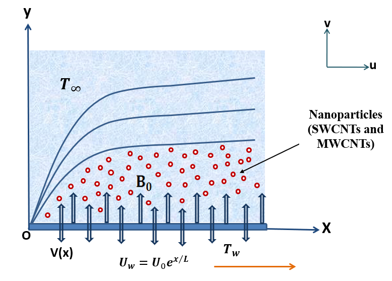
Figure 1: Schematic physical geometry

The thermophysical characteristics [55]-[58] of nanofluids are defined as:

$$\displaystyle\left.\begin{aligned} \begin{aligned} \frac{\mu_{f}}{(1-\phi)^{2.5}}&=\mu_{nf}\quad\\ \frac{\mu_{nf}}{\rho_{nf}}&=\nu{nf},\quad\\ (1-\phi)\rho_{f}+\phi\rho_{CNT}&=\rho_{nf},\quad\\ (1-\phi)(\rho C_{p})_{f}+\phi(\rho C_{p})_{CNT}&=(\rho C_{p})_{nf},\\ {K_{f}}\left(\frac{(K_{CNT}+2K_{f})-2\phi(K_{f}-K_{CNT})}{(K_{CNT}+2K_{f})+\phi(K_{f}-K_{CNT})}\right)&={K_{nf}}.\\ \end{aligned}\end{aligned}\right\}$$ (5)

Here volume concentration of nanomaterial is defined by $\displaystyle\phi$, kinematic viscidity of nanofluid represents $\displaystyle\nu_{nf}$, effective viscosity of base fluid and nanofluid reflected by $\displaystyle\mu_{f}$ and $\displaystyle\mu_{nf}$ respectively. The basic fluid has a density $\displaystyle\rho_{f}$. The explicit warmth of base fluid and CNTs are described by $\displaystyle(\rho C_{p})_{f}$ and $\displaystyle(\rho C_{p})_{CNT}$ correspondingly, while potential to conduct heat of base fluid is designated through $\displaystyle K_{f}$ and thermal conduction of CNTs are $\displaystyle K_{CNT}$.

The thermophysical significance of the nanoaparticles (CNTs) and base fluid (kerosene oil) is displayed in table 1.

Properties	Base Fluid	Nanoparticles
	Kerosene Oil	SWCNT	MWCNT
$\displaystyle\rho$	783	2600	1600
$\displaystyle C_{p}$	2090	425	796
$\displaystyle K$	0.145	6600	3000

Table 1: Data of Thermophysical properties of kerosene oil and CNTs [59]-[60].

2.1 Boundary Conditions

The corresponding boundary conditions for the study are as follows [61]:

$$\displaystyle\begin{aligned} u&=U_{w}+N\nu_{nf}\frac{\partial u}{\partial y},\quad&v&=-V(x),\quad&T&=T_{w}+D\frac{\partial T}{\partial y},\quad&\mbox{at}\ y&=0,\\ u&\rightarrow 0,\quad&T&\rightarrow T_{\infty},\qquad&\mbox{as}\ y&\rightarrow\infty.\end{aligned}$$ (6)

Here $\displaystyle U_{w}=U_{0}e^{\frac{x}{L}}$ is the stretching velocity, where the reference velocity is indicated with $\displaystyle U_{0}$, $\displaystyle N=N_{1}e^{\frac{-x}{2L}}$ is the initial velocity slip factor which changes with $\displaystyle x$, the minimum value of the velocity drop part is $\displaystyle N_{1}$, $\displaystyle T_{w}=T_{\infty}+T_{0}e^{\frac{x}{2L}}$ is the temperature at the sheet, $\displaystyle T_{0}$ mention reference temperature and $\displaystyle D=D_{1}e^{\frac{-x}{2L}}$ is the thermal slip factor which is also diverse along $\displaystyle x$-axis, $\displaystyle D_{1}$ is the basic value of the thermal slip factor. The no slip case will be covered if $\displaystyle N=D=0$. $\displaystyle V(x)=V_{0}e^{\frac{x}{2L}}$ is assumed a special kind of velocity at the wall, where $\displaystyle V_{0}$ is the initial strength of suction. $\displaystyle V(x)>0$ is the velocity of suction and $\displaystyle V(x)<0$ is the velocity of injection or blasting.

2.2 Solution Mechanism

The accompanying coincidence transformations are proposed to alter the aforementioned set of non-linear partial differential equations (2)-(4) into a set of ordinary differential equations (ODE) together with associated boundary conditions (6).

$$\displaystyle\left.\begin{aligned} \begin{aligned} u&=U_{0}e^{\frac{x}{L}}\ f^{\prime}(\eta),\quad&v&=-\sqrt{\frac{\nu_{f}U_{0}}{2L}}e^{\frac{x}{2L}}\left[f(\eta)+\eta f^{\prime}(\eta)\right],\\ \eta&=y\sqrt{\frac{U_{0}}{2\nu_{f}L}}e^{\frac{x}{2L}},\quad&\psi&=\sqrt{2\nu_{f}LU_{0}}f(\eta)\ e^{\frac{x}{2L}},\\ T&=T_{\infty}+T_{0}\ e^{\frac{x}{2L}}\theta(\eta).\\ \end{aligned}\end{aligned}\right\}$$ (7)

Through injecting the stream function $\displaystyle\psi$, the continuity equation (1) is resolved.

$$\begin{split}u=\frac{\partial\psi}{\partial y},\quad v=-\frac{\partial\psi}{\partial x}.\end{split}$$ (8)

The similarity variable is $\displaystyle\eta$, and the stream function is $\displaystyle\psi$.

Using the similarity transformations (7), the set of translated ordinary differential equations seem to be:

$$\displaystyle\left.\begin{aligned} \begin{aligned} \frac{\mu_{nf}/\mu_{f}}{\rho_{nf}/\rho_{f}}f^{\prime\prime\prime}+ff^{\prime\prime}-2f^{\prime 2}-Kf^{\prime}-Frf^{\prime 2}-Mf^{\prime}=0\\ \left[\frac{1}{Pr}\frac{K_{nf}/K_{f}}{(\rho Cp)_{nf}/(\rho C_{p})_{f}}+\frac{4}{3}R\right]\theta^{\prime\prime}-f^{\prime}\theta+f\theta^{\prime}=0\end{aligned}\end{aligned}\right\}$$ (9)

With the aid of a proper similarity transformation, boundary conditions adopt the following form:

$$\displaystyle\begin{aligned} f(0)&=S,\quad&f^{\prime}(0)&=1+A_{1}\lambda f^{\prime\prime},\quad&\theta(0)&=1+\delta\theta^{\prime},\quad&\mbox{at}\ \eta&=0,\\ f^{\prime}(\infty)&\rightarrow 0,\quad&\theta(\infty)&\rightarrow 0,\quad&\mbox{as}\ \eta&\rightarrow\infty.\end{aligned}$$ (10)

Here, $\displaystyle K=\frac{2\nu_{nf}L}{K_{1}U_{w}}$ is the local porosity parameter, $\displaystyle F_{r}=\frac{c_{b}}{2\sqrt{K_{1}}}$ is the Forchheimer number, $\displaystyle M=\frac{2\sigma B^{2}L}{\rho_{f}U_{w}}$ is the magnetic field parameter, $\displaystyle R=\frac{4\sigma^{*}T^{3}_{\infty}}{K_{nf}K^{*}}$ is thermal radiation parameter, $\displaystyle Pr=\frac{\nu_{f}(\rho Cp)_{f}}{K_{f}}$ is Prandtl number, $\displaystyle S=\frac{V_{0}}{\sqrt{\frac{U_{0}\nu_{f}}{2L}}}>0$ is the suction parameter ($\displaystyle<0$ then its blowing parameter), $\displaystyle\lambda=N_{1}\sqrt{\frac{U_{0}\nu}{2L}}$ is the velocity slip parameter and $\displaystyle\delta=D_{1}\sqrt{\frac{U_{0}}{2\nu L}}$ is the thermal slip parameter. Also, $\displaystyle A_{1}=\left(\frac{1}{(1-\phi)^{2.5}\left(1-\phi+\phi\frac{\rho_{s}}{\rho_{f}}\right)}\right).$

The skin friction coefficient $\displaystyle C_{fx}$ and local Nusselt number $\displaystyle Nu_{x}$ are defined as:

$$\begin{split}C_{fx}=\frac{\tau_{w}}{\rho_{f}U_{w}^{2}},\quad Nu_{x}=\frac{xq_{w}}{k_{f}(T_{w}-T_{\infty})},\quad\end{split}$$ (11)

where $\displaystyle\tau_{w}$ represents skin friction or the shear stress and $\displaystyle q_{w}$ is the surface heat flux and is represented as:

$$\begin{split}\tau_{w}=\mu_{nf}\left(\frac{\partial u}{\partial y}\right)_{y=0}&\mbox{and}\quad q_{w}=-k_{nf}\left(\frac{\partial T}{\partial y}\right)_{y=0},\end{split}$$ (12)

By using the transformation (7) into (11) and (12), the skin friction number and local Nusselt number are now detailed as:

$$\displaystyle\begin{aligned} \sqrt{Re}\ C_{fx}&=\frac{1}{(1-\phi)^{2.5}}f^{\prime\prime}(0),\\ Re_{x}^{\frac{-1}{2}}\ Nu_{x}&=-\frac{K_{nf}}{K_{f}}\sqrt{\frac{x}{2L}}\theta^{\prime}(0).\end{aligned}$$ (13)

Here $\displaystyle Re_{x}=\frac{U_{0}e^{\frac{x}{L}}}{\nu_{f}}$ is the local Reynolds number.

3 Computational Methodology

3.1 bvp4c Algorithm

With multiple choices of the inflow regulating parameters, the nonlinear differential equations (9) and boundary conditions (10) are quantitatively evaluated through using bvp4c simulator in MATLAB software. This three-stage Lobatto IIIa technique has been constructed using only a finite difference approach in the bvp4c solver. In order for this solver to work, users must input a set of preliminary hypotheses among the selections of boundary layer thicknesses. The findings are captured whenever the boundary conditions have been monotonically satisfied and there are not any inaccuracies in MATLAB. Before using the bvp4c algorithm, we should first represent the interconnected non-linear differential equations like a combination with first-order ODEs.

We’ll simply add the predictor attributes.

$$\displaystyle\begin{aligned} h(1)=f,\quad h(2)=f^{\prime},\quad h(3)=f^{\prime\prime}\\ h(4)=\theta,\quad h(5)=\theta^{\prime}\\ \end{aligned}$$

Incorporate the above different variables through into set of equations (9) and generate a new network of first order equations as indicated:

$$\displaystyle\begin{aligned} f^{\prime}&=h(2)\\ f^{\prime\prime}&=h(3)\\ f^{\prime\prime\prime}&=\frac{\rho_{nf}/\rho_{f}}{\mu_{nf}/\mu_{f}}\left[2h(2)^{2}-h(1)h(3)+Kh(2)+Frh(2)^{2}+Mh(2)\right]\\ \theta&=h(4)\\ \theta^{\prime}&=h(5)\\ \theta^{\prime\prime}&=\left[\left(Pr\frac{(\rho Cp)_{nf}/(\rho Cp)_{f}}{K_{nf}/K_{f}}+\frac{3}{4}R\right)\left\{h(2)h(4)-h(1)h(5)\right\}\right]\\ \end{aligned}$$

The boundary conditions (10) are transformed into:

$$\displaystyle\begin{aligned} h_{a}(1)&=S,\quad&h_{a}(2)&=1+A_{1}\lambda h(3),\quad h_{a}(4)&=1+\delta h(5),\\ h_{b}(2)&\rightarrow 0,&\quad h_{b}(4)&\rightarrow 0.\end{aligned}$$

In this case, $\displaystyle h_{a}$ identifies the location of $\displaystyle\eta=0$, and $\displaystyle h_{b}$ reflects the region of $\displaystyle\eta\rightarrow\infty$.

3.2 Keller Box Scheme

Keller box approach is employed to calculate the governing equations (9) as well as the boundary conditions (10). The reliability of this approach is of the second series. The steps listed below can be taken to get the solution:

• Reconstruct the partial differential equations toward first order ordinary differential equations.

• Employ centered-difference estimations to build finite difference interpretations of computations.

• To linearize the equations, apply Newton’s linearization approach (if they are non linear).

• To tackle the restricted system, implement the block-tridiagonal-elimination method.

3.2.1 Transformation to First Order System

To express equations in a first order system, we must innovate additional reliant variables $\displaystyle m(\eta)$, $\displaystyle n(\eta)$, and $\displaystyle o(\eta)$, as a consequence:

$$f^{\prime}=m,\quad m^{\prime}=n,\quad\theta^{\prime}=o,$$ (14)

where $\displaystyle prime(\prime)$ reflects the separation with $\displaystyle\eta$. Accordingly, the non-linear ODEs  (9) can be stated as:

$$\frac{\mu_{nf}/\mu_{f}}{\rho_{nf}/\rho_{f}}n^{\prime}+fn-2m^{2}-Km-Frm^{2}-Mn =0,$$ (15)

$$\left[\frac{1}{Pr}\frac{K_{nf}/K_{f}}{(\rho Cp)_{nf}/(\rho C_{p})_{f}}+\frac{4}{3}R\right]o^{\prime}-m\theta+fo =0,$$ (16)

The boundary conditions  (10) in prospective of the newly reliant variables are given by:

$$\displaystyle\left.\begin{aligned} \begin{aligned} f(0)&=S,\quad m(0)=1+\lambda n(0),\quad\theta(0)=1+\delta o(0),\\ m(\eta)&\rightarrow 0,\quad\theta(\eta)\rightarrow 0.\end{aligned}\end{aligned}\right\}$$ (17)

3.2.2 Finite Difference Scheme

We are now contemplating the division $\displaystyle\eta_{j-1}\eta_{j}$ along the centroid $\displaystyle\eta_{j-1/2}$ , which would be described as:

$$\displaystyle\eta_{0}=0,\quad\eta_{j}=\eta_{j-1}+h_{j},\quad\eta_{j}=\eta_{\infty}$$ (18)

In which $\displaystyle h_{j}$ symbolizes the $\displaystyle\Delta\eta$-spacing and $\displaystyle\Delta\eta=1,2,3,........,J$ is a progression number indicating the correspondent spot. Now the finite difference adjustment to equations (14-16) yield the resulting sequence of equations:

$$\displaystyle f_{j}-f_{j-1}-h_{j}(m_{j}+m_{j-1})/2 \displaystyle=0,$$ (19)

$$\displaystyle m_{j}-m_{j-1}-h_{j}(n_{j}+n_{j-1})/2 \displaystyle=0,$$ (20)

$$\displaystyle\theta_{j}-\theta_{j-1}-h_{j}(o_{j}+o_{j-1})/2 \displaystyle=0,$$ (21)

$$\displaystyle\left(\frac{\mu_{nf}/\mu_{f}}{\rho_{nf}\rho_{f}}\right)\left(n_{j}-n_{j-1}\right)+\left[\frac{h_{j}}{4}\right]\left(f_{j}+f_{j-1}\right)\left(n_{j}+n_{j-1}\right)-2\left[\frac{h_{j}}{4}\right]\left(m_{j}+m_{j-1}\right)^{2}-K\left[\frac{h_{j}}{2}\right]$$

$$\displaystyle\left(m_{j}+m_{j-1}\right)-Fr\left[\frac{h_{j}}{2}\right]\left(m_{j}+m_{j-1}\right)^{2}-M\left[\frac{h_{j}}{2}\right]\left(n_{j}+n_{j-1}\right) \displaystyle=0$$ (22)

$$\displaystyle\left[\left(\frac{1}{Pr}\right)\frac{K_{nf}/K_{f}}{(\rho cp)_{nf}/(\rho cp)_{f}}+\frac{4}{3}R\right]\left(o_{j}-o_{j-1}\right)-\frac{h_{j}}{4}\left[\left(m_{j}+m_{j-1}\right)\left(\theta_{j}+\theta_{j-1}\right)\right]$$

$$\displaystyle+\frac{h_{j}}{4}\left[\left(f_{j}+f_{j-1}\right)\left(o_{j}+o_{j-1}\right)\right] \displaystyle=0.$$ (23)

Following equations are prescribed with $\displaystyle j=1,2,3,.....J-1$, and in addition to the boundary conditions for $\displaystyle j=0$ and $\displaystyle j=J$ are respectively:

$$\left.\begin{aligned} \begin{aligned} f_{0}&=S,\quad m_{0}=1+A_{1}\lambda n(0),\quad\theta_{0}=1+\delta o(0),\\ m_{J}&=0,\quad\theta_{J}=0.\end{aligned}\end{aligned}\right\}$$ (24)

3.2.3 Newton’s Linearization Method

We employed Newton’s method to deal with such nonlinear equations  (19 - 23). For this, we’ve included the iterates [$\displaystyle f_{j}^{i},\leavevmode\nobreak\ m_{j}^{i},\leavevmode\nobreak\ n_{j}^{i},\leavevmode\nobreak\ \theta_{j}^{i},\leavevmode\nobreak\ o_{j}^{i}$], where $\displaystyle i=0,1,2,....$. We configured the appropriate for higher iterations:

$$\displaystyle\begin{aligned} f_{j}^{i+1}&=f_{j}^{i}+\delta f_{j}^{i},\quad&m_{j}^{i+1}&=m_{j}^{i}+\delta m_{j}^{i},\quad&n_{j}^{i+1}&=n_{j}^{i}+\delta n_{j}^{i},\\ \theta_{j}^{i+1}&=\theta_{j}^{i}+\delta\theta_{j}^{i},\quad&o_{j}^{i+1}&=o_{j}^{i}+\delta o_{j}^{i}.\end{aligned}$$ (25)

Subsequently they inserted the right-hand side of such formulations in (19-23), and discarding the complex physical components within $\displaystyle\delta$. Generalized expressions like (remove superscript $\displaystyle i$ for clarification):

$$\displaystyle\left.\begin{aligned} \begin{aligned} \delta f_{j}-\delta f_{j-1}-h_{j}(\delta m_{j}+\delta m_{j-1})/2&=(T_{1})_{j},\\ \delta m_{j}-\delta m_{j-1}-h_{j}(\delta n_{j}+\delta n_{j-1})/2&=(T_{2})_{j},\\ \delta\theta_{j}-\delta\theta_{j-1}-h_{j}(\delta o_{j}+\delta o_{j-1})/2&=(T_{3})_{j},\\ (d_{1})_{j}\delta n_{j}+(d_{2})_{j}\delta n_{j-1}+(d_{3})_{j}\delta f_{j}+(d_{4})_{j}\delta f_{j-1}+(d_{5})_{j}\delta m_{j}+(d_{6})_{j}\delta m_{j-1}&=(T_{4})_{j},\\ (e_{1})_{j}\delta o_{j}+(e_{2})_{j}\delta o_{j-1}+(e_{3})_{j}\delta f_{j}+(e_{4})_{j}\delta f_{j-1}+(e_{5})_{j}\delta m_{j}+(e_{6})_{j}\delta m_{j-1}\\ +(e_{7})_{j}\delta\theta_{j}+(e_{8})_{j}\delta\theta_{j-1}&=(T_{5})_{j}.\end{aligned}\end{aligned}\right\}$$ (26)

where

$$\displaystyle(d_{1})_{j} \displaystyle=\frac{\mu_{nf}/\mu_{f}}{\rho_{nf}\rho_{f}}+\frac{h_{j}}{2}f_{j-1/2}, \displaystyle(d_{2})_{j} \displaystyle=(d_{1})_{j}-2\Bigl{[}\frac{\mu_{nf}/\mu_{f}}{\rho_{nf}\rho_{f}}\Bigr{]}$$

$$\displaystyle(d_{3})_{j} \displaystyle=\frac{h_{j}}{2}n_{j-1/2}, \displaystyle(d_{4})_{j} \displaystyle=(d_{3})_{j},$$

$$\displaystyle(d_{5})_{j} \displaystyle={h_{j}}(2+Fr)m_{j-1/2}-(K+M)\frac{h_{j}}{2}, \displaystyle(d_{6})_{j} \displaystyle=(d_{5})_{j},$$

$$\displaystyle(e_{1})_{j} \displaystyle=-\left[\left(\frac{1}{Pr}\right)\frac{K_{nf}/K_{f}}{(\rho cp)_{nf}/(\rho cp)_{f}}+\frac{4}{3}(R)+\frac{h_{j}}{2}(f_{j-1/2})\right],$$

$$\displaystyle(e_{2})_{j} \displaystyle=(e_{1})_{j}-2\Bigl{[}\left(\frac{1}{Pr}\right)\frac{K_{nf}/K_{f}}{(\rho cp)_{nf}/(\rho cp)_{f}}+\frac{4}{3}(R)\Bigr{]},$$

$$\displaystyle(e_{3})_{j} \displaystyle=\frac{h_{j}}{2}\left(o_{j-1/2}\right), \displaystyle(e_{4})_{j} \displaystyle=(e_{3})_{j},$$

$$\displaystyle(e_{5})_{j} \displaystyle=\frac{h_{j}}{2}h_{j}\left(\theta_{j-\frac{1}{2}}\right), \displaystyle(e_{6})_{j} \displaystyle=(e_{5})_{j},$$

$$\displaystyle(e_{7})_{j} \displaystyle=\frac{h_{j}}{2}\left(m_{j-1/2}\right), \displaystyle(e_{8})_{j} \displaystyle=(e_{7})_{j}.$$

$$\displaystyle(R_{1})_{j} \displaystyle=f_{j-1}-f_{j}+h_{j}m_{j-\frac{1}{2}},$$

$$\displaystyle(R_{2})_{j} \displaystyle=m_{j-1}-m_{j}+h_{j}n_{j-\frac{1}{2}},$$

$$\displaystyle(R_{3})_{j} \displaystyle=\theta_{j-1}-\theta_{j}+h_{j}o_{j-\frac{1}{2}},$$

$$\displaystyle(R_{4})_{j} \displaystyle=\frac{\rho_{nf}/\rho_{f}}{\mu_{nf}/\mu_{f}}(o_{j-1}-o_{j})-h_{j}(fm)_{j-1/2}+h_{j}(2+Fr)m_{j-1/2}^{2}+h_{j}(K+M)m_{j-1/2},$$

$$\displaystyle(R_{5})_{j} \displaystyle=-\Bigl{[}(Pr)\frac{(\rho cp)_{nf}/(\rho cp)_{f}}{(K)_{nf}/(K)_{f}}+\frac{3}{4}(R)\Bigr{]}(o_{j}-o_{j-1})-h_{j}(m\theta)_{j-1/2}-h_{j}(fo)_{j-1/2}.$$

For all iterates, we take the following form respectively:

$$\displaystyle\left.\begin{aligned} \begin{aligned} \delta f_{0}&=0,\quad\delta m_{0}=0,\quad\delta n_{0}=0,\quad\delta\theta_{0}=0,\quad\delta o_{0}=0,\\ \delta m_{J}&=0,\quad\delta\theta_{J}=0.\end{aligned}\end{aligned}\right\}$$ (27)

This merely indicates that the input parameters should stay unchanged across the iteration mechanism.

3.2.4 Block Tridiagonal Structure

The structure does have a block-tridiagonal structure, so the generalised linear pair of equations (26) could be resolved using the block-elimination method described by Cebeci and Bradshaw [62]. Block tridiagonal structures, they are often made up of variables or constants, but in this case, an intriguing aspect is that they are made up of block matrices. The equation is transformed into a matrix vector form as follows:

$$\begin{bmatrix}[D_{1}]&[F_{1}]\\ [E_{2}]&[D_{2}]&[F_{2}]\\ &[E_{3}]&[D_{3}]&[F_{3}]\\ &&&&\ddots&\cdots\\ &&&&&[E_{j-1}]&[D_{j-1}]&[F_{j-1}]\\ &&&&&&[E_{j}]&[D_{j}]\end{bmatrix}\begin{bmatrix}[\delta_{1}]\\ [\delta_{2}]\\ [\delta_{3}]\\ \vdots\\ [\delta_{j-1}]\\ [\delta_{J}]\end{bmatrix}=\begin{bmatrix}[T_{1}]\\ [T_{2}]\\ [T_{3}]\\ \vdots\\ [T_{j-1}]\\ [T_{j}]\end{bmatrix}$$

or

$$[D][\delta]=[T]$$ (28)

where the components of the specified heat mechanism are:

$$\begin{bmatrix}\delta_{1}\end{bmatrix}=\begin{bmatrix}[\delta n_{0}]\\ [\delta o_{0}]\\ [\delta f_{1}]\\ [\delta n_{1}]\\ [\delta o_{1}]\end{bmatrix},\leavevmode\nobreak\ \leavevmode\nobreak\ \begin{bmatrix}\delta_{j}\end{bmatrix}=\begin{bmatrix}[\delta m_{j-1}]\\ [\delta\theta_{j-1}]\\ [\delta f_{j}]\\ [\delta n_{j}]\\ [\delta o_{j}]\end{bmatrix},\leavevmode\nobreak\ \leavevmode\nobreak\ 2\leq j\leq J$$

$$\begin{bmatrix}T_{j}\end{bmatrix}=\begin{bmatrix}(T_{1})_{j}\\ (T_{2})_{j}\\ (T_{3})_{j}\\ (T_{4})_{j}\\ (T_{5})_{j}\end{bmatrix},\leavevmode\nobreak\ \leavevmode\nobreak\ 1\leq j\leq J$$

$$\begin{bmatrix}D_{1}\end{bmatrix}=\begin{bmatrix}0&0&1&0&0\\ d&0&0&d&0\\ 0&d&0&0&d\\ (d_{2})_{1}&0&(d_{3})_{1}&(d_{1})_{1}&0\\ 0&(e_{2})_{1}&(e_{3})_{1}&0&(e_{1})_{1}\end{bmatrix}$$

Now

$$\begin{bmatrix}D_{j}\end{bmatrix}=\begin{bmatrix}d&0&1&0&0\\ -1&0&0&d&0\\ 0&-1&0&0&d\\ (d_{6})_{j}&0&(d_{3})_{j}&(d_{1})_{j}&0\\ (e_{6})_{j}&(e_{8})_{j}&(e_{3})_{j}&0&(e_{1})_{j}\end{bmatrix},\leavevmode\nobreak\ \leavevmode\nobreak\ 2\leq j\leq J$$

$$\begin{bmatrix}E_{j}\end{bmatrix}=\begin{bmatrix}0&0&-1&0&0\\ 0&0&0&d&0\\ 0&0&0&0&d\\ 0&0&(d_{4})_{j}&(d_{2})_{j}&0\\ 0&0&(e_{4})_{j}&0&(e_{2})_{j}\end{bmatrix},\leavevmode\nobreak\ \leavevmode\nobreak\ 2\leq j\leq J$$

$$\begin{bmatrix}F_{j}\end{bmatrix}=\begin{bmatrix}d&0&0&0&0\\ 1&0&0&0&0\\ 0&1&0&0&0\\ (d_{5})_{j}&0&0&0&0\\ (e_{5})_{j}&(e_{7})_{j}&0&0&0\end{bmatrix},\leavevmode\nobreak\ \leavevmode\nobreak\ 1\leq j<J$$

Here $\displaystyle d=-\frac{h_{j}}{2}$.

Now we will figure out the dilemma (28) through Lower-Upper factorisation or decomposition, supposing $\displaystyle D$ is any matrix whose determinant is not zero that could be decomposed into:

$$[D]=[L][U]$$ (29)

where

$$\begin{bmatrix}L\end{bmatrix}=\begin{bmatrix}[\alpha_{1}]\\ [\beta_{2}]&[\alpha_{2}]\\ &&\ddots\\ &&\ddots&[\alpha_{J-1}]\\ &&&[\beta_{J}]&[\alpha_{J}]\end{bmatrix},\leavevmode\nobreak\ \leavevmode\nobreak\ \begin{bmatrix}U\end{bmatrix}=\begin{bmatrix}[I_{1}]&[\Gamma_{1}]\\ &[I]&[\Gamma_{2}]\\ &&\ddots&\ddots\\ &&&[I]&[\Gamma_{J-1}]\\ &&&&[I]\end{bmatrix}$$

While [$\displaystyle I$] represents the $\displaystyle 5\times 5$ matrix as well as [$\displaystyle\alpha j$], [$\displaystyle\Gamma j$], and [$\displaystyle\beta j$] are $\displaystyle 5\times 5$ ordered matrices for whom components are predicted through consecutive expression:

$$\displaystyle\left.\begin{aligned} &=[D_{1}]\\ [D_{1}][\Gamma_{1}]&=[F_{1}]\\ [\alpha_{j}]&=[D_{j}]-[\beta_{j}][\Gamma_{j-1}],\leavevmode\nobreak\ \leavevmode\nobreak\ j=2,3,...J\\ [D_{j}][\Gamma_{j}]&=[F_{j}],\leavevmode\nobreak\ \leavevmode\nobreak\ j=2,3,...J\end{aligned}\right\}$$ (30)

By replacing equation (29) in (28), we acquire:

$$[L][U][\delta]=[R]$$ (31)

Now allow us to define,

$$[U][\delta]=[G]$$ (32)

As just a conclusion, equation (31) produces

$$[L][G]=[R],$$ (33)

where

$$\begin{bmatrix}G\end{bmatrix}=\begin{bmatrix}[G_{1}]\\ [G_{2}]\\ \vdots\\ [G_{j-1}]\\ [G_{j}]\end{bmatrix},\leavevmode\nobreak\ \leavevmode\nobreak\ 1\leq j\leq J$$

In this case, [$\displaystyle Gj$] are column matrices of dimension $\displaystyle 5\times 1$, and entries can be acquired by mathematical analysis (33) like:

$$[\alpha_{1}][G_{1}]=[T_{1}],\leavevmode\nobreak\ \leavevmode\nobreak\ \leavevmode\nobreak\ [\alpha_{j}][G_{j}]=[T_{j}]-[\beta_{j}][G_{j-1}],\leavevmode\nobreak\ \leavevmode\nobreak\ 2\leq j\leq J.$$ (34)

The elements of $\displaystyle\Gamma j$, $\displaystyle\alpha j$, and $\displaystyle Gj$ are determined adopting forward sweep, while the phonemes of $\displaystyle\delta$ are accurately assessed from the equation (32) utilizing backward sweep, and thus the constituents include:

$$[\delta_{J}]=[G_{J}],\leavevmode\nobreak\ \leavevmode\nobreak\ \leavevmode\nobreak\ [\delta_{j}]=[G_{j}]-[\Gamma_{j}][\delta_{j+1}],\leavevmode\nobreak\ \leavevmode\nobreak\ 1\leq j\leq J-1.$$ (35)

Such iterative techniques are carried out till the acceptable convergence criterion is accomplished i.e. $\displaystyle|{\delta v_{0}}^{(i)}|<\epsilon$, where $\displaystyle\epsilon$ is the intended level of precision.

4 Results and Discussion

4.1 Code Verification and Parameter Selection

In the present study, the transmission of heat and circulation of CNTs (SWCNT and MWCNT) with lamp fuel oil as just a base fluid under the influence of thermal jump and velocity slip across an exponentially elaborated plate were explored through the proposed investigation. First, the asymmetric partial differential equations (2)-(4) are modified into a group of nonlinear ordinary differential equations (9) through exploiting appropriate similarity transformations. Then, the set of non-linear differential equations is numerically computed by Keller-box scheme and bvp4c algorithm in MATLAB. Table $\displaystyle 2$ demonstrates the comparative analysis for the character of rate of thermal conduction $\displaystyle\theta^{\prime}(0)$ in the non-appearance of magnetic field i.e. $\displaystyle M=0$, nanoparticle concentrations i.e. $\displaystyle\phi=0$, Forchheimer parameter $\displaystyle Fr=0$, porosity parameter $\displaystyle K=0$ and the radiation effect i.e. $\displaystyle R=0$ for $\displaystyle Cu-$ water based nanofluid for the divergent measurements of $\displaystyle Pr$. The acquired consequences are correlated with Magyari and Keller [45], Ishak [63] and EI. Aziz [64]. They have been established in compliance with historically published studies, as demonstrated in table $\displaystyle 2$. Plots depict the effects of important aspects on profiles of velocity and temperature. Also, the effect of skin friction coefficient parameter and Nusselt number are portrayed through table $\displaystyle 3$ and $\displaystyle 4$ correspondingly. By retaining other factors constant, i.e. $\displaystyle\phi=0.2,Fr=0.25,K=1,M=2,S=0.1,\lambda=0.1,\delta=0.1$, the effect of various flow controlling parameters on the velocity and thermal sketches is demonstrated in figures $\displaystyle 2$ and $\displaystyle 3$ correspondingly.

Pr	Magyari and Keller [45]	Ishak [63]	EI Aziz [64]	Present study
1	0.954782	0.9548	0.954785	0.955885
2	—-	—-	—-	1.47122
3	1.869075	1.8691	1.869074	1.868878
5	2.500135	2.5001	2.500132	2.499982
10	3.660379	3.6604	3.660372	3.660255

Table 2: Comparison to the past studies for temperature values, i.e. $\displaystyle-\theta^{\prime}(0)$ throughout the exclusion of nanofluid, where $\displaystyle K=Fr=0$.

4.2 Graphical and Tabular Analysis

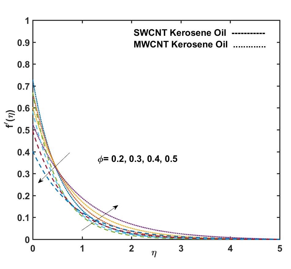
(a) Variation in $\displaystyle f^{\prime}(\eta)$ with $\displaystyle\phi$ against $\displaystyle\eta$

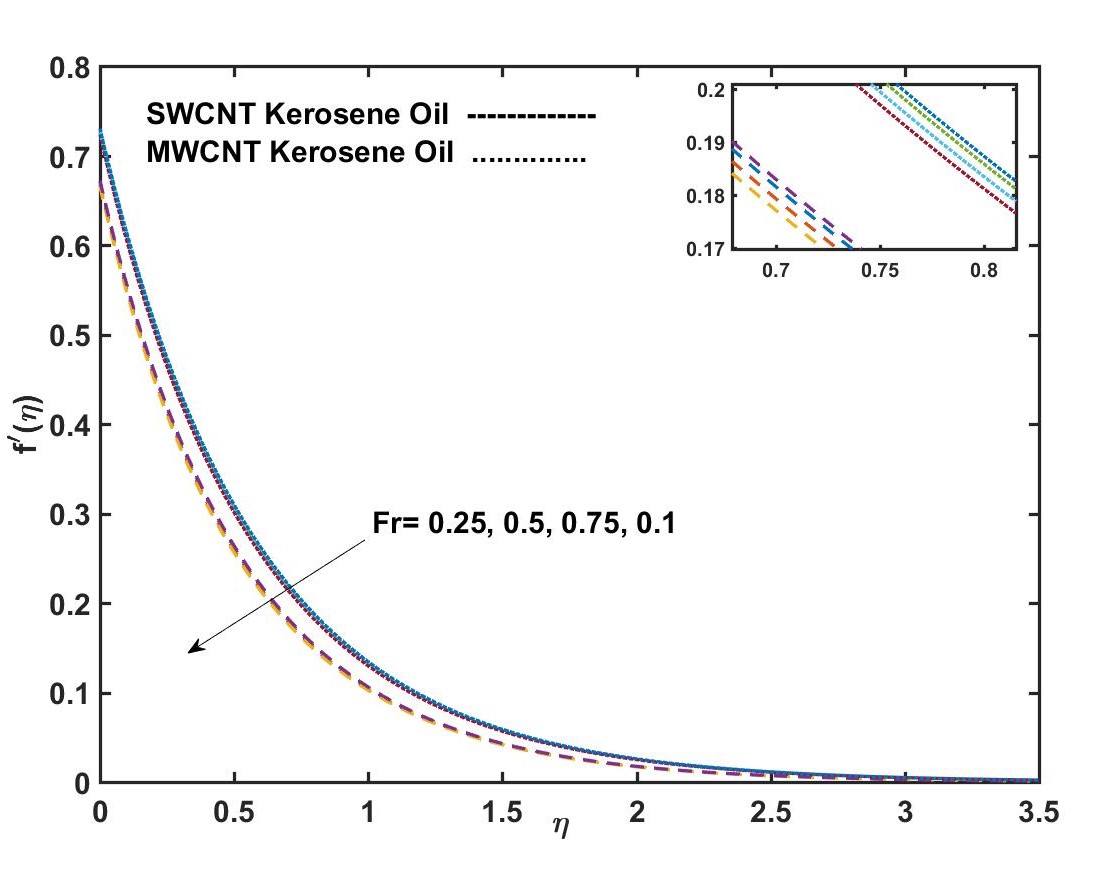
(b) Variation in $\displaystyle f^{\prime}(\eta)$ with $\displaystyle Fr$ against $\displaystyle\eta$

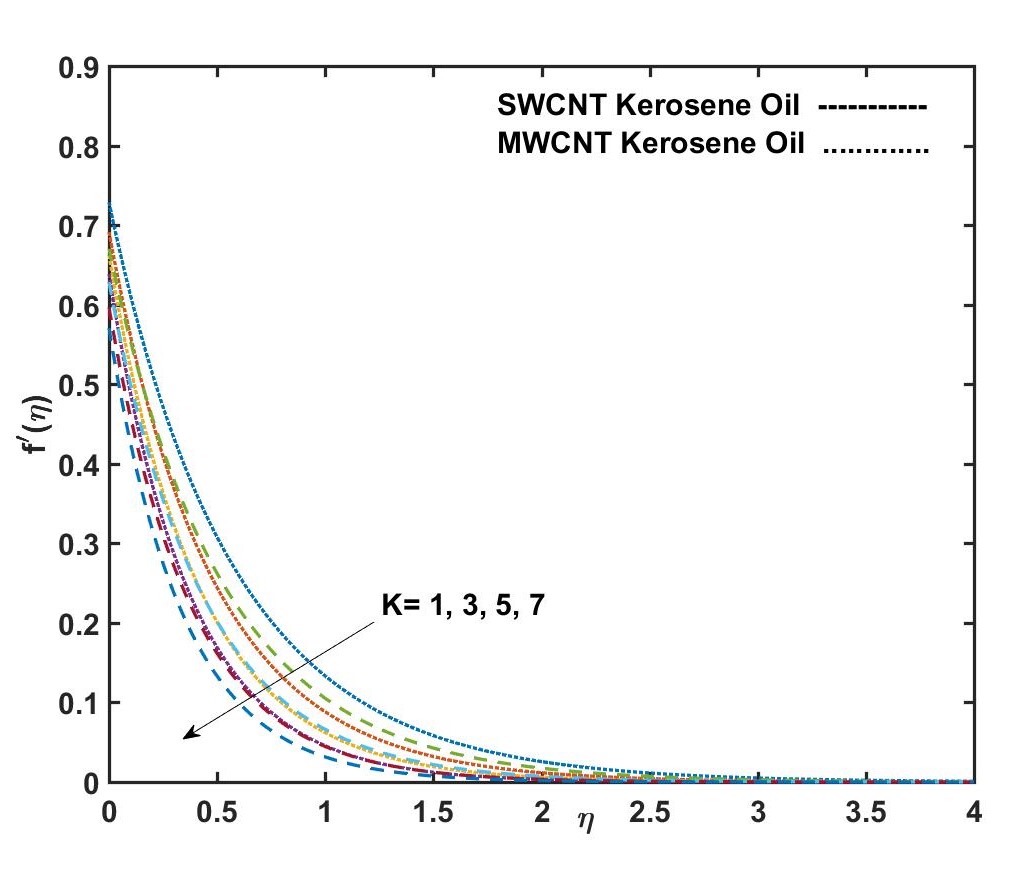
(c) Variation in $\displaystyle f^{\prime}(\eta)$ with $\displaystyle K$ against $\displaystyle\eta$

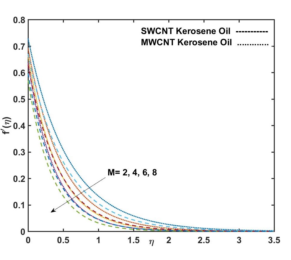
(d) Variation in $\displaystyle f^{\prime}(\eta)$ with $\displaystyle M$ against $\displaystyle\eta$

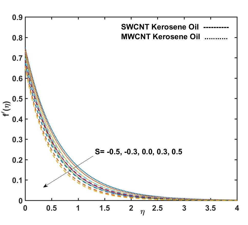
(e) Variation in $\displaystyle f^{\prime}(\eta)$ with $\displaystyle S$ against $\displaystyle\eta$

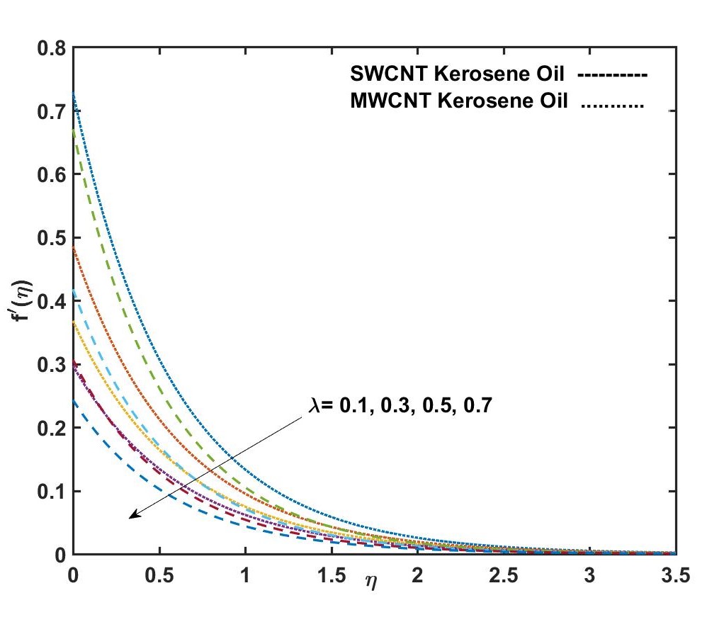
(f) Variation in $\displaystyle f^{\prime}(\eta)$ with $\displaystyle\lambda$ against $\displaystyle\eta$

Figure 2: Alteration in $\displaystyle f^{\prime}(\eta)$ for the distinct values of $\displaystyle\phi$, $\displaystyle Fr$, $\displaystyle K$, $\displaystyle M$, $\displaystyle S$ and $\displaystyle\lambda$

4.2.1 Variation in Velocity Profiles

The velocity profiles of $\displaystyle f^{\prime}(\eta)$ over an exponentially stretched sheet is examined in figure $\displaystyle 2$ by varying flow regulating parameters. Inside the confined zone, the figure $\displaystyle 2(a)$ demonstrates dual phenomena with mounting $\displaystyle\phi$ values. For SWCNTs, the region $\displaystyle 0\leq\eta<0.6$, shows decreasing behaviour, while at $\displaystyle 0.6\leq\eta\leq 1.0$, it shows increasing demeanor with the soaring values of $\displaystyle\phi$. For MWCNTs, in the vicinity $\displaystyle 0\leq\eta<0.5$, it commit collapsing nature, whereas the area $\displaystyle 0.5\leq\eta\leq 1.0$, with increasing values of $\displaystyle\phi$, it displays increasing category. The velocity distribution is found to be the leading function for the enhancement in $\displaystyle\phi$ for SWCNTs and MWCNTs. The accession in the percentage of nanomaterials causes an increase in the convective flow. Also, it has been observed that $\displaystyle f^{\prime}(\eta)$ increases for lamp fuel oil nanoliquid as long as MWCNTs when related to SWCNTs.

Figure $\displaystyle 2(b)$ is outlined to inspect that, by virtue of the velocity profile $\displaystyle f^{\prime}(\eta)$ is distressed by the accumulation in $\displaystyle Fr$. From the sketch, it has been illustrated that the velocity graph reduces for both SWCNTs and MWCNTs with the increasing values of the inertia coefficient $\displaystyle Fr$.

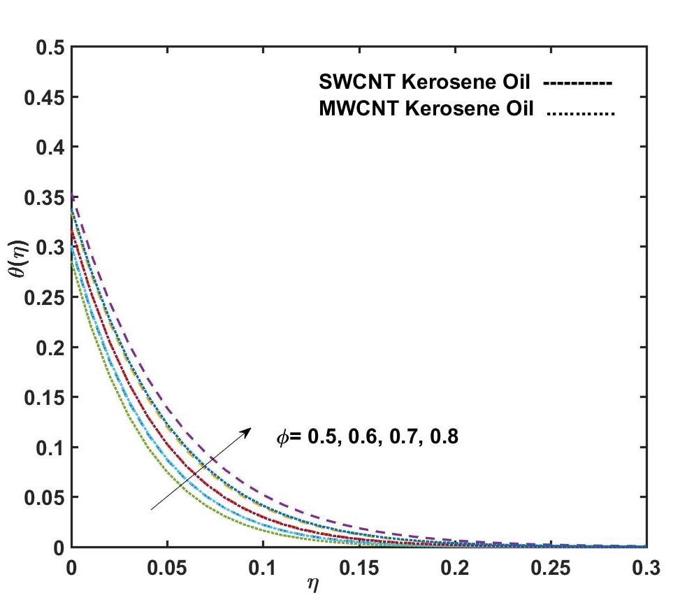
(a) Variation in $\displaystyle\theta(\eta)$ with $\displaystyle\phi$ against $\displaystyle\eta$

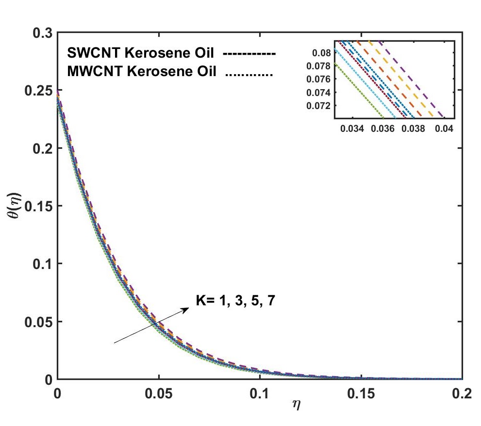
(b) Variation in $\displaystyle\theta(\eta)$ with $\displaystyle K$ against $\displaystyle\eta$

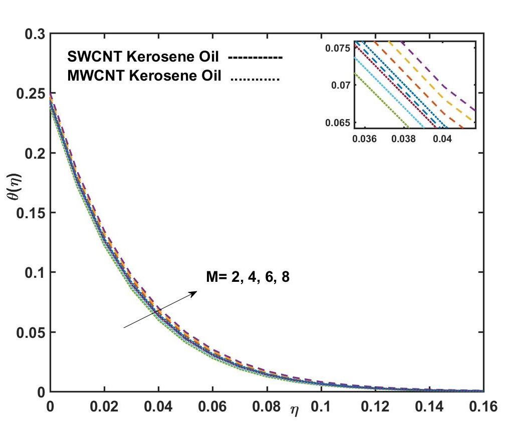
(c) Variation in $\displaystyle\theta(\eta)$ with $\displaystyle M$ against $\displaystyle\eta$

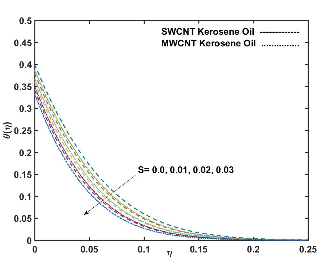
(d) Variation in $\displaystyle\theta(\eta)$ with $\displaystyle S$ against $\displaystyle\eta$

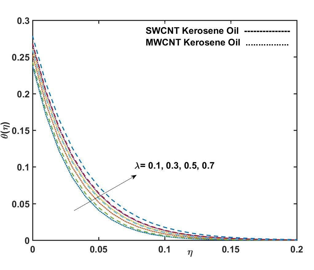
(e) Variation in $\displaystyle\theta(\eta)$ with $\displaystyle\lambda$ against $\displaystyle\eta$

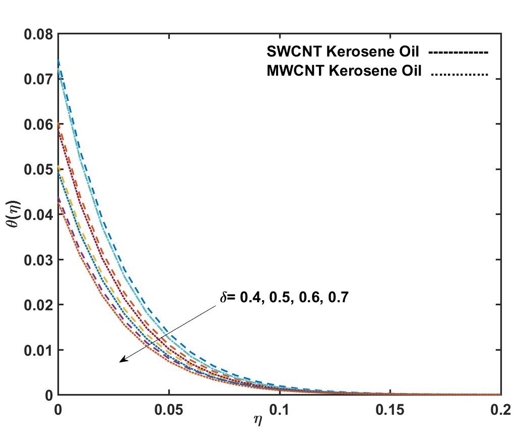
(f) Variation in $\displaystyle\theta(\eta)$ with $\displaystyle\delta$ against $\displaystyle\eta$

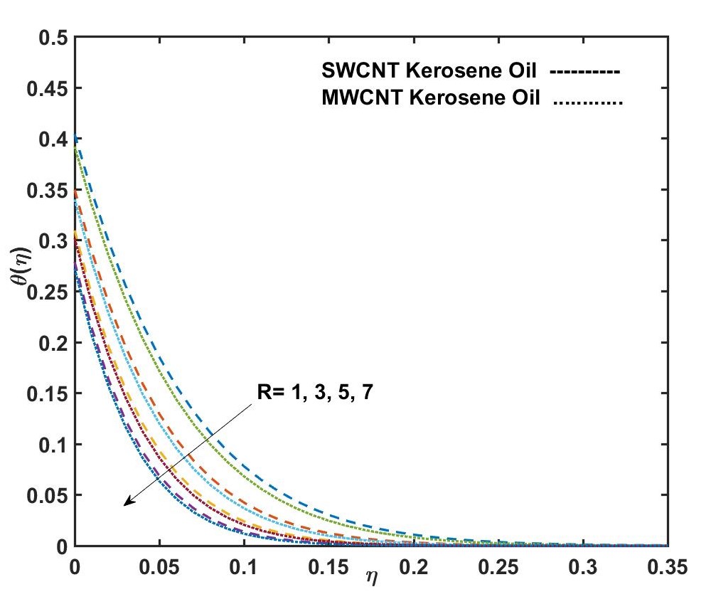
(g) Variation in $\displaystyle\theta(\eta)$ with $\displaystyle R$ against $\displaystyle\eta$

Figure 3: Alteration in $\displaystyle\theta(\eta)$ for the distinct values of $\displaystyle\phi$, $\displaystyle K$, $\displaystyle M$, $\displaystyle S$, $\displaystyle\lambda$, $\displaystyle\delta$ and $\displaystyle R$

Figure $\displaystyle 2(c)$ interprets the change in velocity field $\displaystyle f^{\prime}(\eta)$ with the fluctuating values of the porosity parameter $\displaystyle K$. It has been prove that with the larger values of $\displaystyle K$, the velocity profile $\displaystyle f^{\prime}(\eta)$ decreases simultaneously for both SWCNTs and MWCNTs. For lamp fuel oil based nanofluids, the flow appears to significantly slow down in the axial direction at high values of the porosity parameter $\displaystyle K$. Apparently, the flow intransigence hikes whenever a porous medium is introduced. Furthermore, for lamp fuel oil base liquid, the velocity distribution of SWNTs is wider than that of MWNTs.

Figure $\displaystyle 2(d)$ highlights the implication of the boosting values of magnetic parameter $\displaystyle M$ on the velocity field. It is concluded that for the increment in the attitude of the magnetic field, the velocity profile shows a reduction in their behaviour for SWCNTs and MWCNTs. For higher magnetic estimator predictions, the velocity $\displaystyle f^{\prime}(\eta)$ and associated boundary layer diminish simultaneously. The upsurge in $\displaystyle M$ represents a spike in insusceptible potential (Lorentz force), and hence the velocity of the liquid decelerates. It is also reported that MWCNT kerosene oil seems to have a dominating velocity distribution whenever compared to SWCNT kerosene oil.

Figure $\displaystyle 2(e)$ depicts the dominance of the suction or blowing parameter $\displaystyle S$ on the velocity profile $\displaystyle f^{\prime}(\eta)$. From the figure, it has been detected that the velocity field downturns significantly with the increment in the suction parameter $\displaystyle S$ whereas the blowing parameter shows an increment in the velocity field. Whenever the wall suction $\displaystyle(S>0)$ is addressed, the boundary layer density diminishes and the velocity field reduces. $\displaystyle S=0$ reflects the scenario of a non-porous stretched plate. It is discovered that raising the suction parameter greatly decreases fluid velocity, whereas blowing increases the fluid velocity.

The effect of velocity slip parameter $\displaystyle\lambda$ on velocity profile $\displaystyle f^{\prime}(\eta)$ is delineated in figure $\displaystyle 2(f)$. The velocity graph $\displaystyle 2(f)$ illustrates that as the sheet’s distance $\displaystyle(\eta)$ climbs, the transit rate declines. The velocity disappears at a certain large distance from the sheet (at $\displaystyle\eta=3.5$ in all cases). As a result, horizontal velocity decreases as $\displaystyle\lambda$ increases. When the layer slides, the flow rate all around the plate never approaches the elongating mobility of the material. Because the stretching sheet’s pulling can only be moderately disclosed under the slide condition to the liquid, similar slip velocity increases as $\displaystyle\lambda$ increases. It should be noted that $\displaystyle\lambda$ has a momentous impact on the CNTs. Also, it is recognised that the kersoene-SWCNTs have higher velocity than kerosene MWCNTs.

4.2.2 Variation in Thermal Profiles

Figure $\displaystyle 3$ scrutinize the consequences of diverse outflow predominating parameters on the thermal profile $\displaystyle\theta(\eta)$ over an exponentially stretched sheet. The ramification of expanding values of volume fraction $\displaystyle\phi$ on the thermal profile $\displaystyle\theta(\eta)$ is portrayed in figure $\displaystyle 3(a)$. It is noticed that the temperature profile increases with the increasing character of $\displaystyle\phi$ for both SWCNTs and MWCNTs. This is caused by the addition of carbon nanotubes. The thermal conductivity of the fluid increases vastly because of the very high rate of thermal transmission of CNTs in comparison with other nanomaterials. Moreover, it is also noticed that the temperature profile for SWCNTs is greater as compared to MWCNTs.

Figure $\displaystyle 3(b)$ depicts the change in temperature portrait as the porosity parameter $\displaystyle K$ is varied. For the larger values of $\displaystyle K$, an enhancement is noticed in the temperature profile $\displaystyle\theta(\eta)$ for both SWCNTs and MWCNTs. The temperature profile in figure $\displaystyle 3(c)$ is seen to be significantly increased with the escalating values of magnetic parameter $\displaystyle M$ for both SWCNTs and MWCNTs. The existence of a magnetic field $\displaystyle M$ reduces the density of the momentum boundary layer while increasing the density of the thermal boundary layer.

Figure $\displaystyle 3(d)$ depicts how a change in the suction/blowing parameter $\displaystyle S$ alters the thermal sketch $\displaystyle\theta(\eta)$, resulting a reduction in the nature of both SWCNTs and MWCNTs. From the figure, it is seen that the temperature profile decelerates as the suction variable $\displaystyle S$ is elevated. As a result, the effect of the suction/blowing parameter is to maximise the amount of thermal transmission from the surface to the neighbouring fluid. Bringing vacuum fluids virtually towards the interface region means that solutions exhibit a spacious flow separation, and thus the density of a momentum pressure gradient is reduced.

The behaviour of $\displaystyle\theta(\eta)$ for varying ethics of the velocity lapse parameter $\displaystyle\lambda$ is advertised in figure $\displaystyle 3(e)$. It is found that the thermal sketch shows that with the increment in the character of the velocity blunder framework $\displaystyle\lambda$, the temperature profile also boosted for both SWCNTs and MWCNTs. From the figure, it has been detected that the thermal portrait is greater for SWCNTs as correlated to MWCNTs.

Meanwhile, temperature jump $\displaystyle\delta$ in figure $\displaystyle 3(f)$, shows a reduction with the increment in $\displaystyle\delta$ for both SWCNTs and MWCNTs. The temperature profile initially declines with $\displaystyle\delta$, but over a certain separation $\displaystyle\eta$ from the sheet, this component fades entirely. As the $\displaystyle\delta$ improves, limited warmth is transported towards the liquid from the plate, and therefore the temperature decreases gradually. Figure $\displaystyle 3(g)$ depicts the behaviour of the temperature profile $\displaystyle\theta(\eta)$ with the ascending radiation parameter $\displaystyle R$. It has been established that when $\displaystyle R$ is raised, the surface heat transmission capacity comes to a halt.

$\displaystyle\phi$	$\displaystyle M$	$\displaystyle Fr$	$\displaystyle K$	$\displaystyle S$	$\displaystyle\lambda$	$\displaystyle-\frac{1}{(1-\phi)^{2.5}}f^{\prime\prime}(0)$
						SWCNT	MWCNT
0.02	0.1	0.2	0.1	0.1	0.1	1.2486	1.2408
0.05						1.3070	1.2894
0.07						1.3455	1.3227
0.1	1.0					1.6504	1.6211
	1.5					1.7640	1.7352
	2.0					1.8658	1.8379
	2.5	0.1				1.9493	1.9222
		0.2				1.9581	1.9315
		0.3				1.9668	1.9406
		0.4	0.1			1.9754	1.9497
			0.3			2.0095	1.9843
			0.5			2.0424	2.0179
			0.7	0.1		2.0744	2.0504
				0.2		2.1074	2.0824
				0.4		2.1746	2.1476
				0.5	0.1	2.2088	2.1807
					0.4	1.1861	1.2330
					0.7	0.8184	0.8678
					0.9	0.6793	0.7260

Table 3: Alteration in $\displaystyle-\frac{1}{(1-\phi)^{2.5}}f^{\prime\prime}(0)$ for a variety of input variables with $\displaystyle Pr=21$.

$\displaystyle\phi$	$\displaystyle M$	$\displaystyle Fr$	$\displaystyle K$	$\displaystyle R$	$\displaystyle S$	$\displaystyle\lambda$	$\displaystyle\delta$	$\displaystyle-{\frac{K_{nf}}{K_{f}}}\theta^{\prime}(0)$
								SWCNT	MWCNT
0.02	0.1	0.2	0.1	10	0.1	0.1	0.1	8.5023	8.5062
0.05								9.1959	9.2067
0.07								9.6799	9.6963
0.1	1.0							10.4209	10.4493
	1.5							10.4110	10.4406
	2.0							10.4020	10.4327
	2.5	0.1						10.3946	10.4261
		0.2						10.3938	10.4253
		0.3						10.3930	10.4246
		0.4	0.1					10.3923	10.4239
			0.3					10.3891	10.4212
			0.5					10.3861	10.4184
			0.7	1				8.7329	8.8044
				5				9.6695	9.7172
				7				9.9964	10.0369
				10	0.1			10.3832	10.4158
					0.2			11.3612	11.3788
					0.4			12.1877	12.1964
					0.5	0.1		12.3909	12.3978
						0.4		12.3830	12.3903
						0.7		12.3799	12.3871
						0.9	0.1	12.3787	12.3858
							0.15	8.4542	8.4574
							0.17	7.5027	7.5053
							0.19	6.7438	6.7458

Table 4: Alteration in $\displaystyle-{\frac{K_{nf}}{K_{f}}}\theta^{\prime}(0)$ for a variety of input variables with $\displaystyle Pr=21$.

4.2.3 Variation in Coefficient of Skin Friction and Rate of Heat Transmission

The divergence in skin friction coefficient and Nusselt number estimates with the growing ethics of volume fraction $\displaystyle\phi$, magnetic parameter $\displaystyle M$, Forchheimer parameter $\displaystyle Fr$, porosity parameter $\displaystyle K$, radiation parameter $\displaystyle R$, suction parameter $\displaystyle S$, velocity slip parameter $\displaystyle\lambda$ and temperature jump parameter $\displaystyle\delta$ are displayed in table $\displaystyle 3$ and $\displaystyle 4$. In table $\displaystyle 3$, an enhancement in the SWCNTs and MWCNTs is made up of the surged volume fraction of the nano materials, magnetic number, Forchheimer number, porosity parameter, and suction parameter. However, SWCNT and MWCNT were reduced with the improving values of $\displaystyle\lambda$. However, the coefficient of skin friction and rate of heat transmission climb at the surface as the nanomaterial volume fraction rises. This is because adding CNTs to nanofluids makes them more viscous, which improves heat conductivity. From the table $\displaystyle 4$, it is seen that the Nusselt number inflates in the pair of SWCNTs and MWCNTs with the accession values of $\displaystyle R$ and $\displaystyle S$ whereas it decreases with the increment in $\displaystyle M$, $\displaystyle Fr$, $\displaystyle K$, $\displaystyle\lambda$ and $\displaystyle\delta$.

5 Conclusion

In the current investigation, the 2-dimensional boundary layer ciculation of nanofluid containing carbon nanotubes (CNTs) under the influence of thermal radiation, velocity slip, and temperature fluctuation throughout an exponentially extending layer is addressed. In this work, lamp fuel oil is employed as a conventional fluid for the extraction of CNT-based nanoparticles. There are two standard forms of CNTs that were introduced, named single-walled carbon nanotubes (SWCNTs) and multi-walled carbon nanotubes (MWCNTs) for concentration in the working fluid. Both the bvp4c algorithm and the Keller-box technique in MATLAB software are employed to evaluate the set of nonlinear equations (9) and boundary conditions (10). The consequences of various flow modulating non-dimensional characteristics on velocity, temperature, coefficient of skin friction , and rate of thermal transmission are tested and provided graphically and tabularly. The key themes of the ongoing investigation are listed below:

• When the nanoparticle concentration climbs, MWCNTs generate an inflate in the velocity field relative to SWCNTs and a dual solution occurs in the velocity field.

• The velocity diminishes as the velocity slip grows. Temperature is reduced as the thermal blunder framework is improved.

• The suction criterion $\displaystyle S$ dwindled the fluid velocity and temperature with their growing values. Also, the temperature field is reduced as the radiation parameter $\displaystyle R$ is enhanced.

• An enhancement is engraved in skin friction coefficient with the increasing values of volume fraction of nanoparticles $\displaystyle\phi$, magnetic parameter $\displaystyle M$, inertia coefficient $\displaystyle Fr$, porosity parameter $\displaystyle K$ and suction $\displaystyle S$ for both considered nanoparticles (SWCNTs and MWCNTs), while it reduces for the pair of (SWCNTs and MWCNTs) with the increment in velocity slip.

• The heat transmission rate shows an increment with the improvement in volume fraction of nanoparticles, radiation and suction parameters respectively. However, an opposite trend is examined in magnetic parameters, inertia coefficient, porosity parameter, velocity slip, and temperature jump for SWCNTs and MWCNTs.

Compliance with Ethical Standards

Declarations of Originality

The author declares that no similar work has been done earlier by anyone and takes full responsibility of the originality of the figures and graphs presented in this work.

Funding

Not applicable.

Conflicts of interest

There is no conflict of interest.

Availability of data and material

Not applicable.

References

- [1] Choi, S.U.S. and Eastman, J.A., 1995. Enhancing thermal conductivity of fluids with nanoparticles (No. ANL/MSD/CP-84938; CONF-951135-29). Argonne National Laboratory, IL (United States).
- [2] Kim, Y.J., Shin, T.S., Do Choi, H., Kwon, J.H., Chung, Y.C. and Yoon, H.G., 2005. Electrical conductivity of chemically modified multiwalled carbon nanotube/epoxy composites. Carbon, 43(1), pp.23-30.
- [3] Ma, X., Su, F., Chen, J., Bai, T. and Han, Z., 2009. Enhancement of bubble absorption process using a CNTs-ammonia binary nanofluid. International Communications in Heat and Mass Transfer, 36(7), pp.657-660.
- [4] Ding, Y., Alias, H., Wen, D. and Williams, R.A., 2006. Heat transfer of aqueous suspensions of carbon nanotubes (CNT nanofluids). International Journal of Heat and Mass Transfer, 49(1-2), pp.240-250.
- [5] Choi, J. and Zhang, Y., 1995. Properties and Applications of Single-, Double- and Multi-Walled Carbon Nanotubes. In Aldrich Materials Science, Sigma-Aldrich Co. LLC: Steinheim, Germany.
- [6] Iijima, S., 1991. Helical microtubules of graphitic carbon. Nature, 354(6348), pp.56-58.
- [7] Mare, T., Halelfadl, S., Sow, O., Estelle, P., Duret, S. and Bazantay, F., 2011. Comparison of the thermal performances of two nanofluids at low temperature in a plate heat exchanger. Experimental Thermal and Fluid Science, 35(8), pp.1535-1543.
- [8] Liu, M.S., Lin, M.C.C., Huang, I.T. and Wang, C.C., 2005. Enhancement of thermal conductivity with carbon nanotube for nanofluids. International communications in Heat and Mass Transfer, 32(9), pp.1202-1210.
- [9] De Volder, M.F., Tawfick, S.H., Baughman, R.H. and Hart, A.J., 2013. Carbon nanotubes: present and future commercial applications. Science, 339(6119), pp.535-539.
- [10] Said, Z., Saidur, R., Rahim, N.A. and Alim, M.A., 2014. Analyses of exergy efficiency and pumping power for a conventional flat plate solar collector using SWCNTs based nanofluid. Energy and Buildings, 78, pp.1-9.
- [11] Xue, Q.Z., 2005. Model for thermal conductivity of carbon nanotube-based composites. Physica B: Condensed Matter, 368(1-4), pp.302-307.
- [12] Khan, W.A., Khan, Z.H. and Rahi, M., 2014. Fluid flow and heat transfer of carbon nanotubes along a flat plate with Navier slip boundary. Applied Nanoscience, 4(5), pp.633-641.
- [13] Turkyilmazoglu, M., 2015. Analytical solutions of single and multi-phase models for the condensation of nanofluid film flow and heat transfer. European Journal of Mechanics-B/Fluids, 53, pp.272-277.
- [14] Manevitch, L.I., Smirnov, V.V., Strozzi, M. and Pellicano, F., 2017. Nonlinear optical vibrations of single-walled carbon nanotubes. International Journal of Non-Linear Mechanics, 94, pp.351-361.
- [15] Lee, S., Choi, S.S., Li, S.A. and Eastman, J.A., 1999. Measuring thermal conductivity of fluids containing oxide nanoparticles.
- [16] Aman, S., Khan, I., Ismail, Z., Salleh, M.Z. and Al-Mdallal, Q.M., 2017. Heat transfer enhancement in free convection flow of CNTs Maxwell nanofluids with four different types of molecular liquids. Scientific reports, 7(1), pp.1-13.
- [17] Khorasanizadeh, H., Nikfar, M. and Amani, J., 2013. Entropy generation of Cu–water nanofluid mixed convection in a cavity. European Journal of Mechanics-B/Fluids, 37, pp.143-152.
- [18] Soleimani, H., Baig, M.K., Yahya, N., Khodapanah, L., Sabet, M., Demiral, B.M. and Burda, M., 2018. Impact of carbon nanotubes based nanofluid on oil recovery efficiency using core flooding. Results in Physics, 9, pp.39-48.
- [19] Taherian, H., Alvarado, J.L. and Languri, E.M., 2018. Enhanced thermophysical properties of multiwalled carbon nanotubes based nanofluids. Part 1: Critical review. Renewable and Sustainable Energy Reviews, 82, pp.4326-4336.
- [20] Wang, R., Xie, L., Hameed, S., Wang, C. and Ying, Y., 2018. Mechanisms and applications of carbon nanotubes in terahertz devices: A review. Carbon, 132, pp.42-58..
- [21] Haq, R.U., Khan, Z.H., Khan, W.A. and Shah, I.A., 2017. Viscous dissipation effects in water driven carbon nanotubes along a stream wise and cross flow direction. International Journal of Chemical Reactor Engineering, 15(1).
- [22] Garg, P., Alvarado, J.L., Marsh, C., Carlson, T.A., Kessler, D.A. and Annamalai, K., 2009. An experimental study on the effect of ultrasonication on viscosity and heat transfer performance of multi-wall carbon nanotube-based aqueous nanofluids. International Journal of Heat and Mass Transfer, 52(21-22), pp.5090-5101.
- [23] Imtiaz, M., Hayat, T., Alsaedi, A. and Ahmad, B., 2016. Convective flow of carbon nanotubes between rotating stretchable disks with thermal radiation effects. International Journal of Heat and Mass Transfer, 101, pp.948-957.
- [24] Kumaresan, V., Velraj, R. and Das, S.K., 2012. Convective heat transfer characteristics of secondary refrigerant based CNT nanofluids in a tubular heat exchanger. International Journal of Refrigeration, 35(8), pp.2287-2296.
- [25] Karimipour, A., Bagherzadeh, S.A., Taghipour, A., Abdollahi, A. and Safaei, M.R., 2019. A novel nonlinear regression model of SVR as a substitute for ANN to predict conductivity of MWCNT-/water hybrid nanofluid based on empirical data. Physica A Statistical Mechanics and its Applications, 521, pp.89-97.
- [26] Karimipour, A., D’Orazio, A. and Goodarzi, M., 2018. Develop the lattice Boltzmann method to simulate the slip velocity and temperature domain of buoyancy forces of FMWCNT nanoparticles in water through a micro flow imposed to the specified heat flux. Physica A Statistical Mechanics and Its Applications, 509, pp.729-745.
- [27] Safaei, M.R., Togun, H., Vafai, K., Kazi, S.N. and Badarudin, A., 2014. Investigation of heat transfer enhancement in a forward-facing contracting channel using FMWCNT nanofluids. Numerical Heat Transfer, Part A: Applications, 66(12), pp.1321-1340.
- [28] Jalali, E., Ali Akbari, O., Sarafraz, M.M., Abbas, T. and Safaei, M.R., 2019. Heat transfer of oil/MWCNT nanofluid jet injection inside a rectangular microchannel. Symmetry, 11(6), pp.757.
- [29] Rout, H., Mohapatra, S.S., Shaw, S., Pandey, V.S. and Nayak, M.K., 2022. Entropy Optimized Electrohydromagnetic Rotating Flow of Non Newtonian Fluid with Suspension of SWCNT/MWCNT Nanomaterials: Modified Hamilton Crosser Model. Journal of Nanofluids, 11(1), pp.1-16.
- [30] Bagherzadeh, S.A., D’Orazio, A., Karimipour, A., Goodarzi, M. and Bach, Q.V., 2019. A novel sensitivity analysis model of EANN for F-MWCNTs– nanofluid thermal conductivity: Outputs predicted analytically instead of numerically to more accuracy and less costs. Physica A Statistical Mechanics and Its Applications, 521, pp.406-415.
- [31] Ghasemi, A., Hassani, M., Goodarzi, M., Afrand, M. and Manafi, S., 2019. Appraising influence of -MWCNTs on thermal conductivity of antifreeze using curve fitting and neural network. Physica A Statistical Mechanics and its Applications, 514, pp.36-45.
- [32] Forchheimer, P., 1901. Wasserbewegung durch boden. Z. Ver. Deutsch, Ing., 45, pp.1782-1788.
- [33] Muskat, M., 1946. The flow of homogeneous fluids through porous media: Ann Arbor. Michigan, JW Edwards, 763.
- [34] Seddeek, M.A., 2006. Influence of viscous dissipation and thermophoresis on Darcy–Forchheimer mixed convection in a fluid saturated porous media. Journal of Colloid and Interface Science, 293(1), pp.137-142.
- [35] Sadiq, M.A. and Hayat, T., 2016. Darcy–Forchheimer flow of magneto Maxwell liquid bounded by convectively heated sheet. Results in physics, 6, pp.884-890.
- [36] Hayat, T., Haider, F., Muhammad, T. and Alsaedi, A., 2017. On Darcy-Forchheimer flow of carbon nanotubes due to a rotating disk. International Journal of Heat and Mass Transfer, 112, pp.248-254.
- [37] Iqbal, Z., Azhar, E. and Maraj, E.N., 2017. Transport phenomena of carbon nanotubes and bioconvection nanoparticles on stagnation point flow in presence of induced magnetic field. Physica E: Low-dimensional Systems and Nanostructures, 91, pp.128-135.
- [38] Hayat, T., Haider, F., Muhammad, T. and Alsaedi, A., 2017. Three-dimensional rotating flow of carbon nanotubes with Darcy-Forchheimer porous medium. Plos one, 12(7), pp.0179576.
- [39] Hayat, T., Khan, M.I., Waqas, M., Alsaedi, A. and Farooq, M., 2017. Numerical simulation for melting heat transfer and radiation effects in stagnation point flow of carbon–water nanofluid. Computer methods in applied mechanics and engineering, 315, pp.1011-1024.
- [40] Sadiq, M.A., Waqas, M. and Hayat, T., 2017. Importance of Darcy-Forchheimer relation in chemically reactive radiating flow towards convectively heated surface. Journal of Molecular Liquids, 248, pp.1071-1077.
- [41] Hayat, T., Shah, F., Alsaedi, A. and Hussain, Z., 2017. Outcome of homogeneous and heterogeneous reactions in Darcy-Forchheimer flow with nonlinear thermal radiation and convective condition. Results in physics, 7, pp.2497-2505.
- [42] Hayat, T., Haider, F., Muhammad, T. and Alsaedi, A., 2017. Darcy-Forchheimer flow due to a curved stretching surface with Cattaneo-Christov double diffusion: A numerical study. Results in physics, 7, pp.2663-2670.
- [43] Muhammad, T., Alsaedi, A., Hayat, T. and Shehzad, S.A., 2017. A revised model for Darcy-Forchheimer three-dimensional flow of nanofluid subject to convective boundary condition. Results in physics, 7, pp.2791-2797.
- [44] Mishra, S.R., Sharma, R.P., Tinker, S. and Panda, G.K., 2022. Impact of Slip and the Entropy Generation in a Darcy-Forchhimer Nanofluid Past a Curved Stretching Sheet with Heterogeneous and Homogenous Chemical Reactions. Journal of Nanofluids, 11(1), pp.48-57.
- [45] Magyari, E. and Keller, B., 1999. Heat and mass transfer in the boundary layers on an exponentially stretching continuous surface. Journal of Physics, 32(5), pp.577.
- [46] Sanjayanand, E. and Khan, S.K., 2006. On heat and mass transfer in a viscoelastic boundary layer flow over an exponentially stretching sheet. International Journal of Thermal Sciences, 45(8), pp.819-828.
- [47] Bidin, B. and Nazar, R., 2009. Numerical solution of the boundary layer flow over an exponentially stretching sheet with thermal radiation. European journal of scientific research, 33(4), pp.710-717.
- [48] Nadeem, S., Hayat, T., Malika, M.Y. and Rajputa, S.A., 2010. Thermal radiation effects on the flow by an exponentially stretching surface: a series solution. Zeitschrift für Naturforschung A, 65(6-7), pp.495-503.
- [49] Nadeem, S., Zaheer, S. and Fang, T., 2011. Effects of thermal radiation on the boundary layer flow of a Jeffrey fluid over an exponentially stretching surface. Numerical Algorithms, 57(2), pp.187-205.
- [50] Nadeem, S. and Lee, C., 2012. Boundary layer flow of nanofluid over an exponentially stretching surface. Nanoscale Research Letters, 7(1), pp.1-6.
- [51] Bhattacharyya, K., 2011. Boundary layer flow and heat transfer over an exponentially shrinking sheet. Chinese Physics Letters, 28(7), pp.074701.
- [52] Sharma, R. and Ishak, A., 2014. Second order slip flow of cu-water nanofluid over a stretching sheet with heat transfer. WSEAS Trans. Fluid Mechanics, 9, pp.26-33.
- [53] Gholami, M.R., Akbari, O.A., Marzban, A., Toghraie, D., Shabani, G.A.S. and Zarringhalam, M., 2018. The effect of rib shape on the behavior of laminar flow of oil/MWCNT nanofluid in a rectangular microchannel. Journal of Thermal Analysis and Calorimetry, 134(3), pp.1611-1628.
- [54] Bhattacharyya, K., Layek, G.C. and Gorla, R.S.R., 2012. Slip effect on boundary layer flow on a moving flat plate in a parallel free stream. International Journal of Fluid Mechanics Research, 39(5).
- [55] Hussain, S.T., Khan, Z.H. and Nadeem, S., 2016. Water driven flow of carbon nanotubes in a rotating channel. Journal of Molecular Liquids, 214, pp.136-144.
- [56] Haq, R.U., Rashid, I. and Khan, Z.H., 2017. Effects of aligned magnetic field and CNTs in two different base fluids over a moving slip surface. Journal of Molecular Liquids, 243, pp.682-688.
- [57] Haq, R.U., Kazmi, S.N. and Mekkaoui, T., 2017. Thermal management of water based SWCNTs enclosed in a partially heated trapezoidal cavity via FEM. International Journal of Heat and Mass Transfer, 112, pp.972-982.
- [58] Haq, R.U., Kazmi, S.N. and Mekkaoui, T., 2017. Thermal management of water based SWCNTs enclosed in a partially heated trapezoidal cavity via FEM. International Journal of Heat and Mass Transfer, 112, pp.972-982.
- [59] Hone, J., 2004. Carbon nanotubes thermal properties. Dekker Encyclopedia of Nanoscience and Nanotechnology, 7, pp.603-610.
- [60] Ruoff, R.S. and Lorents, D.C., 1995. Mechanical and thermal properties of carbon nanotubes. Carbon, 33(7), pp.925-930.
- [61] Mukhopadhyay, S., 2013. Slip effects on MHD boundary layer flow over an exponentially stretching sheet with suction/blowing and thermal radiation. Ain Shams Engineering Journal, 4(3), pp.485-491.
- [62] Cebeci, T. and Bradshaw, P., 1998. Physical and computational aspects of convective heat transfer. Springer, New York.
- [63] Ishak, A., 2011. MHD boundary layer flow due to an exponentially stretching sheet with radiation effect. Sains Malaysiana, 40(4), pp.391-395.
- [64] Abd El-Aziz, M., 2009. Viscous dissipation effect on mixed convection flow of a micropolar fluid over an exponentially stretching sheet. Canadian Journal of Physics, 87(4), pp.359-368.