Domain-decomposed Bayesian inversion based on local Karhunen-Loève expansions

Abstract

In many Bayesian inverse problems the goal is to recover a spatially varying random field. Such problems are often computationally challenging especially when the forward model is governed by complex partial differential equations (PDEs). The challenge is particularly severe when the spatial domain is large and the unknown random field needs to be represented by a high-dimensional parameter. In this paper, we present a domain-decomposed method to attack the dimensionality issue and the method decomposes the spatial domain and the parameter domain simultaneously. On each subdomain, a local Karhunen-Loève (KL) expansion is constructed, and a local inversion problem is solved independently in a parallel manner, and more importantly, in a lower-dimensional space. After local posterior samples are generated through conducting Markov chain Monte Carlo (MCMC) simulations on subdomains, a novel projection procedure is developed to effectively reconstruct the global field. In addition, the domain decomposition interface conditions are dealt with an adaptive Gaussian process-based fitting strategy. Numerical examples are provided to demonstrate the performance of the proposed method.

1 Introduction

Many real world inverse problems involve forward models governed by partial differential equations (PDEs), and in these problems often the primary task is to recover spatially varying unknown parameters from noisy and incomplete observations. Such problems are ubiquitous in various scientific areas, including geosciences [1], climate prediction [2], seismic inversion [3] and remote sensing [4]. The Bayesian inference [5, 6, 7, 8, 9, 10, 11, 12, 13, 14] has become an important tool for solving such problems, largely due to its ability to quantify the uncertainty in the solutions obtained.

While the Bayesian methods are conceptually straightforward, their applications to the aforementioned PDE-involved inverse problems can be extremely challenging, where a major difficulty lies in the computational aspect. As is well known, in most practical problems, the posterior distributions are analytically intractable, and are often computed with sampling methods. One of the most popular methods in this context is the Markov chain Monte Carlo (MCMC) simulation [15]. The major limitation associated with MCMC as well as other sampling methods is that they typically require a very large number of evaluations of the forward model, which can be prohibitively costly for our problems, as the PDE-involved forward model is computationally intensive. While considerable efforts have been devoted to reducing the computational cost, e.g., [12, 16, 17, 18, 19], many challenges remain in applying the Bayesian methods for the PDE-involved inverse problems. Among them, the dimensionality issue is one of the most frequently encountered difficulties in these problems.

To conduct Bayesian inference, one first needs to parametrize the spatially varying unknown parameter (in Bayesian inference it is typically modelled as a random field) as a finite-dimensional parameter. Existing methods for doing so include the Karhunen-Loève (KL) expansion [20, 21], wavelet-based parameterization [22], and parameterization techniques based on deep generative models (DGM) [23]. In this paper, we focus on the KL expansion since it is optimal in the mean squared error sense with respect to the number of random variables in the representation. In many practical problems, especially those with large spatial domains, often a large number of KL modes are needed to represent the unknown field, leading to a very high-dimensional inference problem. The primary goal of this work is to address this issue and reduce the dimensionality of the inverse problems using a domain decomposition (DD) approach. In particular, we perform domain decomposition over the spatial domain and the parameter space simultaneously. The resulting method enables parallelization and thus facilitates efficient sampling in a much lower dimensional parameter space.

In general, domain decomposition for uncertainty quantification and inverse problems gains a lot of interests, and related methods are actively developed. In [24], local polynomial chaos expansions based on domain decomposition are proposed for solving PDEs with high dimensional random inputs. In [25], we provide a domain-decomposed uncertainty quantification approach based on importance sampling. Efficient methods to compute dominant KL terms through domain decomposition and the corresponding accelerated Monte Carlo sampling procedures are presented in [26, 27]. Domain decomposition methods for solving nonlinear transient inverse heat conduction problems are studied in [28]. In [29, 30, 31], domain decomposition methods with physics-informed neural networks are addressed for forward and inverse problems.

In this work, we focus on domain decomposition for Bayesian inversion, and the main contributions of this work are as follows. The first is effective local representation for priors. It is known that when the unknown fields have complex structures, the corresponding global priors need to have short correlation lengths to give effective inference results, which requires high-dimensional global parameterization. In the method proposed in this work, relative correlation lengths are increased along with decomposing a global spatial domain into small subdomains, such that low-dimensional parameters can approximate complex priors well. The second is efficient forward model evaluation procedures. As discussed above, main computational costs of sampling based inference methods are caused by repetitively evaluating expensive forward models, especially for models governed by PDEs. High-fidelity numerical schemes can give accurate predictions for the outputs of these PDEs, e.g., the finite element methods with a posteriori error bounds [32, 33], but they can be expensive, as they require a large number of degrees of freedom when the underlying model is complex. As the global spatial domain is decomposed in our setting, the finite element degrees of freedom on local subdomains are significantly smaller than those for the global domain, and therefore evaluating each local model is clearly cheaper than evaluating the global model. The third is a new reconstruction approach for the global unknown field. Once local inversions are conducted, directly stitching local fields to approximate global unknown fields can give misleading information on domain decomposition interfaces. For this purpose, our new approach conducts projection of the local inference results over the space spanned by the global KL modes, which gives an effective approximation for the global true field. Lastly, to give proper interface conditions, Gaussian process (GP) models for interface treatments are built with an active learning procedure.

The rest of this paper is organized as follows. Section 2 sets the problem, where the standard MCMC procedure and the KL expansion are reviewed. In Section 3, we discuss the KL expansion on local subdomains, and give our reconstruction procedure for the global input fields. In Section 4, our Gaussian process interface treatments are discussed, and our overall domain-decomposed Markov chain Monte Carlo (DD-MCMC) algorithm is presented. Numerical results are discussed in Section 5. Section 6 concludes the paper.

2 Problem setup

In this section, we briefly review the general description of Bayesian formulation for inference and detailed settings for KL expansion parameterization for PDEs with random inputs.

2.1 Bayesian inverse problem

Letting $\xi$ denote a $N_{\xi}$-dimensional parameter of interest and $\bm{d}_{\text{obs}}\in\mathbb{R}^{n}(n\ll N_{\xi})$ denote $n$-dimensional observed data, we want to estimate $\xi$ from $\bm{d}_{\text{obs}}$. We assume that there exists a forward model $F$ that maps the unknown parameter $\xi$ to the data $\bm{d}_{\text{obs}}$:

$$\bm{d}_{\text{obs}}=F(\xi)+\epsilon\,,$$ (1)

where $\epsilon\in\mathbb{R}^{n}$ denotes the random observation noise and its probability density function is denoted by $\pi_{\epsilon}(\epsilon)$. Then, the likelihood function which characterizes the relationship between observations and the forward model can be defined as

$$\bm{L}(\bm{d}_{\text{obs}}|\xi)=\pi_{\epsilon}(\bm{d}_{\text{obs}}-F(\xi))\,.$$ (2)

In this paper, the noise $\epsilon$ is assumed to be Gaussian with zero mean and a diagonal covariance matrix $\sigma_{\text{obs}}^{2}\bm{I}_{n}$, where $\sigma_{\text{obs}}>0$ is the standard deviation and $\bm{I}_{n}$ is the identity matrix with size $n\times n$. The likelihood function is then proportional to the data-misfit functional $\eta(\xi;\bm{d}_{\text{obs}})\mathrel{\mathop{\mathchar 58\relax}}=\frac{1}{2\sigma^{2}}\|\bm{d}_{\text{obs}}-F(\xi)\|_{2}^{2}$ where $\|\cdot\|_{2}$ denotes the Euclidean norm, i.e.,

$$\bm{L}(\bm{d}_{\text{obs}}|\xi)\propto\exp(-\eta(\xi;\bm{d}_{\text{obs}})).$$

Given a prior distribution $\pi_{0}(\xi)$ of $\xi$ which reflects the knowledge of the parameter before any measurements, based on the Bayes’ rule, the posterior distribution of $\xi$ can be written as

$$\pi(\xi|\bm{d}_{\text{obs}})=\frac{\overbrace{\bm{L}(\bm{d}_{\text{obs}}|\xi)}^{\text{likelihood}}\overbrace{\pi_{0}(\xi)}^{\text{prior}}}{\underbrace{\pi(\bm{d}_{\text{obs}})}_{\text{evidence}}}\propto\bm{L}(\bm{d}_{\text{obs}}|\xi)\pi_{0}(\xi)\,,$$ (3)

where the evidence $\pi(\bm{d}_{\text{obs}})$ in (3) is usually viewed as a normalization constant for a well-defined probability distribution. The posterior distribution is usually analytically intractable, and therefore sampling methods including Markov chain Monte Carlo methods (MCMC) [15] are widely used. A Markov chain is a sequence of samples where the next state only depends on the previous state, which is known as the Markov property, and the move from the current state towards the next state is defined through some transition operator. The MCMC method constructs a Markov chain, of which the equilibrium distribution (also known as the stationary distribution) is set to the target distribution. In the context of Bayesian inversion, the target distribution is the posterior distribution. To ensure the convergence towards the target distribution, the detailed balance condition has to be satisfied. To generate samples of the posterior distribution, we consider the standard Metropolis-Hastings (MH) [34, 35] algorithm, which proceeds as follows. Starting from a randomly chosen initial state, for the $s$-th state $\xi^{s}$, a candidate state $\xi^{\star}$ is drawn from some proposal distribution $Q(\cdot|\xi^{s})$, and then the candidate state is accepted with the probability of an acceptance rate denoted by $\alpha(\xi^{\star},\xi^{s})$. The proposal distribution and the acceptance probability define the transition operator, i.e., $h(\xi^{\star},\xi^{s})=Q(\xi^{\star}|\xi^{s})\alpha(\xi^{\star},\xi^{s}).$ The detailed balance condition is given through the transition operator,

$$\pi(\xi^{s}|\bm{d}_{\text{obs}})h(\xi^{s},\xi^{\star})=\pi(\xi^{\star}|\bm{d}_{\text{obs}})h(\xi^{\star},\xi^{s})\,.$$

To guarantee that the detailed balance condition is satisfied, the acceptance probability can be defined as

$$\alpha(\xi^{\star},\xi^{s})=\min\left\{1,\frac{Q(\xi^{s}|\xi^{\star})\bm{L}(\bm{d}_{\text{obs}}|\xi^{\star})\pi_{0}(\xi^{\star})}{Q(\xi^{\star}|\xi^{s})\bm{L}(\bm{d}_{\text{obs}}|\xi^{s})\pi_{0}(\xi^{s})}\right\}\,.$$

Details of the MH approach is summarized in Algorithm 1, where $N$ is a given number of posterior samples to generate.

Algorithm 1 The standard MH algorithm

1:Forward model $F(\xi)$, observation data $\bm{d}_{\text{obs}}$.

2:Generate an initial state $\xi^{1}$.

3:for $s=1,\ldots,N-1$ do

4:     Draw $\xi^{\star}$ from a proposal distribution $Q(\cdot|\xi^{s})$.

5:     Compute the acceptance ratio

$$\alpha=\min\left\{1,\frac{Q(\xi^{s}|\xi^{\star})\bm{L}(\bm{d}_{\text{obs}}|\xi^{\star})\pi_{0}(\xi^{\star})}{Q(\xi^{\star}|\xi^{s})\bm{L}(\bm{d}_{\text{obs}}|\xi^{s})\pi_{0}(\xi^{s})}\right\}$$

where $\pi_{0}$ is a given prior distribution and the likelihood $\bm{L}$ defined in (2) requires the forward model (1).

6:     Draw $\rho$ from a uniform distribution $\rho\sim\mathcal{U}[0,1]$.

7:     if $\rho<\alpha$ then

8:         Accept the proposal state, i.e., let $\xi^{s+1}=\xi^{\star}$.

9:     else

10:         Reject the proposal state, i.e., let $\xi^{s+1}=\xi^{s}$.

11:     end if

12:end for

13:Posterior samples $\{\xi^{s}\}_{s=1}^{N}$.

2.2 PDEs with random inputs and parameterization

This section presents the detailed settings of the forward model considered in the paper. Let $\mathcal{P}=(\Omega,\Sigma_{\Omega},\mu_{\Omega})$ be a probability space, where $\Omega$ is the set of events, $\Sigma_{\Omega}$ is a sigma-algebra over $\Omega$ and $\mu_{\Omega}$ is a probability measure. We denote the expectation operator for a function $\mathcal{F}(\cdot)$ as

$$\mathbb{E}[\mathcal{F}]=\int_{\Omega}\mathcal{F}(\omega)\operatorname{d\!}\mu_{\Omega}(\omega)\,,$$

and denote $L_{2}(\Omega)$ the space of second-order random variables, i.e., $L_{2}(\Omega)\mathrel{\mathop{\mathchar 58\relax}}=\{\mathcal{F}|\mathbb{E}[\mathcal{F}^{2}]<+\infty\}$. Moreover, $\mathcal{D}\subset\mathbb{R}^{N_{D}}$ ($N_{D}=1,2,3$) denotes a physical domain which is bounded, connected and with a polygonal boundary $\partial\mathcal{D}$, and $x\in\mathcal{D}$ denotes a spatial variable. The space of square integrable functions is defined as $L_{2}(\mathcal{D})\mathrel{\mathop{\mathchar 58\relax}}=\{\mathcal{F}|\int_{\mathcal{D}}\mathcal{F}^{2}<+\infty\}$, and the corresponding inner product is defined as $\langle\mathcal{F}(x),\mathcal{G}(x)\rangle_{\mathcal{D}}\mathrel{\mathop{\mathchar 58\relax}}=\int_{\mathcal{D}}\mathcal{F}(x)\mathcal{G}(x)\operatorname{d\!}x$ for any $\mathcal{F}$ and $\mathcal{G}$ belonging to $L_{2}(\mathcal{D})$. For any $\mathcal{F}\in L_{2}(\mathcal{D})$, the norm induced by the inner product is defined by

$$\|\mathcal{F}\|_{\mathcal{D}}^{2}=\langle\mathcal{F},\mathcal{F}\rangle_{\mathcal{D}}=\int_{\mathcal{D}}\mathcal{F}(x)^{2}\operatorname{d\!}x.$$

The physics of problems considered are governed by a PDE over the spatial domain $\mathcal{D}$ and boundary conditions on the boundary $\partial\mathcal{D}$, which are stated as: find $v(x,\omega)$ mapping $\mathcal{D}\times\Omega$ to $\mathbb{R}$, such that

$$\mathcal{L}(x,v;\kappa(x,\omega))=f(x)\,,\quad x\in\mathcal{D}\,,$$ (4a)

$$\mathcal{B}(x,v;\kappa(x,\omega))=h(x)\,,\quad x\in\partial\mathcal{D}\,,$$ (4b)

where $\mathcal{L}$ is a differential operator and $\mathcal{B}$ is a boundary condition operator, both of which are dependent on a random field $\kappa(x,\omega)$. Here $f$ is the source term and $h$ specifies the boundary condition.

Generally, the random field $\kappa(x,\omega)$ is infinite-dimensional and needs to be parameterized. As the truncated Karhunen-Loève (KL) expansion is an optimal representation of random processes in the mean squared error sense, we focus on this expansion. Letting $a_{0}(x)$ be the mean function of $\kappa(x,\omega)$, the covariance function $C(x,y)\mathrel{\mathop{\mathchar 58\relax}}\mathcal{D}\times\mathcal{D}\to\mathbb{R}$ is defined as

$$C(x,y)=\mathbb{E}[(\kappa(x,\omega)-a_{0}(x))(\kappa(y,\omega)-a_{0}(y))]\,,\quad x,y\in\mathcal{D}\,.$$

We can express the covariance function as $C(x,y)=\sigma(x)\sigma(y)\rho(x,y)$, where $\sigma\mathrel{\mathop{\mathchar 58\relax}}\mathcal{D}\to\mathbb{R}$ is the standard deviation function of the random field and $\rho\mathrel{\mathop{\mathchar 58\relax}}\mathcal{D}\times\mathcal{D}\to[-1,1]$ is its autocorrelation coefficient function. Let $\{\lambda_{r},\psi_{r}(x)\}_{r=1}^{\infty}$ be the eigenvalues and the associated orthonormal eigenfunctions of the covariance function, that is, they satisfy

$$\int_{\mathcal{D}}C(x,y)\psi_{r}(x)\operatorname{d\!}x=\lambda_{r}\psi(y)\,,\quad r=1,2,\ldots,\quad x,y\in\mathcal{D}\,,$$ (5)

and

$$\int_{\mathcal{D}}\psi_{r}(x)\psi_{t}(x)\operatorname{d\!}x=\delta_{rt}\,,$$ (6)

where $\delta_{rt}$ denotes the Kronecker delta, and here we assume that the eigenvalues are ordered in decreasing magnitude. By Mercer’s Theorem, the covariance function has the following spectral decomposition,

$$C(x,y)=\sum_{r=1}^{\infty}\lambda_{r}\psi_{r}(x)\psi_{r}(y)\,.$$

According to the decomposition, it can be seen that $\sum_{r=1}^{\infty}\lambda_{r}=\int_{\mathcal{D}}C(x,x)\operatorname{d\!}x\,.$ Based on the eigen-decomposition of the covariance function, the KL expansion provides a representation in terms of infinite number of random variables,

$$\kappa(x,\omega)=a_{0}(x)+\sum_{r=1}^{\infty}\sqrt{\lambda_{r}}\psi_{r}(x)\xi_{r}(\omega)\,,\quad x\in\mathcal{D}\,,$$ (7)

where $\{\xi_{r}(\omega)\}_{r=1}^{\infty}$ are uncorrelated random variables which control the randomness of the filed. For a given random field $\kappa(x,\omega)$, the corresponding random variables can be given via the orthonormality of eigenfunctions,

$$\xi_{r}(\omega)=\frac{1}{\sqrt{\lambda_{r}}}\int_{\mathcal{D}}[\kappa(x,\omega))-a_{0}(x)]\psi_{r}(x)\operatorname{d\!}x\,,\quad r=1,2,\ldots\,,$$

and satisfy $\mathbb{E}[\xi_{r}]=0$ and $\mathbb{E}[\xi_{r}\xi_{t}]=\delta_{rt}.$ For practical implementations, (7) can be truncated with a finite number of terms such that the leading-order terms are maintained,

$$\kappa(x,\omega)\approx a(x,\xi(\omega))=a_{0}(x)+\sum_{r=1}^{d}\sqrt{\lambda_{r}}\psi_{r}(x)\xi_{r}(\omega)\,,\quad x\in\mathcal{D}\,,$$ (8)

where $\xi(\omega)\mathrel{\mathop{\mathchar 58\relax}}=[\xi_{1}(\omega),\ldots,\xi_{d}(\omega)]^{T}$. In this paper, we refer to $a(x,\xi(\omega))-a_{0}(x)$ as the centralized random field of $a(x,\xi(\omega))$. The truncation level $d$ depends on the decay rate of eigenvalues which is related to the correlation length of the random field. Usually, we select $d$ such that at least $\delta_{\text{KL}}$ (a given threshold) of the total variance is captured, i.e.,

$$\left(\sum_{r=1}^{d}\lambda_{r}\right)/(|\mathcal{D}|\sigma^{2})>\delta_{\text{KL}},$$ (9)

where $|\mathcal{D}|$ denotes the area of the domain $\mathcal{D}$. The prior distribution of $\xi$ is denoted by $\pi_{0}(\xi)$, of which the support is denoted by $I_{\xi}\subset\mathbb{R}^{d}$. For a continuous covariance function, the truncated KL expansion converges in the mean square sense uniformly [36] on $\mathcal{D}$, i.e.,

$$\lim_{d\to\infty}\sup_{x\in\mathcal{D}}\mathbb{E}\left(\kappa(x,\omega)-a_{0}(x)-\sum_{r=1}^{d}\sqrt{\lambda_{r}}\psi_{r}(x)\xi_{r}(\omega)\right)^{2}=0\,.$$

After the above parameterization procedure over the random field, the original governing equation (4) is then transformed into the following finite-dimensional parameterized PDE system: find $u(x,\xi)$ mapping $\mathcal{D}\times I_{\xi}$ to $\mathbb{R}$ such that

$$\mathcal{L}(x,u;a(x,\xi))=f(x)\,,\quad x\in\mathcal{D}\,,$$ (10a)

$$\mathcal{B}(x,u;a(x,\xi))=h(x)\,,\quad x\in\partial\mathcal{D}\,.$$ (10b)

Through specifying an observation operator $\mathfrak{c}$, e.g., taking solution values at several grid points, we write the overall forward model as $F(a(x,\xi))\mathrel{\mathop{\mathchar 58\relax}}=\mathfrak{c}(u(x,\xi))$.

As discussed in detail in [24], for a given random field with correlation length $L_{a}$, the decay rate of the eigenvalues (see (5)) depends on the relative correlation length, i.e., $L_{a,\mathcal{D}}\mathrel{\mathop{\mathchar 58\relax}}=L_{a}/L_{\mathcal{D}}$, where $L_{\mathcal{D}}$ is the diameter of the physical domain $\mathcal{D}$. It is shown that long correlation lengths lead to fast decay of eigenvalues, and vice versa. So, when the correlation length of the global field $\kappa(x,\omega)$ is small, its parameterization over the global domain $\mathcal{D}$ can be high-dimensional (i.e., $d$ in (8) is large). To result in a low-dimensional parameterization, we next decompose the physical domain into small subdomains, and the relative correlation length then becomes larger.

3 Domain-decomposed Parameterization

In this section, we first discuss settings for domain decomposed local problems with KL expansion parameterization posed on subdomains. After that, based on realizations of local KL expansions, a new procedure to reconstruct global permeability fields is presented. These reconstructed global fields are called the assembled fields, and they are shown to be the projections of local fields to the space spanned by global eigenfunctions in KL expansion.

3.1 Local KL expansion parameterization

Our physical domain $\mathcal{D}$ can be represented by a finite number, $M$, of subdomains, i.e., $\overline{\mathcal{D}}=\cup_{i=1}^{M}\overline{\mathcal{D}^{(i)}}$, where $\overline{A}$ denotes the closure of the subset $A$. We consider the case where the intersection of two subdomains can only be a connected interface with a positive $(N_{D}-1)$-dimensional measure or an empty set. For a subdomain $\mathcal{D}^{(i)}$, the set of its boundaries is denoted by $\partial\mathcal{D}^{(i)}$, and the set of its neighboring subdomain indices is denoted by $\mathfrak{N}^{(i)}\mathrel{\mathop{\mathchar 58\relax}}=\{j|j\in\{1,\ldots,M\},j\neq i\text{ and }\partial\mathcal{D}^{(i)}\cap\partial\mathcal{D}^{(j)}\neq\emptyset\}$. The boundary set $\partial\mathcal{D}^{(i)}$ can be split into two parts: external boundaries $\partial\mathcal{D}^{(i)}\cap\partial\mathcal{D}$, and interfaces $\tau^{(i,j)}\mathrel{\mathop{\mathchar 58\relax}}=\partial\mathcal{D}^{(i)}\cap\partial\mathcal{D}^{(j)}$ for $j\in\mathfrak{N}^{(i)}$. Grouping all interface indices associated with all subdomains $\{\mathcal{D}^{(i)}\}_{i=1}^{M}$, we define $\mathfrak{N}\mathrel{\mathop{\mathchar 58\relax}}=\{(i,j)|i\in\{1,2,\ldots,M\}\text{ and }j\in\mathfrak{N}^{(i)}\}.$

We introduce decomposed local operators $\{\mathcal{L}^{(i)}\mathrel{\mathop{\mathchar 58\relax}}=\mathcal{L}|_{\mathcal{D}^{(i)}}\}_{i=1}^{M}$, $\{\mathcal{B}^{(i)}\mathrel{\mathop{\mathchar 58\relax}}=\mathcal{B}|_{\mathcal{D}^{(i)}}\}_{i=1}^{M}$ and local functions $\{f^{(i)}\mathrel{\mathop{\mathchar 58\relax}}=f|_{\mathcal{D}^{(i)}}\}_{i=1}^{M}$, $\{h^{(i)}\mathrel{\mathop{\mathchar 58\relax}}=h|_{\mathcal{D}^{(i)}}\}_{i=1}^{M}$, which are global operators and functions restricted to each subdomain $\mathcal{D}^{(i)}$. The restriction of the field $\kappa(x,\omega)$ to each subdomain is denoted by $\kappa^{(i)}(x,\omega)\mathrel{\mathop{\mathchar 58\relax}}=\kappa(x,\omega)|_{\mathcal{D}^{(i)}}$. For each $i=1,\ldots,M$ and $j\in\mathfrak{N}^{(i)}$, $h^{(i,j)}$ denotes an interface function defined on the interface $\tau^{(i,j)}$, and in this work it is defined as $h^{(i,j)}(x,\omega)\mathrel{\mathop{\mathchar 58\relax}}=v(x,\omega)|_{\tau^{(i,j)}}$, where $v(x,\omega)$ is the solution of the global problem (4). We emphasize that the interface function $h^{(i,j)}$, being the restriction of the global solution on the interface, is dependent on the random input $\omega$. Each local problem is then defined as: for $i=1,\ldots,M$, find $v^{(i)}(x,\omega)\mathrel{\mathop{\mathchar 58\relax}}\mathcal{D}^{(i)}\times\Omega\to\mathbb{R}$ such that

$$\mathcal{L}^{(i)}(x,v^{(i)};\kappa^{(i)}(x,\omega))=f^{(i)}(x)\,,\quad x\in\mathcal{D}^{(i)}\,,$$ (11a)

$$\mathcal{B}^{(i)}(x,v^{(i)};\kappa^{(i)}(x,\omega))=h^{(i)}(x)\,,\quad x\in\partial\mathcal{D}^{(i)}\cap\partial\mathcal{D}\,,$$ (11b)

$$\mathcal{B}^{(i,j)}(x,v^{(i)};\kappa^{(i)}(x,\omega))=h^{(i,j)}(x,\omega)\,,\quad x\in\tau^{(i,j)}\,,\quad j\in\mathfrak{N}^{(i)}\,.$$ (11c)

Eq. (11c) defines the boundary conditions on interfaces and $\mathcal{B}^{(i,j)}$ is an appropriate boundary operator posed on the interface $\tau^{(i,j)}$. With our definition for interface functions, the local problems are consistent with the global problem, i.e.,

$$v(x,\omega)=\begin{cases}v^{(1)}(x,\omega)\,,\quad x\in\overline{\mathcal{D}}^{(1)}\,,\\ \quad\vdots\\ v^{(M)}(x,\omega)\,,\quad x\in\overline{\mathcal{D}}^{(M)}\,.\end{cases}$$

Cf. [25, 37, 24] for detailed discussions for interface functions and boundary conditions for the interfaces.

For each local random field $\kappa^{(i)}(x,\omega)$ for $i=1,\ldots,M$, its mean function is denoted by $a_{0}^{(i)}(x)=a_{0}(x)|_{\mathcal{D}^{(i)}}$, where $a_{0}(x)$ is the mean function of the global field (see (7)). The eigenvalues and the associated orthonormal eigenfunctions of the covariance function posed on each subdomain $\mathcal{D}^{(i)}$ are denoted by $\{\lambda_{r}^{(i)},\psi_{r}^{(i)}\}_{r=1}^{\infty}$ with $\lambda_{1}^{(i)}\geq\lambda_{2}^{(i)}\geq\ldots$, such that

$$\int_{\mathcal{D}^{(i)}}C(x,y)\psi_{r}^{(i)}(x)\operatorname{d\!}x=\lambda_{r}^{(i)}\psi_{r}^{(i)}(y)\,,\quad x,y\in\mathcal{D}^{(i)}\,,$$ (12)

and $\int_{\mathcal{D}^{(i)}}\psi_{r}^{(i)}(x)\psi_{t}^{(j)}(x)\operatorname{d\!}x=\delta_{rt}$. The KL expansion of $\kappa^{(i)}(x,\omega)$ can then be written as

$$\kappa^{(i)}(x,\omega)=a_{0}^{(i)}(x)+\sum_{r=1}^{\infty}\sqrt{\lambda_{r}^{(i)}}\psi_{r}^{(i)}(x)\xi_{r}^{(i)}(\omega)\,,$$ (13)

where $\{\xi^{(i)}_{r}(\omega)\}^{\infty}_{r=1}$ are uncorrelated random variables. Each local random field can be approximated by the truncated KL expansion,

$$\kappa^{(i)}(x,\omega)\approx a^{(i)}(x,\xi^{(i)}(\omega))=a_{0}^{(i)}(x)+\sum_{r=1}^{d^{(i)}}\sqrt{\lambda_{r}^{(i)}}\psi_{r}^{(i)}(x)\xi_{r}^{(i)}(\omega)\,,\quad x\in\mathcal{D}^{(i)}\,,$$ (14)

where $d^{(i)}$ is the number of KL modes retained and $\xi^{(i)}(\omega)\mathrel{\mathop{\mathchar 58\relax}}=[\xi^{(i)}_{1}(\omega),\ldots,\xi^{(i)}_{d^{(i)}}(\omega)]^{T}$ whose element is defined as

$$\xi^{(i)}_{r}(\omega)\mathrel{\mathop{\mathchar 58\relax}}=\frac{1}{\sqrt{\lambda_{r}^{(i)}}}\int_{\mathcal{D}^{(i)}}(a^{(i)}(x,\xi^{(i)}(\omega))-a_{0}^{(i)}(x))\psi_{r}^{(i)}\operatorname{d\!}x.$$ (15)

The error of the truncation depends on the amount of total variance captured, $\delta_{i}\mathrel{\mathop{\mathchar 58\relax}}=\sum_{r=1}^{d^{(i)}}\lambda_{r}^{(i)}/(|\mathcal{D}^{(i)}|\sigma^{2})$, and $d^{(i)}$ needs to be large enough such that $\delta_{i}$ is larger than some given threshold $\delta_{\text{KL}}$.

For $i=1,\ldots,M$, the prior distribution of $\xi^{(i)}$ is denoted by $\pi_{0}(\xi^{(i)})$ with support $I_{\xi^{(i)}}\subset\mathbb{R}^{d^{(i)}}$. For each $i=1,\ldots,M$ and $j\in\mathfrak{N}^{(i)}$, $g^{(i,j)}(x,\xi)$ denotes the interface function $g^{(i,j)}(x,\xi)\mathrel{\mathop{\mathchar 58\relax}}=u(x,\xi)|_{\tau^{(i,j)}}$, where $u(x,\xi)$ is the solution of the parameterized global problem (10). The original local problem (11) is rewritten as: find $u^{(i)}(x,\xi^{(i)})$ mapping $\mathcal{D}^{(i)}\times I_{\xi^{(i)}}$ to $\mathbb{R}$ such that

$$\mathcal{L}^{(i)}(x,u^{(i)};a^{(i)}(x,\xi^{(i)}))=f^{(i)}(x)\,,\quad x\in\mathcal{D}^{(i)}\,,$$ (16a)

$$\mathcal{B}^{(i)}(x,u^{(i)};a^{(i)}(x,\xi^{(i)}))=h^{(i)}(x)\,,\quad x\in\partial\mathcal{D}^{(i)}\cap\partial\mathcal{D}\,,$$ (16b)

$$\mathcal{B}^{(i,j)}(x,u^{(i)};a^{(i)}(x,\xi^{(i)}))=g^{(i,j)}(x,\xi)\,,\quad x\in\tau^{(i,j)}\textrm{ and }j\in\mathfrak{N}^{(i)}\,.$$ (16c)

Defining the observation operator posed on each local subdomain as $\mathfrak{c}^{(i)}\mathrel{\mathop{\mathchar 58\relax}}=\mathfrak{c}|_{\mathcal{D}^{(i)}}$, we denote the local forward model as $F^{(i)}(a^{(i)}(x,\xi^{(i)}))\mathrel{\mathop{\mathchar 58\relax}}=\mathfrak{c}^{(i)}(u^{(i)}(x,\xi^{(i)}))$ and the local observation $\bm{d}_{\text{obs}}^{(i)}\in\mathbb{R}^{n^{(i)}}$ is defined as $\bm{d}_{\text{obs}}^{(i)}=F^{(i)}(a^{(i)}(x,\xi^{(i)}))+\epsilon^{(i)}$, where the local observation noise $\epsilon^{(i)}\sim\mathcal{N}(0,\sigma_{\text{obs}}^{2}\bm{I}_{n^{(i)}})$. Details of our method to efficiently solve the inverse problem posed on each subdomain are discussed in section 4, where samples of the posterior distribution of each local input $\xi^{(i)}$ are generated. The following part of this section is to discuss the procedure of reconstructing the global field $\kappa(x,\omega)$ with given realizations of local inputs $\xi^{(i)}$ for $i=1,\ldots,M$.

3.2 Reconstructed fields

Letting $(\mathcal{D}^{(i)})^{c}\mathrel{\mathop{\mathchar 58\relax}}=\mathcal{D}\setminus\mathcal{D}^{(i)}$ for $i=1,\ldots,M$, extensions of local mean functions and local eigenfunctions to the global domain $\mathcal{D}$ are defined as

$$\widetilde{a}_{0}^{(i)}(x)\mathrel{\mathop{\mathchar 58\relax}}=\begin{cases}a^{(i)}(x)\,,\quad x\in\mathcal{D}^{(i)}\,,\\ 0\,,\quad x\in(\mathcal{D}^{(i)})^{c}\,,\end{cases}$$ (17)

$$\widetilde{\psi}_{r}^{(i)}(x)\mathrel{\mathop{\mathchar 58\relax}}=\begin{cases}\psi_{r}^{(i)}(x)\,,\quad x\in\mathcal{D}^{(i)}\,,\\ 0\,,\quad x\in(\mathcal{D}^{(i)})^{c}\,.\end{cases}$$ (18)

For given realizations of the local inputs, two kinds of reconstructed global fields are introduced in this section, which are called the stitched field and the assembled field respectively in the following.

Definition 1 (The stitched field)

When a realization is given for each local input $\xi^{(i)}$ where $i=1,\ldots,M$, the stitched field $\breve{a}(x,\xi)$ where $\xi^{T}\mathrel{\mathop{\mathchar 58\relax}}=[(\xi^{(1)})^{T},\ldots,(\xi^{(M)})^{T}]$ and $x\in\mathcal{D}$, is defined through directly collecting the corresponding local fields, i.e.,

$$\breve{a}(x,\xi)\mathrel{\mathop{\mathchar 58\relax}}=\sum_{i=1}^{M}\widetilde{a}^{(i)}(x,\xi^{(i)}),$$

where $\widetilde{a}^{(i)}$ is defined as

$$\widetilde{a}^{(i)}(x,\xi^{(i)}) \mathrel{\mathop{\mathchar 58\relax}}=\widetilde{a}_{0}^{(i)}(x)+\sum_{r=1}^{d^{(i)}}\sqrt{\lambda_{r}^{(i)}}\widetilde{\psi}_{r}^{(i)}(x)\xi_{r}^{(i)}.$$ (19)

In (19), $\xi^{(i)}=[\xi^{(i)}_{1},\ldots,\xi^{(i)}_{d^{(i)}}]^{T}$, $\widetilde{a}_{0}^{(i)}(x)$ and $\widetilde{\psi}_{r}^{(i)}(x)$ are defined in (17)–(18), and $\lambda_{r}^{(i)}$ is defined in (12).

As the stitched field is a direct collection of local fields, it can lead to discontinuities on interfaces, and the corresponding inference results can be misleading. To result in an efficient representation of the global field, we define the following assembled field.

Definition 2 (The assembled field)

When a realization is given for each local input $\xi^{(i)}$ where $i=1,\ldots,M$, the assembled field $\widehat{a}(x,\widehat{\xi})$ where $x\in\mathcal{D}$ is defined as

$$\widehat{a}(x,\widehat{\xi})\mathrel{\mathop{\mathchar 58\relax}}=a_{0}(x)+\sum_{t=1}^{d}\sqrt{\lambda_{t}}\psi_{t}(x)\widehat{\xi}_{t}\,,$$ (20)

where $\widehat{\xi}\mathrel{\mathop{\mathchar 58\relax}}=[\widehat{\xi}_{1},\ldots,\widehat{\xi}_{d}]^{T}$, the mean function $a_{0}(x)$ and the eigenpairs $\{\lambda_{t},\psi_{t}(x)\}_{t=1}^{d}$ follow the same settings in (7), and $\{\widehat{\xi}_{t}\}_{t=1}^{d}$ are defined as

$$\widehat{\xi}_{t}=\frac{1}{\sqrt{\lambda_{t}}}\sum_{i=1}^{M}\sum_{r=1}^{d^{(i)}}\sqrt{\lambda_{r}^{(i)}}\xi_{r}^{(i)}\int_{\mathcal{D}^{(i)}}\widetilde{\psi}_{r}^{(i)}(x)\psi_{t}(x)\operatorname{d\!}x\,,\quad t=1,\ldots,d\,.$$ (21)

It can be seen that, the assembled field is represented by the global eigenfunctions, which avoids extra discontinuities on interfaces introduced by the stitched field. In addition, the following theorem shows that the assembled field is the projection of the stitched field over the space spanned by the global eigenfunctions. Therefore, if the truth field is in the space spanned by the global eigenfunctions, the assembled field can typically give a better approximation to the truth field than the stitched field.

Theorem 1

Let $\mathbb{V}_{1}$ denote the space spanned by global eigenfunctions $\{\psi_{r}(x)\}^{d}_{r=1}$ of (5). The centralized assembled field $\widehat{a}(x,\widehat{\xi})-a_{0}(x)$ is the projection of the centralized stitched field $\breve{a}(x,\xi)-a_{0}(x)$ over $\mathbb{V}_{1}$.

Proof 1

For $i=1,\ldots,M$, letting $L_{2}(\mathcal{D}^{(i)})$ denote the space of square integrable functions over $\mathcal{D}^{(i)}$, the inner product of any $\mathcal{F}$ and $\mathcal{G}$ belonging to $L_{2}(\mathcal{D}^{(i)})$ is denoted by $\langle\mathcal{F},\mathcal{G}\rangle_{\mathcal{D}^{(i)}}\mathrel{\mathop{\mathchar 58\relax}}=\int_{\mathcal{D}^{(i)}}\mathcal{F}(x)\mathcal{G}(x)\operatorname{d\!}x$. Denoting $\mathbb{V}_{2}\mathrel{\mathop{\mathchar 58\relax}}={\rm span}\{\widetilde{\psi}_{r}^{(i)}(x),\textrm{ for }i=1,\ldots,M,r=1,\ldots,d^{(i)}\}$, it can be seen that $\widehat{a}(x,\widehat{\xi})-a_{0}(x)\in\mathbb{V}_{1}$ and $\breve{a}(x,\xi)-a_{0}(x)\in\mathbb{V}_{2}$. From (20)–(21), the centralized assembled field can be written as

$$\widehat{a}(x,\widehat{\xi})-a_{0}(x)=\sum_{t=1}^{d}\sqrt{\lambda_{t}}\psi_{t}(x)\widehat{\xi}_{t}=\sum_{t=1}^{d}\sqrt{\lambda_{t}}\psi_{t}(x)\frac{1}{\sqrt{\lambda_{t}}}\sum_{i=1}^{M}\sum_{r=1}^{d^{(i)}}\sqrt{\lambda_{r}^{(i)}}\xi_{r}^{(i)}(\omega)\int_{\mathcal{D}^{(i)}}\widetilde{\psi}_{r}^{(i)}(x)\psi_{t}(x)\operatorname{d\!}x$$

$$\quad=\sum_{t=1}^{d}\sum_{i=1}^{M}\sum_{r=1}^{d^{(i)}}\sqrt{\lambda_{r}^{(i)}}\xi_{r}^{(i)}\langle\widetilde{\psi}_{r}^{(i)},\psi_{t}\rangle_{\mathcal{D}^{(i)}}\psi_{t}(x)=\sum_{t=1}^{d}\left\langle\sum_{i=1}^{M}[\widetilde{a}^{(i)}(x,\xi^{(i)})-\widetilde{a}_{0}^{(i)}(x)],\psi_{t}(x)\right\rangle_{\mathcal{D}}\psi_{t}(x)$$

$$\quad=\sum_{t=1}^{d}\left\langle\breve{a}(x,\xi)-a_{0}(x),\psi_{t}(x)\right\rangle_{\mathcal{D}}\psi_{t}(x).$$ (22)

It can be seen from (22) that the centralized assembled field is the projection of the stitched field $[\breve{a}(x,\xi)-a_{0}(x)]$ over $\mathbb{V}_{1}$.

For a global field $a(x,\xi)$, i.e., (8) with a given realization of $\xi$, we have that $a(x,\xi)-\widehat{a}(x,\widehat{\xi})\in\mathbb{V}_{1}$. For each basis function $\psi_{r}(x)$ of $\mathbb{V}_{1}$ (for $r=1,\ldots,d$), Theorem 1 gives that,

$$\langle\widehat{a}(x,\widehat{\xi})-\breve{a}(x,\xi),\psi_{r}\rangle_{\mathcal{D}}=\left\langle\sum_{t=1}^{d}\langle\breve{a}(x,\xi)-a_{0}(x),\psi_{t}\rangle_{\mathcal{D}}\psi_{t}+a_{0}(x)-\breve{a}(x,\xi),\psi_{r}\right\rangle_{\mathcal{D}}$$

$$=\sum_{t=1}^{d}\langle\breve{a}(x,\xi)-a_{0}(x),\psi_{t}\rangle_{\mathcal{D}}\langle\psi_{t},\psi_{r}\rangle_{\mathcal{D}}-\langle\breve{a}(x,\xi)-a_{0}(x),\psi_{r}\rangle_{\mathcal{D}}=0\,.$$

So, $\langle\widehat{a}(x,\widehat{\xi})-\breve{a}(x,\xi),a(x,\xi)-\widehat{a}(x,\widehat{\xi})\rangle_{\mathcal{D}}=0$. Then,

$$\|a(x,\xi)-\breve{a}(x,\xi)\|_{\mathcal{D}}^{2}=\|a(x,\xi)-\widehat{a}(x,\widehat{\xi})+\widehat{a}(x,\widehat{\xi})-\breve{a}(x,\xi)\|_{\mathcal{D}}^{2}$$

$$\quad=\|a(x,\xi)-\widehat{a}(x,\widehat{\xi})\|_{\mathcal{D}}^{2}+2\langle\widehat{a}(x,\widehat{\xi})-\breve{a}(x,\xi),a(x,\xi)-\widehat{a}(x,\widehat{\xi})\rangle_{\mathcal{D}}+\|\widehat{a}(x,\widehat{\xi})-\breve{a}(x,\xi)\|_{\mathcal{D}}^{2}$$

$$\quad=\|a(x,\xi)-\widehat{a}(x,\widehat{\xi})\|_{\mathcal{D}}^{2}+\|\widehat{a}(x,\widehat{\xi})-\breve{a}(x,\xi)\|_{\mathcal{D}}^{2}.$$

Thus, $\|a(x,\xi)-\widehat{a}(x,\widehat{\xi})\|_{\mathcal{D}}\leq\|a(x,\xi)-\breve{a}(x,\xi)\|_{\mathcal{D}}$, which implies that, if the given field $a(x,\xi)$ is the truth field of our inverse problem, the approximation $\widehat{a}(x,\widehat{\xi})$ is typically more accurate than $\breve{a}(x,\xi)$.

4 Domain-Decomposed Markov chain Monte Carlo (DD-MCMC)

Our goal is to efficiently generate samples of the posterior distribution of the unknown field $a(x,\xi)$ in the global problem (10) through solving local problems (16). In this section, we first propose a new adaptive Gaussian process (GP) interface model for each local problem, and then present our overall DD-MCMC algorithm.

4.1 Adaptive Guassian process for interface treatments

To include measurement locations, the set consisting of observed data is denoted by $S\mathrel{\mathop{\mathchar 58\relax}}=\{(x^{s},d_{\text{obs}}^{s})\}_{s=1}^{n}$, where $x^{s}$ is the location of the $s$-th sensor and $d_{\text{obs}}^{s}\in\mathbb{R}$ is the observation collected at $x^{s}$. The set consisting of all sensor locations is defined by $\bm{x}_{\text{obs}}\mathrel{\mathop{\mathchar 58\relax}}=\{x|(x,d_{\text{obs}})\in S\}$, and the observed data are collected as $\bm{d}_{\text{obs}}=[d_{\text{obs}}^{1},\ldots,d_{\text{obs}}^{n}]^{T}$. For each subdomain $\mathcal{D}^{(i)}$ (for $i=1,\ldots,M$), the set consisting of local observed data is defined as $S^{(i)}\mathrel{\mathop{\mathchar 58\relax}}=\{(x,d_{\text{obs}})|(x,d_{\text{obs}})\in S\textrm{ and }x\in\mathcal{D}^{(i)}\cup\partial\mathcal{D}^{(i)}\}$, of which the size is denoted by $n^{(i)}$, and $\bm{d}_{\text{obs}}^{(i)}\in\mathbb{R}^{n^{(i)}}$ collects observed data contained in $S^{(i)}$.

In each local problem (16), proper interface functions need to be specified. Based on observed data, we build a Gaussian process (GP) model to approximate each interface function, which is a widely used tool to approximate unknown function [38]. From Section 3.1, the interface functions to be specified can be considered as the restrictions of the solution of the global problem associated with the unknown truth sample of the global parameter $\xi$. That is, for each interface $\tau^{(i,j)}$ where $(i,j)\in\mathfrak{N}$, an unknown target function is defined as $\widetilde{g}^{(i,j)}(x)\mathrel{\mathop{\mathchar 58\relax}}=g^{(i,j)}(x,\xi)$. For each target function, its training set is denoted by $\Lambda^{(i,j)}=\{(x^{s},d_{\text{obs}}^{s})\}_{s=1}^{n^{(i,j)}}$ whose size is denoted by $n^{(i,j)}\mathrel{\mathop{\mathchar 58\relax}}=|\Lambda^{(i,j)}|$. The set consisting of the sensor locations in $\Lambda^{(i,j)}$ is denoted by $\bm{x}_{\text{obs}}^{(i,j)}\mathrel{\mathop{\mathchar 58\relax}}=\{x|(x,d_{\text{obs}})\in\Lambda^{(i,j)}\}$, and $\bm{d}_{\text{obs}}^{(i,j)}\in\mathbb{R}^{n^{(i,j)}}$ collects all observations in $\Lambda^{(i,j)}$. Details for constructing the training set and the GP model for the target functions are presented as follows.

A Gaussian process is a collection of random variables, and any finite combinations of these random variables are joint Gaussian distributions. In our setting, for each of $x$, $\widetilde{g}^{(i,j)}(x)$ is considered to be a random variable in a Gaussian process. Each of the prior GP models is denoted by $\widetilde{g}^{(i,j)}(x)\sim\mathcal{GP}(\mu(x),k(x,x^{\prime}))$ where $\mu(\cdot)$ is the mean function and $k(\cdot,\cdot)$ is the kernel of the Gaussian process. The Gaussian process is specified by its mean function and kernel function [38]. In this work, we use the Gaussian kernel, i.e., $k(x,y)=\sigma_{f}^{2}\exp(-\|x-y\|_{2}^{2}/(2l_{f}^{2})$, where the signal variance $\sigma_{f}$ and the length-scale $l_{f}$ are both hyper-parameters of the kernel function. Denoting $\gamma=[\sigma_{f},l_{f}]^{T}$, for a given training data set $\Lambda^{(i,j)}$, the hyper-parameters can be determined through minimizing the negative log marginal likelihood $\mathcal{M}(\gamma)$:

$$\mathcal{M}(\gamma)\mathrel{\mathop{\mathchar 58\relax}} =-\log p(\Lambda^{(i,j)}|\gamma)$$ (23)

$$=\frac{1}{2}\log\det(K_{n^{(i,j)}})+\frac{1}{2}(\bm{d}_{\text{obs}}^{(i,j)})^{T}K_{n^{(i,j)}}^{-1}\bm{d}_{\text{obs}}^{(i,j)}+\frac{n^{(i,j)}}{2}\log(2\pi)\,,$$

where $K_{n^{(i,j)}}$ is the covariance matrix with entries $[K_{n^{(i,j)}}]_{sr}=k(x^{s},x^{r})$ for $x^{s},x^{r}\in\bm{x}_{\text{obs}}^{(i,j)}$ and $s,\,r=1,\ldots,n^{(i,j)}$. Minimizing $\mathcal{M}(\gamma)$ is a non-convex optimization problem and we use the Gaussian processes for machine learning toolbox [39] to solve it.

Once the hyper-parameters are determined, the conditional predictive distribution for any $x\in\tau^{(i,j)}$ is given as

$$\widetilde{g}^{(i,j)}(x)|\Lambda^{(i,j)},\gamma\sim\mathcal{N}(\mu_{n^{(i,j)}}(x),\sigma_{n^{(i,j)}}(x)).$$ (24)

In (24), $\mathcal{N}$ is a Gaussian distribution with mean $\mu_{n^{(i,j)}}(x)$ and variance $\sigma_{n^{(i,j)}}(x)$ defined as

$$\mu_{n^{(i,j)}}(x)=k_{\star}^{T}(K_{n^{(i,j)}}+\sigma_{\text{obs}}^{2}\bm{I}_{n^{(i,j)}})^{-1}\bm{d}_{\text{obs}}^{(i,j)}\,,$$ (25a)

$$\sigma_{n^{(i,j)}}(x)=k(x,x)-k_{\star}^{T}(K_{n^{(i,j)}}+\sigma_{\text{obs}}^{2}\bm{I}_{n^{(i,j)}})^{-1}k_{\star}\,,$$ (25b)

where $k_{\star}\in\mathbb{R}^{n^{(i,j)}}$ and its entries are defined as $(k_{\star})_{s}=k(x,x^{s})$ for $x^{s}\in\bm{x}_{\text{obs}}^{(i,j)}$ and $s=1,\ldots,n^{(i,j)}$ (see [38]).

It is clear that the GP interface model (24) is determined by the data set $\Lambda^{(i,j)}$. To result in an effective data set for each interface GP model, an active training method is developed as follows. First, the set $\Lambda^{(i,j)}$ is initialized with an arbitrary element in $S^{(i)}$ or $S^{(j)}$, a test set $\Delta^{(i,j)}\subset\tau^{(i,j)}$ is constructed, and an initial GP model (24) using $\Lambda^{(i,j)}$ is constructed. Second, variances of the current GP model are computed for each test point $x\in\Delta^{(i,j)}$ using (25b), and the test point with the largest variance is denoted by

$$\overline{x}\mathrel{\mathop{\mathchar 58\relax}}=\operatorname*{arg\,max}_{x\in\Delta^{(i,j)}}\sigma_{n^{(i,j)}}(x)\,.$$ (26)

Third, letting $\|\cdot\|_{2}$ denote the standard Euclidean norm, the location of the observation which is closest to $\overline{x}$ is identified as

$$x^{\star}\mathrel{\mathop{\mathchar 58\relax}}=\operatorname*{arg\,min}_{x\in\bm{x}_{\text{obs}}}\|x-\overline{x}\|_{2},$$

and the data pair $(x^{\star},d_{\text{obs}}^{\star})$ is then selected to augment the training data set $\Lambda^{(i,j)}$. The second and third steps are repeated until the maximum posterior variance $\sigma^{\max}_{\Delta^{(i,j)}}\mathrel{\mathop{\mathchar 58\relax}}=\max_{x\in\Delta^{(i,j)}}\sigma_{n^{(i,j)}}(x)$ is less than a given threshold $\delta_{\text{tol}}$. This active learning procedure is included in our main algorithm in the next section.

With the interface GP models, the local problem discussed in section 3.1 is reformulated as: find $u_{\text{GP}}^{(i)}(x,\xi^{(i)})\mathrel{\mathop{\mathchar 58\relax}}\mathcal{D}^{(i)}\times I_{\xi^{(i)}}\to\mathbb{R}$ such that

$$\mathcal{L}^{(i)}(x,u_{\text{GP}}^{(i)};a^{(i)}(x,\xi^{(i)}))=f(x)\,,\quad x\in\mathcal{D}^{(i)}\,,$$ (27a)

$$\mathcal{B}^{(i)}(x,u_{\text{GP}}^{(i)};a^{(i)}(x,\xi^{(i)}))=h^{(i)}(x)\,,\quad x\in\partial\mathcal{D}^{(i)}\cap\partial\mathcal{D}\,,$$ (27b)

$$\mathcal{B}^{(i,j)}(x,u_{\text{GP}}^{(i)};a^{(i)}(x,\xi^{(i)}))=\mu_{n^{(i,j)}}(x)\,,\quad x\in\tau^{(i,j)},$$ (27c)

where $j\in\mathfrak{N}^{(i)}$ and $\mu_{n^{(i,j)}}(x)$ is the mean function of GP interface models defined in (24)–(25). Up to now, the local forward model based on (27) is denoted by $F_{\text{GP}}^{(i)}(a^{(i)}(x,\xi^{(i)}))\mathrel{\mathop{\mathchar 58\relax}}=\mathfrak{c}^{(i)}(u_{\text{GP}}^{(i)}(x,\xi^{(i)}))$ where $\mathfrak{c}^{(i)}$ is the local observation operator as discussed in section 3.1.

4.2 DD-MCMC Algorithm

To begin with, we compute the global KL expansion (8) of the prior field $\kappa(x,\omega)$ introduced in our original problem (4), where the corresponding eigenvalues and eigenfunctions $\{\lambda_{r},\psi_{r}\}_{r=1}^{d}$ are defined through (5)–(6), and divide the global domain $\mathcal{D}$ into $M$ non-overlapping local domains $\{\mathcal{D}^{(i)}\}_{i=1}^{M}$. Then our domain-decomposed Markov chain Monte Carlo (DD-MCMC) approach has the following steps to generate posterior samples for each local problem. The first step is to set up local problems for each subdomain $\mathcal{D}^{(i)}$. This includes computing local KL expansions (14), where the corresponding eigenvalues and eigenfunctions $\{\lambda_{r}^{(i)},\psi_{r}^{(i)}\}_{r=1}^{d^{(i)}}$ are defined through (12), and constructing local observation data sets $S^{(i)}\mathrel{\mathop{\mathchar 58\relax}}=\{(x,d_{\text{obs}})|(x,d_{\text{obs}})\in S\textrm{ and }x\in\mathcal{D}^{(i)}\cup\partial\mathcal{D}^{(i)}\}$, where $S$ is the set of all observed data pairs in $\mathcal{D}$. The second step is to construct interface conditions for local problems using the adaptive Gaussian process model developed in section 4.1. Through this step, the GP models (24) for inference functions are built with essential observation data, and the variance indicator (26) guarantees the accuracy of the interface condition. In the third step, for each local subdomain $\mathcal{D}^{(i)}$, local posterior samples $\{\xi_{r}^{(i),s},s=1,\ldots,N,r=1,\ldots,d^{(i)}\}$ are generated using Algorithm 1 with local forward models $\widetilde{F}_{\text{GP}}^{(i)}$ (see (27)) and local observational data $\bm{d}_{\text{obs}}^{(i)}$.

With samples $\{\xi_{r}^{(i),s},s=1,\ldots,N,r=1,\ldots,d^{(i)}\}$ for each local problem $i=1,\ldots,M$, posterior samples of the global input field $a(x,\xi)$ (see (10)) can be constructed using Definition 2, and each posterior sample is given as

$$\widehat{a}\left(x,\widehat{\xi}^{s}\right)=a_{0}(x)+\sum_{t=1}^{d}\sqrt{\lambda_{t}}\psi_{t}(x)\widehat{\xi}_{t}^{s}\,,$$ (28)

where each $\widehat{\xi}_{t}^{s}$ is defined through (21):

$$\widehat{\xi}_{t}^{s}=\frac{1}{\sqrt{\lambda_{t}}}\sum_{i=1}^{M}\sum_{r=1}^{d^{(i)}}\sqrt{\lambda_{r}^{(i)}}\xi_{r}^{(i),s}\int_{\mathcal{D}^{(i)}}\widetilde{\psi}_{r}^{(i)}(x)\psi_{t}(x)\operatorname{d\!}x.$$ (29)

Details of our DD-MCMC strategy are summarized in Algorithm 2. Here, $\Delta^{(i,j)}\subset\tau^{(i,j)}$ is a given test set and $\delta_{\text{tol}}$ is a given threshold for the variance of GP interface models. As discussed in Section 3.1, the number of KL modes retained depends on the relative correlation length. As the relative correlation length posed on subdomains is clearly larger than that for the global domain, the input parameters of local problems ($\xi^{(i)}$ in (14)) has lower dimensionalities than the original input parameter ($\xi$ in (8)). So, the local posterior samples can be efficiently generated in DD-MCMC. With the local samples, Definition 2 gives the assembled fields, and Theorem 1 guarantees that each centralized assembled field is the projection of the corresponding direct centralized stitched field (see Definition 1) over the space spanned by the global eigenfunctions.

Algorithm 2 Domain-Decomposed MCMC (DD-MCMC) method

1:Observed data $S=\{(x^{s},d_{\text{obs}}^{s})\}_{s=1}^{n}$, global domain $\mathcal{D}$, the mean function and the covaraince function $C(x,y)$ of a prior field.

2:Compute the global KL eigenpairs $\{\lambda_{r},\psi_{r}\}_{r=1}^{d}$ using (5)–(6).

3:Partition the global domain $\mathcal{D}$ into $M$ non-overlapping local domains $\{\mathcal{D}^{(i)}\}_{i=1}^{M}$ with interfaces $\tau^{(i,j)}$ for $j\in\mathfrak{N}^{(i)}$ (see the settings in Section 3.1 for details).

4:Compute the local KL eigenpairs $\{\lambda_{r}^{(i)},\psi_{r}^{(i)}\}_{r=1}^{d^{(i)}}$ for $i=1,\ldots,M$ using (12).

5:Divide the data set $S$ into $\{S^{(i)}\}_{i=1}^{M}$ where $S^{(i)}\mathrel{\mathop{\mathchar 58\relax}}=\{(x,d_{\text{obs}})|x\in\bm{x}_{\text{obs}}\text{ and }x\in\mathcal{D}^{(i)}\cup\partial\mathcal{D}^{(i)}\}$.

6:for each interface $\tau^{(i,j)}$ where $(i,j)\in\mathfrak{N}$ do

7:      Initialize the training set $\Lambda^{(i,j)}$ with an arbitrary data point in $S^{(i)}\cup S^{(j)}$.

8:     Construct a finite test set $\Delta^{(i,j)}\subset\tau^{(i,j)}$.

9:     Build a GP interface model $\widetilde{g}^{(i,j)}(x)|\Lambda^{(i,j)},\gamma\sim\mathcal{N}(\mu_{n^{(i,j)}}(x),\sigma_{n^{(i,j)}}(x))$ (see (23)–(24)).

10:     Obtain the maximum posterior variance $\sigma_{\Delta^{(i,j)}}^{\max}\mathrel{\mathop{\mathchar 58\relax}}=\max_{x\in\Delta^{(i,j)}}\sigma_{n^{(i,j)}}(x).$

11:     while $\sigma_{\Delta^{(i,j)}}^{\max}\geq\delta_{\text{tol}}$ do

12:         Find $\overline{x}\mathrel{\mathop{\mathchar 58\relax}}=\operatorname*{arg\,max}_{x\in\Delta^{(i,j)}}\sigma_{n^{(i,j)}}(x)$ using (26).

13:         Find $x^{\star}\mathrel{\mathop{\mathchar 58\relax}}=\operatorname*{arg\,min}_{x\in\bm{x}_{\text{obs}}}\|x-\overline{x}\|.$

14:         Update the training set: $\Lambda^{(i,j)}=\Lambda^{(i,j)}\cup\{(x^{\star},d_{\text{obs}}^{\star})\}$, where $d_{\text{obs}}^{\star}$ is the observation collected at $x^{\star}$.

15:         Go back to line 8.

16:     end while

17:end for

18:Construct the local forward models $\widetilde{F}_{\text{GP}}^{(i)}$ for $i=1,\ldots,M$ (see (27)).

19:for $i=1,\ldots,M$ do

20:      Obtain local posterior samples $\left\{\xi_{r}^{(i),s},{\textrm{ for }}s=1,\ldots,N,r=1,\ldots,d^{(i)}\right\}$ using Algorithm 1 with local model $\widetilde{F}_{\text{GP}}^{(i)}$ and local observation data $\bm{d}_{\text{obs}}^{(i)}$.

21:end for

22: Construct samples of the assembled field $\left\{\widehat{a}(x,\widehat{\xi}^{s})\right\}_{s=1}^{N}$ using (28)–(29).

23:Posterior samples $\left\{\widehat{a}(x,\widehat{\xi}^{s})\right\}_{s=1}^{N}$.

5 Numerical study

In this section, numerical experiments are conducted to illustrate the effectiveness of our domain-decomposed Markov chain Monte Carlo (DD-MCMC) approach. Setups for our three test problems are described in Section 5.1. Effects of the Gaussian process (GP) interface treatments are discussed in Section 5.2, and the overall inference results of DD-MCMC are discussed in Section 5.3.

5.1 Setup for test problems

The numerical examples considered are steady flows in porous media. Letting $a(x,\xi)$ denote an unknown permeability field and $u(x,\xi)$ the pressure head, we consider the following diffusion equation,

$$-\nabla\cdot(a(x,\xi)\nabla u(x,\xi)) =f(x)\,,\quad x\in\mathcal{D}\,.$$ (30)

Here, the physical domain considered is $\mathcal{D}=(0,3)\times(0,1)\subset\mathbb{R}^{2}$, and the homogeneous Dirichlet boundary condition is specified on the left and right boundaries and the homogeneous Neumann boundary condition is specified on the top and bottom boundaries, i.e.,

$$u(x,\xi)=0\,,\quad x\in\{0\}\times[0,1]$$

$$u(x,\xi)=0\,,\quad x\in\{3\}\times[0,1]\,,$$

$$a(x,\xi)\nabla u(x,\xi)\cdot\bm{n}(x)=0\,,\quad x\in\{(0,3)\times\{0\}\}\cup\{(0,3)\times\{1\}\}\,,$$

where $\bm{n}(x)$ is the unit normal vector to the boundary. The source term is specified as

$$f(x)=3\exp\left(-\|x^{sr}-x\|_{2}^{2}\right)\,,$$

where $x^{sr}=[x^{sr}_{1},x_{2}^{sr}]^{T}$ denotes the center of contaminant and it is set to $x^{sr}=[1.5,0.5]^{T}$. Given a realization of $\xi$, the bilinear finite element method [33, 40] is applied to solve this diffusion equation, where a uniform $97\times 33$ grid (the number of the degrees of freedom is 3201) is used. Our deterministic global forward model $F(\xi)$ is defined to be a set collecting solution values corresponding to measurement sensors, which are uniformly located in the tensor product $\{x_{1}^{i}\}\otimes\{x_{2}^{j}\}$ of the one-dimensional grids: $x_{1}^{i}=0.125i,i=1,\ldots,23$, $x_{2}^{j}=0.125j,j=1,\ldots,7$, where 161 sensors in total are included. The measurement noises are set to independent and identically distributed Gaussian distributions with mean zero, and the standard deviation is set to $1\%$ of the mean observed value.

In (30), we set the permeability field $a(x,\xi)$ to a truncated KL expansion of a random field with mean function $a_{0}(x)$, standard deviation $\sigma$ and covariance function

$$C(x,y)=\sigma^{2}\exp\left(-\frac{|x_{1}-y_{1}|}{L}-\frac{|x_{2}-y_{2}|}{L}\right),$$

where $L$ is the correlation length, and set $a_{0}(x)=1$ and $\sigma=0.25$ in the following numerical studies. The priori distributions of $\{\xi_{r}\}^{d}_{r=1}$ (see (8)) are set to be independent uniform distributions with range $I=[-1,1]$, and the support of $\xi$ is then $I_{\xi}=I^{d}$. As usual, we set $d$ large enough, such that $\delta_{\text{KL}}=95\%$ (see (9)) of the total variance of the covariance function are captured. Three test problems are considered in this section, which are associated with three different values of the correlation length $L$: $2$, $1$ and $0.5$, and the number of global KL terms retrained are $d=27$, $d=87$ and $d=307$ respectively. Figure 1, Figure 2 and Figure 3 show the truth permeability fields and sensor locations with the corresponding pressure fields for the three test problems respectively.

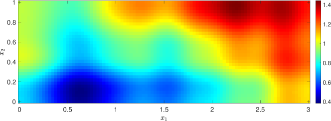
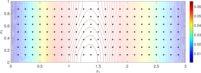
(a) The truth permeability (b) The pressure field and sensors

Figure 1: Test problem one setup ($L=2$).

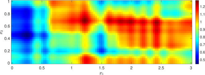
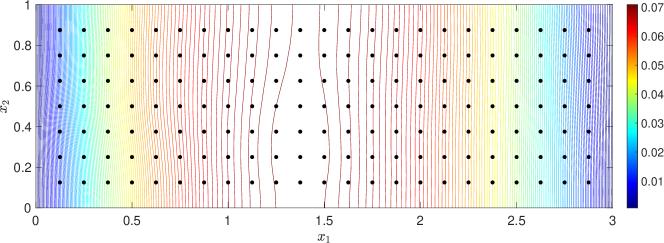
(a) The truth permeability (b) The pressure field and sensors

Figure 2: Test problem two setup ($L=1$).

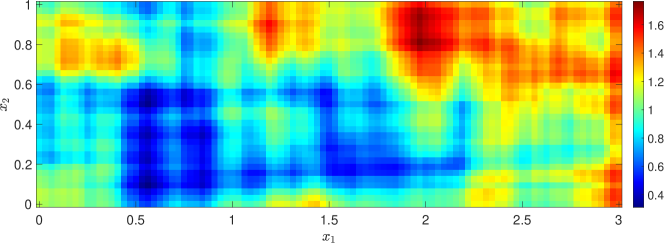
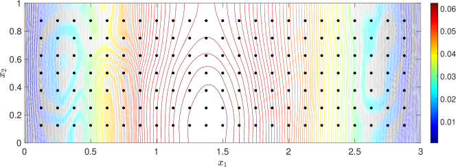
(a) The truth permeability (b) The pressure field and sensors

Figure 3: Test problem three setup ($L=0.5$).

For each subdomain $\mathcal{D}^{(i)}$ ($i=1,2,3$), the local KL expansion is computed (see (14)). To capture $95\%$ of the total variance for each subdomain, the number of local KL modes retained is $11$ for $L=2$, that is 33 for $L=1$ and that is $109$ for $L=0.5$ (as the subdomains have the same dimensionality, the numbers of their corresponding KL modes retained are the same for a given correlation length). The priori distributions of the local parameters $\{\xi_{r}^{(i)}\}_{r=1}^{d^{(i)}}$ (see (13)) for $i=1,2,3$ are set to be independent uniform distributions with range $I=[-1,1]$, and the support of $\xi^{(i)}$ is then $I_{\xi^{(i)}}=I^{d^{(i)}}$. For each local subdomain, the local problem (27) is discretized with the bilinear finite element method with a uniform $33\times 33$ grid (the number of the spatial degrees of freedom is 1089). All results of this paper are obtained in MATLAB on a workstation with 2.20 GHz Intel(R) Xeon(R) E5-2630 CPU. As solving the linear system associated with the global model (10) takes around $6.256\times 10^{-2}$ seconds and solving that associated with the local model (27) is around $3.845\times 10^{-3}$ seconds, we define the computational cost to conduct a local forward model evaluation as one cost unit, and consider the cost for each global model evaluation to be 16.25 cost units.

For comparison, the standard MCMC method (Algorithm 1) is applied with the global forward model (10), which is referred to as the global MCMC (G-MCMC) in the following. For both G-MCMC and our DD-MCMC (Algorithm 2), the proposal distribution (line 3 of Algorithm 1) is set to the symmetric Gaussian distribution, i.e., $Q(\xi^{\star}|\xi^{s})=\mathcal{N}(\xi^{s},\beta\bm{I})$ where $\bm{I}$ is an identity matrix and $\beta$ is the stepsize, which is specified for each test problem in Section 5.3. For test problem one ($L=2$), the number of posterior samples $N$ generated by DD-MCMC is set to $1\times 10^{4}$ (see line 19 of Algorithm 2); for test problem two ($L=1$), that is set to $2\times 10^{4}$; for test problem three ($L=0.5$), that is set to $4\times 10^{4}$. For a fair comparison, the number of posterior samples generated by G-MCMC is set to $1\times 10^{3}$, $2\times 10^{3}$ and $4\times 10^{3}$ for test problem one, test problem two and test problem three respectively, such that the costs of DD-MCMC and G-MCMC are approximately equal.

5.2 Results for the interface treatment

To construct GP models for the interface functions (discussed in Section 4.1), the test sets $\Delta^{(1,2)}$ and $\Delta^{(2,3)}$ (see line 7 of Algorithm 2) are set to the grid points on the interfaces, where each interface has $33$ grid points, and the threshold $\delta_{\text{tol}}$ for the maximum posterior variance (see line 10 of Algorithm 2) is set to $10^{-7}$. The maximum numbers of training data points required for the active learning procedure (i.e., $|\Lambda^{(i,j)}|$ for the last iteration step in line 13 of Algorithm 2) and the corresponding maximum posterior variance (i.e., $\sigma_{\Delta^{(i,j)}}^{\max}$ in line 9 of Algorithm 2 after the last iteration step) are shown in Table 1, where it can be seen that these numbers are small—at most five training data points are required to reach the desired threshold for the three test problems.

To assess accuracy of the interface treatment, we compute the difference between the GP interface models and the exact interface functions associated with the truth permeability fields of the three test problems. For each interface $\tau^{(i,j)}$, the relative interface error is computed through

$$\epsilon_{\text{int}}^{(i,j)}\mathrel{\mathop{\mathchar 58\relax}}=\|g^{(i,j)}(x,\xi)-\widetilde{g}^{(i,j)}(x)\|_{2}/\|g^{(i,j)}(x,\xi)\|_{2},$$

where $g^{(i,j)}(x,\xi)$ is the exact interface function defined as $g^{(i,j)}(x,\xi)\mathrel{\mathop{\mathchar 58\relax}}=u(x,\xi)|_{\tau^{(i,j)}}$ and $\widetilde{g}^{(i,j)}(x)$ is the trained GP interface model (see line 8 of Algorithm 2), and the parameter value $\xi$ is associated with each of the truth field. Moreover, for each local subdomain $\mathcal{D}^{(i)}$ ($i=1,2,3$), the relative state errors of local solutions obtained with the GP interface models are also assessed, which are computed through

$$\epsilon_{\text{state}}^{(i)}\mathrel{\mathop{\mathchar 58\relax}}=\|u_{\text{GP}}^{(i)}(x,\xi^{(i)})-u^{(i)}(x,\xi^{(i)})\|_{2}/\|u^{(i)}(x,\xi^{(i)})\|_{2}\,,$$

where $u_{\text{GP}}^{(i)}(x,\xi^{(i)})$ is the local solution defined in (27), $u^{(i)}(x,\xi^{(i)})$ is the exact local solution which is defined in (16), and $\xi^{(i)}$ is the local KL random variable (see (15)) associated with $\xi$. Table 2 shows the relative interface errors and state errors, where it can be seen that these errors are all very small.

Table 1: Maximum number of training data points and the correspoding maximum posterior variances for the three test problems.

$L$	$2$	$1$	$0.5$
$|\Lambda^{(1,2)}|$	4	4	4
$|\Lambda^{(2,3)}|$	4	4	5
$\sigma_{\Delta^{(1,2)}}^{\max}$	$3.979\times 10^{-13}$	$2.700\times 10^{-13}$	$4.105\times 10^{-9}$
$\sigma_{\Delta^{(2,3)}}^{\max}$	$1.856\times 10^{-10}$	$1.160\times 10^{-10}$	$7.555\times 10^{-9}$

Table 2: Relative errors for different interfaces

	$L$	$2$	$1$	$0.5$
$\epsilon_{\text{int}}$	$\tau^{(1,2)}$	$3.112\times 10^{-3}$	$3.825\times 10^{-3}$	$4.628\times 10^{-3}$
	$\tau^{(2,3)}$	$1.580\times 10^{-3}$	$1.925\times 10^{-3}$	$2.345\times 10^{-3}$
$\epsilon_{\text{state}}$	$\mathcal{D}^{(1)}$	$1.631\times 10^{-3}$	$1.728\times 10^{-3}$	$2.385\times 10^{-3}$
	$\mathcal{D}^{(2)}$	$2.743\times 10^{-4}$	$3.056\times 10^{-4}$	$4.455\times 10^{-4}$
	$\mathcal{D}^{(3)}$	$8.375\times 10^{-5}$	$1.083\times 10^{-4}$	$1.344\times 10^{-4}$

5.3 Performance of DD-MCMC

For the three test problems, values of the stepsize ($\beta$ is introduced in Section 5.1) are set as follows, such that the acceptance rate of DD-MCMC and G-MCMC is appropriate, which is defined by the number of accepted samples (line 7 of Algorithm 1) divided by the total sample size. For test problem one ($L=2$), the stepsize for DD-MCMC is set to $\beta=0.05$, and that for G-MCMC is set to $\beta=0.07$. For test problem two ($L=1$), that is set to $\beta=0.05$ for both DD-MCMC and G-MCMC. For test problem three ($L=0.5$), that is set to $\beta=0.05$ for DD-MCMC and $\beta=0.04$ for G-MCMC. Acceptance rates for the three test problems are shown in Table 3, which are consistent with the settings discussed in [41].

Table 3: Acceptance rates for the three test problems.

$L$	DD-MCMC			G-MCMC
	$\mathcal{D}^{(1)}$	$\mathcal{D}^{(2)}$	$\mathcal{D}^{(3)}$
2	48.73%	16.63%	15.97%	17.80%
1	42.10%	24.68%	12.51%	15.00%
0.5	47.73%	23.79%	19.37%	12.60%

Once samples of the posterior distributions are obtained, we compute the mean and variance estimates of the permeability fields as follows. For our DD-MCMC (Algorithm 2), the outputs are denoted by $\{\widehat{a}(x,\widehat{\xi}^{s})\}_{s=1}^{N}$ which are the posterior assembled fields (see (28)–(29)) to approximate the unknown permeability field. The corresponding mean and variance estimates are computed through

$$\check{\mathbb{E}}\left[\widehat{a}(x,\widehat{\xi})\right]\mathrel{\mathop{\mathchar 58\relax}}=\frac{1}{N}\sum_{s=1}^{N}\left[\widehat{a}(x,\widehat{\xi}^{s})\right],$$ (31)

$$\check{\mathbb{V}}\left[\widehat{a}(x,\widehat{\xi})\right]\mathrel{\mathop{\mathchar 58\relax}}=\frac{1}{N}\sum_{s=1}^{N}\left[\widehat{a}(x,\widehat{\xi}^{s})-\check{\mathbb{E}}[\widehat{a}(x,\widehat{\xi})]\right]^{2}.$$ (32)

For the local posterior samples $\{\xi^{(i),s},s=1,\ldots,N\}$ for $i=1,\ldots,M$ (corresponding to line 19 of Algorithm 2), the mean estimate of the local permeability field is obtained by putting samples of each local field (i.e. $\{a^{(i)}(x,\xi^{(i),s}),s=1,\ldots,N\}$ defined in (14)) into (31). Denoting the posterior samples of the stitched field as $\breve{a}(x,\xi^{s})\mathrel{\mathop{\mathchar 58\relax}}=\sum_{i=1}^{M}\widetilde{a}^{(i)}(x,\xi^{(i),s})$, where $\widetilde{a}^{(i)}(x,\xi^{(i),s})$ is the extension of the local field $a^{(i)}(x,\xi^{(i),s})$ following (17)–(18). The global mean and variance estimates based on the stitched field, denoted by $\check{\mathbb{E}}\left[\breve{a}(x,\xi)\right]$ and $\check{\mathbb{V}}\left[\breve{a}(x,\xi)\right]$ respectively, are obtained by putting the samples $\{\widetilde{a}^{(i)}(x,\xi^{(i),s}),s=1,\ldots,N\}$ into (31)–(32). Moreover, for samples $\{\xi^{s},s=1,\ldots,N\}$ generated by G-MCMC, the corresponding samples of the global permeability field are denoted by $\{a(x,\xi^{s}),s=1,\ldots,N\}$ (see (8)). The global mean and variance estimates, denoted by $\check{\mathbb{E}}\left[a(x,\xi)\right]$ and $\check{\mathbb{V}}\left[a(x,\xi)\right]$ respectively, are assessed through putting $\{a(x,\xi^{s}),s=1,\ldots,N\}$ into (31)–(32).

For the three test problems, Figure 4, Figure 5 and Figure 6 show the mean fields estimated using the samples obtained from DD-MCMC and G-MCMC. From Figure 4(a), Figure 5(a) and Figure 6(a), it is clear that the estimated field using the DD-MCMC outputs (the assembled fields $\{\widehat{a}(x,\widehat{\xi}^{s})\}_{s=1}^{N}$) are very similar to the truth permeability fields shown in Figure 1, Figure 2 and Figure 3. For test problem one where its truth permeability field is relatively smooth, although the sample mean of the assembled fields gives an accurate estimate (see Figure 4(a)), the sample mean of the stitched fields (i.e. $\{\breve{a}(x,\xi^{s}),s=1,\ldots,N\}$) gives misleading information on the interfaces (see Figure 4(b)). This is consistent with our analysis in Section 3.2, and confirms that our reconstruction procedure (line 21 of Algorithm 2) is necessary. The results associated with the stitched fields for test problem two and three are shown Figure 5(b) and Figure 6(b). It can be seen that as the truth permeability field of the underlying problem becomes less smooth, the effect of interface becomes less significant. However, it is still clear that the assembled fields give more accuracy mean estimates than the stitched fields. The results of G-MCMC are shown in Figure 4(c), Figure 5(c) and Figure 6(c), where it is clear that for a comparable computational cost, the estimated mean field from G-MCMC is less accurate than that of DD-MCMC (with the assembled fields). In addition, the estimated variance fields using the samples obtained from DD-MCMC and G-MCMC are shown in Figure 7, Figure 8 and Figure 9, where it can be seen that the variances are small.

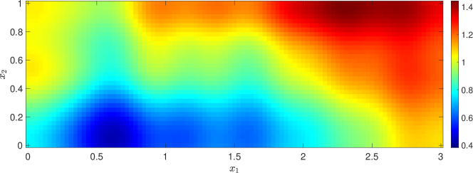
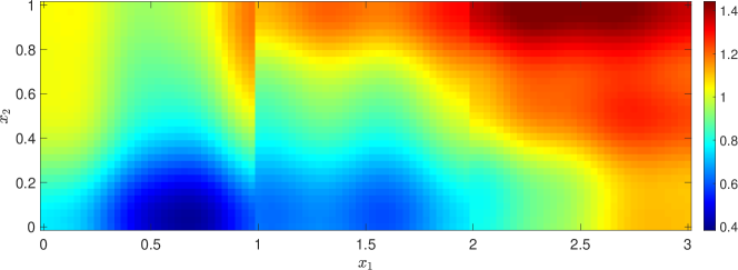
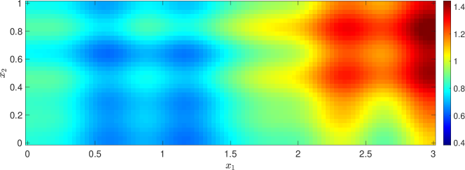
(a) Mean $\check{\mathbb{E}}\left[\widehat{a}(x,\widehat{\xi})\right]$, DD-MCMC (assembled). (b) Mean $\check{\mathbb{E}}\left[\breve{a}(x,\xi)\right]$, DD-MCMC (stitched). (c) Mean $\check{\mathbb{E}}\left[a(x,\xi)\right]$, G-MCMC.

Figure 4: Estimated mean fields for test problem one ($L=2$).

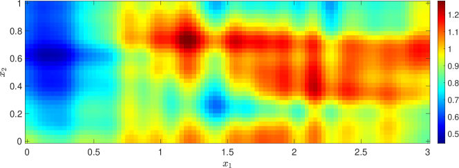
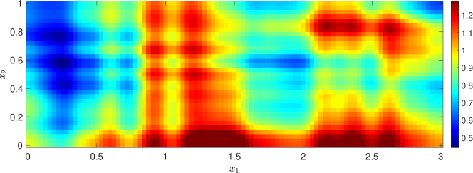
(a) Mean $\check{\mathbb{E}}\left[\widehat{a}(x,\widehat{\xi})\right]$, DD-MCMC (assembled). (b) Mean $\check{\mathbb{E}}\left[\breve{a}(x,\xi)\right]$, DD-MCMC (stitched). (c) Mean $\check{\mathbb{E}}\left[a(x,\xi)\right]$, G-MCMC .

Figure 5: Estimated mean fields for test problem two ($L=1$).

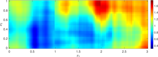
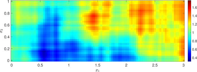
(a) Mean $\check{\mathbb{E}}\left[\widehat{a}(x,\widehat{\xi})\right]$, DD-MCMC (assembled). (b) Mean $\check{\mathbb{E}}\left[\breve{a}(x,\xi)\right]$, DD-MCMC (stitched). (c) Mean $\check{\mathbb{E}}\left[a(x,\xi)\right]$, G-MCMC.

Figure 6: Estimated mean fields for test problem three ($L=0.5$).

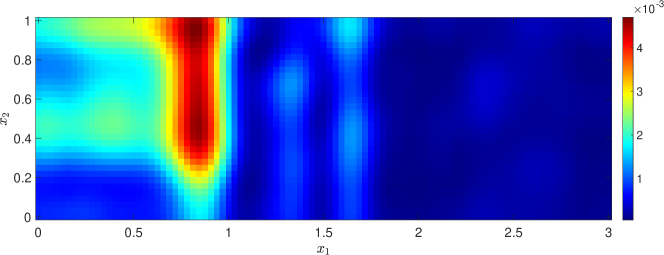
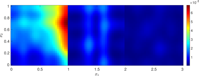
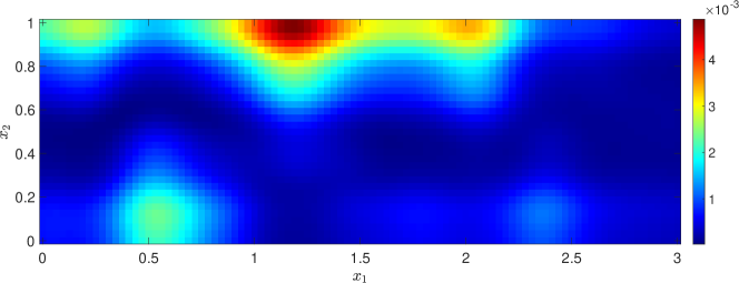
(a) Variance $\check{\mathbb{V}}\left[\widehat{a}(x,\widehat{\xi})\right]$, DD-MCMC (assembled). (b) Variance $\check{\mathbb{V}}\left[\breve{a}(x,\xi)\right]$, DD-MCMC (stitched). (c) Variance $\check{\mathbb{V}}\left[a(x,\xi)\right]$, G-MCMC.

Figure 7: Estimated variance fields for test problem one ($L=2$).

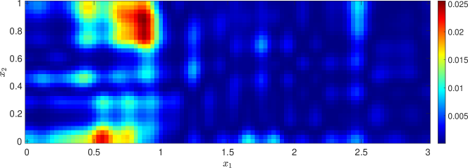
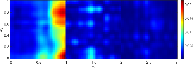
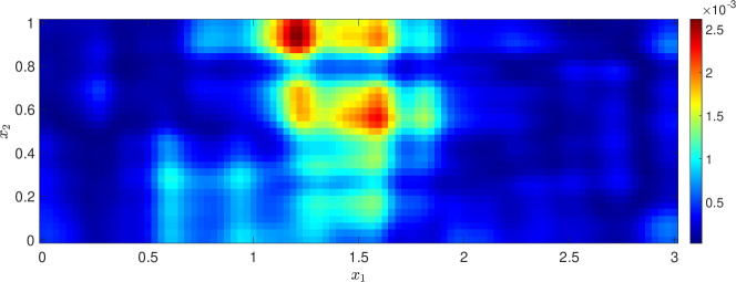
(a) Variance $\check{\mathbb{V}}\left[\widehat{a}(x,\widehat{\xi})\right]$, DD-MCMC (assembled). (b) Variance $\check{\mathbb{V}}\left[\breve{a}(x,\xi)\right]$, DD-MCMC (stitched). (c) Variance $\check{\mathbb{V}}\left[a(x,\xi)\right]$, G-MCMC.

Figure 8: Estimated variance fields for test problem two ($L=1$).

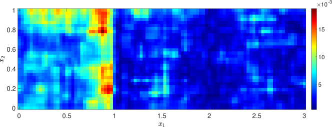
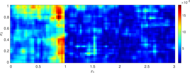
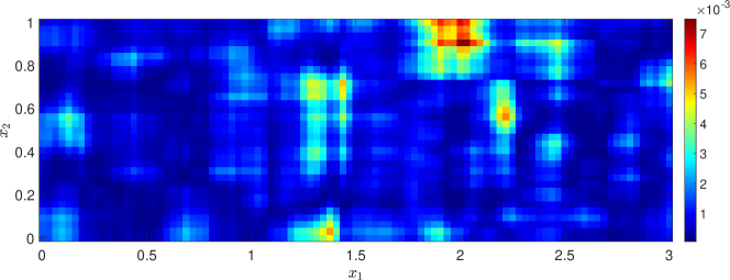
(a) Variance $\check{\mathbb{V}}\left[\widehat{a}(x,\widehat{\xi})\right]$, DD-MCMC (assembled). (b) Variance $\check{\mathbb{V}}\left[\breve{a}(x,\xi)\right]$, DD-MCMC (stitched). (c) Variance $\check{\mathbb{V}}\left[a(x,\xi)\right]$, G-MCMC.

Figure 9: Estimated variance fields for test problem three ($L=0.5$).

To assess the accuracy of the estimated posterior mean permeability, we introduce the following quantities of errors

$$\epsilon\mathrel{\mathop{\mathchar 58\relax}}=\|\check{\mathbb{E}}[a(x,\xi)]-a_{\text{truth}}\|_{2}/\|a_{\text{truth}}\|_{2},$$ (33)

$$\breve{\epsilon}\mathrel{\mathop{\mathchar 58\relax}}=\|\check{\mathbb{E}}[\breve{a}(x,\xi)]-a_{\text{truth}}\|_{2}/\|a_{\text{truth}}\|_{2},$$ (34)

$$\widehat{\epsilon}\mathrel{\mathop{\mathchar 58\relax}}=\|\check{\mathbb{E}}[\widehat{a}(x,\widehat{\xi})]-a_{\text{truth}}\|_{2}/\|a_{\text{truth}}\|_{2},$$ (35)

where $a_{\text{truth}}$ is the truth permeability, $\check{\mathbb{E}}[a(x,\xi)]$ is the mean estimate using the samples obtained from G-MCMC, $\check{\mathbb{E}}[\breve{a}(x,\xi)]$ is the mean estimate using the stitched fields obtained in DD-MCMC, and $\check{\mathbb{E}}[\widehat{a}(x,\widehat{\xi})]$ is the mean estimate using the assembled fields obtained in DD-MCMC. Table 4 shows these errors in the mean estimates for the three test problems. It is clear that the errors of our DD-MCMC (for both $\check{\mathbb{E}}[\widehat{a}(x,\widehat{\xi})]$ and $\check{\mathbb{E}}[\breve{a}(x,\xi)]$) are smaller than the errors of G-MCMC for the three test problems. In addition, the error for the stitched field ($\check{\mathbb{E}}[\breve{a}(x,\xi)]$) is slightly larger than that for the assembled field ($\check{\mathbb{E}}[\widehat{a}(x,\widehat{\xi})]$), which is consistent with our analysis discussed in Theorem 1.

Table 4: Errors in mean estimates for the three test problems.

$L$	$2$	$1$	$0.5$
$\widehat{\epsilon}$	$5.241\times 10^{-2}$	$7.928\times 10^{-2}$	$1.083\times 10^{-1}$
$\breve{\epsilon}$	$5.261\times 10^{-2}$	$8.571\times 10^{-2}$	$1.088\times 10^{-1}$
$\epsilon$	$1.340\times 10^{-1}$	$2.141\times 10^{-1}$	$1.805\times 10^{-1}$

6 Conclusion

The divide and conquer principle is one of the fundamental concepts to solve high-dimensional Bayesian inverse problems involving forward models governed by PDEs. With a focus on Karhunen-Loève (KL) expansion based priors, this paper proposes a domain-decomposed Markov chain Monte Carlo (DD-MCMC) algorithm. In DD-MCMC, difficulties caused by global prior fields with short correlation lengths are curbed through decomposing global spatial domains into small local subdomains, where correlation lengths become relatively large. On each subdomain, local KL expansion is conducted to result in relatively low-dimensional parameterization, and effective Gaussian process (GP) interface models are built with an active learning procedure. The global high-dimensional Bayesian inverse problem is then decomposed into a series of local low dimensional-problems, where the corresponding local forward PDE models are also significantly cheaper than the global forward PDE model. After that, MCMC is applied for local problems to generate posterior samples of the local input fields. With posterior samples of the local problems, a novel projection procedure is developed to reconstruct samples of the global input field, which are referred to as the assembled fields. Numerical results demonstrate the overall efficiency of the proposed DD-MCMC algorithm. As sufficient data are crucial for efficient Bayesian inversion, although domain decomposition can significantly reduce the computational costs for the inference procedure, small subdomains often only contain limited observation data, which limits the sizes of local subdomains. To further decompose the subdomains, a possible solution is to introduce new effective interface conditions with the whole observed data. Implementing such strategies will be the focus of our future work.

Acknowledgments: This work is supported by the National Natural Science Foundation of China (No. 12071291), the Science and Technology Commission of Shanghai Municipality (No. 20JC1414300) and the Natural Science Foundation of Shanghai (No. 20ZR1436200).

References

- [1] S. Springer, H. Harrio, J. Susiluoto, A. Bibov, A. Davis, Y. Marzouk, Efficient Bayesian inference for large chaotic dynamical systems, Geoscientific Model Development 14 (7) (2021) 4319–4333.
- [2] A. Solonen, P. Ollinaho, M. Laine, H. Haario, J. Tamminen, H. Järvinen, Efficient MCMC for climate model parameter estimation: parallel adaptive chains and early rejection, Bayesian Analysis 7 (3) (2012) 715–736.
- [3] J. Martin, L. C. Wilcox, C. Burstedde, O. Ghattas, A stochastic Newton MCMC method for large-scale statistical inverse problems with application to seismic inversion, SIAM Journal on Scientific Computing 34 (3) (2012) A1460–A1487.
- [4] H. Haario, M. Laine, M. Lehtinen, E. Saksman, J. Tamminen, Markov chain Monte Carlo methods for high dimensional inversion in remote sensing, Journal of the Royal Statistical Society: series B (statistical methodology) 66 (3) (2004) 591–607.
- [5] A. M. Stuart, Inverse problems: a Bayesian perspective, Acta numerica 19 (2010) 451–559.
- [6] J. Wang, N. Zabaras, A Bayesian inference approach to the inverse heat conduction problem, International Journal of Heat and Mass Transfer 47 (17) (2004) 3927–3941.
- [7] Y. Efendiev, T. Hou, W. Luo, Preconditioning Markov chain Monte Carlo simulations using coarse-scale models, SIAM Journal on Scientific Computing 28 (2) (2006) 776–803.
- [8] Y. M. Marzouk, H. N. Najm, L. A. Rahn, Stochastic spectral methods for efficient Bayesian solution of inverse problems, Journal of Computational Physics 224 (2) (2007) 560–586.
- [9] C. Lieberman, K. Willcox, O. Ghattas, Parameter and state model reduction for large-scale statistical inverse problems, SIAM Journal on Scientific Computing 32 (5) (2010) 2523–2542.
- [10] T. A. El Moselhy, Y. M. Marzouk, Bayesian inference with optimal maps, Journal of Computational Physics 231 (23) (2012) 7815–7850.
- [11] T. Bui-Thanh, O. Ghattas, J. Martin, G. Stadler, A computational framework for infinite-dimensional Bayesian inverse problems part I: The linearized case, with application to global seismic inversion, SIAM Journal on Scientific Computing 35 (6) (2013) A2494–A2523.
- [12] J. Li, Y. M. Marzouk, Adaptive construction of surrogates for the Bayesian solution of inverse problems, SIAM Journal on Scientific Computing 36 (3) (2014) A1163–A1186.
- [13] T. Cui, K. J. Law, Y. M. Marzouk, Dimension-independent likelihood-informed MCMC, Journal of Computational Physics 304 (2016) 109–137.
- [14] O. Zahm, T. Cui, K. Law, A. Spantini, Y. Marzouk, Certified dimension reduction in nonlinear Bayesian inverse problems, Mathematics of Computation 91 (336) (2022) 1789–1835.
- [15] C. Robert, G. Casella, Monte Carlo statistical methods, Springer Science & Business Media, 2013.
- [16] T. Cui, Y. M. Marzouk, K. E. Willcox, Data-driven model reduction for the Bayesian solution of inverse problems, International Journal for Numerical Methods in Engineering 102 (5) (2015) 966–990.
- [17] P. Chen, C. Schwab, Sparse-grid, reduced-basis Bayesian inversion, Computer Methods in Applied Mechanics and Engineering 297 (2015) 84–115.
- [18] L. Jiang, N. Ou, Multiscale model reduction method for Bayesian inverse problems of subsurface flow, Journal of Computational and Applied Mathematics 319 (2017) 188–209.
- [19] Q. Liao, J. Li, An adaptive reduced basis ANOVA method for high-dimensional Bayesian inverse problems, Journal of Computational Physics 396 (2019) 364–380.
- [20] R. G. Ghanem, P. D. Spanos, Stochastic finite elements: a spectral approach, Courier Corporation, 2003.
- [21] J. Li, A note on the Karhunen–Loève expansions for infinite-dimensional Bayesian inverse problems, Statistics & Probability Letters 106 (2015) 1–4.
- [22] L. Ellam, N. Zabaras, M. Girolami, A Bayesian approach to multiscale inverse problems with on-the-fly scale determination, Journal of Computational Physics 326 (2016) 115–140.
- [23] Y. Xia, N. Zabaras, Bayesian multiscale deep generative model for the solution of high-dimensional inverse problems, Journal of Computational Physics 455 (2022) 111008.
- [24] Y. Chen, J. Jakeman, C. Gittelson, D. Xiu, Local polynomial chaos expansion for linear differential equations with high dimensional random inputs, SIAM Journal on Scientific Computing 37 (1) (2015) A79–A102.
- [25] Q. Liao, K. Willcox, A domain decomposition approach for uncertainty analysis, SIAM Journal on Scientific Computing 37 (1) (2015) A103–A133.
- [26] A. A. Contreras, P. Mycek, O. P. Le Maître, F. Rizzi, B. Debusschere, O. M. Knio, Parallel domain decomposition strategies for stochastic elliptic equations. part a: Local Karhunen–Loève representations, SIAM Journal on Scientific Computing 40 (4) (2018) C520–C546.
- [27] A. A. Contreras, P. Mycek, O. P. Le Maître, F. Rizzi, B. Debusschere, O. M. Knio, Parallel domain decomposition strategies for stochastic elliptic equations part b: Accelerated Monte Carlo sampling with local PC expansions, SIAM Journal on Scientific Computing 40 (4) (2018) C547–C580.
- [28] S. Khajehpour, M. Hematiyan, L. Marin, A domain decomposition method for the stable analysis of inverse nonlinear transient heat conduction problems, International Journal of Heat and Mass Transfer 58 (1) (2013) 125–134.
- [29] A. D. Jagtap, E. Kharazmi, G. E. Karniadakis, Conservative physics-informed neural networks on discrete domains for conservation laws: Applications to forward and inverse problems, Computer Methods in Applied Mechanics and Engineering 365 (2020) 113028.
- [30] A. D. Jagtap, G. E. Karniadakis, Extended physics-informed neural networks (XPINNs): A generalized space-time domain decomposition based deep learning framework for nonlinear partial differential equations, Communications in Computational Physics 28 (5) (2020) 2002–2041.
- [31] K. Shukla, A. D. Jagtap, G. E. Karniadakis, Parallel physics-informed neural networks via domain decomposition, Journal of Computational Physics 447 (2021) 110683.
- [32] M. Ainsworth, J. Oden, A posteriori error estimation in finite element analysis, Wiley, 2000.
- [33] H. Elman, D. Silvester, A. Wathen, Finite Elements and Fast Iterative Solvers: with Applications in Incompressible Fluid Dynamics, Oxford University Press (UK), 2014.
- [34] N. Metropolis, A. W. Rosenbluth, M. N. Rosenbluth, A. H. Teller, E. Teller, Equation of state calculations by fast computing machines, The journal of chemical physics 21 (6) (1953) 1087–1092.
- [35] W. K. Hastings, Monte Carlo sampling methods using Markov chains and their applications, Biometrika 57 (1) (1970) 97 – 109.
- [36] O. Le Maître, O. M. Knio, Spectral methods for uncertainty quantification: with applications to computational fluid dynamics, Springer Science & Business Media, 2010.
- [37] A. M. Quarteroni, A. Valli, Domain decomposition methods for partial differential equations, Oxford University Press, 1999.
- [38] C. E. Rasmussen, C. K. Williams, Gaussian process for machine learning, The MIT Press, 2006.
- [39] C. E. Rasmussen, H. Nickisch, Gaussian processes for machine learning (GPML) toolbox, The Journal of Machine Learning Research 11 (2010) 3011–3015.
- [40] D. Silvester, H. Elman, A. Ramage, Incompressible Flow and Iterative Solver Software (IFISS) version 3.5, http://www.manchester.ac.uk/ifiss/ (September 2016).
- [41] G. O. Roberts, J. S. Rosenthal, Optimal scaling for various Metropolis-Hastings algorithms, Statistical science 16 (4) (2001) 351–367.