Missing data interpolation in integrative multi-cohort analysis with disparate covariate information

Abstract

Integrative analysis of datasets generated by multiple cohorts is a widely-used approach for increasing sample size, precision of population estimators, and generalizability of analysis results in epidemiological studies. However, often each individual cohort dataset does not have all variables of interest for an integrative analysis collected as a part of an original study. Such cohort-level missingness poses methodological challenges to the integrative analysis since missing variables have traditionally: (1) been removed from the data for complete case analysis; or (2) been completed by missing data interpolation techniques using data with the same covariate distribution from other studies. In most integrative-analysis studies, neither approach is optimal as it leads to either loosing the majority of study covariates or challenges in specifying the cohorts following the same distributions. We propose a novel approach to identify the studies with same distributions that could be used for completing the cohort-level missing information. Our methodology relies on (1) identifying sub-groups of cohorts with similar covariate distributions using cohort identity random forest prediction models followed by clustering; and then (2) applying a recursive pairwise distribution test for high dimensional data to these sub-groups. Extensive simulation studies show that cohorts with the same distribution are correctly grouped together in almost all simulation settings. Our methods’ application to two ECHO-wide Cohort Studies reveals that the cohorts grouped together reflect the similarities in study design. The methods are implemented in R software package relate. Missing data; Meta analysis; Data integration; Random forest; Clustering; Distribution similarity.

1 Introduction

Collaborative study designs (CSD) in which individual data from multiple independent contributing studies (ICS) have become more common (Lesko and others, 2018). The advantages of combining data from multiple sources include increased statistical power through larger sample sizes, increased potential for investigating effect heterogeneity, and increased value by capitalizing on resources already used by the existing studies. However, despite numerous examples of CSDs (Table 1 in Lesko and others, 2018) the issue of missing data interpolation at the study level has not been a focus of much research.

The ECHO-wide Cohort Study harmonizes extant data from 69 ongoing ICS across the U.S. to study environmental factors associated with child health. Each of these ICS were initiated with heterogeneity in the research design due to the each of their overall research goals. Thus, the extant data that has been collected may have been done with different “tools” (i.e., questionnaires, assays, etc.) and may or may not have overlapping data elements with the other studies being pooled to form the ECHO-wide Cohort. While the collected data have now been harmonized, the analysis of these extant data still creates an issue of how to deal with missingness at the ICS level. For example, if we have a causal question about an exposure, $X$ on $Y$, we need data on all the potential confounders to have the assumption of exchangeability hold. Yet, if among the 69 cohorts, only a subset have the full set of confounding variables, it is unclear how to handle this missingness. The potential options include (but not limited to): (1) do a complete case analysis and drop the ICS that have not collected the full set of potential confounders; (2) pool all the data, conduct imputation, and ignore the issue that each of the ICS likely represent different populations and therefore the joint distributions may be heterogeneous between cohorts; or, (3) impute by grouping ICS into subsets based upon some meta-level information such as who, how, and when individuals were recruited into each of the studies. This last part is difficult as it is not always clear how the samples are different. Additionally, as multiple imputation relies on the joint distribution of the variables pertinent to the analyses, one may erroneously group ICS together when they should not be and vice versa (Azur and others (2011)).

The question of cohort-level missing data inference in CSD has been discussed by Kundu and others (2019) in the context of regression modeling of an outcome given a set of covariates. However, these methods assume the similarity in distribution of covariates across all studies, which, in practice, often may not hold. We consider an alternative approach in which imputation is based on clusters that suggest that the joint distribution of the observed data is not different from one another. Therefore, we propose an approach that clusters the ICS based upon the joint distribution of the pertinent variables that are observed. This is analogous to assuming that the data are missing at random (MAR) given the joint distribution of observed pertinent variables (Rubin, 1976; Little and Rubin, 2019). The approach we consider is a two-stage approach, where we first identify groups by the joint distribution of observed variables, and then utilize imputation to account for the ICS level missing covariates. This approach is computationally feasible over directly testing all pairwise ICS comparisons which would be a brute force approach that in large collaborative studies becomes increasingly computationally expensive especially when each of the ICS has increasingly larger sample size.

2 Methods

We introduce a novel approach for identifying sub-groups of cohorts with the same joint distribution on the measured covariates for use in pooled individual data analyses to allow ICS-level missing data interpolation. We start by introducing some notation. We assume there are $K$ ICS, which for simplicity we assume are all of a cohort study design. We denote individuals within each cohort $i=1,\dots,I_{k},k=1,\dots,K$. Suppose that for each individual we observe a set of variables $\boldsymbol{z}_{ik}=\{z_{pik}\}_{p=1}^{P}$ of length $P$, which combines all measures of interest for a CSD analysis and may include an outcome, exposures, confounders, and effect modifiers (see Figure 1). We further assume that the data for a sub-set of variables $J\subset\{1,2,\dots,P\}$ is either not collected by at least one study or has a large percentage of missing data, which would make cohort-level interpolation statistically inappropriate.

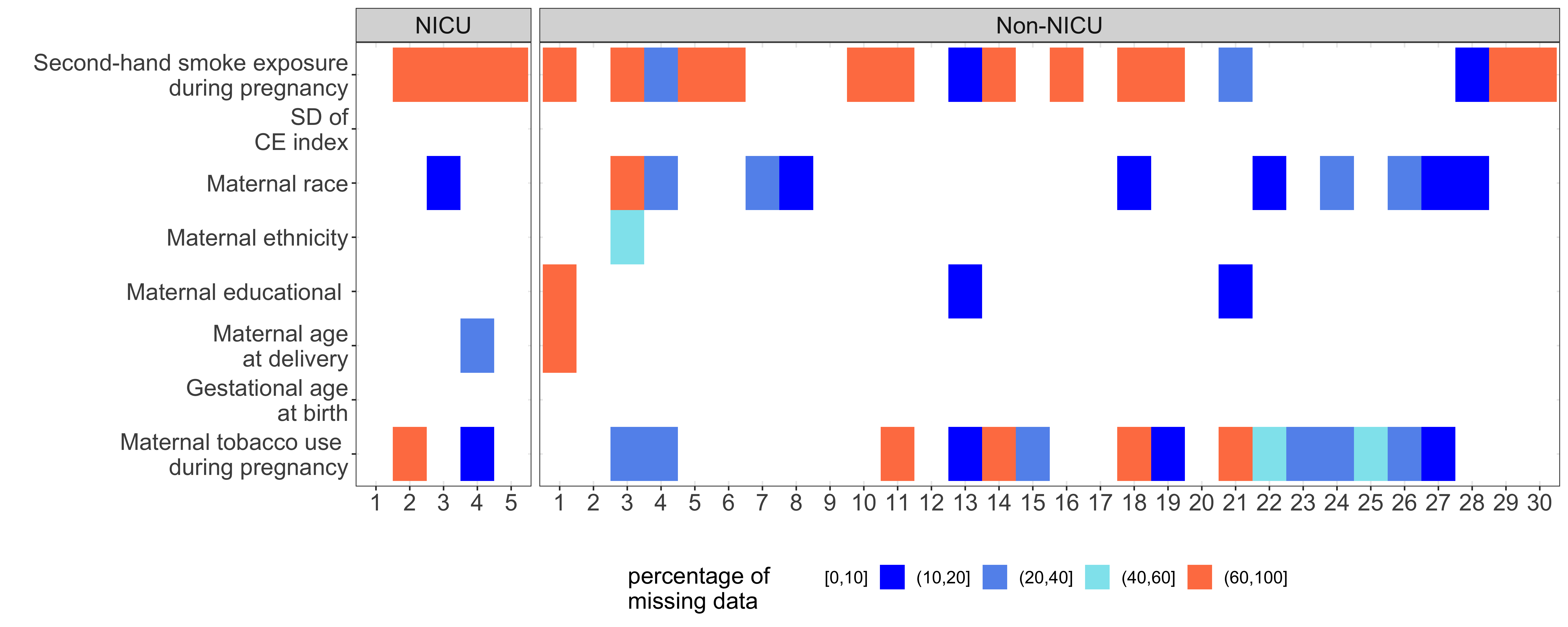
Figure 1: Missing data pattern for the Neighborhood-level exposures to environmental and social stressors on pre-term birth study Martenies and others (2022). The color scale represents the proportion of missing covariates (y-axis) for each cohort (x-axis). Cohorts are grouped by corresponding study design: (1) NICU - children who stayed at neonatal intensive care unit; (2) non-NICU - all other children.

We consider a two-stage approach called REcursive muLtivariAte TEsting for cohort clustering (relate), where we first (1) identify sub-groups of cohorts based on their similarity in the variables $\boldsymbol{z}_{ik}$ of interest for the CSD analysis and then (2) formally test the equivalence in distributions for these sub-groups. Our sub-grouping approach substantially reduces the number of tests needed for the distributional equivalence and the corresponding computational time. The full procedure is summarized in Algorithm 1.

Data: Participant-level table with covariates for meta-analysis $\boldsymbol{z}_{ik}$ and cohort membership ID ($k=1,\dots,K$); significance level $\alpha$

Result: Cohort groups with same distribution on pooled data covariates

Stage 1: Identifying sub-groups of cohorts with similar distributions

Step 1: Random forest classification;

      (i) Run multi-class random forest model to predict cohort ID using pooled data analysis covariates as predictors;

      (ii) Calculate pairwise random forest distance between participant-level observations;

      (iii) Average participant-level pairwise random forest distance within each cohort;

Step 2: Clustering to identify sub-groups of similar cohorts;

      (i) Run hierarchical clustering algorithm on cohort-level random forest distance matrix;

      (ii) Extract clustering dendrogram (D) to identify cohorts that group together;

Stage 2: Recursive pairwise distribution test for high dimensional data

Biswas and Ghosh (BG) procedure on clustering dendrogram to test cohort similarity.

Algorithm 1 Cohort subgroups identification.

2.1 First stage—identifying sub-groups of cohorts with similar distributions

We start measuring the cohort similarity using a multi-class random forest model. Specifically, given a vector of $\boldsymbol{z}_{ik}$ measures over a total of $KI_{k}$ observations in $K$ studies, we build a random forest model to predict the cohort membership, $k=1,\dots,K$All covariates of interest for the pooled analysis are used as predictors in the random forest model, where cohort-level missing covariates are interpolated within the model using the random forest imputation (na.action="na.impute" option in R function rfsrc). In this approach, the model decision tree, $\mathcal{T}_{b}$, is built for each bootstrap sample $\mathcal{I}_{b}\subset\{1,\dots,KI_{k}\}$ of observations, where $~{}b=1,\dots,B$.

To model the similarity between the cohorts based on their covariate distribution, we propose to use the random forest proximity measures. Random forest proximity can then be calculated using the measures of closeness between two observations on the decision tree $\mathcal{T}_{b}$ and averaged across $B$ trees (Breiman, 2003). The traditional random forest proximity measures the frequency at which two observations end up in the same terminal node of the decision tree $\mathcal{T}_{b}$. However, this proximity does not account for the tree hierarchical structure and two observations from different nodes are treated equivalently regardless of the split location (Mantero and Ishwaran, 2021). To overcome this drawback, we utilize the random forest dissimilarity introduced by Mantero and Ishwaran (2021) that counts the number of splits on the tree path between a pair of observations $\boldsymbol{z}_{ik}$ and $\boldsymbol{z}_{jl}$ terminal nodes. Formally, let $S(\boldsymbol{z}_{ik},\boldsymbol{z}_{jl},\mathcal{T}_{b})$ be the the minimum number of splits on the path from the terminal node containing $\boldsymbol{z}_{ik}$ to the terminal node containing $\boldsymbol{z}_{jl}$ in $\mathcal{T}_{b}$ such that the path includes at least one common ancestor node of $\boldsymbol{z}_{ik}$ and $\boldsymbol{z}_{jl}$. Let $R(\boldsymbol{z}_{ik},\boldsymbol{z}_{jl},\mathcal{T}_{b})$ be the the minimum number of splits on the path from the terminal node containing $\boldsymbol{z}_{ik}$ to the terminal node containing $\boldsymbol{z}_{jl}$ in $\mathcal{T}_{b}$ such that the path includes the root node. Then the random forest dissimilarity measure between $\boldsymbol{z}_{ik}$ and $\boldsymbol{z}_{jl}$ is given by

$$d_{ik,jl}=D(\boldsymbol{z}_{ik},\boldsymbol{z}_{jl})=\frac{1}{B}\sum_{b=1}^{B}\frac{S(\boldsymbol{z}_{ik},\boldsymbol{z}_{jl},\mathcal{T}_{b})}{R(\boldsymbol{z}_{ik},\boldsymbol{z}_{jk},\mathcal{T}_{b})}.$$ (1)

To identify the sub-groups of cohorts with similar distributions, we first calculate the distance matrix with pair-wise random forest dissimilarity (1) between observations $D=\{d\}_{ik,jl}$, where $i=1,\dots,I_{k}$ are the individuals within cohort $k$ and $j=1,\dots,I_{l}$ are the individuals within cohort $l$; $k,l=1,\dots,K$. We then average these distances across all observations within the same cohort to obtain pair-wise random forest dissimilarity between cohorts, $\bar{D}=\{\bar{d}\}_{k,l}$, such that

$$\bar{d}_{k,l}=D(\boldsymbol{z}_{k},\boldsymbol{z}_{l})=\frac{1}{I_{k}}\frac{1}{I_{l}}\sum_{i=1}^{I_{k}}\sum_{j=1}^{I_{l}}D(\boldsymbol{z}_{ik},\boldsymbol{z}_{jl}).$$ (2)

The cohort-level pairwise distance matrix is then used in hierarchical clustering algorithm to group the cohorts (Legendre and Legendre, 2012; Gordon, 1999). This hierarchical dendrogram is used to guide the second stage and reduce the number of pairwise comparisons.

Our approach assumes that observations in two or more distinct cohorts that come from the same distribution will fall close on the random forest decision tree and thus will have smaller dissimilarity measure as opposed to the variables that come from the different distributions. Specifically, for all $i,j$ we expect $d_{ik,jl}$ to be small if cohorts $k$ and $l$ have the same distribution and large if cohorts $k$ and $l$ come from different distributions. Averaging random distances across all observations within the same cohort is necessary to characterize dissimilarities at the cohort level that is of interest for the current study. Finally, the clustering step allows to efficiently identify the similarity structure between the cohorts by constructing a hierarchical dendrogram.

2.2 Second stage—recursive pairwise distribution test for high dimensional data

The first stage of the proposed algorithm identifies the hierarchical similarity structure among the cohorts with a goal of reducing the number of tests required to formally test for the equivalence of multivariate distributions in the second stage. This is done by applying the two-sample non-parametric test for the multi-variate distributional equivalence developed by Biswas and Ghosh (BG) (Biswas and Ghosh, 2014). We recursively apply the BG test according to the clustering dendrogram. This non-parametric test is designed for testing the equivalence of two distributions $F$ and $G$ (not necessarily Gaussian) by comparing the average Euclidean distances between the samples from these distributions. Formally, consider the independent random vectors $\boldsymbol{X},\boldsymbol{X}_{*}\overset{iid}{\sim}F$ and $\boldsymbol{Y},\boldsymbol{Y}_{*}\overset{iid}{\sim}G$. Let $D_{FF}$, $D_{GG}$ and $D_{FG}$ be the distributions of Euclidean distances between random vectors $\|\boldsymbol{X}-\boldsymbol{X}_{*}\|$, $\|\boldsymbol{Y}-\boldsymbol{Y}_{*}\|$, $\|\boldsymbol{X}-\boldsymbol{Y}\|$, respectively, and $\mu_{FF}$, $\mu_{GG}$, $\mu_{FG}$ their means. Let bivariate vectors $(\|\boldsymbol{X}-\boldsymbol{X}_{*}\|,\|\boldsymbol{X}-\boldsymbol{Y}\|)$ and $(\|\boldsymbol{Y}-\boldsymbol{Y}_{*}\|,\|\boldsymbol{X}-\boldsymbol{Y}\|)$ follow distributions $D_{F}$ and $D_{G}$, respectively, and $\mu_{D_{F}}$, $\mu_{D_{G}}$ be their respective means. Then if $F$ and $G$ differ, so do $D_{F}$ and $D_{G}$, and visa versa. Therefore, instead of testing $H_{0}:F=G$, the equivalent null hypothesis $H_{0}:\mu_{D_{F}}=\mu_{D_{G}}$ is tested. The corresponding test statistic is calculated from the samples $\boldsymbol{x}_{1},\dots,\boldsymbol{x}_{m}\overset{iid}{\sim}F$ and $\boldsymbol{y}_{1},\dots,\boldsymbol{y}_{n}\overset{iid}{\sim}G$ as

$$\hat{\mu}_{D_{F}}=\Big{[}\hat{\mu}_{FF}={m\choose 2}^{-1}\sum_{i=1}^{m}\sum_{j=i+1}^{m}\|\boldsymbol{x}_{i}-\boldsymbol{x}_{j}\|;\hat{\mu}_{FG}=(mn)^{-1}\sum_{i=1}^{m}\sum_{j=1}^{n}\|\boldsymbol{x}_{i}-\boldsymbol{y}_{j}\|\Big{]}$$ (3)

$$\hat{\mu}_{D_{G}}=\Big{[}\hat{\mu}_{FG}=(mn)^{-1}\sum_{i=1}^{m}\sum_{j=1}^{n}\|\boldsymbol{x}_{i}-\boldsymbol{y}_{j}\|;\hat{\mu}_{GG}={n\choose 2}^{-1}\sum_{i=1}^{n}\sum_{j=i+1}^{n}\|\boldsymbol{y}_{i}-\boldsymbol{y}_{j}\|\Big{]}.$$

An example of this procedure for the case of testing distributional similarity among $K=10$ simulated cohorts is schematically represented in Figure 2. Let the data from cohorts $1,2,\dots,10$ follow distributions $F_{1},F_{2},\dots,F_{10}$, respectively. Note that each of the distributions within the following sets are from the same underlying distribution: {$F_{1},F_{2},F_{3}$}, $\{F_{4},F_{5},F_{6}\}$, and $\{F_{7},F_{8},F_{9},F_{10}\}$. We start by applying the BG test (3) to the data at the same height on the terminal nodes of the dendrogam. Specifically, the following null hypotheses are tested:

$$H_{0}^{1}:F_{2}=F_{3};~{}H_{0}^{2}:F_{4}=F_{6};~{}H_{0}^{3}:F_{9}=F_{10};~{}H_{0}^{4}:F_{7}=F_{9};~{}H_{0}^{5}:F_{7}=F_{10}.$$ (4)

If null hypotheses $H_{0}^{1},\dots,H_{0}^{5}$ are not rejected at the pre-specified $\alpha$-level, then corresponding cohorts (1) $2$ and $3$; (2) $4$ and $6$; (3) $9$ and $10$; (4) $7$ and $9$; (5) $7$ and $10$ have same distributions and are combined in further analysis. If either $H_{0}$ were rejected, then corresponding cohorts have different distributions and no further testing is performed. For the combined data, the algorithm then moves to the next height of the dendrogram and the following hypotheses are tested

$$H_{0}^{6}:F_{2,3}=F_{1};~{}H_{0}^{7}:F_{4,6}=F_{5};~{}H_{0}^{8}:F_{7,9,10}=F_{8},$$ (5)

where $F_{2,3}$, $F_{4,6}$ and $F_{7,9,10}$ are the distributions of the combined cohorts (a) $2$ and $3$, (b) $4$ and $6$, (c) $7$, $9$, and $10$, respectively. The procedure is repeated until the cohorts’ similarity is tested at the higher heights of the dendrogram, and so on until either the test rejects the null hypothesis and we stop grouping cohorts or all cohorts are combined.

For each comparison using the BG test, the distribution being tested is on the overlapping observed variables. Therefore, each comparison at the first level of the dendrogram may be on different subsets of the $P$ variables. However, once two cohorts have been combined there are two different options for comparing a set of combined cohorts against a cohort at a higher level of the dendrogram (e.g., $H_{0}^{8}:F_{7,9,10}=F_{8}$). The first option is to only keep the comparison in the BG test to the overlapping variables and non-missing data even if for instance a missing variable in cohort 9 could be imputed due to combining with cohorts 7 and 10. The second approach is to impute the cohort level missing variable in cohort 9 by utilizing the information of the joint distributions of cohorts 7 and 10 with the non-missing variables in cohort 9. Provided that the assumption of the procedure is: given the observed variables, we cannot reject the null hypotheses of $H_{0}^{3}$, $H_{0}^{4}$, and $H_{0}^{5}$. We evaluate the accuracy of both approaches in Simulation section.

Additionally, in following our approach (see Algorithm S1 in the Supplementary Materials), there is the possibility that a cohort could be considered to be able to fit into two different clusters. Using the prior example, let us assume that the null hypotheses $H_{0}^{3}$ and $H_{0}^{5}$ were not rejected but $H_{0}^{4}$ was rejected at the $\alpha$-level. This would suggest that cohort 10 could be combined with either cohort 7 or with cohort 9, but cohort 7 and 9 are different enough from one another by the BG test and thus forming 2 clusters at this time point. The decision at this point is how to combine cohort 10 with either cohort 7 or cohort 9. We prioritize combining cohorts in this situation by the BG test statistic or equivalently by the magnitude of the p-value. The higher the p-value the closer the two cohorts are to one another. Therefore if the p-value for $H_{0}^{3}$ was $0.89$ and for $H_{0}^{5}$ was $0.41$ then cohort 10 would be combined with cohort 9 under this prioritization rule.

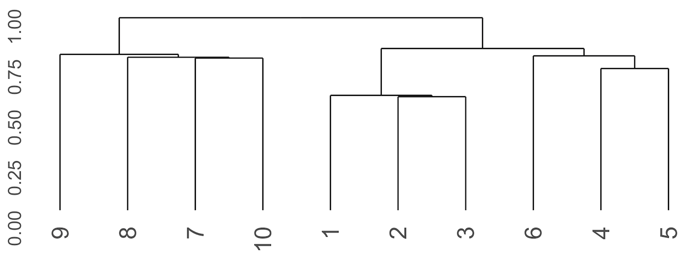
Figure 2: Example clustering dendrogram for the cohort similarity testing. The numerical labels on the dendrogram terminal nodes correspond to the individual cohorts identification numbers.

3 Simulation study

3.1 Simulation settings

To evaluate the ability of the proposed relate method to detect cohorts with similar distributions, we simulate 10 cohorts with 15 covariates in each. For each simulation, the sample size of each cohort is randomly selected from the set $\{30,50,100,200,500,700,750,900,1000,1200\}$. The distribution of the covariates is as follows: 10 covariates follow a multivariate normal distribution, two covariates are binary (above versus below the median of the normal distribution), one covariate is binomial, and the last two covariates are multinomial. Using these settings, we tested the following five simulation cases with 100 simulation per each scenario:

Case 1: same distribution. Cohorts 1-10 are generated from one set of distribution parametersfor each type of distribution.
Case 2: two distributions. Cohorts 1-8 and 9-10 are generated using two sets of parameters for each type of distribution, where for the normally distributed covariates the two parameter sets have different means but the same covariance.
Case 3: three distributions. Cohorts 1-8, 4-6, and 7-10 are generated using three sets of parameters for each type of distribution, where for the normally distributed covariates the three parameter sets have different means but the same covariance.
Case 4: two distributions. Cohorts 1-5 and 6-10 are generated using two sets of parameters for each type of distribution, where for the normally distributed covariates the two parameter sets have different means but the same covariance.
Case 5: four distributions. Cohorts 1-3, cohorts 4 and 5, cohorts 6 and 7, and cohorts 8-10 are generated using four sets of parametersfor each type of distribution, where for the normally distributed covariates the two parameter sets have different means and different covariance.
The distribution parameters for each simulation case are summarized in Table S1 in the Supplementary Materials.

To mimic the ECHO data, we add a layer of missing at random (MAR), where four cohorts are missing four covariates, with a percentage of 40%, and 60% of data missing in these covariates, respectively. Next, we randomly choose the number of cohort-level missing covariates according to the following scenarios: (Scenario 1) 2 cohorts missing 2 covariates; (Scenario 2) 2 cohorts missing 4 covariates; (Scenario 3) 5 cohorts missing 2 covariates; (Scenario 4) 5 cohorts missing 4 covariates; (Scenario 5) 5 cohorts missing 6 covariates. These numbers are chosen to examine the low (scenario 1-2), medium (scenario 3), and high (scenario 4-5) levels of missingness. These scenarios are chosen to quantify the potential decrease of the proposed relate method performance with increasing missingness level.

3.2 Simulation results

The performance of the relate method is evaluated based on the following metrics: (1) correct number of detected cohort clusters, which corresponds to the number of distributions in each simulation scenario; (2) the number of cohorts assigned to the wrong cluster of distributions, which counts whether the cohorts assigned to the same cluster originate from the same distribution; (3) the time (in seconds) to fit the random forest model and hierarchical clustering; (4) the time to conduct the BG test per simulation. all simulations were performed on a cluster with 128GB-512GB per node RAM (https://bit.ly/VCUCluster).

The results for all simulation scenarios are summarized in Tables 1 and 2 for the case without and with missing data imputation at each step of recursive BG test, respectively. When recursive pairwise distribution BG test is performed without interpolating missing data for the cohorts that are combined at each step of recursion, the overall accuracy of the relate method is substantially higher. Specifically, relate identifies clusters of same distributions with over $90\%$ accuracy for the first 4 simulation cases with $1$ to $3$ different distribution clusters in $10$ simulated cohorts. As expected, the accuracy is overall lower when the missingness level increases. The number of correctly identified clusters is lower for simulation case $5$, where data from $4$ different distributions is generated. The performance of this method for this simulation case is especially low ($54\%$ accuracy) when the number of cohort-level missing covariates is high. This low performance may be explained by the low number of cohorts with similar distribution in each cluster ($2$ to $3$).

When missing data is imputed at each step of the recursive BG test algorithm, relate method identifies the clusters of similar distributions with over $99\%$ accuracy if there are $2$ cohort-level missing variables and up to a four distinct distributions. With the larger number of missing variables, the number of cohort clusters increase which leads to the lower number of correctly defined distribution clusters. It should be noted that the rate for the wrong number of assignments is low, which means that similar distributions are combined correctly but a large cluster of similar distributions may be split into two or more distinct clusters. However, with four distinct distributions out of the 10 cohorts, some cohorts are combined into incorrect clusters in $23-27\%$ of all simulation cases except for the case with five cohorts missing two covariates.

The average running time for the stage 1 (random forest and clustering method) of approach is approximately 50 seconds, and the average time for stage 2 (BG testing for similarity in distributions) is approximately 40 seconds. Together, these results indicate that the proposed relate methodology accurately detects clusters of similar distributions even when multiple cohorts are missing a large number of covariates. The run time for the method is on average under 2 minutes, which makes it feasible to implement on large-scale data sets.

Table 1: Performance summary of relate without imputation while running BG test by each cohort-level covariate missingness scenario and the true number of distribution clusters over 100 simulations. Results are summarized by (1) correct number of detected cohort clusters; (2) the number of cohorts assigned to the wrong cluster of distributions; (3) the time (in seconds) to fit the random forest model and hierarchical clustering; (4) the time to conduct the BG test per simulation.

Scenario	Number	Number	Sim	Number of	Number of	Number of	% of	Time/sim
	of	of	Case	Correct	Wrong	Correct	Wrong	RF	BG
	Cohorts	Covariates		Clusters	Clusters	Assignments	Assignments
1	2	2	1	100	0	0	100	49.07	38.97
			2	100	0	0	100	60.75	49.42
			3	100	0	0	100	51.75	33.27
			4	100	0	0	100	57.28	15.89
			5	98	2	29	71	32.9	12.82
2	2	4	1	100	0	0	100	49.9	71.60
			2	100	0	0	100	43.5	52.22
			3	100	0	0	100	38.7	11.84
			4	100	0	0	100	41.14	15.43
			5	87	13	46	54	36.02	13.35
3	5	2	1	100	0	0	100	49.97	71.60
			2	100	0	0	100	43.54	52.22
			3	100	0	0	100	38.71	11.84
			4	100	0	0	100	41.24	27.72
			5	98	2	21	79	42.24	16.66
4	5	4	1	100	0	0	100	51.70	83.01
			2	100	0	0	100	49.93	136.83
			3	98	2	6	94	43.17	18.68
			4	100	0	0	100	45.36	47.32
			5	98	2	21	79	42.44	16.66
5	5	6	1	100	0	0	100	87.14	79.79
			2	99	1	1	99	81.72	88.30
			3	98	2	9	91	53.79	14.15
			4	100	0	0	100	53.67	22.40
			5	90	10	46	54	52.06	14.29

Table 2: Performance summary of relate with imputation while running BG test by each cohort-level covariate missingness scenario and the true number of distribution clusters over 100 simulations. Results are summarized by (1) correct number of detected cohort clusters; (2) the number of cohorts assigned to the wrong cluster of distributions; (3) the time (in seconds) to fit the random forest model and hierarchical clustering; (4) the time to conduct the BG test per simulation.

Scenario	Number of	Number of	Simulation	Number of	Number of	Time/sim
(Missingness	Missing	Missing	Case	Correct	Wrong	—
level)	Cohorts	Covariates		Clusters	Clusters	RF	BG
1	2	2	1	100	0	49.07	53.50
			2	100	0	60.75	63.54
			3	98	1	51.77	24.53
			4	99	0	57.28	24.77
			5	100	25	32.96	21.69
2	2	4	1	81	0	49.97	73.79
			2	91	0	43.54	61.85
			3	68	2	38.71	19.00
			4	77	0	41.14	22.31
			5	84	27	36.02	20.55
3	5	2	1	96	0	47.25	73.71
			2	96	0	46.29	83.38
			3	100	0	38.49	22.19
			4	100	0	41.24	27.72
			5	100	1	37.39	21.92
4	5	4	1	68	0	51.70	119.92
			2	65	0	49.93	133.43
			3	85	1	43.17	39.93
			4	68	0	45.36	69.29
			5	95	6	42.44	25.84
5	5	6	1	68	0	87.14	55.28
			2	40	0	81.72	43.70
			3	64	1	53.79	22.44
			4	64	1	53.67	22.40
			5	91	23	52.06	14.29

4 Applications

We apply our method to the previously collected (or extant data) from multiple cohorts participating in the Environmental Influences on Child Health Outcomes (ECHO) project (Gillman and Blaisdell, 2018). We consider two ECHO studies that examine: (1) the effect of neighborhood-level exposures to environmental and social stressors on pre-term birth; and (2) the relationship of cardiometabolic pregnancy complications to offspring autism spectrum disorder (ASD) traits. We define a covariate to be entirely missing if it was either (1) not collected by a cohort or (2) had $\geq 60\%$ missingness level. We compare three cohort-level imputation methods: (1) pooled cohort imputation; (2) similar study design imputation; and (3) relate imputation. The cohort-level imputation methods are compared in terms of the differences on the regression coefficients estimation and inference. We assume the data are missing at random (MAR) and use the multiple imputation by chained equations method (10 imputations and each with 10 iterations) to impute the data (Donders and others, 2006; Stuart and others, 2009).

4.1 Neighborhood-level exposures to environmental and social stressors on pre-term birth

The neighborhood-level exposures to environmental and social stressors study uses the extant data from 35 cohorts. Study inclusion criteria have been described previously Martenies and others (2022). The primary outcome of interest in this study was the gestational age at birth. The primary exposure was a combined exposure (CE) index that characterized the exposure to several environmental hazards and social stressors, at the level of the census tract (Cushing and others, 2015). The standard deviation of the primary exposure index, $\mbox{CE}_{sd}$ was used in the analysis. A priori selected confounders, all assessed at the individual level, included maternal age at delivery (continuous), race (categories: White; Black; and other race), ethnicity (categories: non-Hispanic, Hispanic), education level (categories: less than high school; high school degree, GED or equivalent; some college degree and above), tobacco use during pregnancy (categories: never; and ever), and second-hand cigarette smoke exposure during pregnancy (categories: never; and ever). The number of missing covariates for each cohort is presented in Figure 1.

The proposed relate model identified six clusters of similar cohorts. One cluster contained only neonatal intensive care unit (NICU) cohorts, which are expected to be similar by the original study design. There were also two clusters comprised of only one cohort each: (1) a general population cohort of healthy women in Seattle, Washington (Global Alliance to Prevent Prematurity and Stillbirth, GAPPS); and (2) a Los Angeles, California-based cohort of pregnant women from low-income, urban minority populations (Maternal and Developmental Risks from Environmental and Social Stressors, MADRES). While GAPPS did not have any cohort-level missing covariates, maternal self-reported active and/or second-hand smoking during pregnancy were missing in MADRES. Therefore, MADRES cohort was not used in the analysis since we were unable to identify any cohort with similar distribution to perform imputation. For the imputation from the cohorts with similar study design, we imputed the data separately within the five pre-term/NICU cohorts and within the remaining 30 cohorts.

To predict gestational age at birth, we fitted the linear mixed models using gee function in R with cohort indicator as a random effect. The estimated regression coefficients and corresponding significance values for each predictive model are presented in Table 3. The values of estimated coefficients are similar across the three interpolation types. The significance level of the estimated regression coefficients is, however, dramatically different for the pooled cohort imputation, where all cohorts are treated to have the same distribution. Specifically, the standard deviation of the primary exposure index, $\mbox{CE}_{sd}$, was significant for the pooled cohort imputation strategy and was not significant for NICU and relate imputation strategies. Similarly, the significance level of the estimated regression coefficients for the race category “other” (i.e. not White or Black), Hispanic origin, and second-hand tobacco smoking were significantly different for the total imputation strategy but not significant for the similar design and relate imputation strategies.

Table 3: Comparison of the estimated regression coefficients and significance values for prediction of gestational age using (1) total: imputation from the cohorts with available data on a missing covariate; (2) similar design: imputation from the cohorts with similar study design; and (3) RF asymptotic: imputation from the clusters of similar cohorts identified by the proposed random forest method.

	Total		Similar design		RF asymptotic
	Estimate	pvalue	Estimate	pvalue	Estimate	pvalue
Intercept	3268.733	$<0.001$	3303.914	$<0.001$	3278.078	$<0.001$
$\mbox{CE}_{sd}$	-49.450	$<0.001$	-53.456	0.076	-52.976	0.076
Maternal age at delivery	-0.141	0.931	-1.898	0.583	-0.914	0.777
Maternal race
Black	-279.605	$<0.001$	242.950	0.001	-257.456	$<0.001$
Other	-82.213	$<0.001$	-84.643	0.308	-83.757	0.309
Maternal ethnicity: Hispanic	106.322	$<0.001$	106.374	0.078	98.565	0.104
Maternal education
High School	-11.735	0.768	-24.709	0.527	-16.639	0.653
College	88.070	0.016	92.819	0.052	88.752	0.066
Maternal tobacco use
during pregnancy	33.685	0.312	150.790	0.336	153.632	0.342
Second-hand smoke
exposure during pregnancy	-213.806	$<0.001$	-338.338	0.217	-332.136	0.218

4.2 Cardiometabolic pregnancy complications to offspring autism spectrum disorder

The cardiometabolic pregnancy complication for the offspring autism spectrum disorder study leveraged the data from 40 eligible ECHO cohorts. Cohorts inclusion and exclusion criteria are described in Lyall and others (2022). For the purpose of this analysis, 28 cohorts with $\geq 25$ observations per cohort were selected. The primary outcome of interest for this study was the Social Responsiveness Scale (SRS) score, a widely-used, validated measure of ASD-related traits (Constantino and Gruber, 2012). Covariates of interest included maternal age (selected based on previously reported associations with ASD), any cardiometabolic pregnancy complication (pre-pregnancy obesity, gestational diabetes, hypertension during pregnancy, or preeclamsia), maternal race/ethnicity and educational level (as proxies for the unmeasured sociodemographic factors such as access to healthcare and interpretation of social communication questions), child age at SRS administration, and child sex (male/female). Missing data pattern for this cohort is presented in Figure 3.

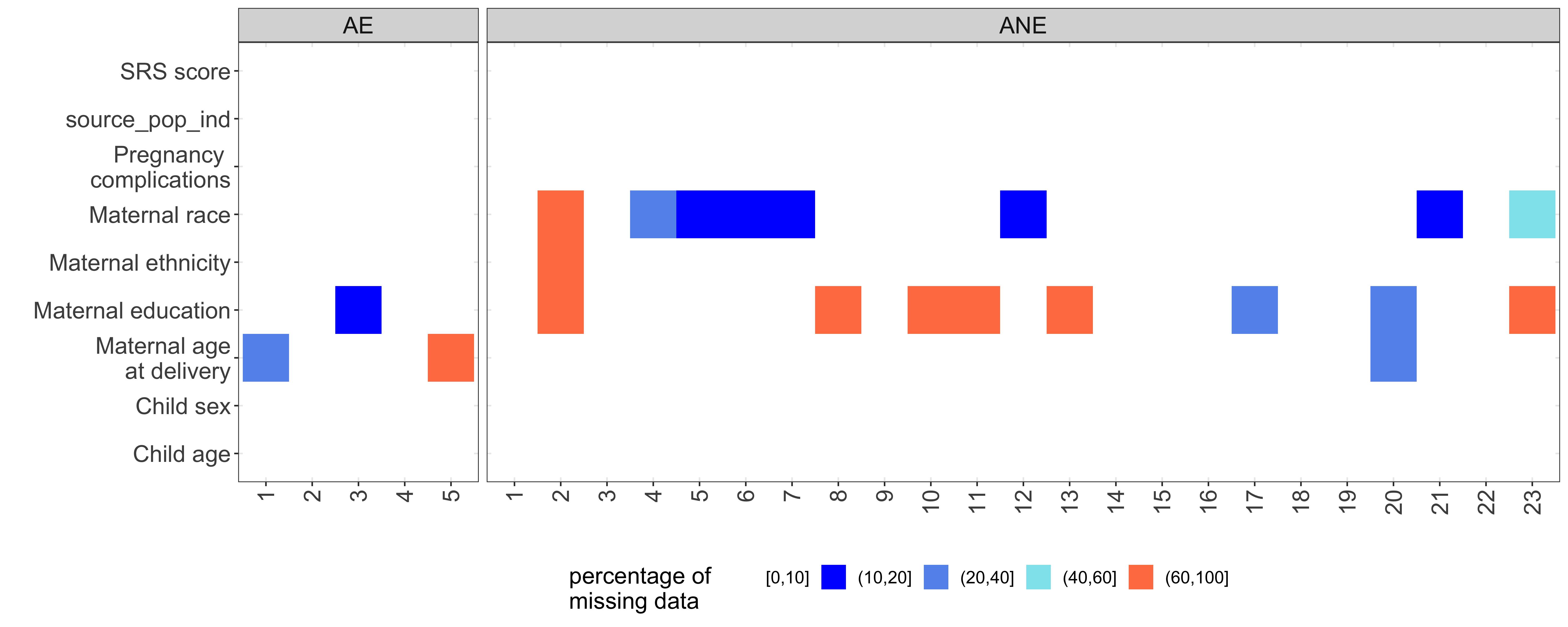
Figure 3: Missing data pattern for the cardiometabolic pregnancy complications to offspring autism spectrum disorder study. The color scale represents the proportion of missing covariates (y-axis) for each cohort (x-axis). Cohorts are grouped by corresponding study design: (1) autism enriched (AE) - cohorts with higher proportions of children with autism disorder; (2) autism not enriched (ANE) - cohorts with a regular proportion of children with autism disorder.

Linear models (R function lm) were used to fit the models. The proposed relate approach identified seven groups of similar cohorts, two of which was comprised of only a single cohort: (1) Columbia Center for Children’s Environmental Health (CCCEH); and (2) the study effects of potentially modifiable exposures during pregnancy and after birth (Project Viva). It is not surprising that the CCCEH cohort was not grouped with other cohorts in the study: this cohort was unique comprised of women identified as Dominican or African American and lived in Manhattan or South Bronx, NY. Both studies had cohort-level missing data and were removed from the analysis. For the imputation from cohorts with similar study design, we imputed the data within five autism-enriched cohorts and within the remaining cohorts separately.

The estimated regression coefficients and corresponding significance values are presented in Table 4. The estimated regression coefficients and corresponding significance levels are similar for the pooled cohorts and similar study design imputation methods, and are different from the proposed relate approach for the covariates: college education and race (American Indian and more than one race). These results suggest that similarity in study design does not necessarily imply similarity in covariate distribution for these cohorts. Therefore, imputing data from either pooled cohorts or large clusters of similar study design may often lead to violation of an assumption of similarity in data distributions used for imputation. While the underlying truth is unknown, we argue that using smaller clusters of cohorts with potentially similar distributions is a more reasonable approach to avoid changing the associations between exposures and outcomes.

Table 4: Comparison of the estimated regression coefficients for prediction of SRS scores using (1) total: imputation from the cohorts with available data on a missing covariate; (2) similar design: imputation from the cohorts with similar study design; and (3) RF asymptotic: imputation from the clusters of similar cohorts identified by the proposed random forest method.

	Total		Similar design		RF asymptotic
	Estimate	P-value	Estimate	P-value	Estimate	P-value
Intercept	40.361	$<0.001$	42.252	$<0.001$	40.474	$<0.001$
Child’s sex	-5.992	$<0.001$	-5.971	$<0.001$	-6.406	$<0.001$
Child age	0.723	$<0.001$	0.747	$<0.001$	0.848	$<0.001$
Maternal race
Black	6.621	$<0.001$	6.954	$<0.001$	4.579	$<0.001$
Asian	6.589	$<0.001$	7.006	$<0.001$	5.256	0.001
Native Hawaiian or other Pacific	0.544	0.926	2.899	0.681	1.359	0.852
American Indian or Alaska Native	7.427	0.005	6.884	0.017	7.718	0.852
More than one race	4.470	0.003	4.158	0.008	2.327	0.171
Other	0.628	0.781	1.240	0.620	-2.999	0.254
Hispanic	2.436	0.022	2.788	0.008	2.499	0.041
Maternal age at delivery	0.082	0.124	0.022	0.683	0.037	0.560
Maternal Education
below high school	-2.200	0.148	-2.015	0.195	0.709	0.654
some college	-4.975	$<0.001$	-5.131	$<0.001$	-1.463	0.326
Bachelors	-10.882	$<0.001$	-10.612	$<0.001$	-7.803	$<0.001$
Masters and above	-11.939	$<0.001$	-12.033	$<0.001$	-9.743	$<0.001$
Pregnancy complication	4.467	$<0.001$	4.428	$<0.001$	3.665	$<0.001$

5 Discussion

We introduced a procedure for extending the methods for missing data interpolation to the case of heterogeneous multi-cohort data where assumptions of the joint distribution of the variables pertinent to the analyses may be violated. The proposed approach groups ICS together, and then recursively assesses the similarity in distributions between the pairs of grouped data. We implement our procedure in R software package relate and illustrate applications on two ECHO studies. Our extensive simulations suggest that the proposed methodology correctly groups similar cohorts when the number of cohort groups with similar distributions is small.

The methodological novelty of our work is in the development of a combined approach for identifying groups with similar distributions using the random forest algorithm to define cohorts similarity based on the ability of covariates to predict cohort membership. The hierarchical clustering applied to the random forest distance further identifies the groups of cohorts with potentially similar distributions, which is formally tested using the BG test. This approach substantially reduces computational time needed for pairwise group comparisons of distributional similarity and makes the methodology feasible to implement in pooled cohort studies with over 1,000 observations per cohort. Crucially, this is the first study that attempts to systematically interpolate large heterogeneous data with cohort-level missing covariate data. Our results show that the cohorts grouped using the proposed methodology reflect the similarities in study design (i.e., grouping of all NICU cohorts together).

Our method has several limitations. First, we assume that the data is missing at random (MAR); that is covariates were not collected because of resources and none of participating cohorts purposefully decided not to collect missing covariates. Second, while we used random forest approach followed by hierarchical clustering algorithm, our method’s performance may change with alternative superlearning (i.e., a diverse library of data-adaptive algorithms to create the best weighted combination of candidate algorithms to further improve performance) algorithms (Naimi and Balzer, 2018) and clustering approaches; selection of an optimal learning approach is a topic for future research. Third, as illustrated in two applied ECHO data examples, relate does not necessarily combine all cohorts together which results in singleton cohorts with missing data that have to be excluded from the analysis. On the other hand, this may also be interpreted as an advantage of the proposed method that identifies dissimilar cohorts that should not be grouped with other data for interpolation purposes. Forth, we assume that the sample size is large enough to apply asymptotic distribution of the BG test statistic. Fifth, based on our simulations, we suggest not to impute while running BG test and not no apply relate in small studies with 3-4 cohorts. However, obtaining theoretical foundations to support these findings is a topic for future research. Finally, we suggest that the relate cohort groupings are evaluated by the by the subject expert prior to imputation and final analysis.

6 Software

Software in the form of R code, together with a sample input data set and complete documentation is available on github (https://yqzhong7.github.io/relate/).

7 Supplementary Material

Supplementary material is available online at http://biostatistics.oxfordjournals.org.

References

- Azur and others (2011) Azur, Melissa J, Stuart, Elizabeth A, Frangakis, Constantine and Leaf, Philip J. (2011). Multiple imputation by chained equations: what is it and how does it work? International journal of methods in psychiatric research 20(1), 40–49.
- Biswas and Ghosh (2014) Biswas, Munmun and Ghosh, Anil K. (2014). A nonparametric two-sample test applicable to high dimensional data. Journal of Multivariate Analysis 123, 160–171.
- Breiman (2003) Breiman, Leo. (2003). Manual on setting up, using, and understanding random forests v4. 0. Statistics Department University of California Berkeley, CA, USA, 1–33.
- Constantino and Gruber (2012) Constantino, John N and Gruber, Christian P. (2012). Social responsiveness scale: SRS-2. Western psychological services Torrance, CA.
- Cushing and others (2015) Cushing, Lara, Faust, John, August, Laura Meehan, Cendak, Rose, Wieland, Walker and Alexeeff, George. (2015). Racial/ethnic disparities in cumulative environmental health impacts in california: evidence from a statewide environmental justice screening tool (calenviroscreen 1.1). American journal of public health 105(11), 2341–2348.
- Donders and others (2006) Donders, A Rogier T, Van Der Heijden, Geert JMG, Stijnen, Theo and Moons, Karel GM. (2006). A gentle introduction to imputation of missing values. Journal of clinical epidemiology 59(10), 1087–1091.
- Gillman and Blaisdell (2018) Gillman, Matthew W and Blaisdell, Carol J. (2018). Environmental influences on child health outcomes, a research program of the nih. Current opinion in pediatrics 30(2), 260.
- Gordon (1999) Gordon, Allan David. (1999). Classification. CRC Press.
- Kundu and others (2019) Kundu, Prosenjit, Tang, Runlong and Chatterjee, Nilanjan. (2019). Generalized meta-analysis for multiple regression models across studies with disparate covariate information. Biometrika 106(3), 567–585.
- Legendre and Legendre (2012) Legendre, Pierre and Legendre, Louis. (2012). Numerical ecology. Elsevier.
- Lesko and others (2018) Lesko, Catherine R, Jacobson, Lisa P, Althoff, Keri N, Abraham, Alison G, Gange, Stephen J, Moore, Richard D, Modur, Sharada and Lau, Bryan. (2018). Collaborative, pooled and harmonized study designs for epidemiologic research: challenges and opportunities. International journal of epidemiology 47(2), 654–668.
- Little and Rubin (2019) Little, Roderick JA and Rubin, Donald B. (2019). Statistical analysis with missing data, Volume 793. John Wiley & Sons.
- Lyall and others (2022) Lyall, Kristen, Ning, Xuejuan, Aschner, Judy L, Avalos, Lyndsay A, Bennett, Deborah H, Bilder, Deborah A, Bush, Nicole R, Carroll, Kecia N, Chu, Su H, Croen, Lisa A and others. (2022). Cardiometabolic pregnancy complications in association with autism-related traits as measured by the social responsiveness scale in echo. American journal of epidemiology 191(8), 1407–1419.
- Mantero and Ishwaran (2021) Mantero, Alejandro and Ishwaran, Hemant. (2021). Unsupervised random forests. Statistical Analysis and Data Mining: The ASA Data Science Journal 14(2), 144–167.
- Martenies and others (2022) Martenies, Sheena E, Zhang, Mingyu, Corrigan, Anne E, Kvit, Anton, Shields, Timothy, Wheaton, William, Bastain, Theresa M, Breton, Carrie V, Dabelea, Dana, Habre, Rima and others. (2022). Associations between combined exposure to environmental hazards and social stressors at the neighborhood level and individual perinatal outcomes in the echo-wide cohort. Health & Place 76, 102858.
- Naimi and Balzer (2018) Naimi, Ashley I and Balzer, Laura B. (2018). Stacked generalization: an introduction to super learning. European journal of epidemiology 33(5), 459–464.
- Rubin (1976) Rubin, Donald B. (1976). Inference and missing data. Biometrika 63(3), 581–592.
- Stuart and others (2009) Stuart, Elizabeth A, Azur, Melissa, Frangakis, Constantine and Leaf, Philip. (2009). Multiple imputation with large data sets: a case study of the children’s mental health initiative. American journal of epidemiology 169(9), 1133–1139.