Present address: ]Department of Chemical Engineering, University College London, London WC1E 7JE, United Kingdom

Resolving the microscopic hydrodynamics at the moving contact line

Abstract

The molecular structure of moving contact lines (MCLs) and the emergence of a corresponding macroscopic dissipation have made the MCL a paradigm of fluid dynamics. Through novel averaging techniques that remove capillary waves smearing we achieve an unprecedented resolution in molecular dynamics (MD) simulations and find that they match with the continuum description obtained by finite element method (FEM) down to molecular scales. This allows us to distinguish dissipation at the liquid-solid interface (Navier-slip) and at the contact line, the latter being negligible for the rather smooth substrate considered.

Controlling the properties of MCLs is key to many modern technological applications including printable photovoltaics Berry et al. (2017), ink-jet printing Singh et al. (2010), liquid coating and paint drying processes Deegan et al. (2000). However, modeling the MCL is complicated because continuum descriptions often fail to describe the fluids microstructure in its proximity. A naive approach based on the no-slip boundary condition encounters a non-integrable stress singularity, raising what is known as the Huh-Scriven paradox Huh and Scriven (1971). Several mechanisms have been proposed to remove the singularity at the MCL present in dynamic wetting Neto et al. (2005); Bonn et al. (2009); Snoeijer and Andreotti (2013); Lu et al. (2016). Among these mechanisms are, for example, the Cox-Voinov law Voinov (1976); Cox (1986), the molecular-kinetic theory Blake and Haynes (1969); Blake and De Coninck (2002) and the interface formation theory Shikhmurzaev (1997, 1993). Notably, all these approaches rely on the introduction of a microscopic length scale below which the classical hydrodynamics of a homogeneous, incompressible, Newtonian fluid fails. To extend the applicability of hydrodynamics, additional dissipation mechanisms have been suggested, including Navier-slip Lauga et al. (2007) and MCL dissipation De Ruijter et al. (1999); de Gennes (1985). In addition, this picture is further complicated by the number of physical mechanisms that can contribute to the dissipation at the liquid/solid interface Müser et al. (2003); Krim (2012), including phonons Cieplak et al. (1994); Tomassone et al. (1997), electronic excitations  Tomassone and Widom (1997), and charge build-up Burgo et al. (2013).

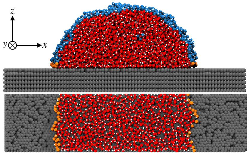
Figure 1: MD snapshot of a cylindrical droplet with 7,332 water molecules in a box $L_{x}\times L_{y}\times L_{z}=198.9\,\textrm{\AA}\times 46.8\,\textrm{\AA}\times 170\,\textrm{\AA}$ and external acceleration of $5\times 10^{-3}\textrm{\AA}/$ps² along the $x$-direction. Red: oxygen atoms; Blue: oxygen atoms at the liquid/vapor interface; Orange: oxygen atoms at the MCL; Gray: carbon atoms of the substrate. Top: side view; Bottom: top view of the first water layer

Accordingly, a detailed picture is needed to understand these phenomena at the molecular scale in the MCL region. MD simulations can deliver a microscopically detailed picture of the MCL Qian et al. (2003) and have been successful on many fronts, for example, in evidencing the breakdown of local hydrodynamics Thompson and Robbins (1989), providing support for the molecular-kinetic theory both with simple Bertrand et al. (2009) and hydrogen-bonding substrates Lācis et al. (2020) or investigating the time scale for the liquid/solid tension relaxation Lukyanov and Likhtman (2013). In previous MD studies, the fluid flow at the contact line was affected by evaporation Freund (2003) and significant contact line dissipation emerged from strong hydrogen bonding at the liquid-solid interface Johansson and Hess (2018), neither of which plays a role in our work.

Despite the potential for providing information at the molecular scale, the presence of thermal capillary waves Rowlinson and Widom (2002) is setting a limit to the resolution one can achieve close to the liquid/vapor interface. Capillary wave theory Buff et al. (1965) predicts that spontaneous surface excitations broaden the width of fluid interfaces with a logarithmic divergence that depends on the simulation cell size. For small molecular liquids and typical simulation cells, these fluctuations are larger than the molecular size Rowlinson and Widom (2002); Chacón and Tarazona (2003) at room temperature. Several computational strategies have been devised to recover the intrinsic structure of fluid interfaces Werner et al. (1997, 1999); Chacón and Tarazona (2003); Jorge and Cordeiro (2007); Pártay et al. (2008); Willard and Chandler (2010); Sega et al. (2013a). In some of these, including the approach reported here, one first identifies molecules at the phase interface as shown in Fig. 1, then uses them to define a local coordinate system. In turn, one can use this coordinate system to compute the profiles of chosen observables as a function of the local distance from the interface. To obtain further insight into the dynamics of the molecules at the MCL, one has to cope with its fluctuations. In this case, however, two interfaces are involved (liquid/vapor and liquid/solid), and one-dimensional intrinsic profiles are not enough to describe the system. Here, we extend the approach of intrinsic profiles to the region around the three-phase contact line by introducing two-dimensional density maps that are functions of the position relative to the liquid/vapor and liquid/solid interfaces, respectively. This procedure allows us to resolve the structure and the flow close to the MCL at an unprecedented resolution.

We performed MD simulations of a cylindrical water droplet moving on a rigid substrate under the influence of a constant acceleration parallel to the solid surface. Water is modeled using the SPC/E potentialBerendsen et al. (1987) and the substrate as a rigid, graphite-like structure with defects Sega et al. (2013b), obtained by removing 35% of randomly selected surface atoms. The presence of defects serves rather well the purpose of providing a friction coefficient thanks to the lateral modulation of the water-surface interaction potential. All molecular dynamics simulations are performed with an in-house modified version of the GROMACS simulation package, release 2019.4Abraham et al. (2015), that uses a Nosé-Hoover Nosé (1984); Hoover (1985) thermostat coupled only to the direction orthogonal to both the surface normal and the external forceThompson and Robbins (1989), keeping in mind that this introduces a bias in the surface energies Sega and Jedlovszky (2018). Further details are reported in the Supplemental Materialsup . Input files and GROMACS source code patch are provided in a dataset available on ZenodoGiri et al. (2022).

The first step in computing intrinsic maps of the droplet’s hydrodynamic fields is identifying the surface molecules at the liquid/vapor interface, cf. Fig. 1. Here, as detailed in the Supplemental Materialsup , we use the GITIM algorithm Sega et al. (2013a) as implemented in the Pytim packageSega et al. (2018).

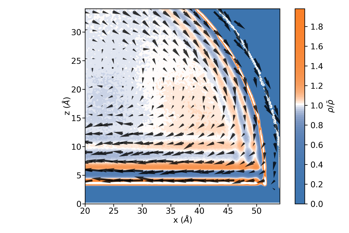
Figure 2: Intrinsic map of the density (color) and velocity field in the co-moving reference frame (arrows). The molecules belonging to the liquid/vapor interface have zero inherent distance $\xi_{V}$ and are represented here using the result of an elliptic fit through their average position (small open circles). The density field has resolution $0.22\,\textrm{\AA}\times{}0.2\,\textrm{\AA}$ and is normalized with respect to the bulk density. The velocity field has resolution $1.7\,\textrm{\AA}\times{}1.6\,\textrm{\AA}$ and is scaled such that an arrow of length 1 Å on the plot corresponds to a velocity of 0.01 Å/ps.

The surface molecules are used to provide the location of the (continuum) liquid/vapor $\bm{\zeta}_{V}(\bm{r})$ and liquid/solid $\bm{\zeta}_{S}(\bm{r})$ interfaces by using a linear interpolation between neighboring triplets of surface molecules. We compute the intrinsic map of a generic local observable $A$ as $A(\bm{\xi})=\left\langle\sum_{i}A_{i}\prod_{\alpha}\delta\left(\xi_{\alpha}-\min\left|\bm{r}_{i}-\bm{\zeta}_{\alpha}\right|\right)\right\rangle/{N(\bm{\xi})}.$ Here, $\alpha=\{V,S\}$ labels the liquid/vapor and liquid/solid interfaces and $\bm{\xi}=(\xi_{V},\xi_{S})$ are the distances of a point in space from the two surfaces. The angular brackets indicate a statistical average over time, and the index $i$ labels particles. The normalization factor $N(\bm{\xi})$ is calculated from the intrinsic density map of uniformly distributed random points within the liquid phase. The two-dimensional intrinsic map $A(\bm{\xi})$ is best interpreted if remapped back from the generalized coordinates $(\xi_{V},\xi_{S})$ to the Cartesian ones using the average location of the interfaces as the origin of the local frame. This approach provides precise information close to the liquid/vapor interface but loses accuracy far away from the interface. However, this region is not of concern for the current investigation, which focuses on the neighborhood of the MCL.

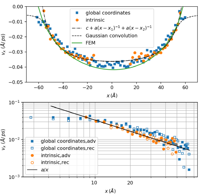
Figure 3: Top panel: horizontal velocity profiles (squares: global coordinate system, circles: intrinsic profiles) sampled along $x$ at $z=3\pm 3\,\textrm{\AA}$. The dot-dashed curve is a fit to a power law $c+a(x-x_{1})^{-1}+a(x_{2}-x)^{-1}$. The dashed line is the convolution of the best-fit power law with a Gaussian as described in the text ($a=-0.435\,\textrm{\AA}{}^{2}/\mathrm{ps}$, $c=-0.0495\,\textrm{\AA}/\mathrm{ps}$, $x_{1}=66.42\,\textrm{\AA}$, $x_{2}=-66.33\,\textrm{\AA}$). The green curve is the FEM solution evaluated at the interface $z=0$. Bottom panel: double logarithmic scale, same data as in the top panel but symmetrized along the vertical axis and shifted so that the fitting constants $c$ and $x_{1}$ are zero ($a=0.335\,\textrm{\AA}{}^{2}/\mathrm{ps}$).

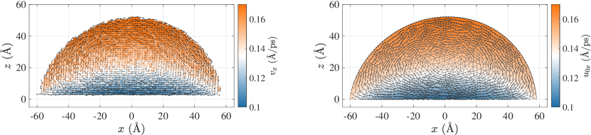
Figure 4: (Left: averaged MD velocity profile $\bm{v}=(v_{x},v_{z})$ (shown for $\rho>0.66\bar{\rho}$); Right: optimal Stokes velocity profile $\bm{u}_{0}=(u_{0x},u_{0z})$ for $\beta=1.38$ (slip-length $b=40\textrm{\AA})$ and $\delta=0$, $\mathrm{Bo}=0.2414$ and $\vartheta_{\mathrm{e}}=97.2^{\circ}$ in a comoving frame (vectors) and absolute horizontal velocity (shading).

The intrinsic density field reported in Fig. 2 reveals the oscillations associated to molecular layering at both the liquid/solid and liquid/vapor interfaces. In particular, a pronounced gap region due to hard-core repulsion appears next to both interfaces. As shown in Fig. 2, the resolution of the velocity field matches the molecular scale, with bins of size $1.7\,\textrm{\AA}\times 1.6\,\textrm{\AA}$, while the density bins are of size $0.22\,\textrm{\AA}\times 0.2\,\textrm{\AA}$. We do not observe any trace of an influence of positional correlations on the velocity field, which is a much smoother function of the position than the density. It is often remarked that continuum hydrodynamics breaks down in simple liquids below scales of few molecular diameters Chung and Yip (1969); Ailawadi et al. (1971). However, this is true for processes like sound propagation that, at that scale, happen during extremely short times on the order of a picosecond. In contrast, we compute the stationary fields of the hydrodynamic quantities by averaging over time intervals so large that no memory effect can survive.

The density map is in fact a correlation function and the oscillations can be interpreted as in a pair correlation function. The local density, computed as the (reciprocal) average volume available for each atom, is constant over the whole liquid phase and the droplet is incompressible (see plot of $\nabla\cdot\mathbf{v}$ in Fig. A8 of the Supplemental Materialsup ) down to and below the molecular scale. Therefore, the stationary velocity field that we compute from MD data can be modeled as that of a homogeneous incompressible fluid in the FEM simulations.

In Fig. 3 we report the horizontal velocity profile for molecules in the slab $z<6\textrm{\AA}$, computed in the droplet co-moving frame using both the global and intrinsic coordinate systems. The velocity sampled in the global coordinate system extends further than the intrinsic one because of the fluctuations. Both profiles coincide in the region $|x|<50\textrm{\AA}$, showing a steep increase when departing from the droplet center. However, close to the MCL, the velocity profile computed in the global coordinate system flattens out. In contrast, the intrinsic one is compatible over its entire extension with a power-law slip profile. The profile in the global coordinate system can be very well described in the spirit of the capillary wave theory by using quantities $\widetilde{A}(x)=\int_{0}^{L_{x}}G(x-x^{\prime})A(x^{\prime}){\rm d}x^{\prime}$ convoluted with the Gaussian distribution $G(x)\sim{}\exp[-x^{2}/(2\sigma^{2})]$ of the interface fluctuations, so that $v_{x}=\widetilde{p}_{x}/\widetilde{\rho}$. Here, $A(x)$ is the profile of observable $A$ averaged over the whole range in $y$ direction and over the first molecular layer in $z$ direction.

In the top panel of Fig. 3 we report as a dashed-line the velocity profile obtained by applying this convolution procedure to the best fit intrinsic velocity profile $v_{x}\sim(x-x_{1})^{-1}+(x_{2}-x)^{-1}$ and a step-like density profile, using the interfacial layer width $\sigma=2.5\textrm{\AA}$. The resulting profile reproduces very well the flattening in the region close to the MCL. These features are more evident in the double logarithmic scale, reported in the right panel of Fig. 3, where we have symmetrized the profile around its minimum and shifted it vertically and horizontally by the fitting constants $x_{1}$ and $c$. Our results show that after removing the capillary fluctuations via the intrinsic map method, the power-law behavior extends over the entire range down to the molecular length scale, and the previously reported departure from the power-lawQian et al. (2004) is due to the smearing introduced by capillary waves rather than a breakdown of hydrodynamics at short length scales.

The present computational approach allows us to discuss some of the proposed corrections to continuum models. We compare our MD simulation results with a full hydrodynamic continuum model for the MCL, where we solve a Stokes problem for an incompressible viscous Newtonian fluid (Re=0) featuring a free interface subject to capillary forces, which is driven by a constant acceleration $\bm{g}$. Dissipative processes are included by the combination of Navier-slip, i.e., $\beta u_{x}=\mu\partial_{z}u_{x}$, and dynamic contact line dissipation Ren and E (2007), i.e., $\nu_{x}\cdot u_{x}=\gamma/\delta(\cos\theta_{\mathrm{e}}-\cos\theta)$. The slip parameter $\beta$ enhances the inhomogeneity in the flow by increasing $\partial_{z}u_{x}$. In contrast, the contact line friction $\delta$ enhances the asymmetry of the droplet shape through advancing and receding contact angle, e.g., cf. Fig. A5 of the Supplemental Materialsup . Note that we use constant slip length and contact line dissipation, as space-dependent coefficients would yield an overdetermined improved fit but not lead to new physical insights. We discretize the system of partial differential equations using the isoparametric $\bm{P}_{2}-P_{1}$ Taylor-Hood finite elements combined with an ALE mesh motion strategy, for details cf. the Supplemental Materialsup and Refs. Peschka (2018); Montefuscolo et al. (2014).

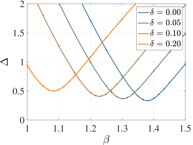
Figure 5: Rmsd $\Delta$ between FEM and MD flow fields for different dissipation parameters $\beta$ (Navier-slip) and $\delta$ (contact line) in the hydrodynamic Stokes model.

For a given acceleration $\bm{g}$ and droplet size $L$, we compare the velocity of traveling-wave solutions from the Stokes problem $\bm{u}(t,\bm{r})=\bm{u}_{0}(x-v_{0}t,z)$ with the corresponding velocity from the MD problem by computing the root mean square deviation (rmsd) $\Delta$, relative to the MD accuracy, with $\Delta{}^{2}=\int_{\Omega_{0}}\rho|\bm{u}_{0}-\bm{v}|^{2}/\delta\bm{v}^{2}{\,\rm d}x{\,\rm d}z\big{/}\int_{\Omega}\rho{\,\rm d}x{\,\rm d}z$, in the comoving frame $\Omega_{0}=\Omega-(v_{0},0)t$, where $\delta\bm{v}(x,z)$ is the space-dependent MD averaging error of $\bm{v}$. In Fig. 4 we show the excellent agreement of the horizontal components of MD and Stokes velocity for a droplet with optimized $\beta$ and $\delta$. Correspondingly, in Fig. 5 we show the rmsd $\Delta$ for different pairs of $\delta$ and $\beta$, where the optimal parameters suggest a vanishing or small contact line dissipation $0<\delta<0.05$ and $\beta=1.38$, corresponding to a slip-length $b=40\,\textrm{\AA}$. Because $\Delta$ is a relative measure of inaccuracy with respect to that of MD, we expect $\Delta\sim\mathscr{O}(1)$ for a good fit, similarly to a reduced $\chi^{2}$ test. For given $\delta$, the local minima in Fig. 5 suggest that also other parameters with larger $\delta$ and smaller $\beta$ are feasible. However, those parameters are not optimal for the prescribed bulk viscosity $\mu=0.7\,{\rm mPa\,s}$ but could possibly be improved by fitting the entire triple $(\mu,\beta,\delta)$, considering spatially inhomogeneous parameters or a compressibility of the fluid.

The water molecules are subjected to a friction force that, in steady-state conditions, balances $\bm{g}$ and is defined as the horizontal component of the force density $f_{\Gamma,x}(x,z)$ acting from the substrate on water molecules. Even though long-range corrections for dispersion forces are in place, the friction force becomes negligible at larger elevations $z\gtrapprox 10\,\textrm{\AA}$ and is acting almost exclusively on the first layer of water molecules at the substrate. Therefore, we can define a friction force per unit area as $F_{\Gamma}(x)=\int_{0}^{\infty}f_{\Gamma,x}(x,z){\rm d}z$. This force is the counterpart of the surface friction that in sharp interface models like the present FEM can be calculated from the stress $\bm{t}\cdot\bm{\sigma}\bm{\nu}\equiv-\mu_{\Gamma}\bm{t}\cdot\bm{u}$ at the solid-liquid interface, where $\bm{t}$ and $\bm{\nu}$ are the corresponding tangential and normal vectors. Fig. 6 shows the friction surface density $F_{\Gamma}$ obtained from the MD trajectories and compared to the FEM results. Far from the droplet edges, both force profiles are in excellent agreement. However, close to the advancing and receding MCL, the friction force behaves qualitatively differently. This mismatch contrasts the overall good match of the slip velocity profile Fig. 3. Therefore, even though the Navier-slip boundary condition is an excellent effective model in reproducing the slip velocity, the same is not true concerning the friction force near the MCL.

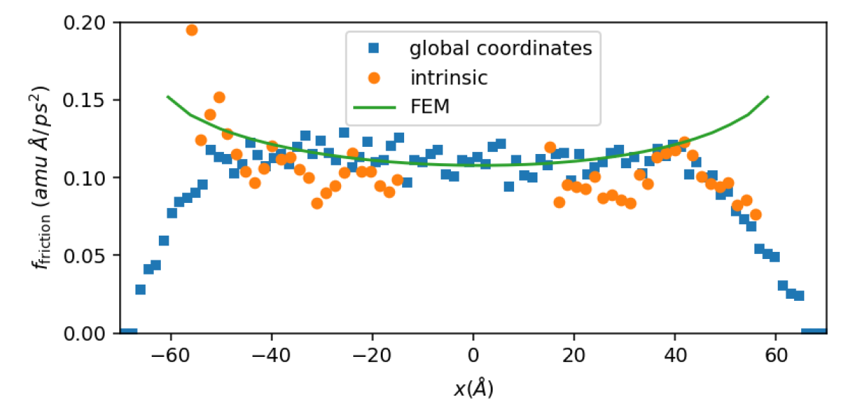
Figure 6: Profile of the friction surface density computed from the MD data in the global (squares) and intrinsic (circles) coordinate systems. The green curve is the FEM solution evaluated at the interface $z=0$.

This difference implies that the underlying dynamics is more complex than that encoded into the Navier-slip boundary condition. Remarkably, even in the present case, where the substrate is particularly smooth and the optimal FEM solution is compatible with zero contact line dissipation, we observe a significant deviation of the friction force from the one emerging from the Navier-slip boundary condition. Note that, upon integration of the force density in Fig. 6, this contribution is compatible with a contact line friction $\delta\lessapprox 0.05$. Larger defects or soft substrates will enhance this effect.

In this work, we compared microscopic MD simulations and hydrodynamic FEM simulations of sliding droplets with respect to their densities, flow and force fields at interfaces and MCLs. Using a novel averaging method, we showed that assumptions of continuum hydrodynamics are valid near the MCL. However, despite an effectively vanishing contact line friction, corrections to the force balance are clearly visible. In the future, larger droplets or elastic substrates with stronger roughness should be investigated to further enhance contact line friction and suppress density oscillations. Additionally, one should consider thermodynamics, compressibility, and evaporation of the liquid phase to better match continuum hydrodynamics with the microscopic interacting-particle system.

The datasets available on ZenodoGiri et al. (2022) provide MD input files, the GROMACS source code patch for the thermostat, averaged data from MD simulations (Cartesian mesh with mass density and velocity field) as well as FEM simulation solutions (triangular 2D droplet mesh with velocity field) in ASCII format, and MATLAB functions for the data import and plot generation. The MATLAB code is available at https://github.com/dpeschka/stokes-free-boundary/.

References

- Berry et al. (2017) Joseph J. Berry, Jao van de Lagemaat, Mowafak M. Al-Jassim, Sarah Kurtz, Yanfa Yan, and Kai Zhu, “Perovskite photovoltaics: The path to a printable terawatt-scale technology,” ACS Energy Lett. 2, 2540–2544 (2017).
- Singh et al. (2010) Madhusudan Singh, Hanna M. Haverinen, Parul Dhagat, and Ghassan E. Jabbour, “Inkjet Printing—Process and its applications,” Adv. Mater. 22, 673–685 (2010).
- Deegan et al. (2000) Robert D. Deegan, Olgica Bakajin, Todd F. Dupont, Greg Huber, Sidney R. Nagel, and Thomas A. Witten, “Contact line deposits in an evaporating drop,” Phys. Rev. E 62, 756 (2000).
- Huh and Scriven (1971) Chun Huh and L.E Scriven, “Hydrodynamic model of steady movement of a Solid/Liquid/Fluid contact line,” J. Colloid Interface Sci. 35, 85–101 (1971).
- Neto et al. (2005) Chiara Neto, Drew R Evans, Elmar Bonaccurso, Hans-Jürgen Butt, and Vincent S J Craig, “Boundary slip in Newtonian liquids: A review of experimental studies,” Rep. Prog. Phys. 68, 2859–2897 (2005).
- Bonn et al. (2009) Daniel Bonn, Jens Eggers, Joseph Indekeu, Jacques Meunier, and Etienne Rolley, “Wetting and spreading,” Rev. Mod. Phys. 81, 739–805 (2009).
- Snoeijer and Andreotti (2013) Jacco H. Snoeijer and Bruno Andreotti, “Moving Contact Lines: Scales, Regimes, and Dynamical Transitions,” Annu. Rev. Fluid Mech. 45, 269–292 (2013).
- Lu et al. (2016) Gui Lu, Xiao-Dong Wang, and Yuan-Yuan Duan, “A critical review of dynamic wetting by complex fluids: From Newtonian fluids to non-Newtonian fluids and nanofluids,” Adv. Colloid Interface Sci. 236, 43–62 (2016).
- Voinov (1976) O. V. Voinov, “Hydrodynamics of wetting,” Fluid Dyn. 11, 714–721 (1976).
- Cox (1986) R. G. Cox, “The dynamics of the spreading of liquids on a solid surface. Part 1. Viscous flow,” J. Fluid Mech. 168, 169–194 (1986).
- Blake and Haynes (1969) T.D Blake and J.M Haynes, “Kinetics of liquidliquid displacement,” J. Colloid Interface Sci. 30, 421–423 (1969).
- Blake and De Coninck (2002) T.D Blake and J De Coninck, “The influence of Solid–Liquid interactions on dynamic wetting,” Adv. Colloid Interface Sci. 96, 21–36 (2002).
- Shikhmurzaev (1997) Yulii D. Shikhmurzaev, “Moving contact lines in Liquid/Liquid/Solid systems,” J. Fluid Mech. 334, 211–249 (1997).
- Shikhmurzaev (1993) Yu D. Shikhmurzaev, “The moving contact line on a smooth solid surface,” Int. J. Multiph. Flow 19, 589–610 (1993).
- Lauga et al. (2007) Eric Lauga, Michael Brenner, and Howard Stone, “Microfluidics: The no-slip boundary condition,” in Springer Handbooks, Springer Handbooks (Springer, 2007) pp. 1219–1240.
- De Ruijter et al. (1999) Michel J. De Ruijter, Joël De Coninck, and G. Oshanin, “Droplet spreading: Partial wetting regime revisited,” Langmuir 15, 2209–2216 (1999).
- de Gennes (1985) P. G. de Gennes, “Wetting: Statics and dynamics,” Rev. Mod. Phys. 57, 827–863 (1985).
- Müser et al. (2003) Martin H. Müser, Michael Urbakh, and Mark O. Robbins, “Statistical Mechanics of Static and Low-Velocity Kinetic Friction,” in Advances in Chemical Physics, edited by I. Prigogine and Stuart A. Rice (John Wiley & Sons, Inc., Hoboken, NJ, USA, 2003) pp. 187–272.
- Krim (2012) Jacqueline Krim, “Friction and energy dissipation mechanisms in adsorbed molecules and molecularly thin films,” Adv. Phys. 61, 155–323 (2012).
- Cieplak et al. (1994) Marek Cieplak, Elizabeth D. Smith, and Mark O. Robbins, “Molecular Origins of Friction: The Force on Adsorbed Layers,” Science 265, 1209–1212 (1994).
- Tomassone et al. (1997) M. S. Tomassone, J. B. Sokoloff, A. Widom, and J. Krim, “Dominance of Phonon Friction for a Xenon Film on a Silver (111) Surface,” Phys. Rev. Lett. 79, 4798–4801 (1997).
- Tomassone and Widom (1997) M. S. Tomassone and A. Widom, “Electronic friction forces on molecules moving near metals,” Phys. Rev. B 56, 4938–4943 (1997).
- Burgo et al. (2013) Thiago A. L. Burgo, Cristiane A. Silva, Lia B. S. Balestrin, and Fernando Galembeck, “Friction coefficient dependence on electrostatic tribocharging,” Sci. Rep. 3, 2384 (2013).
- Qian et al. (2003) Tiezheng Qian, Xiao-Ping Wang, and Ping Sheng, “Molecular scale contact line hydrodynamics of immiscible flows,” Phys. Rev. E 68, 016306 (2003).
- Thompson and Robbins (1989) Peter A. Thompson and Mark O. Robbins, “Simulations of contact-line motion: Slip and the dynamic contact angle,” Phys. Rev. Lett. 63, 766–769 (1989).
- Bertrand et al. (2009) Emilie Bertrand, Terence D Blake, and Joël De Coninck, “Influence of Solid–Liquid interactions on dynamic wetting: A molecular dynamics study,” J. Phys.: Condens. Matter 21, 464124 (2009).
- Lācis et al. (2020) Uǧis Lācis, Petter Johansson, Tomas Fullana, Berk Hess, Gustav Amberg, Shervin Bagheri, and Stephané Zaleski, “Steady moving contact line of water over a no-slip substrate: Challenges in benchmarking phase-field and volume-of-fluid methods against molecular dynamics simulations,” Eur. Phys. J. Spec. Top. 229, 1897–1921 (2020).
- Lukyanov and Likhtman (2013) Alex V. Lukyanov and Alexei E. Likhtman, “Relaxation of Surface Tension in the Liquid–Solid Interfaces of Lennard-Jones Liquids,” Langmuir 29, 13996–14000 (2013).
- Freund (2003) Jonathan B. Freund, “The atomic detail of a wetting/de-wetting flow,” Phys. Fluids 15, L33–L36 (2003), https://doi.org/10.1063/1.1565112 .
- Johansson and Hess (2018) Petter Johansson and Berk Hess, “Molecular origin of contact line friction in dynamic wetting,” Phys. Rev. Fluids 3, 074201 (2018).
- Rowlinson and Widom (2002) John Shipley Rowlinson and Benjamin Widom, Molecular Theory of Capillarity (Dover Publications, Inc., Mineola, New York, 2002).
- Buff et al. (1965) F. P. Buff, R. A. Lovett, and F. H. Stillinger Jr, “Interfacial density profile for fluids in the critical region,” Phys. Rev. Lett. 15, 621 (1965).
- Chacón and Tarazona (2003) E. Chacón and P. Tarazona, “Intrinsic profiles beyond the capillary wave theory: A Monte Carlo study,” Phys. Rev. Lett. 91, 166103 (2003).
- Werner et al. (1997) Andreas Werner, Friederike Schmid, Marcus Müller, and Kurt Binder, “Anomalous size-dependence of interfacial profiles between coexisting phases of polymer mixtures in thin-film geometry: A Monte Carlo simulation,” J. Chem. Phys. 107, 8175–8188 (1997).
- Werner et al. (1999) A. Werner, F. Schmid, M. Müller, and K. Binder, ““Intrinsic” profiles and capillary waves at homopolymer interfaces: A Monte Carlo study,” Phys. Rev. E 59, 728–738 (1999).
- Jorge and Cordeiro (2007) Miguel Jorge and M. Natália DS Cordeiro, “Intrinsic structure and dynamics of the Water/Nitrobenzene interface,” J. Phys. Chem. C 111, 17612–17626 (2007).
- Pártay et al. (2008) Lívia B. Pártay, György Hantal, Pál Jedlovszky, Árpád Vincze, and George Horvai, “A new method for determining the interfacial molecules and characterizing the surface roughness in computer simulations. Application to the Liquid–Vapor interface of water,” J. Comput. Chem. 29, 945–956 (2008).
- Willard and Chandler (2010) Adam P. Willard and David Chandler, “Instantaneous Liquid Interfaces,” J. Phys. Chem. B 114, 1954–1958 (2010).
- Sega et al. (2013a) Marcello Sega, Sofia S. Kantorovich, Pál Jedlovszky, and Miguel Jorge, “The generalized identification of truly interfacial molecules (ITIM) algorithm for nonplanar interfaces,” J. Chem. Phys. 138, 044110 (2013a).
- Berendsen et al. (1987) H. J. C. Berendsen, J. R. Grigera, and T. P. Straatsma, “The missing term in effective pair potentials,” J. Phys. Chem. 91, 6269–6271 (1987).
- Sega et al. (2013b) Marcello Sega, Mauro Sbragaglia, Luca Biferale, and Sauro Succi, “Regularization of the slip length divergence in water nanoflows by inhomogeneities at the Angstrom scale,” Soft Matter 9, 8526–8531 (2013b).
- Abraham et al. (2015) Mark James Abraham, Teemu Murtola, Roland Schulz, Szilárd Páll, Jeremy C. Smith, Berk Hess, and Erik Lindahl, “GROMACS: High performance molecular simulations through multi-level parallelism from laptops to supercomputers,” SoftwareX 1–2, 19–25 (2015).
- Nosé (1984) Shūichi Nosé, “A molecular dynamics method for simulations in the canonical ensemble,” Mol. Phys. 52, 255–268 (1984).
- Hoover (1985) William G. Hoover, “Canonical dynamics: Equilibrium phase-space distributions,” Phys. Rev. A 31, 1695 (1985).
- Sega and Jedlovszky (2018) Marcello Sega and Pál Jedlovszky, “The impact of tensorial temperature on equilibrium thermodynamics,” Phys. Chem. Chem. Phys. 20, 16910–16912 (2018).
- (46) See Supplemental Material at [URL will be inserted by publisher] for or details on the MD and FEM simulations, effect of droplet size, slip length and contact line dissipation on the flow, density and velocity of the liquid/vapor surface layer, and compressibility map.
- Miyamoto and Kollman (1992) Shuichi Miyamoto and Peter A. Kollman, “Settle: An analytical version of the SHAKE and RATTLE algorithm for rigid water models,” J. Comput. Chem. 13, 952–962 (1992).
- Essmann et al. (1995) Ulrich Essmann, Lalith Perera, Max L. Berkowitz, Tom Darden, Hsing Lee, and Lee G. Pedersen, “A smooth particle mesh Ewald method,” J. Chem. Phys. 103, 8577–8593 (1995).
- Michaud-Agrawal et al. (2011) Naveen Michaud-Agrawal, Elizabeth J. Denning, Thomas B. Woolf, and Oliver Beckstein, “MDAnalysis: A toolkit for the analysis of molecular dynamics simulations,” J. Comput. Chem. 32, 2319–2327 (2011).
- Sega et al. (2018) Marcello Sega, György Hantal, Balázs Fábián, and Pál Jedlovszky, “Pytim: A python package for the interfacial analysis of molecular simulations,” J. Comput. Chem. 39, 2118–2125 (2018).
- Shvab and Sadus (2013) I. Shvab and Richard J. Sadus, “Intermolecular potentials and the accurate prediction of the thermodynamic properties of water,” J. Chem. Phys. 139, 194505 (2013).
- Sega and Dellago (2017) Marcello Sega and Christoph Dellago, “Long-Range Dispersion Effects on the Water/Vapor Interface Simulated Using the Most Common Models,” J. Phys. Chem. B 121, 3798–3803 (2017).
- Giri et al. (2022) Amal K. Giri, Paolo Malgaretti, Dirk Peschka, and Marcello Sega, Zenodo 706651 (2022), dataset for “Resolving the microscopic hydrodynamics at the moving contact line”.
- Chung and Yip (1969) Chang-Hyun Chung and Sidney Yip, “Generalized Hydrodynamics and Time Correlation Functions,” Phys. Rev. 182, 323–339 (1969).
- Ailawadi et al. (1971) Narinder K. Ailawadi, Aneesur Rahman, and Robert Zwanzig, “Generalized Hydrodynamics and Analysis of Current Correlation Functions,” Phys. Rev. A 4, 1616–1625 (1971).
- Qian et al. (2004) Tiezheng Qian, Xiao-Ping Wang, and Ping Sheng, “Power-Law Slip Profile of the Moving Contact Line in Two-Phase Immiscible Flows,” Phys. Rev. Lett. 93, 094501 (2004).
- Ren and E (2007) Weiqing Ren and Weinan E, “Boundary conditions for the moving contact line problem,” Phys. Fluids 19, 022101 (2007).
- Peschka (2018) D. Peschka, “Variational approach to dynamic contact angles for thin films,” Phys. Fluids 30, 082115 (2018).
- Montefuscolo et al. (2014) Felipe Montefuscolo, Fabricio S Sousa, and Gustavo C Buscaglia, “High-order ALE schemes for incompressible capillary flows,” J. Comput. Phys. 278 (2014), 10.1016/j.jcp.2014.08.030.