Converses to generalized Conway–Gordon type congruences
Abstract.
It is known that for every spatial complete graph on vertices, the summation of the second coefficients of the Conway polynomials over the Hamiltonian knots is congruent to modulo , where if , and if . In particular the case of is famous as the Conway–Gordon theorem. In this paper, conversely, we show that every integer is realized as the summation of the second coefficients of the Conway polynomials over the Hamiltonian knots in some spatial complete graph on vertices.
Key words and phrases:
Spatial graphs, Conway–Gordon theorem1991 Mathematics Subject Classification:
Primary 57M15; Secondary 57K101. Introduction
Throughout this paper we work in the piecewise linear category. An embedding of a finite graph into is called a spatial embedding of , and the image is called a spatial graph of . We say that two spatial graphs are ambient isotopic if there exists an orientation-preserving self-homeomorphism on which sends one to the other. We call a subgraph of homeomorphic to the circle a cycle of . We denote the set of all cycles of by . A cycle of is called a -cycle if it contains exactly vertices, and also called a Hamiltonian cycle if it contains all vertices of . We often denote an edge of connecting the vertices and by , and also denote a -cycle of by . We denote the set of all -cycles of by , and the set of all pairs of two disjoint cycles of consisting of a -cycle and a -cycle by . For a cycle (resp. a pair of disjoint cycles ) of and a spatial graph , (resp. ) is none other than a knot (resp. -component link) in . In particular for a Hamiltonian cycle of , we also call a Hamiltonian knot in .
Let be the complete graph on vertices, that is the graph consisting of vertices such that each pair of its distinct vertices and is connected by exactly one edge . Then, in 1983, the following congruence was given, which is well-known as the Conway–Gordon theorem.
Theorem 1-1.
(Conway–Gordon [2]) For any spatial embedding of , we have
| (1.1) |
where denotes the second coefficient of the Conway polynomial.
The modulo two reduction of for an oriented knot is also called the Arf invariant of . Theorem 1-1 says that a spatial graph always contains a nontrivial Hamiltonian knot with Arf invariant one. Even when , by applying Theorem 1-1, Blain et al. and Hirano showed that a spatial graph always contains a large number of such nontrivial Hamiltonian knots [1], [6].
On the other hand, in 2009, an integral lift of (1.1) was given by the author [10], and further extended to with by Morishita and the author in 2019 [8] (See Theorem 2-1). As a consequence, an extension of (1.1) to general complete graphs was also given as follows, that is a constraint on the set of all Hamiltonian knots in a spatial complete graph with arbitrary number of vertices.111The case of had previously been obtained by combining the results of Foisy [4] and Hirano [5].
Theorem 1-2.
Rephrasing Theorem 1-2, we learn that, if there exists a spatial embedding of such that then must be congruent to modulo . Our purpose in this paper is to show that the converse is also true. This means that the congruence (1.2) cannot be refined any further for every .
Theorem 1-3.
Let be an integer. For an integer , there exists a spatial embedding of such that if and only if .
For a spatial embedding of and a subset of , the modulo reduction of was denoted by in Shimabara [13] and the condition for it not to depend on was investigated.222Later, Lemma 2 in [13] was found to be incorrect and was modified in [4, Lemma 1]. Theorem 1-3 completely determines the maximum value of such that does not depend on , and also determines the possible values of as that time. We prove Theorem 1-3 in the next section. Our proof is constructive, namely for any integer , we construct a spatial embedding of satisfying .
Remark 1-4.
-
(1)
If we define , then we also will see that Theorem 1-3 is true for , namely every integer can be realized by .
- (2)
2. Proof of Theorem 1-3
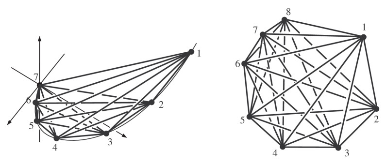
First of all, we prepare a kind of ‘canonical’ spatial embedding of . Let be a spatial embedding of constructed by taking all vertices of in order on the moment curve in and connecting every pair of two distinct vertices by a straight line segment, see Fig. 2.1 for . In [8], this is called a standard rectilinear spatial embedding of , and is also ambient isotopic to a canonical book presentation of introduced in [3]. We denote by . Let be the set of vertices of satisfying . Then induces a subgraph of isomorphic to . We denote this subgraph by . Then for any , the spatial subgraph of is ambient isotopic to .
To calculate the summation of over the Hamiltonian knots in a spatial complete graph, let us recall a generalized Conway–Gordon type theorem.
Theorem 2-1.
(Morishita–Nikkuni [8]) Let be an integer. For any spatial embedding of , we have
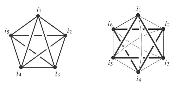
Therefore, to know the summation of over the Hamiltonian knots in a spatial complete graph, we only need to know the summation of over the ‘pentagon’ knots and the summation of over the ‘triangle-triangle’ links.
Example 2-2.
([8]) For an integer , let us calculate . As we said before, for any collection of vertices of , the spatial subgraph of is ambient isotopic to . Note that contains no nontrivial knots, and contains exactly one nonsplittable link which is a Hopf link, see Fig. 2.2. Then we have
Thus by Theorem 2-1, we have
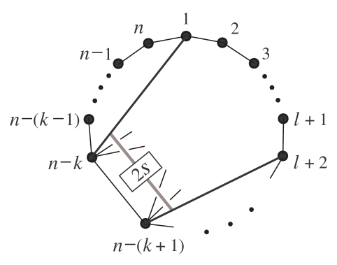
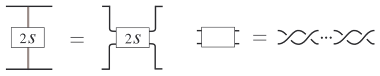
Let be an integer and non-negative integers satisfying . Then for a non-negative integer , we obtain a spatial graph from by twisting two spatial edges and times as illustrated in Fig. 2.3 and Fig. 2.4. Note that this twist is done close enough to the vertices and , and this twisted part represented by a gray segment with in the diagram as in Fig. 2.3 has no under crossings with any other edge.
Lemma 2-3.
where
Proof.
By Theorem 2-1, we have
In addition, in the same way as Example 2-2, we have
Here, we only need to consider containing two spatial edges and . First we consider containing and . There are six types of such graphs:
-
(1)
,
-
(2)
,
-
(3)
,
-
(4)
,
-
(5)
,
-
(6)
.
Then , , , , and are spatial graphs as illustrated in Fig. 2.5 (1), (2), (3), (4), (5) and (6), respectively.
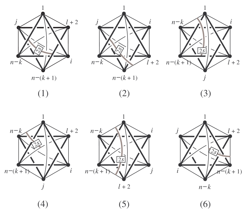
(1) We put and . Then we can see that , , and is a trivial link for any . Note that there are ways to choose a vertex , and there are ways to choose a vertex . Then we have
(2) We put , and . Then we can see that , , and is a trivial link for any . Note that there are ways to choose a vertex , and there are ways to choose a vertex . Then we have
| (2.5) |
(3) Note that there are ways to choose a vertex , and there are ways to choose a vertex . Then in the same way as (2), we have
(4) Note that there are ways to choose the vertices and . Then in the same way as (2), we have
| (2.7) |
(5) Note that there are ways to choose the vertices and . Then in the same way as (2), we have
| (2.8) |
(6) Note that there are ways to choose the vertices and . Then in the same way as (2), we have
| (2.9) |
Then by combining (2), (2.5), (2), (2.7), (2.8) and (2.9) with (2), we have
Next we consider containing and . There are three types of such graphs:
-
(1)
,
-
(2)
,
-
(3)
.
Then , and are spatial graphs as illustrated in Fig. 2.6 (1), (2) and (3), respectively.
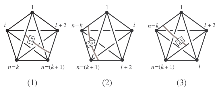
(1) We put and . Then we can see that is ambient isotopic to the -torus knot, is ambient isotopic to the -torus knot and is a trivial knot for any . We remark here that for the -torus knot . Also note that there are ways to choose a vertex . Then we have
(2) We put and . Then we can see that each of and is ambient isotopic to the -torus knot and is a trivial knot for any . Note that there are ways to choose a vertex . Then we have
| (2.12) |
As special cases of Lemma 2-3, we also have the following.
Lemma 2-4.
-
(1)
If is an odd integer, then
-
(2)
If is an even integer, then
On the other hand, we can always change the value of by as follows.
Lemma 2-5.
For any spatial embedding of , there exists a spatial embedding of such that
Proof.
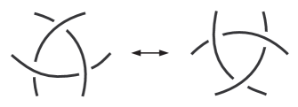
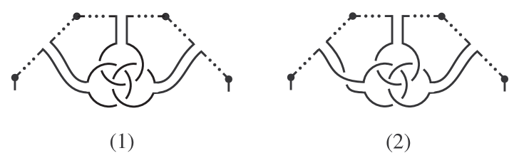
A delta move is a local move on a spatial graph as illustrated in Fig. 2.7 [9]. It is known that if two oriented knots and are transformed into each other by a single delta move, then [11]. In particular, a ‘band sum’ of Borromean rings as illustrated in Fig. 2.8 (1) (resp. (2)) causes to increase (resp. decrease) by exactly one. Since there are Hamiltonian cycles of containing a fixed path of length , we have the result. ∎
Proof of Theorem 1-3.
We show that for an integer , there exists a spatial embedding of such that . Since by Theorem 1-2, we have that for some integer . Here, for this integer , there uniquely exists an integer such that . Thus we have
Then by combining Lemma 2-4 with Lemma 2-5, there exists a spatial embedding of such that
This completes the proof. ∎
References
- [1] P. Blain, G. Bowlin, J. Foisy, J. Hendricks and J. LaCombe, Knotted Hamiltonian cycles in spatial embeddings of complete graphs, New York J. Math. 13 (2007), 11–16.
- [2] J. H. Conway and C. McA. Gordon, Knots and links in spatial graphs, J. Graph Theory 7 (1983), 445–453.
- [3] T. Endo and T. Otsuki, Notes on spatial representations of graphs, Hokkaido Math. J. 23 (1994), 383–398.
- [4] J. Foisy, Corrigendum to: “Knotted Hamiltonian cycles in spatial embeddings of complete graphs” by P. Blain, G. Bowlin, J. Foisy, J. Hendricks and J. LaCombe, New York J. Math. 14 (2008), 285–287.
- [5] Y. Hirano, Knotted Hamiltonian cycles in spatial embeddings of complete graphs, Docter Thesis, Niigata University, 2010.
- [6] Y. Hirano, Improved lower bound for the number of knotted Hamiltonian cycles in spatial embeddings of complete graphs, J. Knot Theory Ramifications 19 (2010), 705–708.
- [7] R. Karasev and A. Skopenkov, Some ‘converses’ to intrinsic linking theorems, Discrete Comput. Geom. 70 (2023), 921–930.
- [8] H. Morishita and R. Nikkuni, Generalizations of the Conway-Gordon theorems and intrinsic knotting on complete graphs, J. Math. Soc. Japan 71 (2019), 1223–1241.
- [9] H. Murakami and Y. Nakanishi, On a certain move generating link-homology, Math. Ann. 284 (1989), 75–89.
- [10] R. Nikkuni, A refinement of the Conway-Gordon theorems, Topology Appl. 156 (2009), 2782–2794.
- [11] M. Okada, Delta-unknotting operation and the second coefficient of the Conway polynomial, J. Math. Soc. Japan 42 (1990), 713–717.
- [12] H. Sachs, On spatial representations of finite graphs, Finite and infinite sets, Vol. I, II (Eger, 1981), 649–662, Colloq. Math. Soc. Janos Bolyai, 37, North-Holland, Amsterdam, 1984.
- [13] M. Shimabara, Knots in certain spatial graphs, Tokyo J. Math. 11 (1988), 405–413.