Diffusion models for missing value imputation in tabular data

Shuhan Zheng
The University of Tokyo
shuhanzheng@g.ecc.u-tokyo.ac.jp
&Nontawat Charoenphakdee
Preferred Networks
nontawat@preferred.jp
This work was done during his internship at Preferred Networks.

Abstract

Missing value imputation in machine learning is the task of estimating the missing values in the dataset accurately using available information. In this task, several deep generative modeling methods have been proposed and demonstrated their usefulness, e.g., generative adversarial imputation networks. Recently, diffusion models have gained popularity because of their effectiveness in the generative modeling task in images, texts, audio, etc. To our knowledge, less attention has been paid to the investigation of the effectiveness of diffusion models for missing value imputation in tabular data. Based on recent development of diffusion models for time-series data imputation, we propose a diffusion model approach called “Conditional Score-based Diffusion Models for Tabular data” (TabCSDI). To effectively handle categorical variables and numerical variables simultaneously, we investigate three techniques: one-hot encoding, analog bits encoding, and feature tokenization. Experimental results on benchmark datasets demonstrated the effectiveness of TabCSDI compared with well-known existing methods, and also emphasized the importance of the categorical embedding techniques.

^†^†footnotetext: Table Representation Learning Workshop at NeurIPS 2022

1 Introduction

In real-world applications, it is often the case that the dataset for training a prediction model contains missing values. This phenomenon can happen for many reasons, e.g., human error, privacy concerns, and the difficulty of data collection. For example, in census data, some people might not be comfortable to reveal their sensitive information such as employment information [1, 2]. In healthcare data, different patients may have taken different health examinations, which cause the dataset to have different available health features for each patient [3, 4]. Technically, the missing data problem can be divided into three categories: Missing completely at random (MCAR), Missing at random (MAR), Missing not at random (MNAR) (see Rubin [5] and Van Buuren [6] for more details).

According to Jarrett et al. [7], a missing value imputation approach can be divided into two categories. The first category is the iterative approach. It is based on the idea of estimating the conditional distribution of one feature using all other available features. In one iteration, we will train a conditional distribution estimator to predict the value of each feature. We will repeat the process for many iterations until the process is converged, i.e., the latest iteration does not change the prediction output significantly according to the pre-specified convergence criterion. This approach has been studied extensively [8, 9, 10, 7] and one of the most well-known methods is Multiple Imputation based on Chained Equations (MICE) [8]. The second category is a deep generative model approach. In this approach, we will train a generative model to generate values in missing parts based on observed values. Previous methods that can be categorized in this approach are Multiple Imputation using Denoising Autoencoders (MIDA) [11], Handling Incomplete Heterogeneous Data using Variational Autoencoders (HIVAE) [12], Missing Data Importance-weighted Autoencoder (MIWAE) [13], and Generative Adversarial Imputation Nets (GAIN) [14]. Recently, diffusion model is a generative model that has demonstrated its effectiveness over other generative models in various domains, e.g., computer vision [15, 16, 17], time-series data [18, 19], chemistry [20, 21], and natural language processing [22, 23]. However, to the best of our knowledge, a diffusion model has not been proposed yet for missing value imputation in tabular data.

The goal of this paper is to develop a diffusion model approach for missing value imputation based on the recent development of diffusion model approach for missing value imputation in time-series data called CSDI [18]. CSDI is originally designed for time-series data and it cannot support categorical variables, which are necessary for tabular data. To solve this problem, we propose a variant of CSDI called TabCSDI for tabular data by making it supports both the categorical and numerical features. Our experimental results show that TabCSDI can be successfully trained to achieve competitive performance to existing methods both in the iterative approach and generative approach. We can also observe that the choice of categorical embedding methods can affect performance.

2 Problem formulation

Let $\mathcal{X}=(\mathbb{R}\cup\{\varnothing\})^{d}$ be an input space, where $\mathbb{R}$ denotes a real number space and “ $\varnothing$ ” denotes a missing value. In missing value imputation, we are given $d$ -dimensional training dataset $\mathbf{X}_{\mathrm{tr}}=\{\mathbf{x}_{i}\}_{i=1}^{n}$ , where $n$ is the number of data. Without loss of generality, a feature $j\in\{1,\ldots,d\}$ of $\mathbf{x}_{i}$ is defined as $\mathbf{x}^{j}_{i}\in\mathcal{X}$ , where a feature can be missing, numerical variable, or categorical variable. This paper focuses on an inductive setting where the goal is to find an imputation function $f\colon\mathcal{X}\to\mathbb{R}^{d}$ that transforms the input that allows missing value $\mathcal{X}$ to the $d$ -dimension real values $\mathbb{R}^{d}$ . A desirable $f$ should be able to replace the missing values with reasonable values.

To evaluate the performance of $f$ , we are given test input data $\mathbf{X}_{\mathrm{te}}=\{\mathbf{x}_{i}\}_{i=1}^{n}$ and ground truths $\mathbf{Y}_{\mathrm{te}}=\{y^{j}_{i}\in\mathbb{R}\colon\mathbf{x}^{j}_{i}=\varnothing$ }. For $\mathbf{x}^{j}_{i}$ , we define $\widehat{\mathbf{x}}^{j}_{i}$ to be an imputed feature obtained from $f(\mathbf{x}_{i})$ for a feature $j$ . Let $M^{j}=\{i:\mathbf{x}^{j}_{i}=\varnothing\}$ be the set of missing value indices and $N^{j}_{\mathrm{miss}}=|M^{j}|$ be the number of missing values for a feature $j$ . To calculate the error of $f$ , we use the root mean squared error (RMSE) if $j$ is numerical and the error rate (Err) if $j$ is categorical:

\displaystyle\mathrm{RMSE}(j)=\sqrt{\frac{\sum_{i\in M^{j}}(\widehat{\mathbf{x}}^{j}_{i}-y^{j}_{i})^{2}}{N^{j}_{\mathrm{miss}}}},\quad\mathrm{Err}(j)=\frac{1}{N^{j}_{\mathrm{miss}}}\sum_{i\in M^{j}}\mathds{1}_{[\widehat{\mathbf{x}}^{j}_{i}\neq y^{j}_{i}]},

where $\mathds{1}_{[\cdot]}$ is an indicator function that returns $1$ if the condition holds and $0$ otherwise.

3 TabCSDI: Conditional Score-based Diffusion Models for Tabular data

In this section, we describe our proposed diffusion model method for missing value imputation in tabular data by describing CSDI [18] and how to modify it for handling tabular data.

3.1 Conditional Score-based Diffusion Model (CSDI)

Diffusion model contains two processes: the forward noising process where we iteratively inject the noise into the input data, and the reverse denoising process where we iteratively denoise the data. In the standard training process of diffusion model [15, 16], only the reverse process requires training while the forward process is always fixed. We omit the details of diffusion model for brevity (see Song and Ermon [15], Ho et al. [16] for more information).

Based on the idea of diffusion model, Tashiro et al. [18] recently proposed a diffusion model called CSDI for missing value imputation for time-series data. The key idea of CSDI can be explained as follows. Instead of reconstructing the whole input $\mathbf{x}$ by straightforwardly using the diffusion model, aka., unconditional diffusion model (see Appendix C of Tashiro et al. [18]), CSDI separates input $\mathbf{x}$ into two parts: the observed part (aka., conditional part) $\mathbf{x}^{co}$ and the unobserved part to predict (aka., target part) $\mathbf{x}^{ta}$ . The goal of the diffusion model is to model the following distribution:

p_{\theta}(\mathbf{x}^{ta}_{t-1}|\mathbf{x}^{ta}_{t},\mathbf{x}^{co}_{0})=\mathcal{N}(\mathbf{x}_{t-1}^{ta};\mathbf{\mu}_{\theta}(\mathbf{x}_{t}^{ta},t|\mathbf{x}^{co}_{0}),\sigma\mathbf{I}),

where $t\in\{1,\ldots,T\}$ denotes the iteration round of the process and $T$ is a hyperparameter. We need to model $\mathbf{\mu}_{\theta}$ that focuses only on predicting the values of the unobserved part. It is observed that the conditional diffusion model can achieve better performance than the unconditional one.

In our study, we followed the formulation of Tashiro et al. [18] as our objective function. For the architecture part, we slightly modified the architecture proposed in CSDI to appropriately handle tabular data. More specifically, we removed the temporal transformer layer of the original CSDI architecture since our data does not contain temporal information and use a simple residual connection of transformer encoder and multi-layered perceptron.

3.2 Handling categorical variables

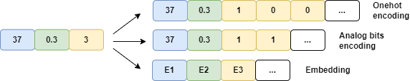
In the original CSDI, it is assumed that the input features contain only numerical variables, which is not the case for tabular data. In this section, we extend CSDI to support categorical variables by proposing three different techniques: (1) one-hot encoding, (2) analog bits encoding, and (3) feature tokenization. Figure 1 illustrates how each encoding works. The categorical variable is marked as yellow and we assume that there are three different categories for this feature. Without loss of generality, for one-hot encoding, the representation can be $[1,0,0]$ . For analog bits, we follow the encoding scheme proposed by Chen et al. [24]. In our example, the categorical variable will take two columns and represented in binary bits as $[1,1]$ . To make the data more distinguishable, we further convert $0$ to $-1$ in one-hot and analog bits encoding. For feature tokenizer [25], we transform both numerical and categorical variables together to embeddings. In our example, variables will have embedding vectors with the same length, i.e., $E_{1},E_{2},E_{3}\in\mathbb{R}^{e}$ . In sum, analog bits encoding takes less columns compared to one-hot encoding but will make the encoded vector complex. Feature tokenizer lets all variables have embeddings with the same length.

Then, we train the model with the processed input. After obtaining the raw output, different handling schemes require different recover procedures. For one-hot encoding, we treat the index of the largest element as the model inferred category. For analog bits encoding, we convert every output element to $1$ if the output element is larger than $0$ , otherwise we convert it to $-1$ . In the FT scheme, we need to recover both numerical and categorical variables back from the embeddings [25]. For numerical variables, we divide the diffusion model output by the corresponding embedding element-wise and use the average value as the final model output. For categorical variables, we calculate the Euclidean distance between TabCSDI outputs and every categorical embedding and set the category of closest embedding (i.e., $1$ -nearest neighbor) as the final model output.

Refer to caption — Figure 1: Example of handling categorical variables in one-hot encoding, analog bits encoding, and embeddings. The categorical variable is marked as the yellow block. Two numerical variables are marked as blue and green blocks.

4 Experimental results

In this section, we report experiments on pure numerical datasets and mixed variable datasets to show the effectiveness of TabCSDI.

Datasets: We used seven datasets. Census Income Data Set (Census), Wine Quality (Wine), Concrete Compressive Strength (Concrete), Libras Movement (Libras) and Breast Cancer Wisconsin (Breast) were obtained from UCI Machine Learning Repository [26]. COVID-19^†^†https://www.kaggle.com/datasets/tanmoyx/covid19-patient-precondition-dataset and Diabetes^†^†https://www.kaggle.com/datasets/alexteboul/diabetes-health-indicators-dataset were obtained from Kaggle. Dataset information is detailed in Appendix A. Note that Diabetes and COVID-19 datasets only have binary category variables and we preprocessed the numerical variables for all datasets by min-max normalization.

Comparison methods: In our experiments, we compare our proposed method with a simple baseline that uses training data’s mean values for numerical variables and mode values for categorical variables (Mean / Mode). We used MICE method with linear regression and logistic regression (MICE (linear)) and MICE method based on random forest (MissForest). We also used GAIN as a representative method for a deep generative model approach. The code implementation for MICE (linear), MissForest, and GAIN was provided by the Hyperimpute framework [7]^†^†https://github.com/vanderschaarlab/hyperimpute. For TabCSDI, we built our code based on CSDI [18]^†^†https://github.com/ermongroup/CSDI. Hyperparameter information is detailed in Appendix B.

Results: First, we show our results on three mixed variable datasets (Diabetes, Census and COVID-19). The following Table 1 shows the comparison between different imputation methods and categorical variable handling schemes. Our proposed methods (TabCSDI) reached the lowest RMSE in Diabetes and Census datasets. MissForest reached the lowest error rate in the Diabetes and Census datasets. The RMSE difference between three categorical handling methods was not evident. However, TabCSDI with FT obtained the lowest error rate in the Census dataset compared to other two categorical handling methods, where the analog bits approach is superior to one-hot. Second, we show our results on four pure numerical datasets in Table 2. It can be observed that our proposed TabCSDI has best performance against other comparison methods for three out of four datasets.

Table 1: RMSE and error rate performance for comparison methods on three mixed variable datasets. Note that one-hot and analog bits are equivalent for a dataset without multi-categorical variables.

	Diabetes		COVID-19		Census
	RMSE	Error rate	RMSE	Error rate	RMSE	Error rate
Mean / Mode	0.222 (0.003)	0.260 (0.004)	0.138 (0.002)	0.144 (0.002)	0.120 (0.003)	0.424 (0.003)
MICE (linear)	0.263 (0.002)	0.270 (0.004)	0.125 (0.003)	0.300 (0.038)	0.101 (0.002)	0.530 (0.011)
MissForest	0.216 (0.003)	0.214 (0.001)	0.120 (0.002)	0.131 (0.002)	0.112 (0.004)	0.300 (0.014)
GAIN	0.202 (0.003)	0.282 (0.005)	0.127 (0.002)	0.217 (0.011)	0.123 (0.057)	0.412 (0.012)
TabCSDI/ one-hot	0.197 (0.001)	0.222 (0.005)	0.122 (0.003)	0.111 (0.012)	0.099 (0.004)	0.400 (0.033)
TabCSDI/ analog bits	0.197 (0.001)	0.222 (0.005)	0.122 (0.003)	0.111 (0.012)	0.103 (0.004)	0.376 (0.013)
TabCSDI/ FT	0.206 (0.002)	0.224 (0.004)	0.123 (0.002)	0.107 (0.002)	0.098 (0.003)	0.345 (0.002)

Table 2: RMSE performance of comparison methods on four pure numerical datasets.

Methods	Wine	Concrete	Libras	Breast
Mean	0.076 (0.003)	0.217 (0.007)	0.099 (0.001)	0.263 (0.009)
MICE (linear)	0.065 (0.003)	0.153 (0.006)	0.034 (0.001)	0.154 (0.011)
MissForest	0.060 (0.002)	0.173 (0.005)	0.024 (0.001)	0.163 (0.014)
GAIN	0.072 (0.004)	0.203 (0.007)	0.089 (0.006)	0.165 (0.006)
TabCSDI	0.065 (0.004)	0.131 (0.008)	0.011 (0.001)	0.153 (0.003)

Discussions: Based on the results, TabCSDI is observed to be effective in imputing numerical variables, where it obtained the best RMSE performance for 5 out of 7 datasets. Different from previous generative models, the diffusion model performs decoding through a reverse process. TabCSDI can benefit from this iterative approximation reverse process, which allows the neural network to gradually figure out the target value. Moreover, our results suggest the effectiveness of FT in handling categorical variables. The superiority of FT is evident in the Census dataset (the only multi-category mixed data types dataset). One possible reason is that FT treats all variables equally. That is, all numerical variables will have embedding vectors with the same length. This strategy avoids the problem of column imbalance. Column imbalance can happen in one-hot and analog bits encoding, where the more categories the category variable contain, the more columns it will take.

5 Conclusions and future work

We have proposed a diffusion model-based method for missing value imputation called TabCSDI. We demonstrated that TabCSDI can obtain competitive performance with other well-known imputation methods. Particularly, TabCSDI works well for numerical variables imputation. We also explored different schemes for handling categorical variables and found that FT embedding gives evident better performance compared to one-hot encoding and analog bits in the Census dataset. Future work for TabCSDI that can be considered are (1) investigation of the inference time, (2) model architecture improvement, and (3) theoretical analysis of the loss function.

Acknowledgements

The authors would like to thank Shin-ichi Maeda, Kohei Hayashi, and Kenta Oono for helpful discussions during the PFN summer internship program 2022.

References

Lillard et al. [1986] Lee Lillard, James P Smith, and Finis Welch. What do we really know about wages? the importance of nonreporting and census imputation. Journal of Political Economy, 94(3, Part 1):489–506, 1986.
Eckert et al. [2020] Fabian Eckert, Teresa C Fort, Peter K Schott, and Natalie J Yang. Imputing missing values in the us census bureau’s county business patterns. Technical report, National Bureau of Economic Research, 2020.
Wells et al. [2013] Brian J Wells, Kevin M Chagin, Amy S Nowacki, and Michael W Kattan. Strategies for handling missing data in electronic health record derived data. Egems, 1(3), 2013.
Hegde et al. [2019] Harshad Hegde, Neel Shimpi, Aloksagar Panny, Ingrid Glurich, Pamela Christie, and Amit Acharya. Mice vs ppca: Missing data imputation in healthcare. Informatics in Medicine Unlocked, 17:100275, 2019.
Rubin [1976] Donald B Rubin. Inference and missing data. Biometrika, 63(3):581–592, 1976.
Van Buuren [2018] Stef Van Buuren. Flexible imputation of missing data. CRC press, 2018.
Jarrett et al. [2022] Daniel Jarrett, Bogdan C Cebere, Tennison Liu, Alicia Curth, and Mihaela van der Schaar. Hyperimpute: Generalized iterative imputation with automatic model selection. In International Conference on Machine Learning, pages 9916–9937. PMLR, 2022.
Van Buuren and Oudshoorn [2000] Stef Van Buuren and Catharina GM Oudshoorn. Multivariate imputation by chained equations, 2000.
Khan and Hoque [2020] Shahidul Islam Khan and Abu Sayed Md Latiful Hoque. SICE: an improved missing data imputation technique. Journal of big Data, 7(1):1–21, 2020.
Stekhoven and Bühlmann [2012] Daniel J Stekhoven and Peter Bühlmann. Missforest—non-parametric missing value imputation for mixed-type data. Bioinformatics, 28(1):112–118, 2012.
Gondara and Wang [2018] Lovedeep Gondara and Ke Wang. MIDA: Multiple imputation using denoising autoencoders. In Pacific-Asia conference on knowledge discovery and data mining, pages 260–272. Springer, 2018.
Nazabal et al. [2020] Alfredo Nazabal, Pablo M Olmos, Zoubin Ghahramani, and Isabel Valera. Handling incomplete heterogeneous data using vaes. Pattern Recognition, 107:107501, 2020.
Mattei and Frellsen [2019] Pierre-Alexandre Mattei and Jes Frellsen. Miwae: Deep generative modelling and imputation of incomplete data sets. In International conference on machine learning, pages 4413–4423. PMLR, 2019.
Yoon et al. [2018] Jinsung Yoon, James Jordon, and Mihaela Schaar. GAIN: Missing data imputation using generative adversarial nets. In International conference on machine learning, pages 5689–5698. PMLR, 2018.
Song and Ermon [2019] Yang Song and Stefano Ermon. Generative modeling by estimating gradients of the data distribution. Advances in Neural Information Processing Systems, 32, 2019.
Ho et al. [2020] Jonathan Ho, Ajay Jain, and Pieter Abbeel. Denoising diffusion probabilistic models. Advances in Neural Information Processing Systems, 33:6840–6851, 2020.
Croitoru et al. [2022] Florinel-Alin Croitoru, Vlad Hondru, Radu Tudor Ionescu, and Mubarak Shah. Diffusion models in vision: A survey. arXiv preprint arXiv:2209.04747, 2022.
Tashiro et al. [2021] Yusuke Tashiro, Jiaming Song, Yang Song, and Stefano Ermon. Csdi: Conditional score-based diffusion models for probabilistic time series imputation. Advances in Neural Information Processing Systems, 34:24804–24816, 2021.
Rasul et al. [2021] Kashif Rasul, Calvin Seward, Ingmar Schuster, and Roland Vollgraf. Autoregressive denoising diffusion models for multivariate probabilistic time series forecasting. In International Conference on Machine Learning, pages 8857–8868. PMLR, 2021.
Luo et al. [2021] Shitong Luo, Chence Shi, Minkai Xu, and Jian Tang. Predicting molecular conformation via dynamic graph score matching. Advances in Neural Information Processing Systems, 34:19784–19795, 2021.
Xu et al. [2022] Minkai Xu, Lantao Yu, Yang Song, Chence Shi, Stefano Ermon, and Jian Tang. Geodiff: A geometric diffusion model for molecular conformation generation. arXiv preprint arXiv:2203.02923, 2022.
Li et al. [2022] Xiang Lisa Li, John Thickstun, Ishaan Gulrajani, Percy Liang, and Tatsunori B Hashimoto. Diffusion-lm improves controllable text generation. arXiv preprint arXiv:2205.14217, 2022.
Yu et al. [2022] Peiyu Yu, Sirui Xie, Xiaojian Ma, Baoxiong Jia, Bo Pang, Ruigi Gao, Yixin Zhu, Song-Chun Zhu, and Ying Nian Wu. Latent diffusion energy-based model for interpretable text modeling. arXiv preprint arXiv:2206.05895, 2022.
Chen et al. [2022] Ting Chen, Ruixiang Zhang, and Geoffrey Hinton. Analog bits: Generating discrete data using diffusion models with self-conditioning. arXiv preprint arXiv:2208.04202, 2022.
Gorishniy et al. [2021] Yury Gorishniy, Ivan Rubachev, Valentin Khrulkov, and Artem Babenko. Revisiting deep learning models for tabular data. Advances in Neural Information Processing Systems, 34:18932–18943, 2021.
Dua and Graff [2017] Dheeru Dua and Casey Graff. UCI machine learning repository, 2017. URL http://archive.ics.uci.edu/ml.

Appendix A Dataset information

Table 3 shows the characteristic of each dataset.

Table 3: Dataset information

Datasets	# Categorical	# Numerical	# Samples
Census	9	6	20000
Diabetes	15	7	20000
COVID-19	18	1	56660
Wine	0	12	4898
Concrete	0	9	1030
Libras	0	91	360
Breast	0	10	699

Appendix B Hyperparameters

We did not heavily tune parameters for our model as well as the baseline models. We used default settings for most hyperparameters for all experiments except the batch size and the number of epochs, which depends on the dataset size. For TabCSDI, We set the number of layers to 2 for the COVID-19 dataset and 4 for other datasets. We set the initial learning rate as 0.0005. We use Adam optimizer with MultiStepLR with 0.1 decay at 25%, 50%, 75%, and 90% of the total epochs. The number of channels is set as 64. The number of heads in the transformer encoder is set as 4. The dimension of the diffusion embedding and feature embeddings is 128 and 64, separately. The number of reverse steps is 150 for Diabetes, COVID-19, and all numerical datasets, and 100 for the Census dataset.