Improving Temporal Generalization of Pre-trained Language Models with Lexical Semantic Change

Abstract

Recent research has revealed that neural language models at scale suffer from poor temporal generalization capability, i.e., language model pre-trained on static data from past years performs worse over time on emerging data. Existing methods mainly perform continual training to mitigate such a misalignment. While effective to some extent but is far from being addressed on both the language modeling and downstream tasks. In this paper, we empirically observe that temporal generalization is closely affiliated with lexical semantic change, which is one of the essential phenomena of natural languages. Based on this observation, we propose a simple yet effective lexical-level masking strategy to post-train a converged language model. Experiments on two pre-trained language models, two different classification tasks, and four benchmark datasets demonstrate the effectiveness of our proposed method over existing temporal adaptation methods, i.e., continual training with new data. Our code is available at https://github.com/zhaochen0110/LMLM.

1 Introduction

Neural language models (LMs) are one of the frontier research fields of deep learning. With the explosion of model parameters and data scale, these language models demonstrate superior generalization capability, which can enhance many downstream tasks even under the few-shot and zero-shot settings Radford et al. (2018, 2019); Brown et al. (2020); Zhang and Li (2021). Although these models have achieved remarkable success, they are trapped by the time-agnostic setting in which the model is trained and tested on data with significant time overlap. However, real-world applications usually adopt language models pre-trained on past data (e.g., BERT Devlin et al. (2019) and RoBERTa Liu et al. (2019)) to enhance the downstream task-specific models for future data, resulting in a temporal misalignment Luu et al. (2021). Recent works have empirically demonstrated that such a misalignment hurts the performance of both the upstream language models and downstream task-specific methods Lazaridou et al. (2021); Röttger and Pierrehumbert (2021).

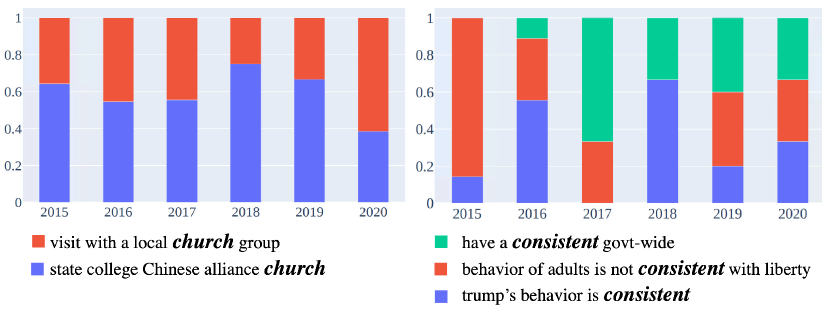
Figure 1: Examples of lexical semantic change across time, where the semantic of word church is stable as it often refers to a building or a local congregation for Christian religious activities. However, the semantic of word consistent varies dramatically at different times.

To better understand and solve the temporal misalignment problem, a series of studies have been launched on pre-trained language models (PLMs) and downstream tasks. The analysis on PLMs Lazaridou et al. (2021) revealed that PLMs (even with larger model sizes) encounter a serious temporal generalization problem, and the misalignment degree increases with time. They also found that continually pre-training PLMs with up-to-the-minute data does mitigate the temporal misalignment problem but suffers from catastrophic forgetting and massive computational cost since further pre-training the converged PLMs is as difficult as pre-training from scratch. The study on downstream tasks further indicates that temporal adaptation (i.e., continually pre-training with unlabelled data that is mostly overlapped in time), while effective, has no apparent advantages over domain adaptation Röttger and Pierrehumbert (2021) (i.e., continually pre-training with domain-specific unlabelled data) and fine-tuning on task-specific data from the target time Luu et al. (2021).

To analyze the reason behind the limited performance of temporal adaptation, we launch a study from the lexical level, which also matches the token-level masking operation in advanced PLMs. Unlike existing research that launches analysis on part-of-speech (POS), topic words, and newly emerging words, we mainly explore the correlations between language model performance and tokens/words with salient lexical semantic change, which is also an extensively studied concept in computational linguistics Dubossarsky et al. (2015); Hamilton et al. (2016); Giulianelli et al. (2020) to investigate how the semantics of words change over time. Experimental results demonstrate that tokens/words with salient lexical semantic change do contribute much more than the rest of tokens/words to the temporal misalignment problem, manifested as their significantly higher perplexity (ppl.) over randomly sampled tokens from the target time. However, the widely-adopted masked language model (MLM) objective in state-of-the-art PLMs uniformly deals with each token/word, letting the salient lexical-level semantic change information over time being overwhelmed by other tokens/words, which can also explain why temporal adaptation has no obvious advantage compared with domain adaptation.

Based on the above findings, we propose a lexical-based masked Language Model (LMLM) objective to capture the lexical semantic change between different temporal splits. Experimental results demonstrate that our proposed method yields significant performance improvement over domain adaptation methods on two different PLMs and four benchmark datasets. Extensive studies also show that LMLM is effective when utilizing different lexical semantic change metrics.

In a nutshell, our contributions are shown below:

• We empirically study the temporal misalignment of PLMs at the lexical level and reveal that the tokens/words with salient lexical semantic change contribute much more to the misalignment problem than other tokens/words. We also disclose that such lexical temporal misalignment information can be overwhelmed by the masked language model training objective of PLMs, resulting in limited performance improvement over temporal and domain adaptation methods.

• We propose a simple yet effective Lexical-based Masked Language Model (LMLM) objective to improve the temporal generalization of PLMs.

• Experiments on two PLMs and four different benchmark datasets confirm that our proposed method is extensively effective in addressing the temporal misalignment problem for downstream tasks, which can significantly outperform existing temporal and domain adaptation methods.

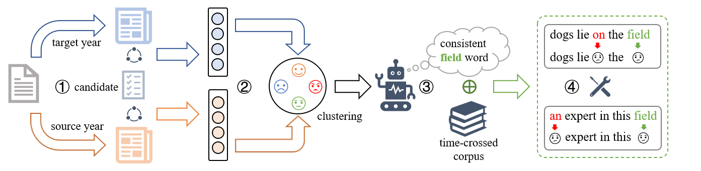
Figure 2: The pipeline of detecting semantic change words (①$\sim$ ③) and the Lexical-based Masked Language Model (LMLM) objective (④). In step ④, the words colored with red are randomly sampled and the words with salient semantic change are colored with green. ALL colored words/tokens are masked during the pre-training stage.

2 Linking Temporal Misalignment with Lexical Semantic Change

Recent work on temporal adaptation Röttger and Pierrehumbert (2021) has found that post-tuning the converged PLMs with unlabeled time-specific data by reusing the MLM objective can make the PLMs perceive related event-driven changes in language usage. Such adaptation can achieve decent performance because the widely-adopted MLM objective can capture the overall changes in the data distribution by randomly masking a specific ratio of the whole sequence. However, such a training objective makes the lexical-level temporal information ignored or overwhelmed by the time-agnostic tokens/words, resulting in little to no performance superiority over domain adaptation methods. Based on the above background, it is natural to explore the role of lexical-level temporal information in temporal adaptation, i.e., whether these tokens/words with salient lexical-semantic changes over time impair the temporal adaptation performance. As a result, we launch a thorough study from the perspective of lexical semantic change to figure out the reason behind the limited performance of temporal adaptation in the specific domain. To the best of our knowledge, this is the first study that explores the correlation between the lexical-semantic change and the temporal adaptation of PLMs. We will firstly illustrate our methods to find those semantic changed words in Section 2.1 and introduce the discovery experiment as well as analyze the results in Section 2.2.

2.1 Lexical Semantic Change Detection

To obtain the semantic changed words, we design a lexical semantic change detection process. For better illustration, we decompose the process into three steps: candidate words selection, feature extraction & Clustering, and semantic change quantification, which are correspond with the step ①$\sim$ ③ in Figure 2.

Candidate Words Selection

Before obtaining the representation of each word, we sample a certain number of candidate words $\mathcal{W}^{t}=\{w_{1}^{t},w_{2}^{t},\cdots,w_{k}^{t}\}$ from the texts $\mathcal{D}^{t}$ of time $t$. Considering that different texts have different domains (politics, culture, history), most keyword extraction methods either heavily rely on dictionaries and a fussy training process Witten et al. (2005); Rose et al. (2010) or are too simple to handle such intricate domain changes, i.e., TF-IDF Ramos et al. (2003). Instead, we turn to YAKE! Campos et al. (2018), a feature-based and unsupervised system to extract keywords in one document. Since the goal is to measure the lexical semantic change among different time splits, we further filter the $\mathcal{W}^{t}$ by calculating the number of the candidate words in different periods and removing the words that are repetitive, too few, or have no real meanings, e.g., pronouns, particles, mood words, etc.

Feature Extraction and Clustering

Given a word $w_{i}$ and one text $d_{i}^{t}=(t_{1},\cdots,t_{i},\cdots,t_{n})$, where $d_{i}^{t}\in\mathcal{D}^{t}$ and $t_{i}=w_{i}$, we utilize a pre-trained language model BERT Devlin et al. (2019) to contextualise each text as the representation $r_{i}^{t}$. Specifically, we look up the sentences in $\mathcal{D}^{t}$ which contain the same candidate words in $\mathcal{W}^{t}$ and feed them into BERT to extract the corresponding word representations followed by aggregating them together Giulianelli et al. (2020). It is worth noting that we extract the representations from the last layer of the BERT model in all experiments, but we also consider extracting the features from the shallow layers of the BERT model. More details can be referred to in Appendix E.

To prevent too much information brought by the long sequences overwhelming the meaning of the candidate words, we specify 128 as the size of occurrence window around the word $w_{i}$, i.e., truncating the redundant part of each sentence. After obtaining $N$ usage representations for each word, we combine them together as representation matrix $\mathcal{R}_{i}^{t}=(r_{1}^{t},r_{2}^{t},\cdots,r_{N}^{t})$ and normalise it.

To distinguish the different semantic representations of each word, we utilize the $K$-Means algorithm, which can automatically cluster the similar word usage type into $K$ groups after $p$ turns according to the representation matrix of each word. Details about the $K$-Means algorithm is elaborated in Appendix A. After clustering, we count the number of sentences in each cluster and calculate the frequency distribution for the candidate word $w_{i}$. When normalized, the frequency distribution can be viewed as the probability distribution $p^{t}_{i}$ over usage types for the candidate word $w_{i}$ at the time $t$. To meet our temporal settings, we should get the probability distributions for the same candidate word in different periods for comparison.

Semantic Change Quantification

To measure the difference between the probability distributions $p^{t}_{i}$ and $p^{t^{\prime}}_{i}$ of the same candidate words in different periods over word usages, we utilize the Jensen-Shannon divergence Lin (1991) metric:

$${\rm JSD}(p^{t}_{i},p^{t^{\prime}}_{i}) =\mathbb{H}\left[\frac{1}{2}(p^{t}_{i}+p^{t^{\prime}}_{i})\right]$$ (1)

$$-\frac{1}{2}\left[\mathbb{H}(p^{t}_{i})-\mathbb{H}(p^{t^{\prime}}_{i})\right],$$

where $\mathbb{H}$ is the Boltzmann-Gibbs-Shannon entropy Ochs (1976). High JSD represents the different frequency distributions, i.e., significant lexical semantic change of the word $t_{i}$, and visa versa. We utilize a hyper-parameter $k$ to control the degree of the lexical semantic change. Specifically, we rank the candidate words according to their JSD values and sample the top-$k$ words as the salient semantic changed words. Several other metrics can also quantify the lexical semantic change, e.g., Entropy Difference (ED) Nardone (2014) and Average pairwise distance (APD) Bohonak (2002), and we will compare the performance among them below.

2.2 Discovery Experiment & Analysis

To highlight the influence of the salient semantic changed words, we design a special masked language modeling objective LMLM, which first masks the candidate words $\mathcal{W}^{t}$ in the texts. Details of the LMLM objective are elaborated in section 3. All the experiments in this section are conducted with the ARXIV dataset, which contains the abstracts of five subjects in different periods, e.g., CS, Math, etc. We apply the pre-trained BERT-base model which has been pre-trained on a large corpus and evaluate it with the latter-released testing sets by reporting the Perplexity (ppl.) value. All the above data are tokenized with Moses, and non-English documents are removed.

Influence of the Semantic Changed Tokens

For comparison, we introduce four masking strategies: random masking, frequency masking, importance masking, and LMLM. The masking ratio of the strategies above is 15%. The random masking strategy, as mentioned above, masks the tokens in the texts randomly, while the frequency masking strategy masks the tokens according to the lexical occurrence frequency, and the importance masking strategy masks the tokes according to the YAKE! scores. Details of the masking strategies are illustrated in Appendix B. The results are shown in the figure 3. We can observe that the ppl. of the LMLM (blue dotted curve) is much higher than the others, which indicates that it is hard for the PLM to predict the lexical semantic changed tokens. The rising trend of four curves shows that the PLM performs increasingly worse when predicting future utterances further away from their training period.

Influence of the Quantification Metric

Furthermore, We utilize three current popular metrics: Jensen-Shannon divergence (JSD), Entropy Difference (ED), and Average Pairwise Distance (APD) to measure the semantic change. The results are shown in the figure 3. Since the slope of the red curve (JSD) is much higher than the others, which means the candidate words selected with the JSD metric are hard to predict, i.e., the semantic change phenomenon of those words is more significant, we apply the JSD metric in the later experiments to find the candidate words $\mathcal{W}^{t}$.

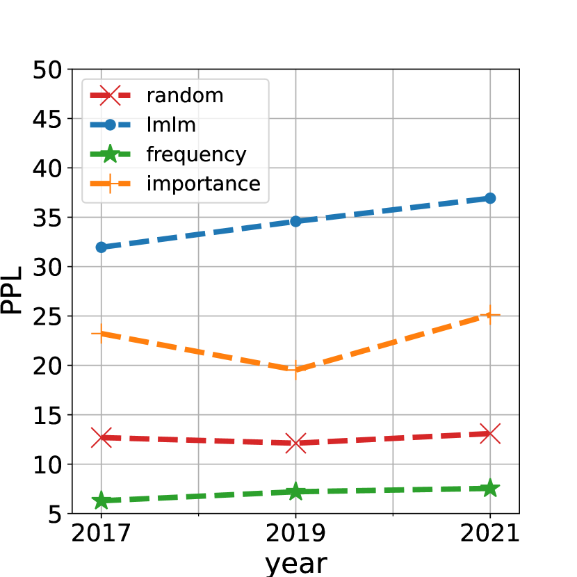
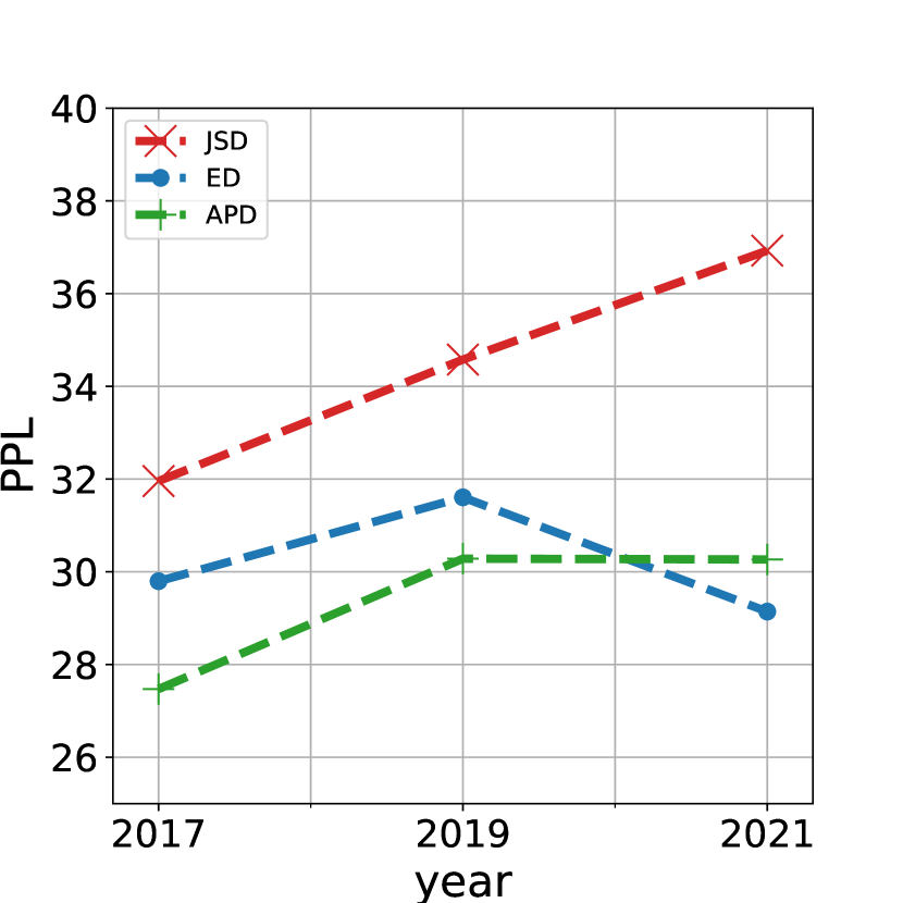
Figure 3: Results of the ppl. value. Figure (a) and (b) shows the effect of the semantic changed words and the results of different quantification metrics respectively.

3 LMLM Objective

Masked Language Model (MLM) objective is a widely-adopted unsupervised task proposed by BERT Devlin et al. (2019), which randomly masks proportional tokens and predicts them. Since the degradation of the PLM in a specific domain over time is mainly attributed to the words with salient semantic change, we should make the PLM more aware of them. Thus, we propose our Lexical-based Masked Language Model (LMLM) objective. Contrary to the traditional random masking strategy (MLM), LMLM preferentially masks the words with salient semantic change over time. Formally, given the text set $\mathcal{D}^{t}=\{d_{1}^{t},d_{2}^{t},\cdots,d_{n}^{t}\}$ at time $t$, we select the candidate words $\mathcal{W}^{t}$ with the aforementioned detection method and rank them according to their JSD value. Then, we select $k~{}(k\in\{100,200,\cdots,1000\})$ words which have relative high scores as the masking candidates $\mathcal{W}_{mask}^{t}$. Given masking ratio $\alpha$, LMLM firstly selects the words in the $\mathcal{W}_{mask}^{t}$ to mask. If there are not enough candidates to meet the total number of masking tokens, LMLM masks the other words in the text randomly. The whole process is corresponding to the step ④ in Figure 2. Assuming it masks $m$ tokens in total and the sentence after masking is $d_{i}^{t^{\prime}}$. The optimization objective of LMLM can be formulated as:

$$\mathcal{L}_{\mathrm{LMLM}}=-\sum\limits_{j=1}^{m}\log P(x=w_{j}|d_{i}^{t^{\prime}};\theta).$$ (2)

4 Experiments

We conduct experiments on the classification task by employing the pre-trained BERT model implemented with the Hugging-Face transformers package in all experiments. Further details about model training and parameters can be found in Appendix C. We will introduce the datasets and the time-stratified settings in Section 4.1, the baselines in Section 4.2, and show the results in Section 4.3.

Dataset	Usage	Time	#Sentences
ARXIV	Fine.	2007$\sim$2019 $\dagger$	160,000
	Pre.	2021	3,800,000
PoliAff	Fine.	2015, 2016	10,000
	Pre. $\ddagger$	2017	1,000,000
RTC	Fine.	Apr. 2017	20,000
	Pre.	Apr. 2018	2,000,000
	Pre.	Aug. 2019	2,000,000

Table 1: Statistics of the datasets, where the time splits of the ARIXV fine-tuning data (marked with $\dagger$) is on a four-year cycle, and the pre-training data of PoliAff dataset (marked with $\ddagger$) is WMT17.

4.1 Basic Settings

Datasets

To ensure the PLM is trained with the data in the specific domain, we select the data with the same or similar distributions between the upstream and downstream stages. We choose the ARXIV dataset for the scientific domain and Reddit Time Corpus (RTC) dataset for the political domain. We also turn to two different datasets with a similar distribution for pre-training and fine-tuning, respectively. Specifically, we select WMT News Crawl (WMT) dataset, which contains news covering various topics, e.g., finance, politics, etc, as unlabeled data and PoliAff dataset in politic domain as labeled data.

Time-Stratified Settings

Generally, the PLM is adapted to temporality using unlabelled data, fine-tuned with the downstream labeled data, and then evaluated with the testing data which has the same time as the pre-training data. We set the $k$ as 500 in all experiments. As for the ARXIV dataset, we utilize the unlabeled data in 2021 for pre-training and extract five years of data from 2011 to 2019 on a four-year cycle for fine-tuning as well as the data in 2021 for testing. Similarly, we collect the data in 2015 and 2016 from the PoliAff dataset as the fine-tuning data and test the model with the data in 2017. For the RTC dataset, we follow the previous work Röttger and Pierrehumbert (2021) to select the unlabeled News Comments dataset for post-training and the political subreddit subset for fine-tuning. However, the number of masking candidates $k$ is less than 500 in most RTC fine-tuning sets of different time splits, which could make the LMLM strategy be regarded as the random masking strategy. Thus, we select the data in April 2017 for fine-tuning (where $k\geq 500$ in this subset) and the data in April 2018 and August 2019 for testing. Detailed data statistics are shown in Table 1.

4.2 Baselines

To meet the time-stratified settings, we select the temporal adaptation TAda method Röttger and Pierrehumbert (2021) as baseline, which first incorporates the temporal information into the PLM by utilizing the time-specific unlabeled data for pre-training and then adapt the PLM to the downstream task with the supervised data. Besides the temporal adaptation method, we also turn to some up-to-date domain adaptation methods since previous work Röttger and Pierrehumbert (2021) points out that such method can mitigate the temporal misalignment problems to some extent. Specifically, we select PERL Ben-David et al. (2020) and DILBERT Lekhtman et al. (2021) methods, and implement them under the time-stratified settings. Details of the domain adaptation methods are shown in the Appendix D. We calculate the F1 score as the testing results for all the experiments.

Method	Fine-tuning Data
	2007	2011	2015	2019	Avg.
TAda	82.97	84.72	84.82	84.99	84.38
+ PERL	75.67	79.20	78.89	78.77	78.13
+ DILBERT	82.62	83.89	84.04	84.22	83.69
+ LMLM	84.93	86.52	86.49	87.22	86.29

Table 2: Results of the ARXIV dataset.

Method	Fine-tuning Data
	2015	2016	Avg.
TAda	66.05	72.94	69.50
+ PERL	61.79	68.21	65.00
+ DILBERT	63.89	69.86	66.88
+ LMLM	67.00	74.10	70.55

Table 3: Results of the PoliAff dataset.

4.3 Main Results

ARXIV Dataset

The results of the ARXIV dataset are shown in Table 2, and we can observe that applying domain adaptation methods under the time-stratified settings aggravate the temporal misalignment problem as the scores of the PERL and DILBERT methods are not as high as those for utilizing the TAda directly. However, the performance of LMLM is much better than the other three methods.

PoliAff Dataset

We report the results of the PoliAff dataset in Table 3. Although there is a slight domain difference between the pre-training and fine-tuning data, i.e., news and politic, the LMLM can still achieve the best results, and the domain adaptation methods still perform worse than the temporal adaptation methods.

RTC Dataset

The results of the RTC dataset is shown in Table 4, and we can find the similar tendency as the previous results, i.e., LMLM still achieve the best performance. However, the differences among the four methods in RTC dataset are much smaller compared with the previous results, which is largely due to the slight dynamic temporality of the RTC dataset.

Method	Testing Data
	Apr. 2018	Aug. 2019	Avg.
TAda	41.78	38.14	39.96
+ PERL	40.21	37.14	38.68
+ DILBERT	42.99	38.20	40.60
+ LMLM	43.91	39.38	41.65

Table 4: Results of the RTC dataset.

5 Study

In this section, we conduct extensive studies to help better understand our method. It is worth noting that all the experiments in this section are conducted on the BERT model with the ARXIV dataset unless there is a clear explanation.

5.1 Effect of Pre-training Data Selection

To explore the temporal impact brought by pre-training data, we launch experiments with MLM objective under two different pre-training settings:

• Source Year Consistent Pre-training (SYCP) We keep the time of pre-training data consistent with that of fine-tuning data to ensure the consistency between the two stages.

• Target Year Consistent Pre-training (TYCP) Following the previous work Röttger and Pierrehumbert (2021); Lazaridou et al. (2021), we utilize the pre-training data in consistent with the evaluation data in temporal dimension, i.e., the time of pre-training data and evaluation data is same.

We also implement our LMLM objective in the pre-training stage for comparison, where the masking ratio is 15%, and $k$ is 1000. The results are shown in the table 5. We can find that the performance of SYCP gradually overwhelms the TYCP as the time passes towards the target year. When the PLM is pre-trained with MLM objective under the SYCP setting, it can even outcome the performance of TYCP, and the PLM pre-trained with LMLM objective under the TYCP setting can achieve the best performance. On the one hand, we can infer that the temporal adaptation method is effective since TYCP beats the SYCP. On the other hand, the LMLM objective can make the PLM pay more attention to the salient semantic changed words as pre-training with the LMLM objective under the SYCP settings (SYCP+LMLM) can even surpass the original temporal adaptation method (TYCP).

Method	Fine-tuning Data
	2007	2011	2015	2019	Avg.
SYCP	82.81	84.62	85.54	85.17	84.54
TYCP (TAda)	82.97	84.72	84.82	84.99	84.38
SYCP + LMLM	83.52	85.41	86.36	87.03	85.58
TYCP + LMLM	84.93	86.52	86.49	87.22	86.29

Table 5: Results of different pre-training strategies.

5.2 Hyper-Parameter Analysis

Since there is a strong relationship between the masking ratio and the model’s performance, we conduct experiments to look for the best masking strategy for the LMLM objective. Furthermore, we also want to know whether the temporal misalignment problem can be better mitigated by masking more salient semantic changed words. Thus, we select the data in 2021 for pre-training with our LMLM objective and the data in 2009 for fine-tuning, followed by testing the model with the data in 2021. For better comparison, we utilize a heat map (Figure 4) to display the results, where the vertical axis of this graph represents the masking ratio $\alpha$, and the horizontal axis represents the number of masked salient semantic changed words $k$.

The Influence of $\alpha$

We calculate the average value of the results of each masking ratio under different settings of $k$ and observe that when the masking ratio is around 30%, the PLM can achieve the best performance.

JSD ($\uparrow$)	#Sen	Prec.	SeC.
0.00$\sim$0.05	902	90.2%	micro
0.05$\sim$0.10	78	7.8%	medium
0.10$\sim$0.15	18	1.8%	great
0.15$\sim$0.2	2	0.2%	great

Table 6: Distribution of the semantic changed words, where SeC. represents for the Semantic Change.

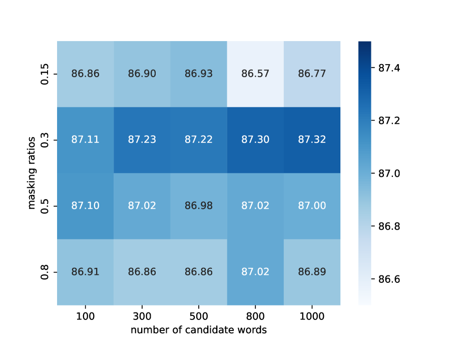
Figure 4: Results of the different masking strategies of LMLM. The horizontal axis indicates the number of masked semantic changed words $k$ and the vertical axis represents for the masking ratio $\alpha$.

The Influence of $k$

No doubt forcing the model to predict more high semantic change words can better mitigate the temporal problem generally. However, it is surprising to observe that the improvement is slight across different settings of $k$. Thus, we quantify the semantic change of 1,000 random sampled words from the candidates $\mathcal{W}^{t}_{mask}$ according to the JSD value and the distribution of those words is shown in Table 6. We can find that only around $10\%$ words have relative significant semantic change (JSD value $\geq 0.05$) while around $72\%$ words have little or no semantic change (JSD value $\approx 0.00$). We can conclude that the improvement mainly comes from predicting a few keywords, i.e., topic words and newly emerging words, which have relatively salient semantic change.

5.3 Pre-trained Language Model Analysis

To verify the generalization of our methods on different PLMs, we implement our method on two PLMs, i.e., BERT and RoBERTa, and utilize the temporal adaptation method Röttger and Pierrehumbert (2021) as the baseline for comparison. As shown in table 7, we find there is a dramatic improvement of each PLM, i.e., 1.42 points improvement of the BERT model and 0.48 points improvement of the RoBERTa model on average.

PLMs	Fine-tuning Data
	2007	2011	2015	2019	Avg.
BERT	82.97	84.72	84.82	84.99	84.38
+ TSC-Ada	84.93	86.52	86.49	87.22	85.80
RoBERTa	81.72	84.37	84.46	84.95	83.88
+ TSC-Ada	82.32	84.92	84.59	85.40	84.36

Table 7: Results of different PLMs under the time-stratified settings.

Metrics	Fine-tuning Data
	2007	2011	2015	2019	Avg.
ED	84.99	86.62	86.43	87.60	86.41
APD	85.02	86.34	86.24	87.08	86.17
JSD	84.93	86.52	86.49	87.22	86.29

Table 8: Results of different quantification metrics.

Method	Fine-tuning Data
	2014	2015	2016	Avg.
TAda	81.23	80.91	81.94	81.36
+ LMLM	81.41	82.50	82.63	82.18

Table 9: Results of the CoNLL dataset.

Settings	2007		2011		2015		2019
	LMLM	TAda	LMLM	TAda	LMLM	TAda	LMLM	TAda
Results (Total)	84.32	82.27	86.28	84.60	86.17	85.13	87.17	85.18
Results (w/o Temp)	83.81	81.80	85.99	83.84	86.38	85.68	87.60	85.99
Results (w/ Temp)	84.02	82.79	86.40	84.97	85.62	84.30	86.66	84.35
Mask (Failed Sets)	12.87	12.91	10.75	11.25	8.95	9.96	10.41	13.04
PAD (Failed Sets)	12.62	13.34	11.15	11.02	8.81	10.14	10.58	12.77
REP (Failed Sets)	13.58	13.23	10.89	11.75	8.81	9.78	9.92	13.57

Table 10: Error analysis of the LMLM method, where the first group shows the results on the hierarchical data (w/ and w/o temporal information) while the second group shows the results on the failed examples.

5.4 Quantification Metrics

As mentioned above, there are several metrics to quantify the semantic change, and we primarily conduct the experiment to select the JSD metric and we compare three commonly used metrics, i.e., ED, APD, and JSD, in this section. As shown in the table 8, we can find that although different metrics have their advantages, the differences among them are slight. For example, the maximum difference is 0.24 points among three metrics on average.

5.5 Open-Domain Temporal Adaptation

As mentioned above, we conduct all the experiments under the domain-specific setting. In this section, we explore the effect of the LMLM objective with the name entity recognition task under the open-domain setting, i.e., the downstream dataset has no specific domain. Specifically, we select the WMT dataset in 2017 as the unlabeled data and the subset in 2015 and 2016 from the CoNLL dataset as the fine-tuning data. In the end, we evaluate the model with the data in 2017. The results are shown in Table 9. We can find that the LMLM method outperforms the original temporal adaptation method with around 1 point improvement.

5.6 Error Analysis

We also conduct fine-grained experiments to study why our method fails with some examples. Specifically, we utilize the ARXIV dataset from 2007 to 2017 to fine-tune the model and the data in 2021 for testing. We first select the top 100 lexical semantic changed tokens for each testing set. Then, we divide the testing data into two parts: a subset with temporal information and a subset without temporal information by judging whether the texts contain the selected tokens. As shown in the first group of Table 10, the LMLM method can achieve better results than TAda on both testing subsets, and the improvement on the subset with temporal information is more significant than that on the subset without the temporal information. A possible explanation for why LMLM performs better on the subset without temporal information is that there is still some temporal information left in this data since we distinguish the subset with only 100 lexical semantic changed tokens.

Besides, we collect the failed testing sets, i.e., the model predicting wrong labels on those data, and mask those mentioned above top 100 lexical semantic changed tokens in the texts with two strategies: (1) replace those tokens with special placeholder <MASK> or <PAD>, and (2) randomly utilize other tokens in the vocabulary (except the aforementioned lexical semantic changed tokens) for substitution. The results are shown in the second group of Table 10, where we can observe that TAda surpasses our method in general. We think those masked/replaced lexical semantic changed tokens, which LMLM pays more attention to, may be the critical messages for the model to help the decision. The missing of that important information can cause a negative impact on the model, which leads to the performance decreasing.

6 Related Work

6.1 Temporal Misalignment

Previous studies have shown that models trained on texts from one time period perform poorly when tested on texts in later periods for NLP tasks like machine translation Levenberg et al. (2010), review and news article classification Huang and Paul (2019, 2018), named entity recognition Rijhwani and Preoţiuc-Pietro (2020) and so on. Within the current paradigm of using PLMs Devlin et al. (2019), studies have focused more on the expansion of dataset Liu et al. (2019); Lewis et al. (2020); Yang et al. (2019) and model capacity Raffel et al. (2019); Lan et al. (2019); Brown et al. (2020) to achieve better performance but ignore the temporal effects. Few studies focus on such problem, Lazaridou et al. (2021) have empirically studied the degraded performance of PLMs over time, and Röttger and Pierrehumbert (2021) focus on post-tuning BERT with the data in specific periods to mitigate the temporal misalignment problems. Furthermore, Amba Hombaiah et al. (2021) propose sampling methods to help PLMs achieve better performance on the evolving content. In this paper, we conduct a detailed investigation from the perspective of lexical semantic change to figure out the reason behind the limited performance of the PLMs under the time-stratified settings.

6.2 Lexical Semantic Change

Lexical semantic change is an extensively studied concept in the computational linguistics, which mainly focuses on deciding whether the concept of a word has changed over time (semantic change detection) Gulordava and Baroni (2011); Kulkarni et al. (2015); Dubossarsky et al. (2015); Hamilton et al. (2016) or discovering the instances with high semantic change (semantic change discovery) Hengchen et al. (2021); Kurtyigit et al. (2021); Jatowta et al. (2021). Among them, most studies utilize contextualized word representations Turney and Pantel (2010); Giulianelli et al. (2020) and measure the distance among them in different periods Cook and Stevenson (2010); Gulordava and Baroni (2011); Hamilton et al. (2016) to detect or discover the instances with salient semantic change. Previous studies mainly concentrate on applying PLMs to discover the semantic change phenomena, while our work focuses on solving such problems intrinsic in the PLMs. Thus, besides observing such semantic changed phenomenon, we aim to find the corresponding words and apply the LMLM objective to make the PLMs more aware of them to mitigate the temporal misalignment problem. Most studies focused on obtaining those words are under the supervised settings Kim et al. (2014); Basile et al. ; Basile and McGillivray (2018); Tsakalidis et al. (2019) by scoring and selecting the top-ranked words through author intuitions or known historical data Kurtyigit et al. (2021). While Giulianelli et al. propose one unsupervised method, adding one clustering process to the traditional selecting methods. To our best knowledge, this is the first work that links semantic change with temporal adaptation.

7 Conclusion & Future Work

In this paper, we investigate the temporal misalignment of the PLMs from the lexical level and observe that the words with salient lexical semantic change contribute significantly to the temporal problems. We propose a lexical-based masked Language Model (LMLM) objective based on the above observation. Experiments on two PLMs with the sequence classification task on three datasets under the specific domain setting and one name entity recognition task under the open-domain setting confirm that our proposed method performs better than the previous temporal adaptation methods and the state-of-the-art domain adaptation methods. In the future, we will keep discovering such temporal misalignment problems in the text generation tasks, e.g., machine translation, and improve our method by reducing the extra offline computational cost on procedures like Semantic Change Detection.

8 Limitation

There are still some limitations in our work which are listed below:

• The other tokens in the text influence the meaning of the target word to some extent since we utilize sentence contextualization to represent the meaning of the target word. To this end, it is hard to interpret why some candidate words are selected by the detection step, e.g., name entities or numbers, whose meaning remains unchanged. We will design a better unsupervised word selection strategy in the future.

• We utilize the lexical-level masking strategy, while the semantic change can also be reflected with the whole sequence, e.g., the topic of “Malaysia Airlines crashed into the sea” may be one hypothesis before 2014, but it became a severe accident in 2014. Current famous MLM objectives like span masking objective Raffel et al. (2020) or sentence masking objective Tay et al. (2022) have observed that the performance of denoising the whole sequence is better than denoising the single token in some NLU tasks. In the future, we will explore whether the sequence masking objective mentioned above can mitigate the temporal misalignment problem inherent in the PLMs.

Appendix A Implementation of the K-Means Algorithm

Given a representation matrix $\mathcal{R}^{t}_{i}=\{r^{t}_{i}\}_{i\in(1,\cdots,N)}$ for the word $w^{t}_{i}$ we utilize the silhouette score Rousseeuw (1987) to obtain the optimal $K$ for K-Means algorithm. We experiment with $K\in[2,10]$ in a heuristic way. For each $K$, the clustering result is the one that yields the minimal distortion value, i.e., the minimal sum of squared distances of each data point from its closest centroid, and we execute ten iterations to alleviate the influence of different initialization values Vassilvitskii and Arthur (2006). Since there are several monosemous words, i.e., the number of $K$ is 1, we filter those words with a threshold $d$. Specifically, if the intra-cluster dispersion value of a word is below $d$, we would allocate $K=1$, otherwise, $K\geq 2$. The optimal $K$ is the one that can simultaneously minimize the dispersion score and maximize the silhouette score.

Appendix B Implementation of the Masking Strategies

In this section, we illustrate the frequency masking strategy and importance masking strategy in detail. Given a dataset that contains $n$ texts, we firstly utilize the NLTK tool to tokenize each text and follow the below processes:

Frequency Masking Strategy

We add each tokenized token into the dictionary $\mathcal{D}$ and record the number of its occurrence. We sort the tokens in $\mathcal{D}$ according to the occurrence times and select the tokens to mask in descending order until the masking ratio is satisfied.

Importance Masking Strategy

We utilize the YAKE! method as mentioned above to sort the tokenized tokens according to the scores calculated with the task label, e.g., the label of CS in the ARXIV dataset. Finally, we select the tokens to mask in descending order until the masking ratio is satisfied.

Appendix C Model Training & Parameters

Architecture

We utilize the BERT-base uncased model pretrained on a large corpus of English data with the MLM objective. The model contains 12 transformer layers, 12 attention heads, and the hidden layer size is 768. The total number of parameters is 110 million. We add a linear layer after the last BERT layer for the downstream classification task and generate the output with softmax. The maximum input sequence length is 512.

Training Details

We utilize cross-entropy loss in the pre-training and fine-tuning stages and apply AdamW Loshchilov and Hutter (2017) as the optimizer. Specifically, the learning rate is 5e-5, and the weight decay is 0.01. Moreover, we set a 10% dropout probability for regularisation, We pre-train the model for one epoch and fine-tune the model until convergency. We set the batch size as 128 and conduct the experiments on eight NVIDIA GTX3090 GPUs.

Evaluation Metric

We utilize the F1 score as the evaluation metric in all the experiments.

Appendix D Implementation of the Baselines

This section will elaborate on how to apply the domain adaptation methods under the temporal adaptation settings.

PERL

Ben-David et al. (2020) This method model parameters using a pivot-based  Blitzer et al. (2006, 2007) variant of the MLM object with unlabeled datasets from both the source and target temporal split. Instead of masking each token with the same probability, we divided token into pivots and non-pivots to learn the pivot/non-pivot distinction on unlabeled data from the source and target time span. The encoder weights are frozen during training for the downstream task. Specifically, we rank those frequent features (occurs at least 20 times in the unlabeled data from the source and target time split) based on the mutual information with the task label according to source domain labeled data. Then, we select top 100 which have relative high scores as pivot features. The non-pivot feature subset consists of features that do not match the two requirements.

DILBERT

Lekhtman et al. (2021) is the SOTA in Aspect Extraction while using a fraction of the unlabeled data. Different from PERL, they challenge the “high MI with the task label" criterion in the pivot definition. In our settings, we harness the information about the golden label(physics, cs., etc) in the source and target temporal split to mask words that are more likely to bridge the gap between the different periods. Specifically, we compute the cosine similarity between each input word and the label from both the source and the target. We keep the highest similarity score for each word and mask the top 0.15% of the input words. For the downstream task, they add a logistic regression head on top of all outputs and fine-tune the model on the source period labeled data.

Appendix E Feature Extracting

One point that worth discussing is the hidden states from the last layer of the BERT model ($\mathrm{LMLM_{\texttt{LAST}}}$) contains massive amounts of contextual information, which may overwhelm the lexical information. Thus we turn to the representation from the shallow layer of the BERT model, e.g., representation from the second BERT layer ( $\mathrm{LMLM_{\texttt{SECOND}}}$). Specifically, we conduct the experiment on the ARXIV testing set in 2013, and the results are shown in Table 11.

Model	F1
$\mathrm{LMLM_{\texttt{LAST}}}$	87.45
$\mathrm{LMLM_{\texttt{SECOND}}}$	86.67
TAda	85.04

Table 11: Results on the ARXIV testing set.

As we can observe from the table that the $\mathrm{LMLM_{\texttt{SECOND}}}$ can achieve a better result than TAda, which indicates that the representations from the earlier layer are strong enough to help achieve a decent performance improvement. Besides, the $\mathrm{LMLM_{\texttt{LAST}}}$ achieves a better result than $\mathrm{LMLM_{\texttt{SECOND}}}$, which means that the hidden states which contain sentence-level information can help promote the accuracy in the detection process.

References

- Amba Hombaiah et al. (2021) Spurthi Amba Hombaiah, Tao Chen, Mingyang Zhang, Michael Bendersky, and Marc Najork. 2021. Dynamic language models for continuously evolving content. In Proceedings of the 27th ACM SIGKDD Conference on Knowledge Discovery & Data Mining, pages 2514–2524.
- Bamler and Mandt (2017) Robert Bamler and Stephan Mandt. 2017. Dynamic word embeddings. In International conference on Machine learning, pages 380–389. PMLR.
- (3) Pierpaolo Basile, Annalina Caputo, Roberta Luisi, and Giovanni Semeraro. Diachronic analysis of the italian language exploiting google ngram.
- Basile and McGillivray (2018) Pierpaolo Basile and Barbara McGillivray. 2018. Exploiting the web for semantic change detection. In International Conference on Discovery Science, pages 194–208. Springer.
- Ben-David et al. (2020) Eyal Ben-David, Carmel Rabinovitz, and Roi Reichart. 2020. Perl: Pivot-based domain adaptation for pre-trained deep contextualized embedding models. Transactions of the Association for Computational Linguistics, 8:504–521.
- Blitzer et al. (2007) John Blitzer, Mark Dredze, and Fernando Pereira. 2007. Biographies, bollywood, boom-boxes and blenders: Domain adaptation for sentiment classification. In Proceedings of the 45th annual meeting of the association of computational linguistics, pages 440–447.
- Blitzer et al. (2006) John Blitzer, Ryan McDonald, and Fernando Pereira. 2006. Domain adaptation with structural correspondence learning. In Proceedings of the 2006 conference on empirical methods in natural language processing, pages 120–128.
- Bohonak (2002) AJ Bohonak. 2002. Ibd (isolation by distance): a program for analyses of isolation by distance. Journal of Heredity, 93(2):153–154.
- Brown et al. (2020) Tom Brown, Benjamin Mann, Nick Ryder, Melanie Subbiah, Jared D Kaplan, Prafulla Dhariwal, Arvind Neelakantan, Pranav Shyam, Girish Sastry, Amanda Askell, et al. 2020. Language models are few-shot learners. Advances in neural information processing systems, 33:1877–1901.
- Campos et al. (2018) Ricardo Campos, Vítor Mangaravite, Arian Pasquali, Alípio Mário Jorge, Célia Nunes, and Adam Jatowt. 2018. Yake! collection-independent automatic keyword extractor. In European Conference on Information Retrieval, pages 806–810. Springer.
- Cook and Stevenson (2010) Paul Cook and Suzanne Stevenson. 2010. Automatically identifying changes in the semantic orientation of words. In Proceedings of the Seventh International Conference on Language Resources and Evaluation (LREC’10).
- Del Tredici et al. (2018) Marco Del Tredici, Raquel Fernández, and Gemma Boleda. 2018. Short-term meaning shift: A distributional exploration. arXiv preprint arXiv:1809.03169.
- Devlin et al. (2019) Jacob Devlin, Ming-Wei Chang, Kenton Lee, and Kristina Toutanova. 2019. Bert: Pre-training of deep bidirectional transformers for language understanding. In Proceedings of the 2019 Conference of the North American Chapter of the Association for Computational Linguistics: Human Language Technologies, Volume 1 (Long and Short Papers), pages 4171–4186.
- Dubossarsky et al. (2015) Haim Dubossarsky, Yulia Tsvetkov, Chris Dyer, and Eitan Grossman. 2015. A bottom up approach to category mapping and meaning change. In NetWordS, pages 66–70.
- Giulianelli et al. (2020) Mario Giulianelli, Marco Del Tredici, and Raquel Fernández. 2020. Analysing lexical semantic change with contextualised word representations. arXiv preprint arXiv:2004.14118.
- Gulordava and Baroni (2011) Kristina Gulordava and Marco Baroni. 2011. A distributional similarity approach to the detection of semantic change in the google books ngram corpus. In Proceedings of the GEMS 2011 workshop on geometrical models of natural language semantics, pages 67–71.
- Hamilton et al. (2016) William L Hamilton, Jure Leskovec, and Dan Jurafsky. 2016. Diachronic word embeddings reveal statistical laws of semantic change. In Proceedings of the 54th Annual Meeting of the Association for Computational Linguistics (Volume 1: Long Papers), pages 1489–1501.
- Hengchen et al. (2021) Simon Hengchen, Ruben Ros, Jani Marjanen, and Mikko Tolonen. 2021. A data-driven approach to studying changing vocabularies in historical newspaper collections. Digital Scholarship in the Humanities, 36(Supplement_2):ii109–ii126.
- Huang and Paul (2019) Xiaolei Huang and Michael Paul. 2019. Neural temporality adaptation for document classification: Diachronic word embeddings and domain adaptation models. In Proceedings of the 57th Annual Meeting of the Association for Computational Linguistics, pages 4113–4123.
- Huang and Paul (2018) Xiaolei Huang and Michael J Paul. 2018. Examining temporality in document classification. In Proceedings of the 56th Annual Meeting of the Association for Computational Linguistics (Volume 2: Short Papers), volume 2.
- Jatowta et al. (2021) Adam Jatowta, Nina Tahmasebib, and Lars Borinb. 2021. Computational approaches to lexical semantic change: Visualization systems and novel applications. Computational approaches to semantic change, 6:311.
- Kim et al. (2014) Yoon Kim, Yi-I Chiu, Kentaro Hanaki, Darshan Hegde, and Slav Petrov. 2014. Temporal analysis of language through neural language models. ACL 2014, page 61.
- Kulkarni et al. (2015) Vivek Kulkarni, Rami Al-Rfou, Bryan Perozzi, and Steven Skiena. 2015. Statistically significant detection of linguistic change. In Proceedings of the 24th international conference on world wide web, pages 625–635.
- Kurtyigit et al. (2021) Sinan Kurtyigit, Maike Park, Dominik Schlechtweg, Jonas Kuhn, and Sabine Schulte im Walde. 2021. Lexical semantic change discovery. In Proceedings of the 59th Annual Meeting of the Association for Computational Linguistics and the 11th International Joint Conference on Natural Language Processing (Volume 1: Long Papers), pages 6985–6998.
- Lan et al. (2019) Zhenzhong Lan, Mingda Chen, Sebastian Goodman, Kevin Gimpel, Piyush Sharma, and Radu Soricut. 2019. Albert: A lite bert for self-supervised learning of language representations. arXiv preprint arXiv:1909.11942.
- Lazaridou et al. (2021) Angeliki Lazaridou, Adhi Kuncoro, Elena Gribovskaya, Devang Agrawal, Adam Liska, Tayfun Terzi, Mai Gimenez, Cyprien de Masson d’Autume, Tomas Kocisky, Sebastian Ruder, et al. 2021. Mind the gap: Assessing temporal generalization in neural language models. Advances in Neural Information Processing Systems, 34.
- Lekhtman et al. (2021) Entony Lekhtman, Yftah Ziser, and Roi Reichart. 2021. Dilbert: Customized pre-training for domain adaptation with category shift, with an application to aspect extraction. In Proceedings of the 2021 Conference on Empirical Methods in Natural Language Processing, pages 219–230.
- Levenberg et al. (2010) Abby Levenberg, Chris Callison-Burch, and Miles Osborne. 2010. Stream-based translation models for statistical machine translation. In Human Language Technologies: The 2010 Annual Conference of the North American Chapter of the Association for Computational Linguistics, pages 394–402.
- Lewis et al. (2020) Mike Lewis, Yinhan Liu, Naman Goyal, Marjan Ghazvininejad, Abdelrahman Mohamed, Omer Levy, Veselin Stoyanov, and Luke Zettlemoyer. 2020. Bart: Denoising sequence-to-sequence pre-training for natural language generation, translation, and comprehension. In Proceedings of the 58th Annual Meeting of the Association for Computational Linguistics, pages 7871–7880.
- Lin (1991) Jianhua Lin. 1991. Divergence measures based on the shannon entropy. IEEE Transactions on Information theory, 37(1):145–151.
- Liu et al. (2019) Yinhan Liu, Myle Ott, Naman Goyal, Jingfei Du, Mandar Joshi, Danqi Chen, Omer Levy, Mike Lewis, Luke Zettlemoyer, and Veselin Stoyanov. 2019. Roberta: A robustly optimized bert pretraining approach.
- Loshchilov and Hutter (2017) Ilya Loshchilov and Frank Hutter. 2017. Decoupled weight decay regularization. arXiv preprint arXiv:1711.05101.
- Luu et al. (2021) Kelvin Luu, Daniel Khashabi, Suchin Gururangan, Karishma Mandyam, and Noah A Smith. 2021. Time waits for no one! analysis and challenges of temporal misalignment. arXiv preprint arXiv:2111.07408.
- Nardone (2014) Pasquale Nardone. 2014. Entropy of difference. arXiv preprint arXiv:1411.0506.
- Ochs (1976) W Ochs. 1976. Basic properties of the generalized boltzmann-gibbs-shannon entropy. Reports on Mathematical Physics, 9(2):135–155.
- Radford et al. (2018) Alec Radford, Karthik Narasimhan, Tim Salimans, and Ilya Sutskever. 2018. Improving language understanding by generative pre-training.
- Radford et al. (2019) Alec Radford, Jeffrey Wu, Rewon Child, David Luan, Dario Amodei, Ilya Sutskever, et al. 2019. Language models are unsupervised multitask learners. OpenAI blog, 1(8):9.
- Raffel et al. (2019) Colin Raffel, Noam Shazeer, Adam Roberts, Katherine Lee, Sharan Narang, Michael Matena, Yanqi Zhou, Wei Li, and Peter J Liu. 2019. Exploring the limits of transfer learning with a unified text-to-text transformer. arXiv preprint arXiv:1910.10683.
- Raffel et al. (2020) Colin Raffel, Noam Shazeer, Adam Roberts, Katherine Lee, Sharan Narang, Michael Matena, Yanqi Zhou, Wei Li, Peter J Liu, et al. 2020. Exploring the limits of transfer learning with a unified text-to-text transformer. J. Mach. Learn. Res., 21(140):1–67.
- Ramos et al. (2003) Juan Ramos et al. 2003. Using tf-idf to determine word relevance in document queries. In Proceedings of the first instructional conference on machine learning, volume 242, pages 29–48. Citeseer.
- Rijhwani and Preoţiuc-Pietro (2020) Shruti Rijhwani and Daniel Preoţiuc-Pietro. 2020. Temporally-informed analysis of named entity recognition. In Proceedings of the 58th Annual Meeting of the Association for Computational Linguistics, pages 7605–7617.
- Rose et al. (2010) Stuart Rose, Dave Engel, Nick Cramer, and Wendy Cowley. 2010. Automatic keyword extraction from individual documents. Text mining: applications and theory, 1:1–20.
- Rosenfeld and Erk (2018) Alex Rosenfeld and Katrin Erk. 2018. Deep neural models of semantic shift. In Proceedings of the 2018 Conference of the North American Chapter of the Association for Computational Linguistics: Human Language Technologies, Volume 1 (Long Papers), pages 474–484.
- Röttger and Pierrehumbert (2021) Paul Röttger and Janet Pierrehumbert. 2021. Temporal adaptation of bert and performance on downstream document classification: Insights from social media. In Findings of the Association for Computational Linguistics: EMNLP 2021, pages 2400–2412.
- Rousseeuw (1987) Peter J Rousseeuw. 1987. Silhouettes: a graphical aid to the interpretation and validation of cluster analysis. Journal of computational and applied mathematics, 20:53–65.
- Tay et al. (2022) Yi Tay, Mostafa Dehghani, Vinh Q Tran, Xavier Garcia, Dara Bahri, Tal Schuster, Huaixiu Steven Zheng, Neil Houlsby, and Donald Metzler. 2022. Unifying language learning paradigms. arXiv preprint arXiv:2205.05131.
- Tsakalidis et al. (2019) Adam Tsakalidis, Marya Bazzi, Mihai Cucuringu, Pierpaolo Basile, and Barbara McGillivray. 2019. Mining the uk web archive for semantic change detection. In Proceedings of the International Conference on Recent Advances in Natural Language Processing (RANLP 2019), pages 1212–1221.
- Turney and Pantel (2010) Peter D Turney and Patrick Pantel. 2010. From frequency to meaning: Vector space models of semantics. Journal of artificial intelligence research, 37:141–188.
- Vassilvitskii and Arthur (2006) Sergei Vassilvitskii and David Arthur. 2006. k-means++: The advantages of careful seeding. In Proceedings of the eighteenth annual ACM-SIAM symposium on Discrete algorithms, pages 1027–1035.
- Witten et al. (2005) Ian H Witten, Gordon W Paynter, Eibe Frank, Carl Gutwin, and Craig G Nevill-Manning. 2005. Kea: Practical automated keyphrase extraction. In Design and Usability of Digital Libraries: Case Studies in the Asia Pacific, pages 129–152. IGI global.
- Yang et al. (2019) Zhilin Yang, Zihang Dai, Yiming Yang, Jaime Carbonell, Russ R Salakhutdinov, and Quoc V Le. 2019. Xlnet: Generalized autoregressive pretraining for language understanding. Advances in neural information processing systems, 32.
- Zhang and Li (2021) Min Zhang and Juntao Li. 2021. A commentary of gpt-3 in mit technology review 2021. Fundamental Research, 1(6):831–833.