BOREx: Bayesian-Optimization–Based Refinement of Saliency Map for Image- and Video-Classification Models

Abstract

Explaining a classification result produced by an image- and video-classification model is one of the important but challenging issues in computer vision. Many methods have been proposed for producing heat-map–based explanations for this purpose, including ones based on the white-box approach that uses the internal information of a model (e.g., LRP, Grad-CAM, and Grad-CAM++) and ones based on the black-box approach that does not use any internal information (e.g., LIME, SHAP, and RISE).

We propose a new black-box method BOREx (Bayesian Optimization for Refinement of visual model Explanation) to refine a heat map produced by any method. Our observation is that a heat-map–based explanation can be seen as a prior for an explanation method based on Bayesian optimization. Based on this observation, BOREx conducts Gaussian process regression (GPR) to estimate the saliency of each pixel in a given image starting from the one produced by another explanation method. Our experiments statistically demonstrate that the refinement by BOREx improves low-quality heat maps for image- and video-classification results.

1 Introduction

(a) Input

(b) BOREx (Our method)

(c) RISE

(d) BO

Figure 1: Example of the saliency maps generated by our method BOREx (in column (b)), RISE [17] (in column (c)), and the Bayesian-optimization-based method [16] (in column (d)); the input images to each method are presented in column (a). The classification label used in the saliency maps in each row is “dining table”, “Labrador retriever”, and “folding chair” from the first row.

Many image- and video-classification methods based on machine learning have been developed and are widely used. However, many of these methods (e.g., DNN-based ones) are not interpretable to humans. The lack of interpretability is sometimes problematic in using an ML-based classifier under a safety-critical system such as autonomous driving.

To address this problem, various methods to explain the result of image and video classification in the form of a heatmap called saliency map [28, 17, 21, 5, 22, 10, 16] have been studied. Fig. 1 shows examples of saliency maps synthesized by several methods, including ours. A saliency map for an image-classification result is an image of the same size as the input image. Each pixel in the saliency map shows the contribution of the corresponding pixel in the input image to the classification result. In each saliency map, the part that positively contributes to the classification result is shown in red, whereas the negatively-contributing parts are shown in blue. The notion of saliency maps is extended to explain the results produced by a video-classification model, e.g., in [5] and [23].

These saliency-map generation techniques can be classified into two groups: the white-box approach and the black-box approach. A technique in the former group uses internal information (e.g., gradient computed inside DNN) to generate a saliency map; Grad-CAM [21] and Grad-CAM++ [5] are representative examples of this group. A technique in the latter group does not use internal information. Instead, it repeatedly perturbs the input image by occluding several parts randomly and synthesizes a saliency map based on the change in the outputs of the model to the masked images from that of the original one. The representative examples of this group are LIME [20], SHAP [15], and RISE [17].

Although these methods provide valuable information to interpret many classification results, the generated saliency maps sometimes do not correctly localize the regions that contribute to a classification result [3, 25, 9]. Such a low-quality saliency map cannot be used to interpret a classification result correctly.

Mokuwe et al. [16] recently proposed another black-box saliency map generation method using Bayesian optimization based on the theory of Gaussian processes regression (GPR) [19]. Their method maintains (1) the estimated saliency value of each pixel and (2) the estimated variance of the saliency values during an execution of their procedure, assuming that a Gaussian process can approximate the saliency map; this assumption is indeed reasonable in many cases because a neighbor of an important pixel is often also important. Using this information, their method iteratively generates the most effective mask to refine the estimations and observes the saliency value using the generated mask instead of randomly generating masks. Then, the estimations are updated with the observation using the theory of Gaussian processes.

Figure 2: Our saliency map generation scheme via refinement. Starting from a potentially low-quality saliency map $i_{0}$ generated by an existing method, we refine the saliency map using Bayesian optimization and obtain a better-quality saliency map $i_{N}$.

Inspired by the method by Mokuwe et al., we propose a method to refine the quality of a (potentially low-quality) saliency map. Our idea is that the GPR-based optimization using a low-quality saliency map $i_{0}$ as prior can be seen as a procedure to iteratively refine $i_{0}$. Furthermore, even if a saliency map $i_{0}$ generated by certain method is of low quality, it often captures the characteristic of the real saliency of the input image; therefore, using $i_{0}$ as prior is helpful to guide the optimization.

Based on this idea, we extend their approach so that it uses $i_{0}$ as prior information for their Bayesian optimization; see Fig. 2 for an overview of our saliency map generation scheme via refinement. Our method can be applied to a saliency map $i_{0}$ generated by any method; by the iterative refinement conducted by GPR, $i_{0}$ is refined to a better-quality saliency map as Fig. 1 presents. Each saliency map in Fig. 1(b) is generated by refining the one generated by RISE [17] presented in Fig. 1(c); each saliency map in Fig. 1 generated by our method localizes important parts better than that by RISE.

In addition to this extension, we improve their method to generate better saliency maps in a nontrivial way; these improvements include the way a saliency value is observed using a mask and the way a saliency map is generated from the final estimation of GPR. With these extensions, our method BOREx (Bayesian Optimization for Refinement of visual model Explanation) can generate better-quality saliency maps as presented in Fig. 1.

We also present an extension of BOREx to video-classification models. Given a video-classification result, the resulting extension produces a video that indicates the saliency of each pixel in each frame using colors. Combined with a naively extended RISE for video-classification models, BOREx can generate a saliency map for a video-classification result without using any internal information of the classification model.

We implemented BOREx and experimentally evaluated the effectiveness of BOREx. The result confirms that BOREx effectively improves the quality of low-quality saliency maps, both for images and for videos, in terms of several standard metrics for evaluating saliency maps with statistical significance ($p<0.001$). We also conducted an ablation study, which demonstrates that the additional improvements to the method by Mokuwe et al. [16] mentioned above are paramount for this effectiveness.

Our contribution can be summarized as follows.

• We propose a new black-box method to refine a saliency map generated by any method. BOREx is an extension of the method by Mokuwe et al. [16] so that it uses a saliency map to be refined as prior in its Bayesian-optimization phase. Besides the extension to take a saliency map as a prior, BOREx also enhances Mokuwe et al. [16] in several features, including how saliency values are evaluated using masks and how a saliency map is calculated from the final estimation obtained by the Bayesian optimization.

• We present an extension of BOREx to explain video-classification results. The resulting extended BOREx produces a saliency map in the form of a video in a black-box manner.

• We implemented BOREx and empirically evaluated its effectiveness. The experimental results statistically confirm the effectiveness of BOREx as a method for refining saliency-map–based explanation for image and video classifiers. We also conducted an ablation study, which demonstrates that the enhancement added to the method by Mokuwe et al. [16] is essential for the effectiveness.

Related Work.

For both white-box and black-box approaches, various techniques have been proposed to explain a classification result of an image classifier by generating a saliency map. The white-box approach exploits the internal information of the classifier, e.g., the network architecture and the parameters, and generates a saliency map, typically without using the inference result. Zhou et al. [28] introduce class activation maps (CAM) that generate a saliency map exploiting the global average pooling layer in the classification model. Grad-CAM [21] and Grad-CAM++ [5] generalize CAM by focusing on the gradient during back propagation to relax the requirements on the architecture of the classification model. Zoom-CAM [22] is a variant of Grad-CAM that utilizes the feature map of the intermediate convolutional layers as well as the last convolutional layer. Although these techniques are efficient since an inference is not necessary, gradient-based methods do not always generate a faithful explanation because the inference result is ignored in a saliency-map generation [1, 12, 7, 24].

In contrast, the black-box approach treats a classifier as a black-box function without using its internal information. These techniques typically perturb the given image and explain the classifier utilizing the difference in inference results between the original and the perturbed images. For example, RISE [17] and PN-RISE [10] randomly generate a mask by the Monte-Carlo method and perturb the image by occluding the pixels using the mask. Although these techniques can be applied to a model whose internal information is not available, it requires many inferences to obtain a high-quality saliency map.

As shown in Fig. 2, our technique, saliency map refinement by Bayesian optimization, requires an initial saliency map $i_{0}$ generated by an explanation technique mentioned above and refines it to improve its quality. Thus, our technique allows combining one of the techniques above and the Bayesian optimization to balance various tradeoffs. Typically, one can balance the tradeoff between the number of inferences and quality by feeding a saliency map that is not necessarily of high quality but requires less number of inferences.

Saliency-based explanation methods have also been investigated for video classifiers. Stergiou et al. [23] propose an explanation of a 3D CNN model for video classification by generating a saliency tube that is a 3D generalization of a saliency map. They use the white-box approach based on the idea of CAM [28]. Chattopadhyay et al. [5] show that Grad-CAM++ outperforms in the explanation of a 3D CNN model for action recognition compared to Grad-CAM. Bargal et al. [2] propose an explanation technique for recurrent neural networks (RNNs) with convolutional layers utilizing excitation backpropagation [27]. Perturbation-based black-box approaches have also been investigated to explain a video classifier by presenting salient frames [18] or a 3D generalization of a saliency map [14]. Same as the explanation of image classifiers, our technique allows combining the techniques above and the Bayesian optimization to balance various tradeoffs.

The rest of the paper is organized as follows. Section 2 defines saliency maps and reviews the saliency-map generation method by Mokuwe et al. [16]; Section 3 introduces BOREx and an extension for video classifiers; Section 4 explains the experiments; Section 5 concludes.

We write $\Lambda$ for a set of pixels; we write $\lambda$ for an element of $\Lambda$. An image is a map from $\Lambda$ to $\mathbb{N}^{3}$; we write $i$ for an image and $\mathcal{I}$ for the set of images. The value $i(\lambda)$ represents the RGB value of pixel $\lambda$ in image $i$. We write $\mathcal{L}$ for the finite set of labels. A classification model is a function from $\mathcal{I}$ to a probability distribution over $\mathcal{L}$; we write $M$ for a model. For a model $M$ and an image $i$, the distribution $M(i)$ represents the confidence of $M$ in classifying $i$ to each label. We write $M(i,l)$ for the confidence of $M$ classifying $i$ to $l$.

2 Background

2.1 Saliency

Petsiuk et al. [17] define the saliency of each part in an image $i$ based on the following idea: A part in $i$ is important for a model $M$ classifying $i$ as $l$ if the confidence remains high even the other part in $i$ is masked. This intuition is formulated as follows by using the notion of masks. A mask $m$ is a function $m\colon\Lambda\rightarrow\{{0,1}\}$ that expresses how the value of each pixel of an image $i$ is diminished; the value of pixel $\lambda$ in the masked image—written $i\odot m$—is obtained by occluding the pixel $\lambda$ if $m(\lambda)=0$. Then, given a model $M$, an image $i$, and a label $l$, the saliency $S_{i,l}(\lambda)$ of pixel $\lambda$ in image $i$ in $M$ classifying $i$ to $l$ is defined as follows:

$$S_{i,l}(\lambda):=\mathbb{E}[M(i\odot m,l)\mid m(\lambda)=1].$$ (1)

In the above definition and in the following, the expectation $\mathbb{E}[M(i\odot m,l)\mid m(\lambda)=1]$ is taken over a given distribution $\mathcal{M}$ of masks. Notice that the above formula defines saliency only by the input-output relation of $M$. We call $S_{i,l}$ a saliency map.

In (1), $m$ is randomly taken from a distribution $\mathcal{M}$ over masks that models the assumption on how a salient part tends to distribute in an image. $\mathcal{M}$ is typically designed so that it gives higher probabilities to a mask in which masked regions form lumps, rather than the one in which masked pixels are scattered around the image; this design reflects that if a pixel is salient in an image, then the neighborhoods of the pixel are often also salient.

The definition of saliency we use in this paper is the refinement of $S_{i,l}$ by Hatakeyama et al. [10] so that it takes negative saliency into account. Concretely, their definition of saliency $S_{i,l}^{\mathrm{PN}}$ is as follows.

$$S_{i,l}^{\mathrm{P}}(\lambda) := S_{i,l}(\lambda).$$ (2)

$$S_{i,l}^{\mathrm{N}}(\lambda) := \mathbb{E}[M(i\odot m,l)\mid m(\lambda)=0].$$ (3)

$$S_{i,l}^{\mathrm{PN}}(\lambda) := S_{i,l}^{\mathrm{P}}(\lambda)-S_{i,l}^{\mathrm{N}}(\lambda).$$ (4)

Their saliency $S^{\mathrm{PN}}_{i,l}(\lambda)$ is defined as the difference between the positive saliency $S^{\mathrm{P}}_{i,l}(\lambda)$ and the negative saliency $S^{\mathrm{N}}_{i,l}(\lambda)$. The latter is the expected confidence $M(i\odot m,l)$ conditioned by $m(\lambda)=0$; therefore, a pixel $\lambda$ is negatively salient if masking out $\lambda$ contributes to increasing confidence in classifying the image as $l$. Hatakeyama et al. [10] show that the saliency of an irreverent pixel calculated by $S_{i,l}^{\mathrm{PN}}(\lambda)$ is close to $0$, making the generated saliency map easier to interpret.

Evaluating $S_{i,l}$ and $S_{i,l}^{\mathrm{PN}}$ requires exhausting all masks, which is prohibitively expensive. Petsuik et al. [17] and Hatakeyama et al. [10] propose a method to approximate these saliency values using the Monte-Carlo method. Their implementations draw masks $\{{m_{1},\dots,m_{N}}\}$ from $\mathcal{M}$ and approximate $S_{i,l}$ and $S_{i,l}^{\mathrm{PN}}$ using the following formulas, which are derived from the definitions of $S_{i,l}$ and $S_{i,l}^{\mathrm{PN}}$ [10, 17] where $p=P[m(\lambda)=1]$:

$$S_{i,l}(\lambda) \approx \frac{1}{N}\sum_{n}\frac{m_{n}(\lambda)}{p}M(i\odot m_{n},l)$$ (5)

$$S_{i,l}^{\mathrm{PN}}(\lambda) \approx \frac{1}{N}\sum_{n}\frac{m_{n}(\lambda)-p}{p(1-p)}M(i\odot m_{n},l).$$ (6)

2.2 Saliency Map Generation using Gaussian Process Regression

Mokuwe et al. [16] propose another approach to generate saliency maps for black-box classification models. Their approach uses Bayesian optimization, in particular Gaussian process regression (GPR) [19] for this purpose. We summarize the theory of GPR and how it serves for saliency-map generation in this section; for a detailed exposition, see [19].

In general, a Gaussian process is a set of random variables, any finite number of which constitute a joint Gaussian distribution. In our context, Gaussian process is a distribution over functions; each $f$ drawn from a Gaussian process maps $(\lambda,\mathbf{{r}})$ to a saliency value $f(\lambda,\mathbf{{r}})\in\mathbb{R}$, where $\mathbf{{r}}\in\mathbb{R}^{p}$ is a vector of auxiliary parameters for determining a mask. The $\mathbf{{r}}$ expresses, for example, the position and the size of a generated mask. A Gaussian process is completely determined by specifying (1) a mean function $\mu(\lambda,\mathbf{{r}})$ that maps a pixel $\lambda$ and mask parameters $\mathbf{{r}}$ to their expected value $\mathbb{E}[f(\lambda,\mathbf{{r}})]$ and (2) a covariance function $k((\lambda,\mathbf{{r}}),(\lambda^{\prime},\mathbf{{r^{\prime}}}))$ that maps $(\lambda,\mathbf{{r}})$ and $(\lambda^{\prime},\mathbf{{r^{\prime}}})$ to their covariance $\mathbb{E}[(f(\lambda,\mathbf{{r}})-\mu(\lambda,\mathbf{{r}}))(f(\lambda^{\prime},\mathbf{{r^{\prime}}})-\mu(\lambda^{\prime},\mathbf{{r^{\prime}}}))]$. We write $\mathcal{GP}(\mu,k)$ for the Gaussian process with $\mu$ and $k$.

0:  Model $M$; Image $i$; Label $l$; Function $k$; Upperbound of iterations $N$; Set of mask size $L:=\{{r_{1},\dots,r_{q}}\}$.

0:  Saliency map that explains the classification of $i$ to $l$ by $M$.

1:  $D\leftarrow[]$

2:  Set $\mu(\lambda,r)\leftarrow 0$ for every pixel $\lambda$ and $r\in L$

3:  $j\leftarrow 0$

4:  while $j<N$ do

5:     $(\lambda,r)\leftarrow\operatorname*{arg\,max}u_{\mu,D}$

6:     Set $m$ to a square mask whose center is $\lambda$, whose side length is $r$, and $m(\lambda^{\prime})=0$ if $\lambda^{\prime}$ is in the square

7:     $s\leftarrow M(i,l)-M(i\odot m,l)$

8:     Add $(\lambda,s)$ at the end of $D$

9:     Update $\mu$ using Bayes’ law

10:     $j\leftarrow j+1$

11:  end while

12:  $i_{\mathit{sal}}(\lambda)\leftarrow\frac{1}{q}\sum_{i}\mu(\lambda,r_{i})$ for every $\lambda$.

13:  return  $i_{\mathit{sal}}$

Algorithm 1 GPR-based saliency-map generation [16]. The function $k$ is used in Line 9, which is kept implicit there.

GPR is a method to use Gaussian processes for regression. Suppose we observe the saliency at several points in an image as $D:=\{{((\lambda_{1},\mathbf{{r_{1}}}),s_{1}),\dots,((\lambda_{n},\mathbf{{r_{n}}}),s_{n})}\}$. For an unseen $(\lambda,\mathbf{{r}})$, its saliency conditioned by $D$ is obtained as a Gaussian distribution whose mean and variance can be computed by $D$, $\mu$, and $k$. Furthermore, once a new observation is obtained, the optimization procedure can update $\mu$ using the Bayes’ law. These properties allow Gaussian processes to explore new observations and predict the saliency at unseen points.

Using these properties of GPs, Mokuwe et al. [16] propose Algorithm 1 for saliency-map generation. Their method models a saliency map as a Gaussian process with mean function $\mu$ and covariance function $k$. Under this model, Algorithm 1 iteratively chooses $(\lambda,r)$ (Line 5), observe the saliency evaluated with $(\lambda,r)$ by using a mask whose center is at $\lambda$ and with side length $r$ (Lines 6 and 7), and update $\mu$ using Bayes’ law (Line 9). To detect the most positively salient part with a small number of inferences, Algorithm 1 uses an acquisition function $u_{\mu,D}(\lambda,r)$. This function is designed to evaluate to a larger value if (1) $|\mu(\lambda,r)|$ or (2) the expected variance of the saliency at $\lambda$ estimated from $D$ is high; therefore, choosing $\lambda$ and $r$ such that $u_{\mu,D}(\lambda,r)$ is large balances exploiting the current estimation of the saliency value $\mu(\lambda,r)$ and exploring pixels whose saliency values are uncertain. To keep the search space reasonably small, we keep the shape of the generated masks simple; in Algorithm 1, to a finite set of square masks.

Various functions that can be used as a covariance function $k$ have been proposed; see [19] for detail. Mokuwe et al. [16] use Matérn kernel [19].

Algorithm 1 returns the saliency map $i_{\mathit{sal}}$ by $i_{\mathit{sal}}(\lambda):=\frac{1}{q}\sum_{i}\mu(\lambda,r_{i})$. The value of $i_{\mathit{sal}}$ at $\lambda$ is the average of $\mu(\lambda,r)$ over $r\in L$.

3 BOREx

0:  Model $M$; Image $i$; Initial saliency map $i_{0}$; Label $l$; Function $k((\lambda,r),(\lambda^{\prime},r^{\prime})$; Upperbound of iterations $N$; List of the side length of a mask $L:=\{{r_{1},\dots,r_{p}}\}$.

0:  Refined saliency map obtained with GP.

1:  $D\leftarrow[]$

2:  Set $\mu(\lambda,r)\leftarrow i_{0}(\lambda)$ for every pixel $\lambda$ and side size $r\in L$.

3:  $j\leftarrow 0$

4:  while $j<N$ do

5:     $(\lambda,r)\leftarrow\operatorname*{arg\,max}u_{\mu,D}$

6:     Set $m$ to a square mask with side length $r$, whose center is $\lambda$, and $m(\lambda^{\prime})=0$ if $\lambda^{\prime}$ is inside the rectangle

7:     $s\leftarrow M(i\odot\overline{{m}},l)-M(i\odot m,l)$

8:     Add $((\lambda,r),s)$ at the end of $D$

9:     Update $\mu$ using Bayes’ law

10:     $j\leftarrow j+1$

11:  end while

12:  $i_{\mathit{sal}}(\lambda)\leftarrow\frac{1}{p}\sum_{i}\frac{1}{r_{i}^{2}}\mu(\lambda,r_{i})$ for every $\lambda$.

13:  return  $i_{\mathit{sal}}$

Algorithm 2 GPR-based refinement of a saliency map.

3.1 GPR-based Refinement of Saliency Map

Algorithm 2 is the definition of BOREx. The overall structure of the procedure is the same as that of Algorithm 1. The major differences are the following: (1) the input given to the procedures; (2) how the saliency is evaluated; and (3) how a saliency map is produced from the resulting $\mu$. We explain each difference in the following.

Input to the algorithm. Algorithm 2 takes the initial saliency map $i_{0}$, which is used as prior information for GPR. Concretely, this $i_{0}$ is used to initialize $\mu(\lambda,r)$ in Line 2. To generate $i_{0}$, one can use any saliency-map generation methods, including ones based on black-box approach [10, 17, 20, 15] and ones based on white-box approach [21, 5].

Saliency evaluation. Algorithm 1 evaluates the saliency by calculating $M(i,l)-M(i\odot m,l)$. This value corresponds to the value of $-S_{i,l}^{\mathrm{N}}$ around the pixel $\lambda$ defined in Section 2.1 since it computes how much the confidence drops if a neighborhood of $\lambda$ is masked out.

To estimate $S_{i,l}^{\mathrm{PN}}$ instead of $-S_{i,l}^{\mathrm{N}}$, Algorithm 2 calculates $M(i\odot\overline{{m}},l)-M(i\odot m,l)$ in Line 7, where $\overline{{m}}$ is the flipped mask obtained by inverting the value at each pixel (i.e., $\overline{{m}}(\lambda^{\prime})=1-m(\lambda^{\prime})$ for any $\lambda^{\prime}$). Since $\overline{{m}}(\lambda)=1$ if and only if $m(\lambda)=0$, the value of $M(i\odot\overline{{m}},l)-M(i\odot m,l)$ is expected to be close to $S_{i,l}^{\mathrm{PN}}(\lambda^{\prime})$ if $\lambda^{\prime}$ is near $\lambda$.

(a) Image of goldfish.

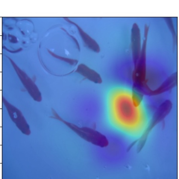
(b) Saliency map generated by Algorithm 1.

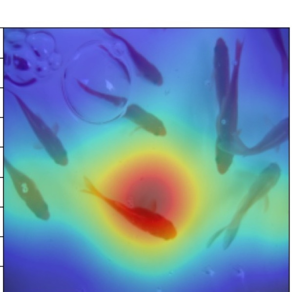
(c) Saliency map generated by Algorithm 2.

Figure 3: Example of an image with multiple salient regions.

Another reason of using a flipped mask in the saliency observations of Algorithm 2 is to handle images in which there are multiple salient parts. For example, the image of goldfish in Fig. 3(a) has multiple salient regions, namely, multiple goldfish. If we apply Algorithm 1, which does not use flipped masks, to this image, we obtain the saliency map in Fig. 3(b); obviously, the saliency map does not capture the salient parts in the image. This is because the value of $M(i,l)-M(i\odot m,l)$ in Line 7 of Algorithm 1 is almost same everywhere; this value becomes high for this image only if $m$ hides every goldfish in the image, which is difficult using only a single mask. Our method generates the saliency map in Fig. 3(c); an observed saliency value $M(i\odot\overline{{m}},l)-M(i\odot m,l)$ in Algorithm 2 is higher if $m$ hides at least one goldfish than if $m$ does not hide any goldfish.

Generating saliency map from resulting $\mu$. Algorithm 2 returns the saliency map $i_{\mathit{sal}}$ defined by $i_{\mathit{sal}}(\lambda)=\frac{1}{p}\sum_{i}\frac{1}{r_{i}^{2}}\mu(\lambda,r_{i})$. Instead of the saliency map computed by taking the simple average over every mask in Algorithm 1, the saliency map map returned by Algorithm 2 is the average weighted by the inverse of the area $\frac{1}{r_{i}^{2}}$ of each mask with the side size $r$. This weighted average gives more weight to the saliency values obtained by smaller masks. Using the weighted average helps a saliency map produced by Algorithm 2 localizes salient parts better than Algorithm 1.

3.2 Extension for Video-Classification Models

Algorithm 2 can be naturally extended for a video classifier with the following changes.

• The set of masks is extended, from 2D squares specified by their side length, to 3D rectangles specified by the side length of the square in a frame, and the number of frames that they hide. Suppose a mask $m$ with side length $r$ and the number of frames $t$ is applied to the pixel $\lambda$ at coordinate $(x,y)$ and at $n$-th frame of a video $i$. Then, $i\odot m$ is obtained by hiding the pixel at $(x,y)$ in each of the $n$-th to $(n+t-1)$-th frame with the 2D square mask specified by $r$.

• The type of functions drawn from the Gaussian process is changed to $f(\lambda,r,t)$ from $f(\lambda,r)$ in Algorithm 2 reflecting the change of the definition of masks.

• The algorithm takes $T:=\{{t_{1},\dots,t_{k}}\}$ in addition to $L$; the set $T$ expresses the allowed variation of parameter $t$ of a mask.

• The expression to update $i_{\mathit{sal}}$ in Line 12 of Algorithm 2 is changed to $\frac{1}{pk}\sum_{i}\sum_{s}\frac{1}{r_{i}^{2}t_{s}}\mu(\lambda,r_{i},t_{s})$; the weight is changed to the reciprocal of the volume of each mask.

4 Experiments

We implemented Algorithm 2 and conducted experiments to evaluate the effectiveness of BOREx.Due to the limited space, we report a part of the experimental results. See the appendix for the experimental environment and more results and discussions, particularly on video classification.

The research questions that we are addressing are the following.

RQ1:

Does BOREx improve the quality of an input saliency map? This is to evaluate that BOREx is useful to refine a potentially low-quality saliency map, which is the main claim of this paper.

RQ2:

Does Algorithm 2 produce a better saliency map than one produced by Algorithm 1 by Mokuwe et al. [16]? This is to demonstrate the merit of BOREx over the algorithm by Mokuwe et al.

RQ3:

Does the extension in Section 3.2 useful as a saliency-map generation for video classifiers? This is to evaluate the competency of BOREx to explain a video-classification result.

Evaluation metrics.

To quantitatively evaluate the quality of a saliency map, we used the following three measures.

Insertion:

For a saliency map $i_{\mathit{sal}}$ explaining a classification of an image $i$ to label $l$, the insertion metric is defined as $\sum_{k}M(i^{(k)},l)$, where $i^{(k)}$ is the image obtained by masking all the pixels other than those with top-$k$ saliency values in $i_{\mathit{sal}}$ to black.

Deletion:

The deletion metric is defined as $\sum_{k}M(i^{(-k)},l)$, where $i^{(-k)}$ is the image obtained by masking all the pixels with top-$k$ saliency values in $i_{\mathit{sal}}$ to black.

F-measure:

The F-measure in our experiments is defined as $\sum_{k}F(i^{(k)},l,B_{i,l})$, where $F(i^{(k)},l,B_{i,l})$ is the F-measure calculated from the recall and the precision of the pixels in $i^{(k)}$ against the human-annotated bounded region $B_{i,l}$ in $i$ that indicates an object of label $l$.

The insertion and the deletion metrics are introduced by [17] to quantitatively evaluate how well a saliency map localizes a region that is important for a decision by a model. The higher value of the insertion metric is better; the lower value of the deletion metric is better. The higher insertion implies that $i_{\mathit{sal}}$ localizes regions in $i$ that are enough for classifying $i$ to $l$. The lower deletion implies that $i_{\mathit{sal}}$ localizes regions that are indispensable for classifying $i$ to $l$. The F-measure is an extension of their pointing-game metric also to consider recall, not only the precision. The higher value of F-measure is better, implying $i_{\mathit{sal}}$ points out more of an important region correctly.

In what follows, we use a statistical hypothesis test called the one-sided Wilcoxon signed-rank test [26] (or, simply Wilcoxon test). This test is applied to matched pairs of values $\{(a_{1},b_{1}),\dots,(a_{n},b_{n})\}$ sampled from a distribution and can be used to check whether the median of $\{a_{1},\dots,a_{n}\}$ can be said to be larger or smaller than that of $\{b_{1},\dots,b_{n}\}$ with significance. To compare saliency generation methods $X$ and $Y$, we calculate the pairs of the values of metrics evaluated with a certain dataset, the first of each are of the method $X$ and the second are of $Y$; then, we apply the Wilcoxon test to check the difference in the metrics. For further details, see [26].

To address these RQs, we conducted the following experiments:

RQ1:

We used RISE [17] and Grad-CAM++ [5] to generate saliency maps for the images in PascalVOC dataset [8]; we write $D_{\mathrm{RISE}}$ and $D_{\mathrm{GradCAM++}}$ for the set of saliency maps generated by RISE and Grad-CAM++, respectively. Then, we applied BOREx with these saliency maps as input; we write $D_{\mathrm{RISE}}^{\mathrm{BOREx}}$ (resp., $D_{\mathrm{GradCAM++}}^{\mathrm{BOREx}}$) for the saliency maps generated using $D_{\mathrm{RISE}}$ (resp., $D_{\mathrm{GradCAM++}}$) as input. We check whether the quality of the saliency maps in $D_{-}^{\mathrm{BOREx}}$ is better than $D_{-}$ by the one-sided Wilcoxon signed-rank test. If so, we can conclude that BOREx indeed improves the saliency map generated by other methods.

RQ2:

We generated saliency maps for the PascalVOC dataset using Mokuwe et al. [16] presented in Algorithm 1; we write $D_{\mathrm{BO}}$ for the generated saliency maps. We check if the quality of the saliency maps in $D_{\mathrm{RISE}}^{\mathrm{BOREx}}$ is better than $D_{\mathrm{BO}}$ by one-sided Wilcoxon signed-rank test. If so, we can conclude the merit of BOREx over the method by Mokuwe et al.

RQ3:

We generated saliency maps for the dataset in Kinetics-400 using an extension of GradCAM++ and RISE for video classification implemented by us; let the set of saliency maps $D_{M,\mathrm{GradCAM++}}$ and $D_{M,\mathrm{RISE}}$, respectively. Then, we applied BOREx with these saliency maps as input; we write $D_{\mathrm{M,RISE}}^{\mathrm{BOREx}}$ (resp., $D_{\mathrm{M,GradCAM++}}^{\mathrm{BOREx}}$) for the saliency maps generated using $D_{\mathrm{M,RISE}}$ (resp., $D_{\mathrm{M,GradCAM++}}$) as input. We check whether the quality of the saliency maps in $D_{M,-}^{\mathrm{BOREx}}$ is better than $D_{M,-}$ by one-sided Wilcoxon signed-rank test. If so, we can conclude the merit of BOREx as an explanation method for a video-classification result.

As the model whose classification behavior to be explained, we used ResNet-152 [11] obtained from torchvision.models, which is pre-trained with ImageNet [6], for RQ1 and RQ2; and i3D [4] obtained from TensorFlow Hub, which is pre-trained with Kinetics-400 [13]. Notice that the datasets PascalVOC and Kinetics-400 provide human-annotated bounding regions for each label and each image, enabling computation of the F-measure.

4.1 Results and Discussion

(a) Input

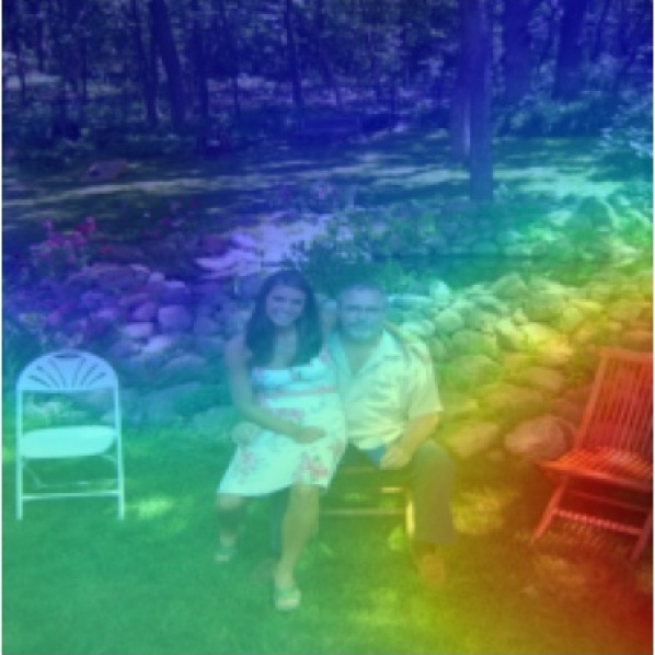
(b) BOREx

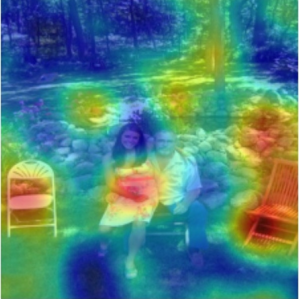
(c) RISE

Figure 4: Image of chairs and saliency maps to explain it.

RQ1.

Table 1 shows that BOREx improved the quality of the saliency maps generated by RISE and Grad-CAM++ in several metrics with statistical significance ($p<0.001$). Therefore, we conclude that BOREx successfully refines an input saliency map. This improvement is thanks to the Gaussian process regression that successfully captured the locality of the salient pixels. For example, the saliency maps in Fig. 1 suggest that BOREx is better at generalizing the salient pixels to the surrounding areas than RISE.

The time spent for GPR-based optimization was $9.26\pm 0.26$ seconds in average for each image. We believe this computation time pays off if we selectively apply BOREx to saliency maps whose quality needs to be improved.

To investigate the effect of the features of BOREx presented in Section 3.1 (i.e., flipped masks and the saliency-map computation from the result of GPR by weighted average in its performance), we conducted an ablation study; the result is shown in Table 2. We compared BOREx with (1) a variant that does not use flipped masks (no-flip), (2) a variant that uses simple average instead of the average weighted by the inverse of the area of masks (simple-avg), and (3) a variant that does not use prior (no-prior). The statistical test demonstrates that flipped masks and weighted averages are effective in the performance of BOREx. However, the effectiveness over the no-prior variant is not confirmed. This is mainly because, if the quality of a given prior is already high, the effectiveness of BOREx is limited. Indeed, BOREx is confirmed to be effective over the no-prior case if the insertion metric of the priors is less than 0.6; see the row “no-prior (base insertion $<0.6$)” in Table 2.

The statistical test did not demonstrate the improvement in the deletion metric for a saliency map generated by RISE and the F-measure for a saliency map generated by Grad-CAM++. Investigation of several images for which BOREx degrades the metrics reveals that this is partly because the current BOREx allows only square-shaped masks; this limitation degrades the deletion metric for an image with multiple objects with the target label $l$. For example, a single square-shaped mask cannot focus on both chairs simultaneously in the image in Fig. 4(a). For such an image, BOREx often focuses on only one of the objects, generating the saliency map in Fig. 4(b). Even if we mask the right chair in Fig. 4(a), we still have the left chair, and the confidence of the label “chair” does not significantly decrease, which degrades the deletion metric of the BOREx-generated saliency map.

Table 1: Result of the experiments. “Image/Video”: The kind of the classifier; “Compared with”: the baseline method; “Metric”: evaluation metric; “$p$-value”: the $p$-value. The null hypothesis of each test expresses that the average of the metric of BOREx is not better than that of baseline. One asterisk indicates $p<0.05$; two asterisks indicates $p<0.001$.

Image/Video	Compared with	Metric	$p$-value
Image	RISE	F-measure	8.307e-21∗∗
		insertion	1.016e-23∗∗
		deletion	8.874e-01
	Grad-CAM++	F-measure	1.000
		insertion	5.090e-08∗∗
		deletion	6.790e-04∗∗
	BO	F-measure	1.800e-05∗∗
		insertion	6.630e-11∗∗
		deletion	3.111e-01
Video	RISE	F-measure	4.988e-07∗∗
		insertion	8.974e-01
		deletion	8.161e-18∗∗
	Grad-CAM++	F-measure	9.9980e-01
		insertion	3.636e-01
		deletion	2.983e-07∗∗

RQ2.

The last three rows of Table 1 show that the use of an initial saliency map improved the quality of the saliency maps generated by Bayesian optimization in terms of several metrics with statistical significance compared to the case where the initial saliency map is not given ($p<0.001$). Therefore, we conclude that BOREx produces a better saliency map than the one produced by Mokuwe et al. in terms of the insertion metric and F-measure.

The improvement was not concluded in terms of the deletion metrics. Investigation of the generated saliency maps suggests that such degradation is observed when the quality of a given initial saliency map is too low; if such a saliency map is given, it misleads an execution of BOREx, which returns a premature saliency map at the end of the prespecified number of iterations.

Table 2: The result of ablation study.

Compared with	Metric	$p$-value
no-flip	F-measure	2.987e-29∗∗
	insertion	1.416e-04∗∗
	deletion	2.024e-03∗
simple-avg	F-measure	2.026e-03∗
	insertion	1.184e-46∗∗
	deletion	4.871e-03∗
no-prior	F-measure	4.514e-02∗
	insertion	3.84624e-01
	deletion	2.2194e-01
no-prior (base insertion $<0.6$)	F-measure	2.4825e-02∗
	insertion	3.219e-03∗
	deletion	6.47929e-01

RQ3.

Table 1 shows the result of the experiment for RQ3. It shows that the saliency maps generated by the extensions of RISE and Grad-CAM++ for video classifiers are successfully refined by BOREx in terms of at least one metric with statistical significance ($p<0.001$). Therefore, we conclude that a saliency map produced by BOREx points out regions in a video that are indispensable to explain the classification result better than the other methods.

The improvement in the insertion metric over RISE and Grad-CAM++, and in F-measure over Grad-CAM++ were not concluded. The investigation of saliency maps whose quality is degraded by BOREx reveals that the issue is essentially the same as that of the images with multiple objects discussed above. A mask used by BOREx occludes the same position across several frames; therefore, for a video in which an object with the target label moves around, it is difficult to occlude all occurrences of the object in different frames. This limitation leads to a saliency map generated by BOREx that tends to point out salient regions only in a part of the frames, which causes the degradation in the insertion metric. The improvement in deletion metric seems to be due to the mask shape of BOREx. To improve the deletion metric for a video-classifier explanation, a saliency map must point out a salient region across several frames. The current mask shape of BOREx is advantageous, at least for a video in which there is a single salient object that does not move around, to cover the salient object over several frames.

5 Conclusion

This paper has presented BOREx, a method to refine a potentially low-quality saliency map that explains a classification result of image and video classifiers. Our refinement of a saliency map with Bayesian optimization applies to any existing saliency-map generation method. The experiment results demonstrate that BOREx improves the quality of the saliency maps, especially when the quality of the given saliency map is neither too high nor too low.

We are currently looking at enhancing BOREx by investigating the optimal shape of masks to improve performance. Another important research task is making BOREx more robust to an input saliency map with very low quality.

Appendix 0.A The detail of experimental environment

We implemented Algorithm 2using Python 3.6.12 and PyTorch 1.6.0. The experiments on image classification are conducted on a GPU workstation with 3.60 GHz Intel Core i7-6850K, 12 CPUs, NVIDIA Quadro P6000, and 32GB RAM that runs Ubuntu 20.04.2 LTS (64 bit) and CUDA 11.0. The experiments on video classification are conducted on a GPU workstation with 3.00 GHz Intel Xeon E5-2623 v3, 16 CPUs, NVIDIA Tesla P100, and 500GB RAM that runs Ubuntu 16.04.3 LTS (64 bit). In the implementation of Algorithm 2, we used Matérn kernel defined as follows:

$$k((\lambda_{1},r_{1}),(\lambda_{2},r_{2})):=\frac{2^{1-\nu}}{\Gamma(\nu)}{\left(\frac{\sqrt{2\nu}d^{\prime}}{l}\right)}^{\nu}K_{\nu}\left({\frac{\sqrt{2\nu}d^{\prime}}{l}}\right),$$

where $d^{\prime}$ is the Euclidean distance between $(\lambda_{1},r_{1})$ and $(\lambda_{2},r_{2})$ (i.e., $\sqrt{d(\lambda_{1},\lambda_{2})^{2}+(r_{1}-r_{2})^{2}}$ where $d(\lambda_{1},\lambda_{2})$ is the Euclidean distance between $\lambda_{1}$ and $\lambda_{2}$ in the input image); $\nu$ and $l$ are positive parameters that control the shape of the function; $\Gamma$ is the gamma function; and $K_{\nu}$ is a modified Bessel function [AbraSteg72]. Mokuwe et al. [16] used $\nu=2.5$ and $l=12$ in their implementation. We use the Matérn kernel with $\nu=1.5$ and $l=12$.

Appendix 0.B Results of additional experiments

Table 3: Comparison of the results produced by different number of $N$ in Algorithm 2. Each result uses an input saliency map generated by RISE with $100$ masks. “BO$n$” represents Algorithm 2with $N=n$. Each column represents the following: “Metric” for the metric; “Base.” for the baseline; “Comp.” for the compared method; “$p$-val.” for the $p$-value. One asterisk indicates $p<0.05$; two asterisks indicates $p<0.001$.

Metric	Base.	Comp.	$p$-val.
Insertion	BO10	BO50	7.042e-36∗∗
	BO10	BO80	4.023e-38∗∗
	BO10	BO100	2.261e-38∗∗
	BO50	BO80	8.156e-02
	BO50	BO100	7.542e-02
	BO80	BO100	3.066e-01
Deletion	BO10	BO50	2.937e-32∗∗
	BO10	BO80	1.838e-38∗∗
	BO10	BO100	2.007e-41∗∗
	BO50	BO80	4.454e-03∗
	BO50	BO100	1.132e-04∗∗
	BO80	BO100	3.721e-02∗
F-measure	BO10	BO50	4.825e-32∗∗
	BO10	BO80	1.442e-34∗∗
	BO10	BO100	1.010e-34∗∗
	BO50	BO80	1.606e-03∗
	BO50	BO100	7.387e-04∗∗
	BO80	BO100	5.806e-01

Table 4: Two-sided test to compare the results produced by different number of $N$ in Algorithm 2. Each result uses an input saliency map generated by RISE with $100$ masks.

Metric	Base.	Comp.	$p$-val.
Insertion	BO10	BO50	1.408e-35∗∗
	BO10	BO80	8.046e-38∗∗
	BO10	BO100	4.522e-38∗∗
	BO50	BO80	1.631e-01
	BO50	BO100	1.508e-01
	BO80	BO100	6.131e-01
Deletion	BO10	BO50	5.875e-32∗∗
	BO10	BO80	3.677e-38∗∗
	BO10	BO100	4.013e-41∗∗
	BO50	BO80	8.907e-03∗
	BO50	BO100	2.264e-04∗∗
	BO80	BO100	7.442e-02
F-measure	BO10	BO50	9.650e-32∗∗
	BO10	BO80	2.884e-34∗∗
	BO10	BO100	2.020e-34∗∗
	BO50	BO80	3.212e-03∗
	BO50	BO100	1.477e-03∗
	BO80	BO100	8.388e-01

Table 5: Comparison of the results of Algorithm 2with input saliency maps produced by RISE with different number of masks. $N$ is set to $50$ in each execution of Algorithm 2. “RISE$n$” represents input salinecy maps produced by RISE with $n$ masks are used. Each column represents the following: “Metric” for the metric; “Base.” for the baseline; “Comp.” for the compared method; “$p$-val.” for the $p$-value. One asterisk indicates $p<0.05$; two asterisks indicates $p<0.001$.

Metric	Base.	Comp.	$p$-val.
Deletion	RISE0	RISE100	8.453e-01
	RISE0	RISE300	6.630e-01
	RISE0	RISE500	6.202e-01
	RISE0	RISE1000	3.491e-01
	RISE100	RISE300	3.976e-01
	RISE100	RISE500	3.277e-01
	RISE100	RISE1000	1.773e-01
	RISE300	RISE500	4.381e-01
	RISE300	RISE1000	2.786e-01
	RISE500	RISE1000	2.085e-01
F-meas.	RISE0	RISE100	1.123e-01
	RISE0	RISE300	1.131e-02∗
	RISE0	RISE500	1.81777e-01
	RISE0	RISE1000	1.636e-01
	RISE100	RISE300	4.176e-01
	RISE100	RISE500	7.307e-01
	RISE100	RISE1000	5.568e-01
	RISE300	RISE500	7.514e-01
	RISE300	RISE1000	9.475e-01
	RISE500	RISE1000	3.592e-01
Insertion	RISE0	RISE100	4.525e-02
	RISE0	RISE300	3.566e-03∗
	RISE0	RISE500	3.518e-03∗
	RISE0	RISE1000	1.101e-03∗
	RISE100	RISE300	2.698e-01
	RISE100	RISE500	1.473e-01
	RISE100	RISE1000	7.709e-02
	RISE300	RISE500	3.091e-01
	RISE300	RISE1000	1.492e-01
	RISE500	RISE1000	2.151e-01

Table 6: Two-sided test to compare Algorithm 2with input saliency maps produced by RISE with different number of masks.

Metric	Base.	Comp.	$p$-val.
Deletion	RISE0	RISE100	3.09308e-01
	RISE0	RISE300	6.73922e-01
	RISE0	RISE500	7.59515e-01
	RISE0	RISE1000	6.98164e-01
	RISE100	RISE300	7.95128e-01
	RISE100	RISE500	6.55416e-01
	RISE100	RISE1000	3.54525e-01
	RISE300	RISE500	8.76144e-01
	RISE300	RISE1000	5.57116e-01
	RISE500	RISE1000	4.17039e-01
F-meas.	RISE0	RISE100	2.24636e-01
	RISE0	RISE300	2.2610e-02∗
	RISE0	RISE500	3.63555e-01
	RISE0	RISE1000	3.27184e-01
	RISE100	RISE300	8.35268e-01
	RISE100	RISE500	5.38648e-01
	RISE100	RISE1000	8.86484e-01
	RISE300	RISE500	4.97256e-01
	RISE300	RISE1000	1.04953e-01
	RISE500	RISE1000	7.18478e-01
Insertion	RISE0	RISE100	4.5251e-02∗
	RISE0	RISE300	3.566e-03∗
	RISE0	RISE500	3.518e-03∗
	RISE0	RISE1000	1.101e-03∗
	RISE100	RISE300	2.698e-01
	RISE100	RISE500	1.473e-01
	RISE100	RISE1000	7.709e-02
	RISE300	RISE500	3.091e-01
	RISE300	RISE1000	1.492e-01
	RISE500	RISE1000	2.151e-01

0.B.1 Effect of increasing $N$ in Algorithm 2

We executed Algorithm 2with different $N$, the number of iterations for Gaussian process regression. With more iterations, the estimated $\mu$ is expected to be more precise. However, the time spent in one iteration in the later iterations tends to be longer because there are more observations to fit.

Tables 3 and 4 show the result. We observe the significant improvement in the insertion metric only when we increased $N$ from 10 to the other values; in the other cases, improvement nor degradation is not concluded (Table 4). For the other metrics, increasing $N$ from 50 to the other values is also concluded to be effective. In any metrics, increasing $N$ from 80 to 100 was not concluded to be effective. This result suggests that increasing $N$, which incurs time for executing Algorithm 3, is effective; however, the merit of increasing the number beyond certain number (here 50) is limited.

0.B.2 Effect of the quality of an input saliency map on the output of Algorithm 2

We executed Algorithm 2with input maps generated by RISE with different numbers of masks. This experiment is to study the effect of the quality of an input saliency map on the output because the quality of an input saliency map is expected to be higher with more masks.

Table 5 shows the result. Significant improvement is observed (1) in the insertion metric when we increased the number of masks from 0 to 300 or more and (2) in the F-measure when we increased the number of masks from 0 to 300. We cannot conclude the significant improvement in the other cases. The two-sided test we conducted, whose result is presented in Table 6, does not conclude that the quality of the saliency maps measured in these metrics differ among the input saliency maps generated by RISE with different numbers of masks, which implies that the quality is not degraded by increasing the number of masks. These results back our conclusion of BOREx is effective to improve a low-quality saliency map in terms of the insertion metric.

Appendix 0.C Examples of saliency maps

0.C.1 Examples in which BOREx successfully improves input images

(a) Input

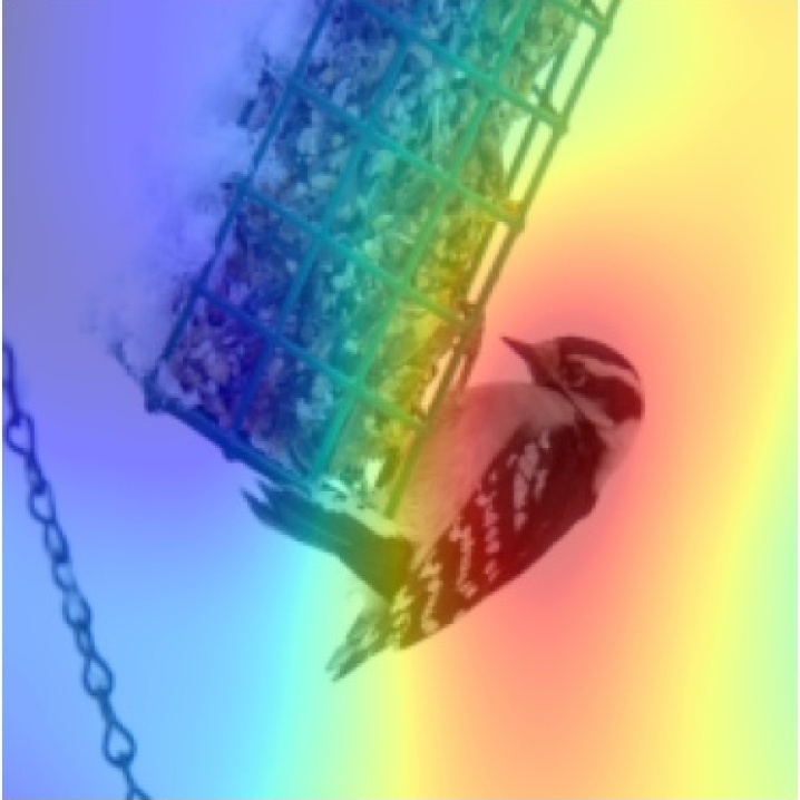
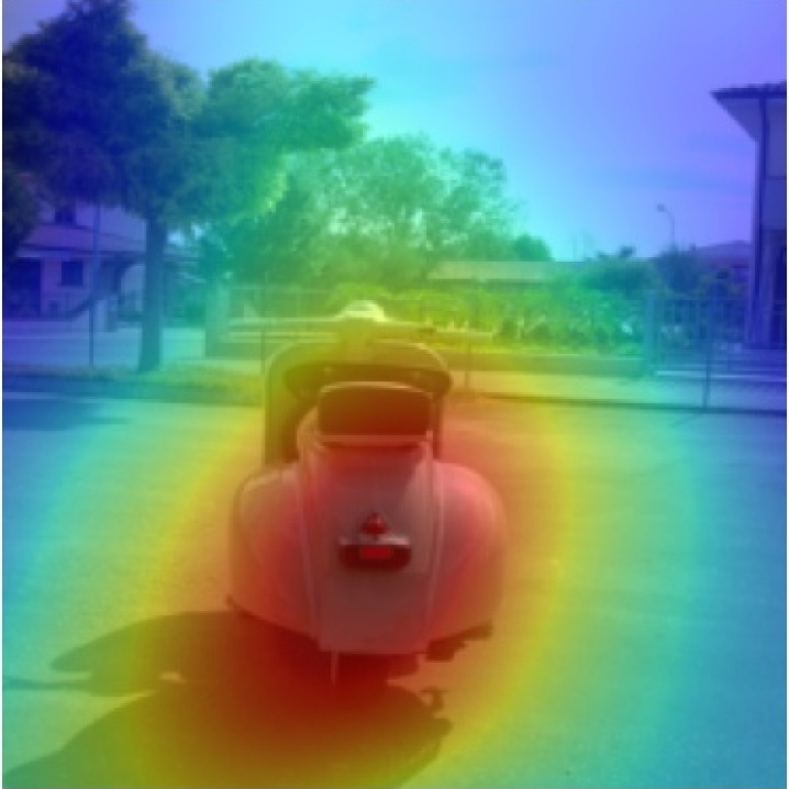
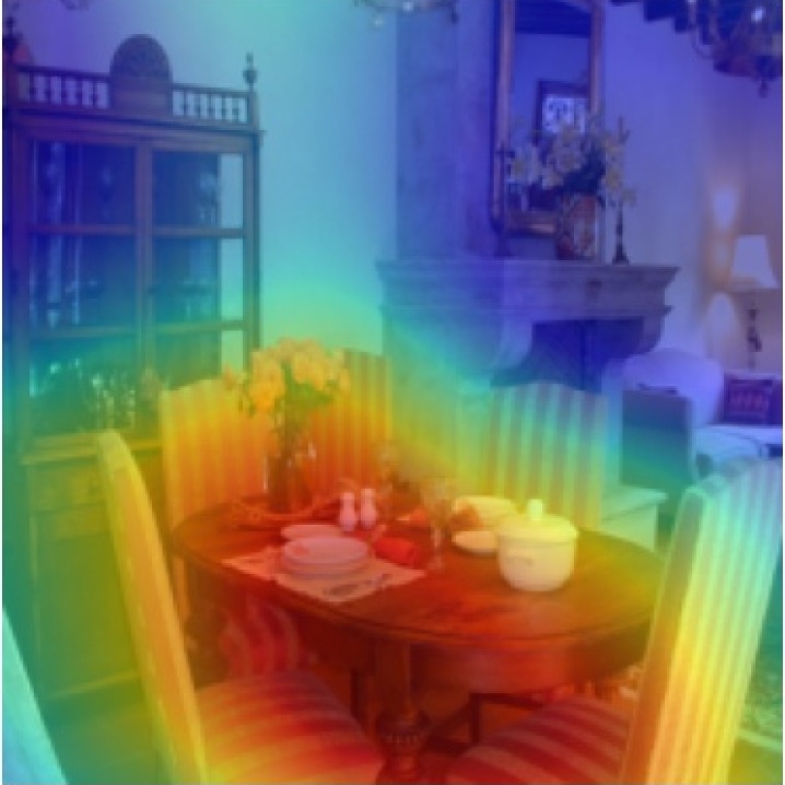
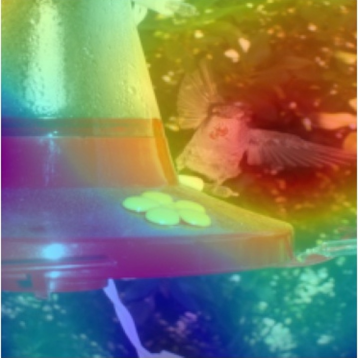
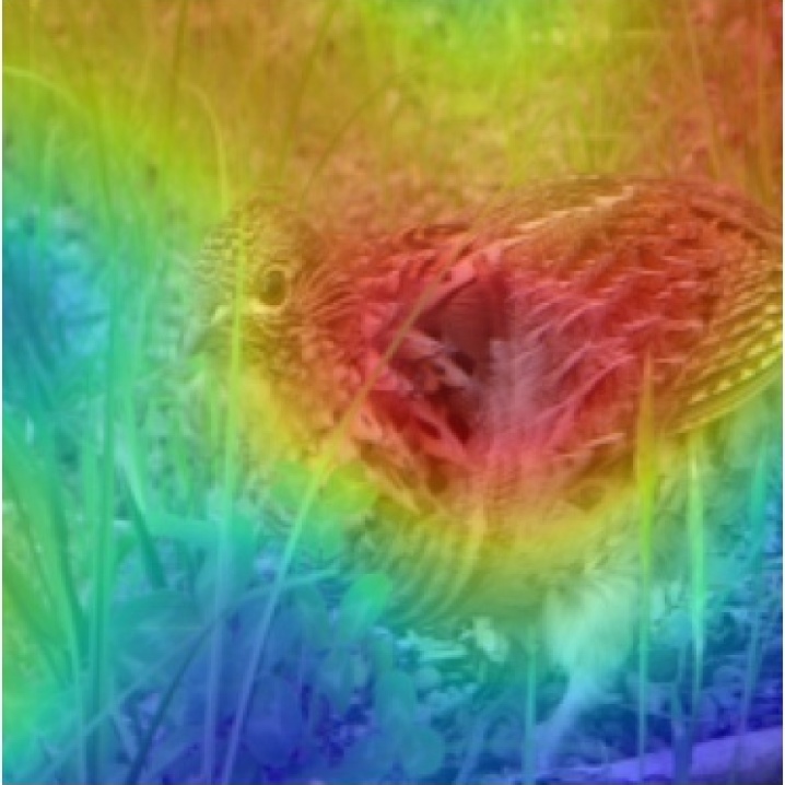
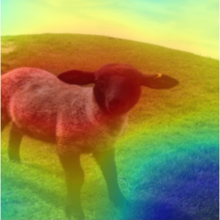
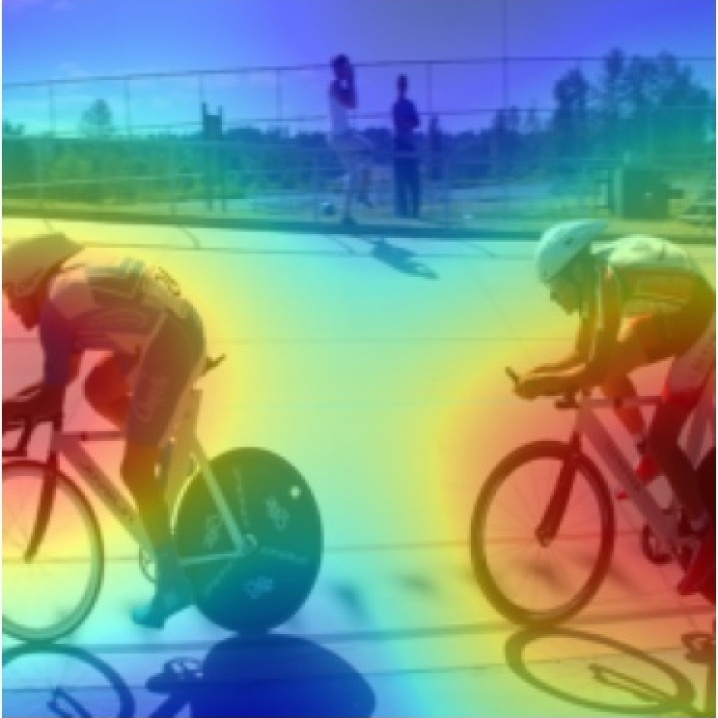
(b) BOREx

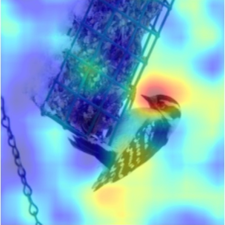
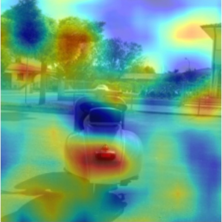
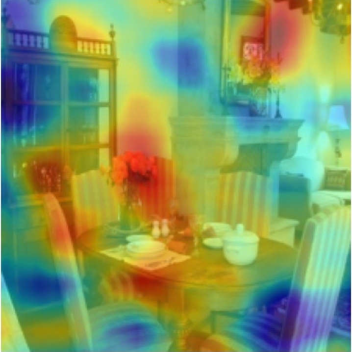
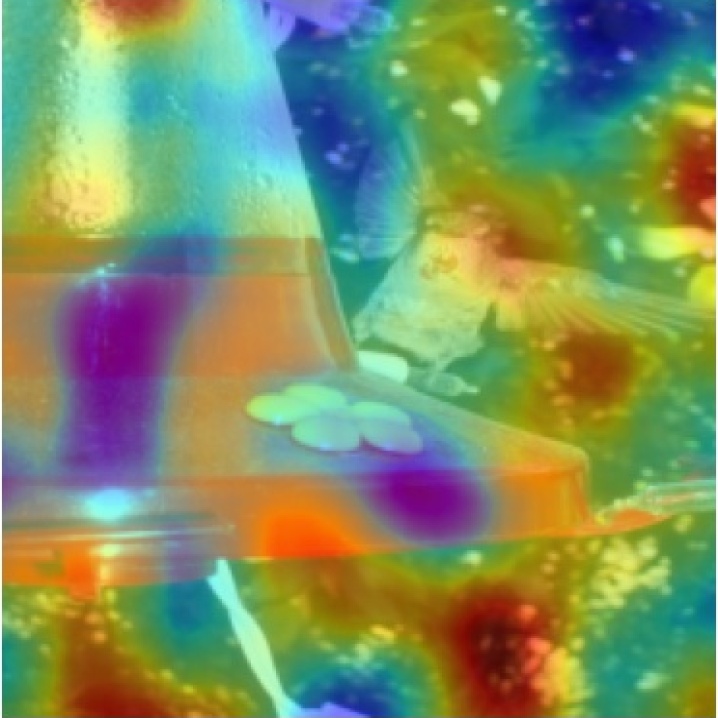
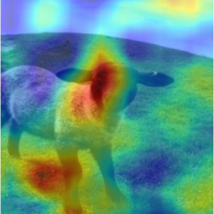
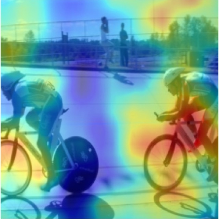
(c) RISE

Figure 5: Examples of saliency maps that are successfully refined by BOREx. The labels used in each explanation are: “bird”, “motor bike”, “dining table”, “bird”, “bird”, “sheep”, and “bicycle”, from the first row.

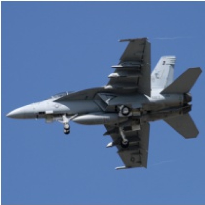
(a) Input

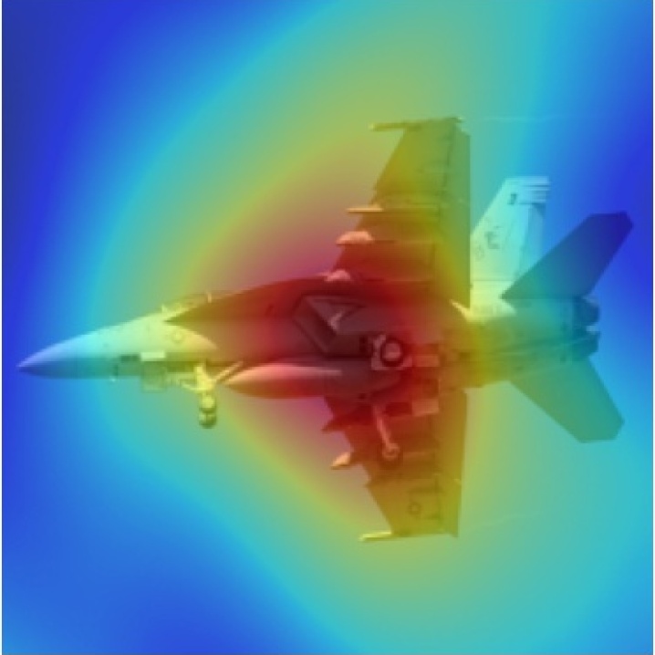
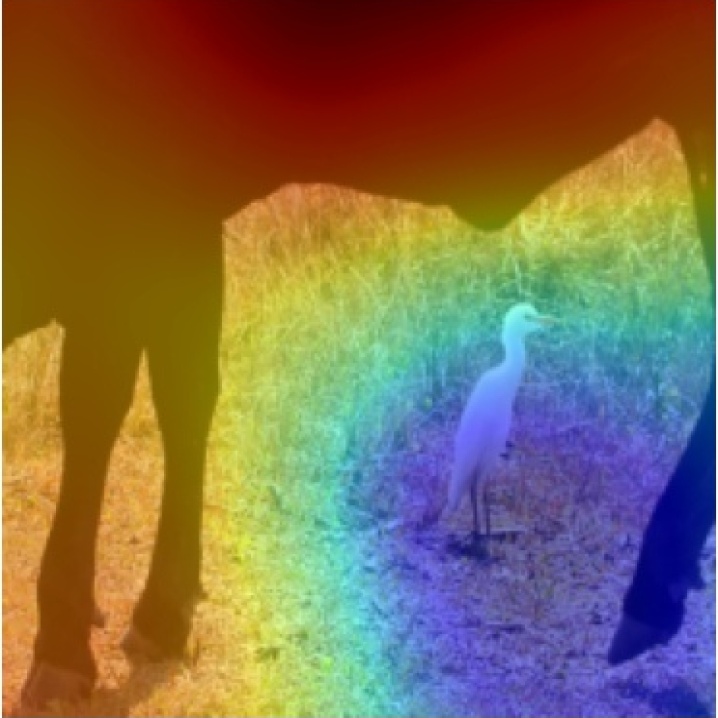
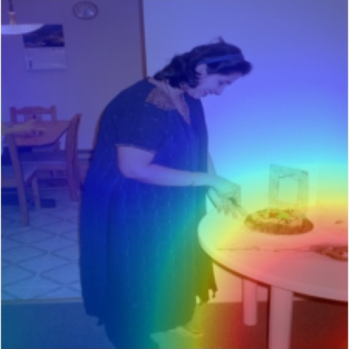
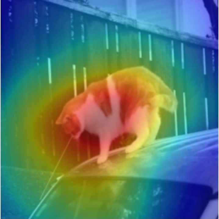
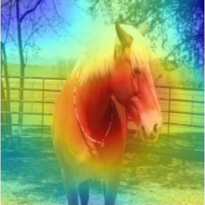
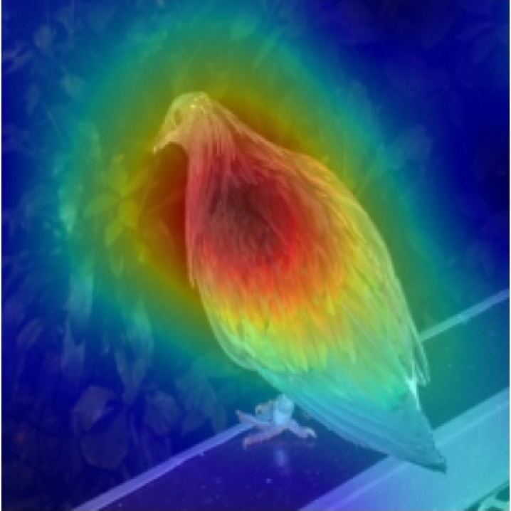
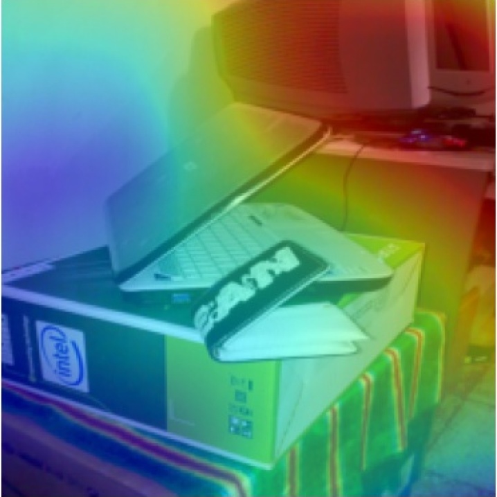
(b) BOREx

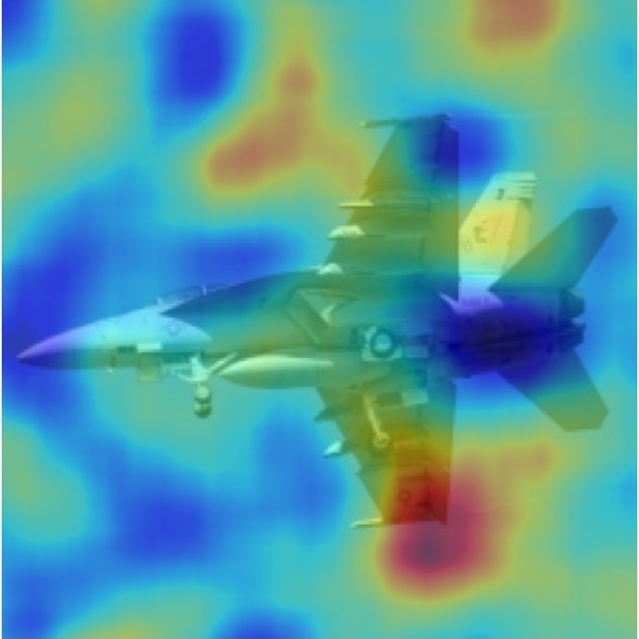
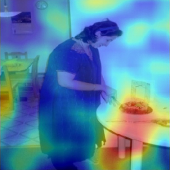
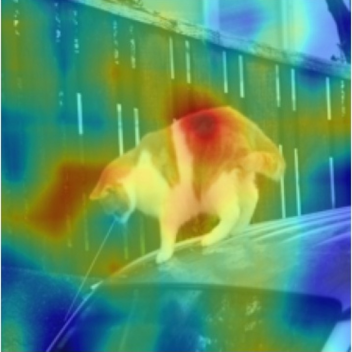
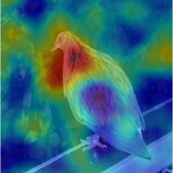
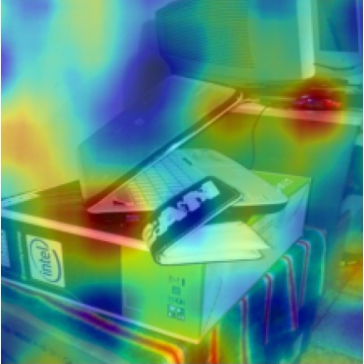
(c) RISE

Figure 6: Examples of saliency maps that are successfully refined by BOREx. The labels used in each explanation are: “aeroplane”, “cow”, “dining table”, “cat”, “horse”, “bird”, and “TV monitor”, from the first row.

(a) Input

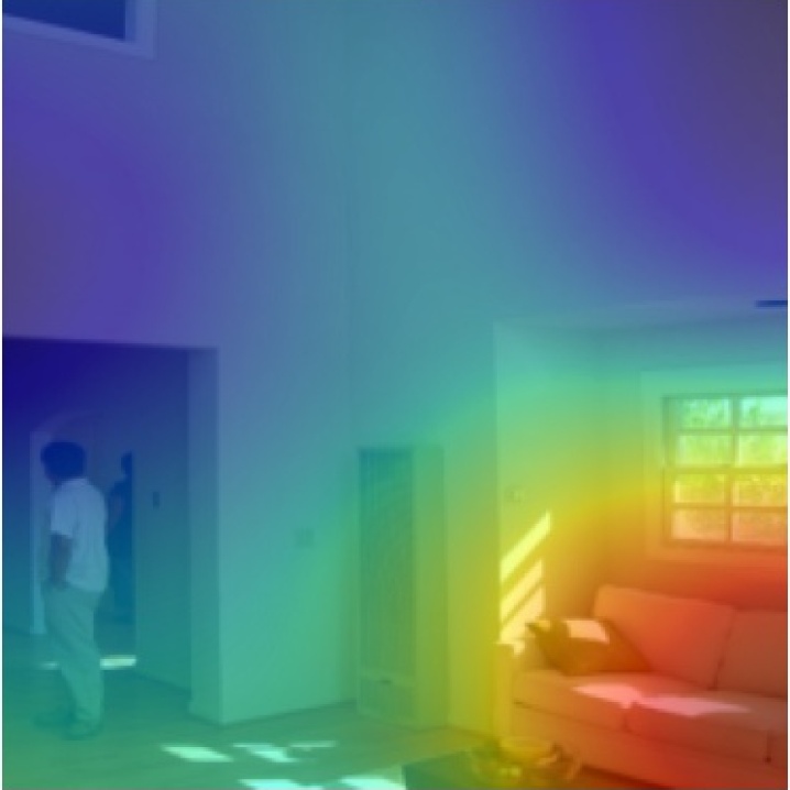
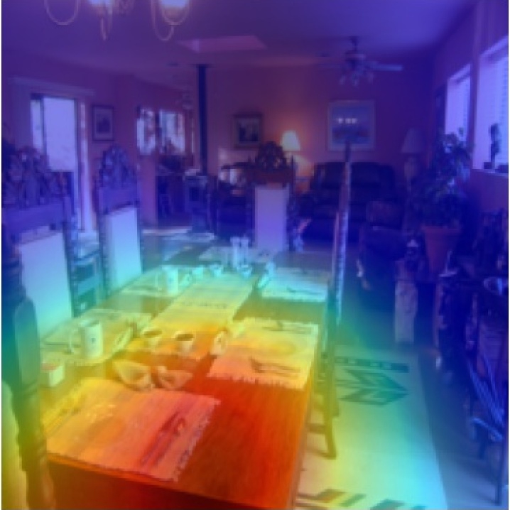
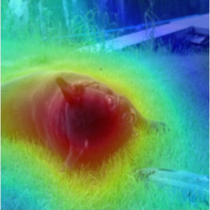
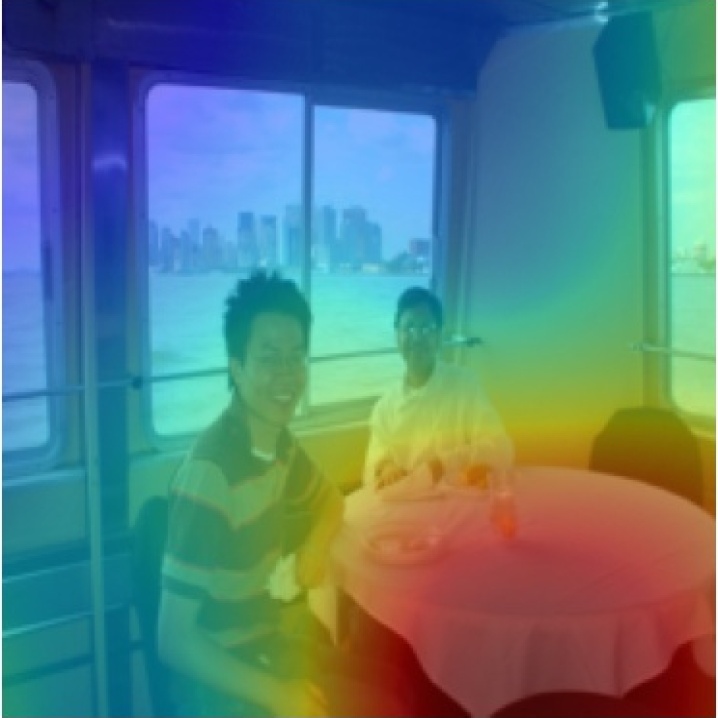
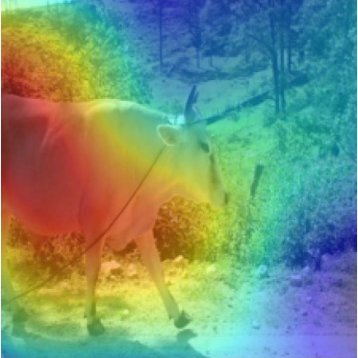
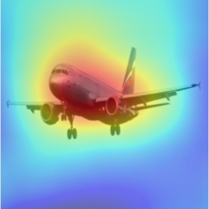
(b) BOREx

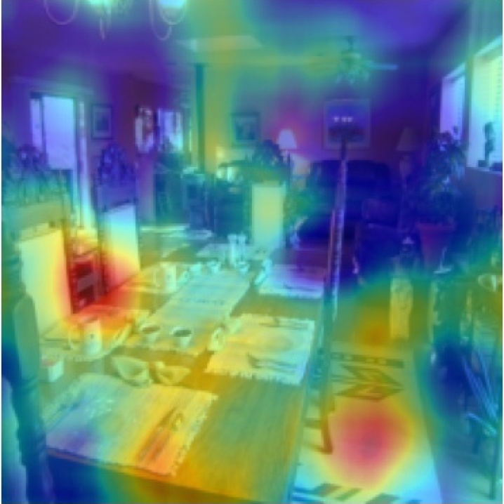
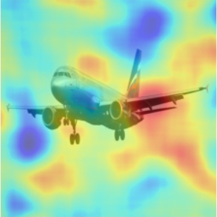
(c) RISE

Figure 7: Examples of saliency maps that are successfully refined by BOREx. The labels used in each explanation are: “sofa”, “car”, “dining table”, “dog”, “dining table”, “cow”, and “aero plane”, from the first row.

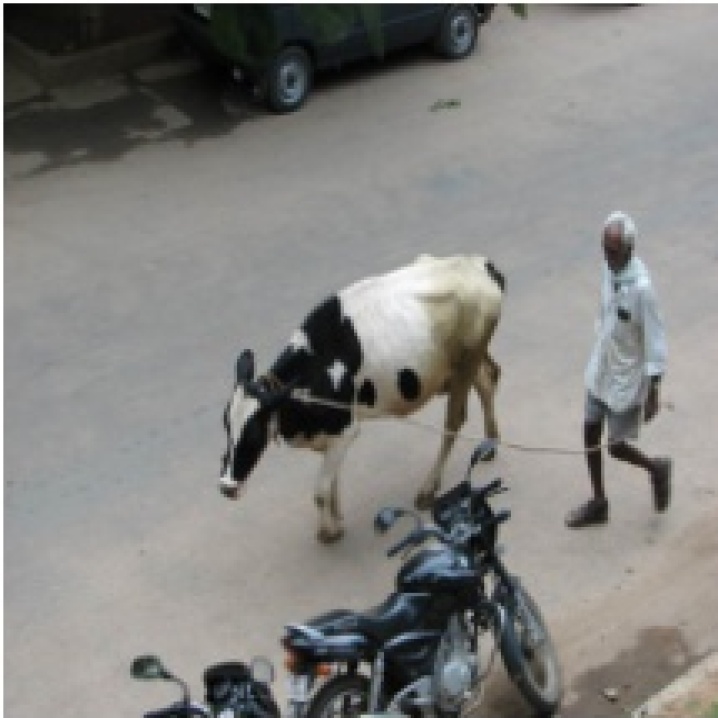
(a) Input

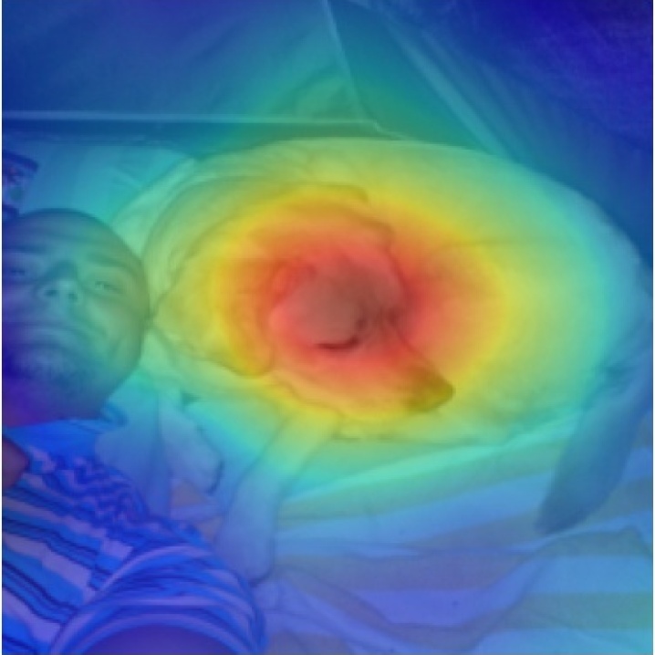
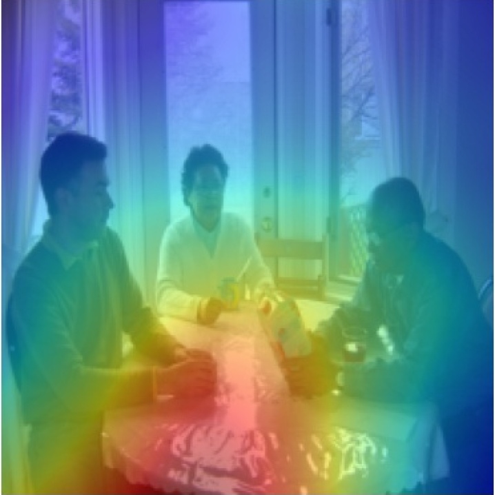
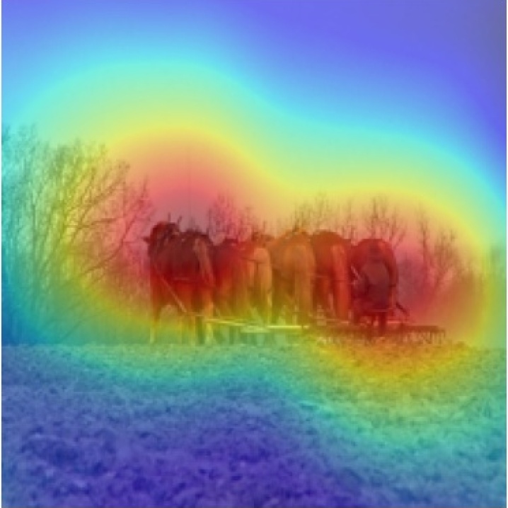
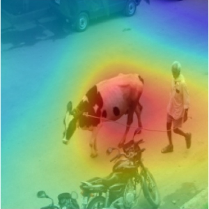
(b) BOREx

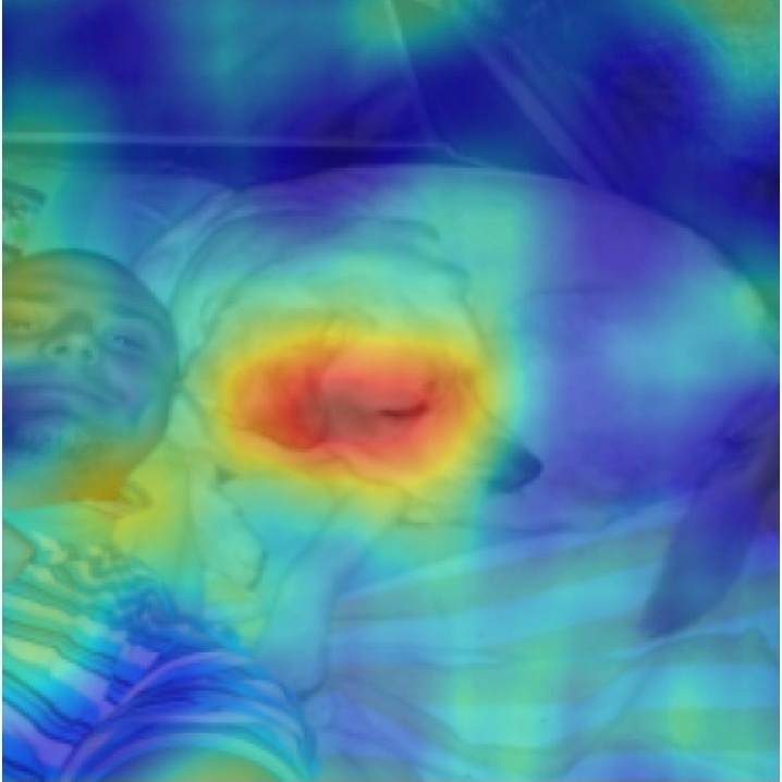
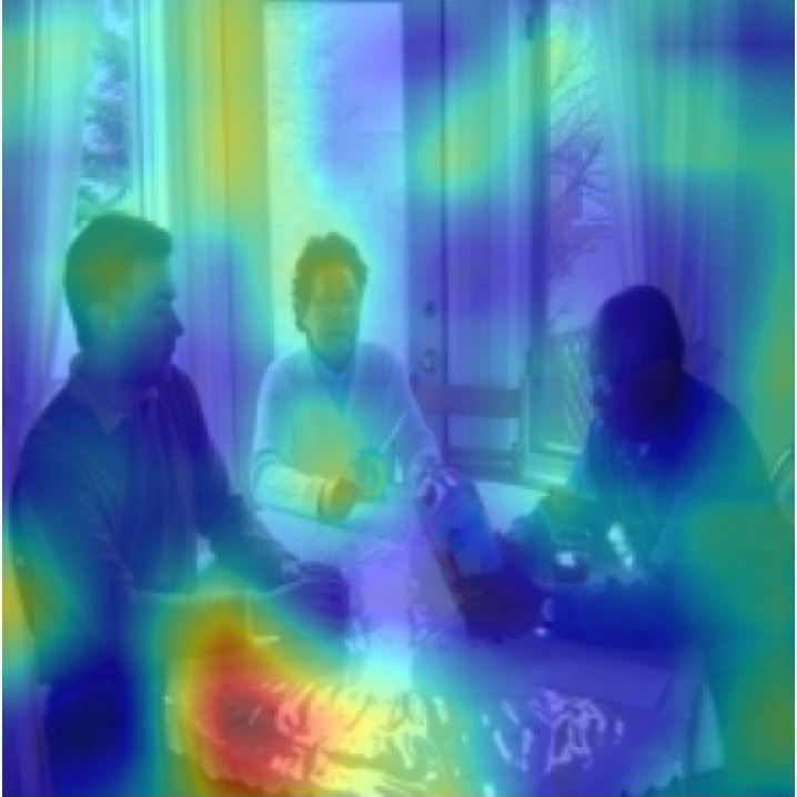
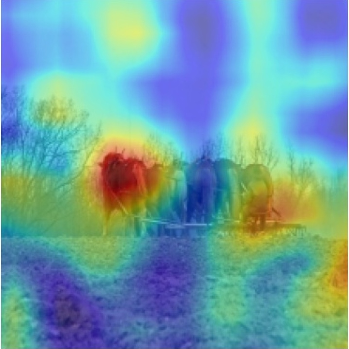
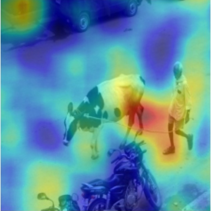
(c) RISE

Figure 8: Examples of saliency maps that are successfully refined by BOREx. The labels used in each explanation are: “dog”, “dining table”, “horse”, “bird”, and “cow”, from the first row.

Figures 5–8 present examples of saliency maps generated by BOREx. We picked several examples in which BOREx successfully refines the quality of input images measured in the quantitative metrics. Compared to the input images generated by RISE, the saliency maps generated by BOREx localize the important regions better and less noisy.

0.C.2 Examples in which BOREx degraded the quality of input images

Figure 9 presents the examples in which BOREx degraded the input images measured in the quantitative metrics. We add explanations for each example.

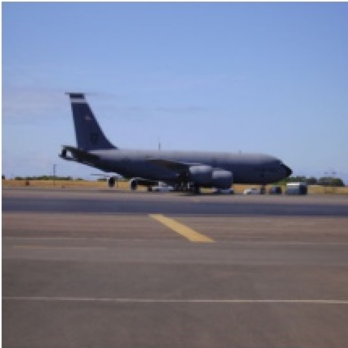
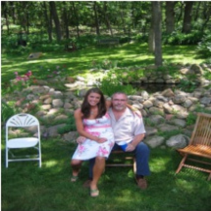
(a) Input

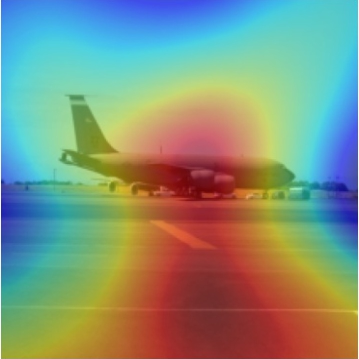
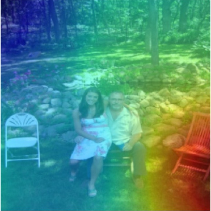
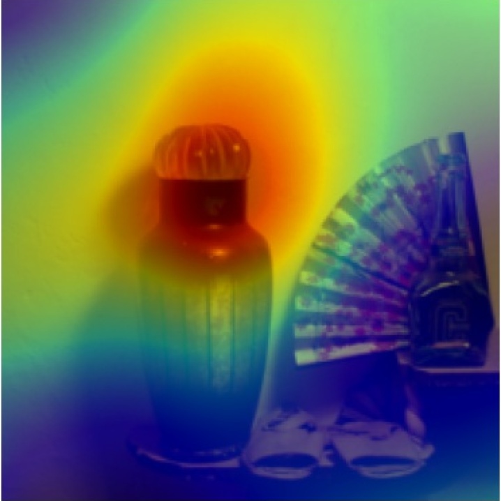
(b) BOREx

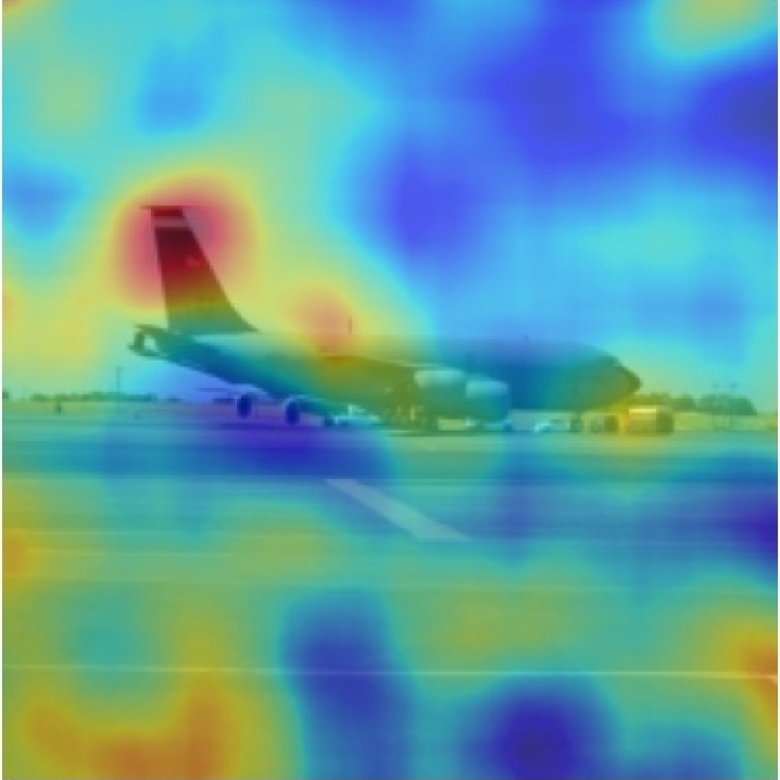
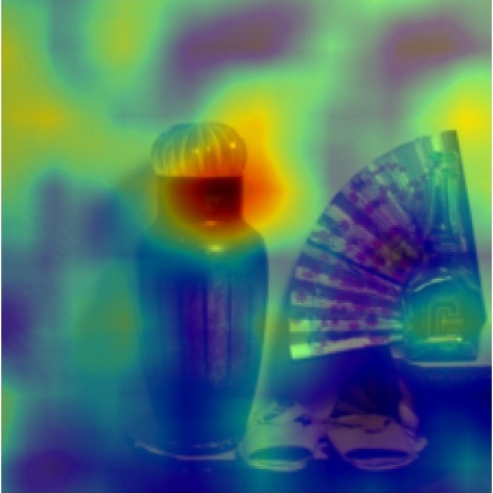
(c) RISE

Figure 9: Examples of saliency maps that BOREx degraded the quantitative metric of the input image synthesized by RISE. The labels used in each explanation are: “warplane”, “park bench”, and “water bottle”, from the first row.

The first row in Figure 9, which BOREx degraded the insertion metric, presents an example in which RISE successfully identifies the aeroplane, whereas BOREx wrongly identifies the ground in addition to the aeroplane. This is caused by the saliency map produced by RISE used as the prior; in the prior, the saliency of the ground in the image is high, which misled 2.

The saliency maps in the second row of Figure 9 are generated by the label “chair”. BOREx identifies one of the chairs in the image, but not the other chair, degrading the insertion metric because identifying two chairs are needed to recognize a park bench. This is due to the issue of the limited shape of the masks used by BOREx discussed in Section 4.1. RISE looks successfully identifies both chairs.

BOREx degraded the F-measure metric for the image in the third row of Figure 9. The important region identified by BOREx concentrates around the lid of the bottle, whereas the region identified by RISE exists also on the body of the bottle. The PascalVOC dataset specifies the entire bottle as the correct answer, which leads to the poor value in the F-measure metric for the saliency map generated by BOREx. Deciding from the insertion and the deletion metrics, we guess that the model indeed considers the lid part as the salient region.

Appendix 0.D Comparison with Grad-CAM++

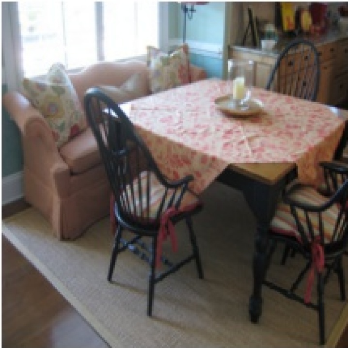
(a) Input

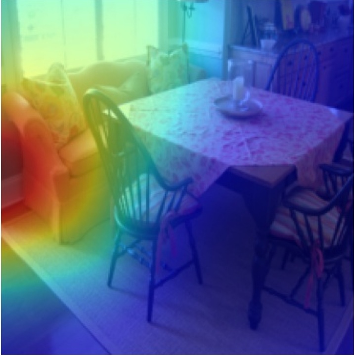
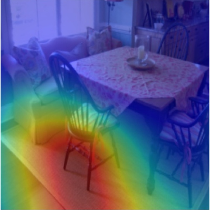
(b) BOREx

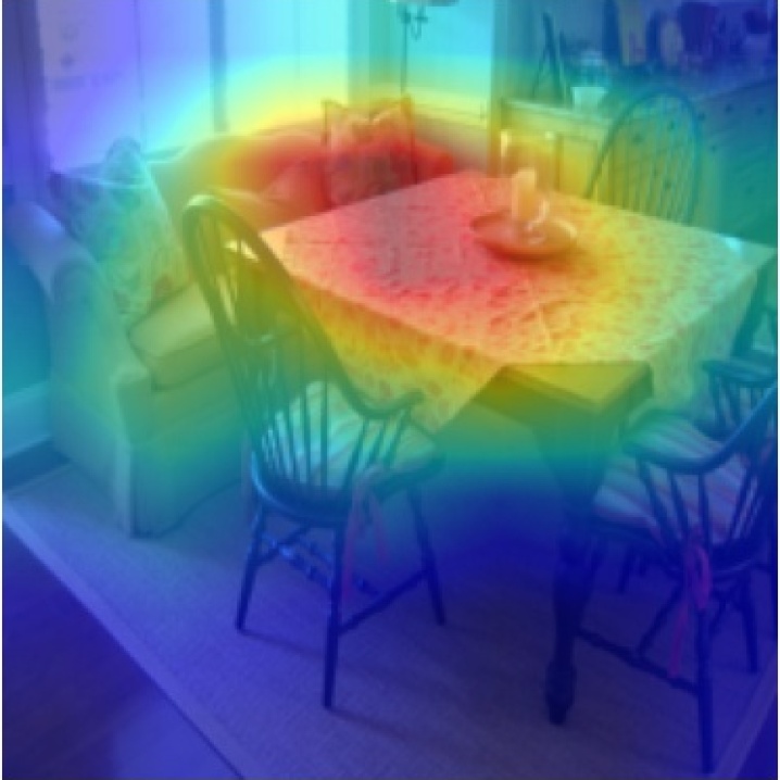
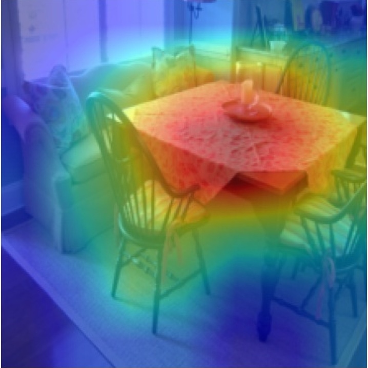
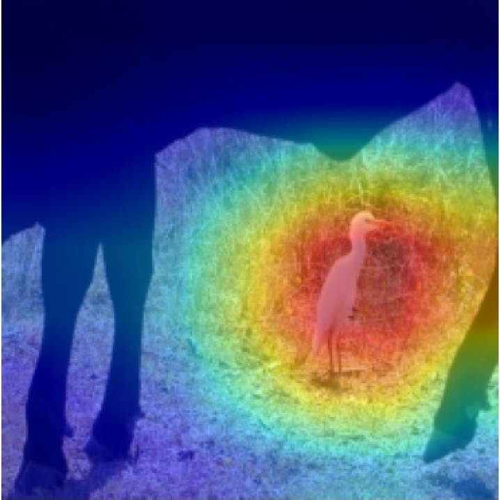
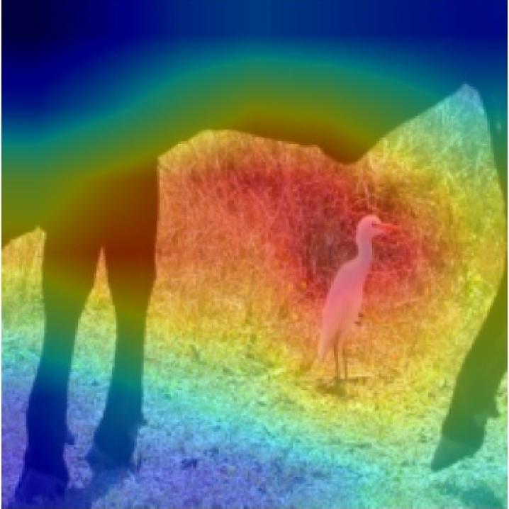
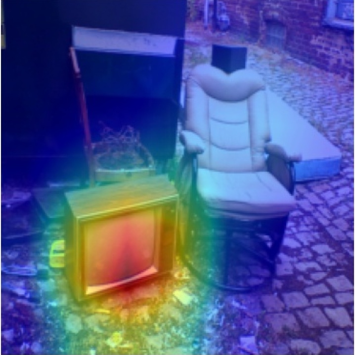
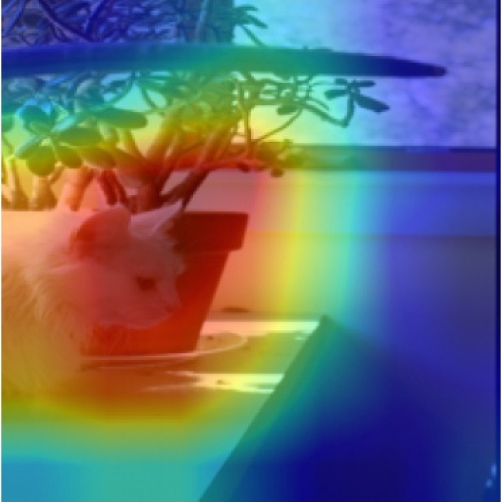
(c) Grad-CAM++

Figure 10: Examples of saliency maps in which BOREx outperforms GradCAM++. The labels used in each explanation are: “sofa”, “chair”, “bird”, “cow”, “chair”, “TV monitor”, and “potted plant”, from the first row.

Although the statistical tests in Section 4do not conclude the effectiveness of BOREx measured in the insertion and the F-measure metrics to refine the saliency map produced by Grad-CAM++, there are some instances that indeed benefit from BOREx. Figure 10 presents several examples of the saliency maps in which BOREx outperforms Grad-CAM++.

Interestingly, if we let BOREx and Grad-CAM++ produce saliency maps for the same image with different labels, the saliency maps produced by Grad-CAM++ are often less sensitive to the change in the label than BOREx. For example, the first (resp., the second) row in Figure 10 are the saliency maps produced by BOREx and Grad-CAM++ with label “sofa” (resp., “chair”). The saliency maps produced by BOREx correctly identify the region that is important for classifying the image to the given label; however, the saliency maps produced by Grad-CAM++ is less focused to the given label than BOREx.

Appendix 0.E Examples of saliency maps for video classifiers

(a) Input

(b) BOREx

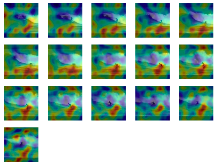
(c) RISE

(d) Grad-CAM++

Figure 11: Examples of saliency maps for video classifiers with label “surfing”.

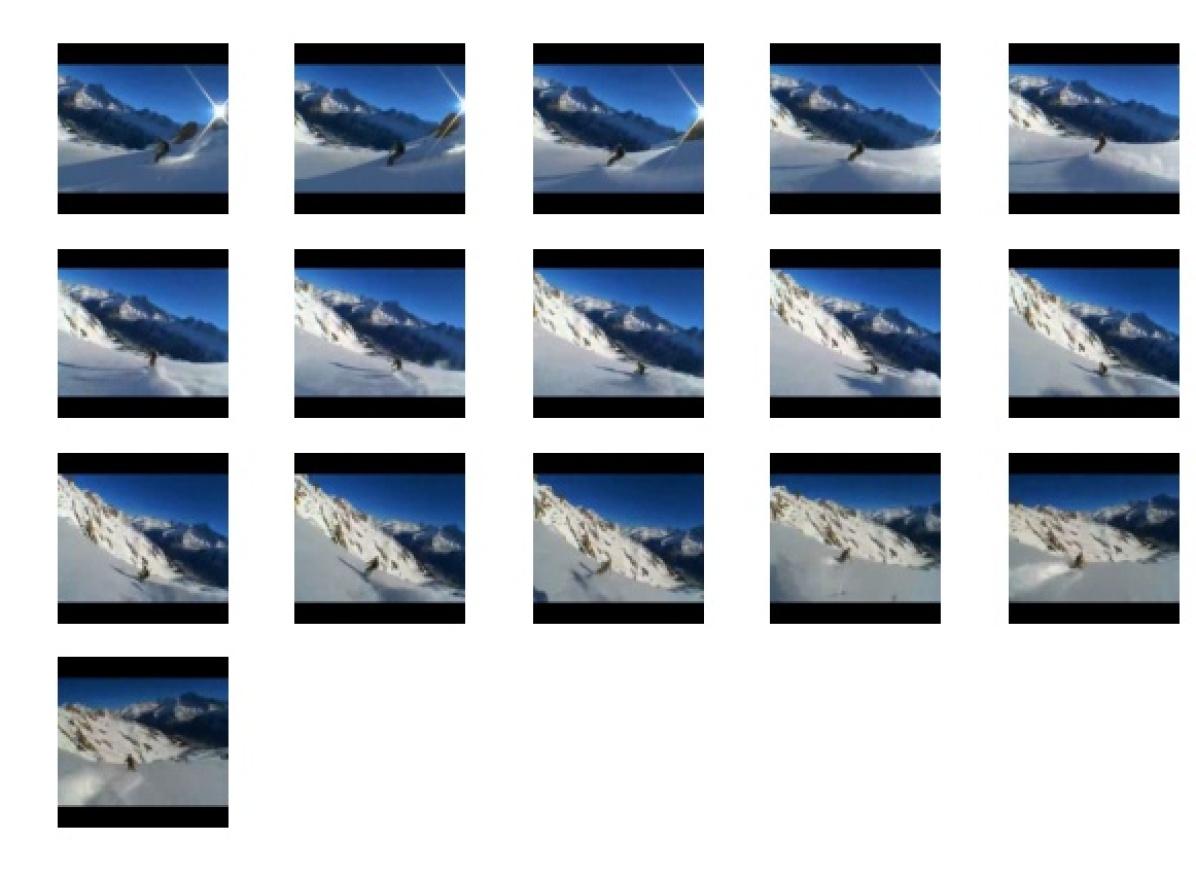
(a) Input

(b) BOREx

(c) RISE

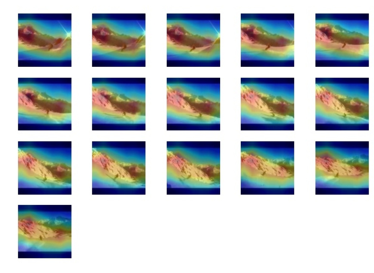
(d) Grad-CAM++

Figure 12: Examples of saliency maps for video classifiers with label “skiing”.

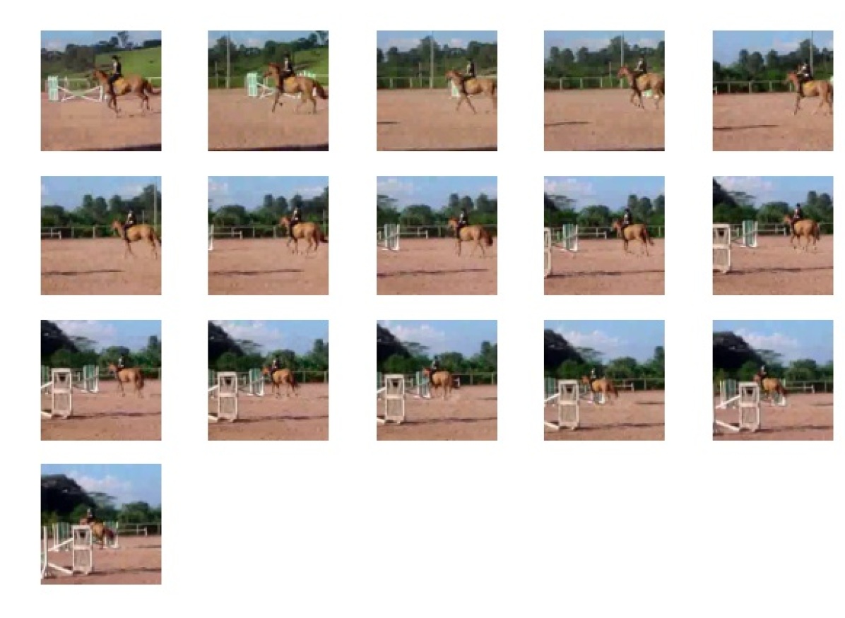
(a) Input

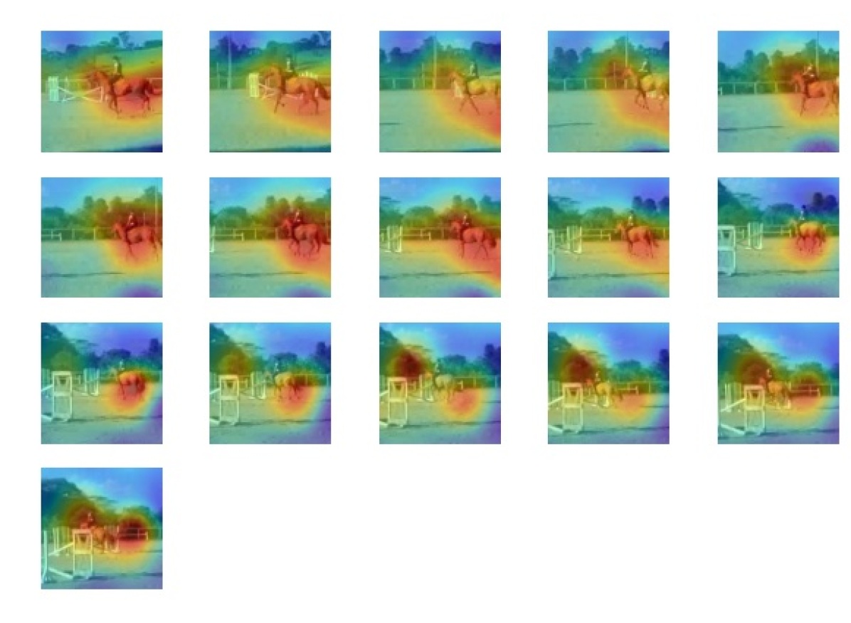
(b) BOREx

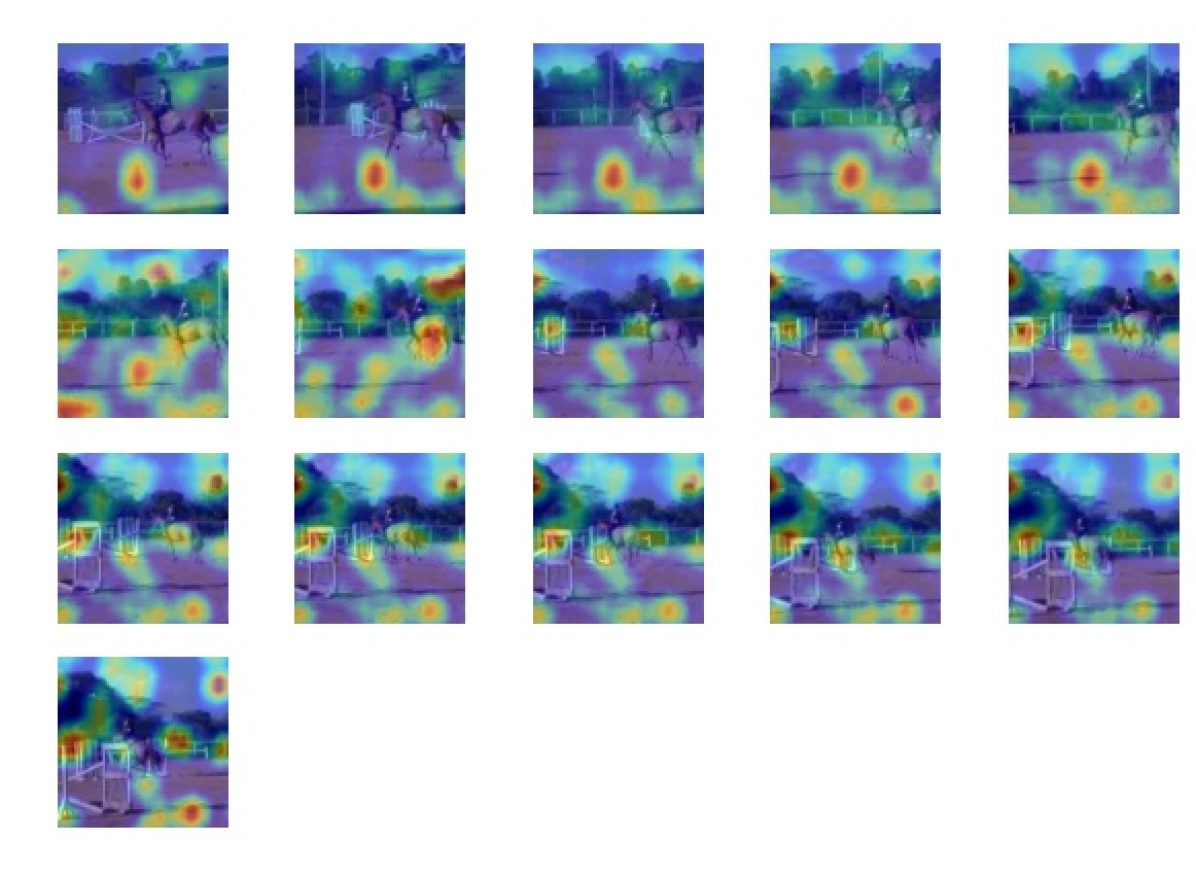
(c) RISE

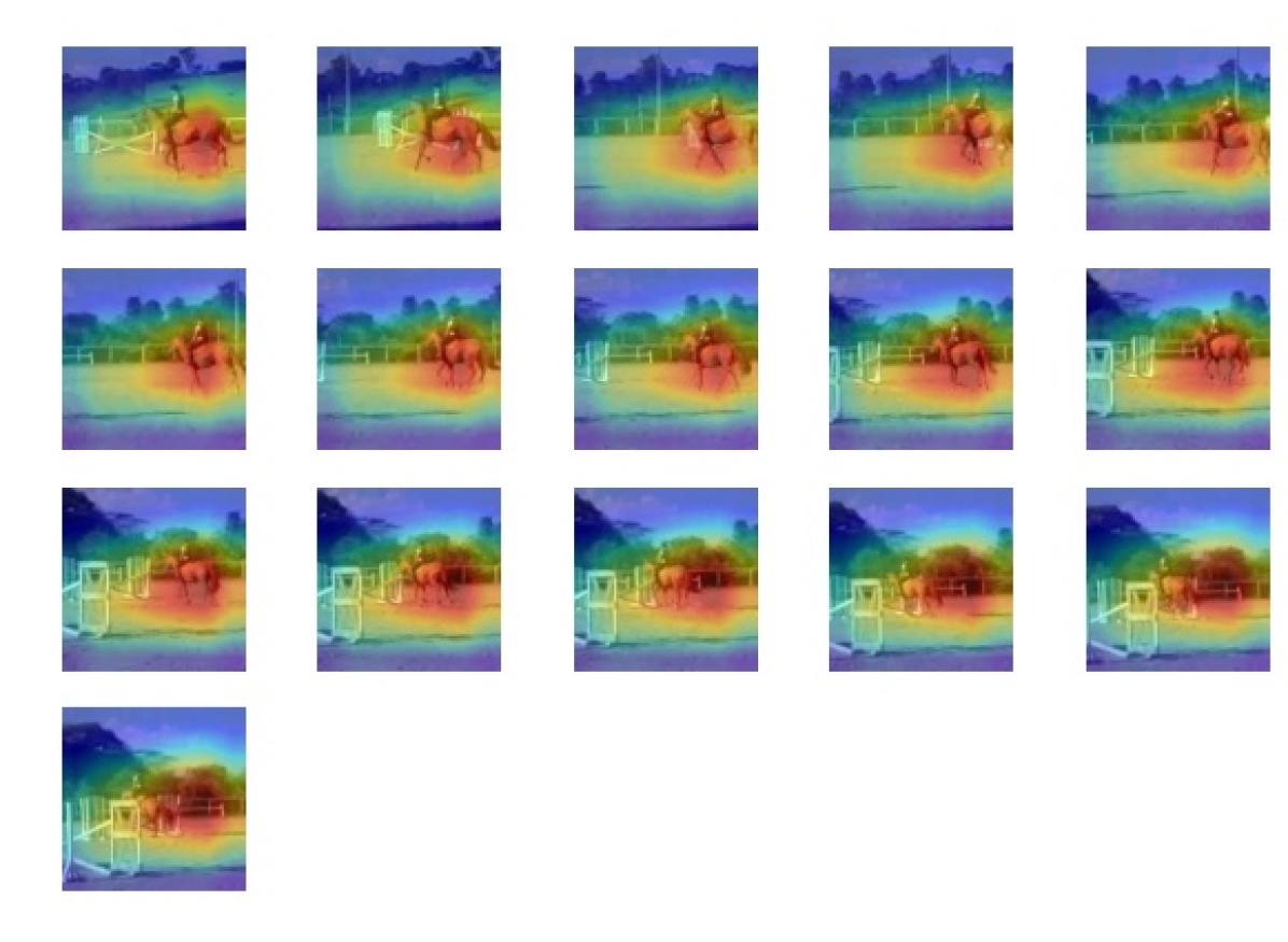
(d) Grad-CAM++

Figure 13: Examples of saliency maps for video classifiers with label “horseriding”.

Figures 11–13 present examples of saliency maps for a video classifier produced by BOREx and a naive extension of RISE. Compared with the saliency maps produced by RISE, the saliency maps generated by BOREx better localize the important parts. It is also observed that the salinecy maps produced by BOREx are comparable to those produced by Grad-CAM++ in spite of the black-box nature of BOREx. In Figure 12, we can observe that BOREx follows the skier better than Grad-CAM++.

References

- [1] Adebayo, J., Gilmer, J., Muelly, M., Goodfellow, I.J., Hardt, M., Kim, B.: Sanity checks for saliency maps. In: Advances in Neural Information Processing Systems 31: Annual Conference on Neural Information Processing Systems 2018, NeurIPS 2018, December 3-8, 2018, Montréal, Canada. pp. 9525–9536 (2018), https://proceedings.neurips.cc/paper/2018/hash/294a8ed24b1ad22ec2e7efea049b8737-Abstract.html
- [2] Bargal, S.A., Zunino, A., Kim, D., Zhang, J., Murino, V., Sclaroff, S.: Excitation backprop for RNNs. In: 2018 IEEE Conference on Computer Vision and Pattern Recognition, CVPR 2018, Salt Lake City, UT, USA, June 18-22, 2018. pp. 1440–1449 (2018). https://doi.org/10.1109/CVPR.2018.00156, http://openaccess.thecvf.com/content_cvpr_2018/html/Bargal_Excitation_Backprop_for_CVPR_2018_paper.html
- [3] Brunke, L., Agrawal, P., George, N.: Evaluating input perturbation methods for interpreting CNNs and saliency map comparison. In: Bartoli, A., Fusiello, A. (eds.) Computer Vision - ECCV 2020 Workshops - Glasgow, UK, August 23-28, 2020, Proceedings, Part I. Lecture Notes in Computer Science, vol. 12535, pp. 120–134. Springer (2020). https://doi.org/10.1007/978-3-030-66415-2_8, https://doi.org/10.1007/978-3-030-66415-2_8
- [4] Carreira, J., Zisserman, A.: Quo vadis, action recognition? A new model and the kinetics dataset. In: 2017 IEEE Conference on Computer Vision and Pattern Recognition, CVPR 2017, Honolulu, HI, USA, July 21-26, 2017. pp. 4724–4733 (2017). https://doi.org/10.1109/CVPR.2017.502, https://doi.org/10.1109/CVPR.2017.502
- [5] Chattopadhyay, A., Sarkar, A., Howlader, P., Balasubramanian, V.N.: Grad-CAM++: Generalized gradient-based visual explanations for deep convolutional networks. In: 2018 IEEE Winter Conference on Applications of Computer Vision, WACV 2018, Lake Tahoe, NV, USA, March 12-15, 2018. pp. 839–847. IEEE Computer Society (2018). https://doi.org/10.1109/WACV.2018.00097, https://doi.org/10.1109/WACV.2018.00097
- [6] Deng, J., Dong, W., Socher, R., Li, L., Li, K., Fei-Fei, L.: ImageNet: A large-scale hierarchical image database. In: 2009 IEEE Computer Society Conference on Computer Vision and Pattern Recognition (CVPR 2009), 20-25 June 2009, Miami, Florida, USA. pp. 248–255 (2009). https://doi.org/10.1109/CVPR.2009.5206848, https://doi.org/10.1109/CVPR.2009.5206848
- [7] Dombrowski, A., Alber, M., Anders, C.J., Ackermann, M., Müller, K., Kessel, P.: Explanations can be manipulated and geometry is to blame. In: Advances in Neural Information Processing Systems 32: Annual Conference on Neural Information Processing Systems 2019, NeurIPS 2019, December 8-14, 2019, Vancouver, BC, Canada. pp. 13567–13578 (2019), https://proceedings.neurips.cc/paper/2019/hash/bb836c01cdc9120a9c984c525e4b1a4a-Abstract.html
- [8] Everingham, M., Van Gool, L., Williams, C.K.I., Winn, J., Zisserman, A.: The pascal visual object classes (VOC) challenge. International Journal of Computer Vision 88(2), 303–338 (Jun 2010)
- [9] Ghorbani, A., Abid, A., Zou, J.Y.: Interpretation of neural networks is fragile. In: The Thirty-Third AAAI Conference on Artificial Intelligence, AAAI 2019, The Thirty-First Innovative Applications of Artificial Intelligence Conference, IAAI 2019, The Ninth AAAI Symposium on Educational Advances in Artificial Intelligence, EAAI 2019, Honolulu, Hawaii, USA, January 27 - February 1, 2019. pp. 3681–3688. AAAI Press (2019). https://doi.org/10.1609/aaai.v33i01.33013681, https://doi.org/10.1609/aaai.v33i01.33013681
- [10] Hatakeyama, Y., Sakuma, H., Konishi, Y., Suenaga, K.: Visualizing color-wise saliency of black-box image classification models. In: Ishikawa, H., Liu, C., Pajdla, T., Shi, J. (eds.) Computer Vision - ACCV 2020 - 15th Asian Conference on Computer Vision, Kyoto, Japan, November 30 - December 4, 2020, Revised Selected Papers, Part III. Lecture Notes in Computer Science, vol. 12624, pp. 189–205. Springer (2020). https://doi.org/10.1007/978-3-030-69535-4_12, https://doi.org/10.1007/978-3-030-69535-4_12
- [11] He, K., Zhang, X., Ren, S., Sun, J.: Deep residual learning for image recognition. In: 2016 IEEE Conference on Computer Vision and Pattern Recognition, CVPR 2016, Las Vegas, NV, USA, June 27-30, 2016. pp. 770–778 (2016). https://doi.org/10.1109/CVPR.2016.90, https://doi.org/10.1109/CVPR.2016.90
- [12] Heo, J., Joo, S., Moon, T.: Fooling neural network interpretations via adversarial model manipulation. In: Advances in Neural Information Processing Systems 32: Annual Conference on Neural Information Processing Systems 2019, NeurIPS 2019, December 8-14, 2019, Vancouver, BC, Canada. pp. 2921–2932 (2019), https://proceedings.neurips.cc/paper/2019/hash/7fea637fd6d02b8f0adf6f7dc36aed93-Abstract.html
- [13] Kay, W., Carreira, J., Simonyan, K., Zhang, B., Hillier, C., Vijayanarasimhan, S., Viola, F., Green, T., Back, T., Natsev, P., Suleyman, M., Zisserman, A.: The kinetics human action video dataset. CoRR abs/1705.06950 (2017), http://arxiv.org/abs/1705.06950
- [14] Li, Z., Wang, W., Li, Z., Huang, Y., Sato, Y.: Towards visually explaining video understanding networks with perturbation. In: Proc. of WACV 2021. pp. 1119–1128. IEEE (2021). https://doi.org/10.1109/WACV48630.2021.00116, https://doi.org/10.1109/WACV48630.2021.00116
- [15] Lundberg, S.M., Lee, S.: A unified approach to interpreting model predictions. In: Advances in Neural Information Processing Systems 30: Annual Conference on Neural Information Processing Systems 2017, December 4-9, 2017, Long Beach, CA, USA. pp. 4765–4774 (2017), https://proceedings.neurips.cc/paper/2017/hash/8a20a8621978632d76c43dfd28b67767-Abstract.html
- [16] Mokuwe, M., Burke, M., Bosman, A.S.: Black-box saliency map generation using bayesian optimisation. In: 2020 International Joint Conference on Neural Networks, IJCNN 2020, Glasgow, United Kingdom, July 19-24, 2020. pp. 1–8. IEEE (2020). https://doi.org/10.1109/IJCNN48605.2020.9207343, https://doi.org/10.1109/IJCNN48605.2020.9207343
- [17] Petsiuk, V., Das, A., Saenko, K.: RISE: Randomized input sampling for explanation of black-box models. In: British Machine Vision Conference 2018, BMVC 2018, Newcastle, UK, September 3-6, 2018. p. 151. BMVA Press (2018), http://bmvc2018.org/contents/papers/1064.pdf
- [18] Price, W., Damen, D.: Play fair: Frame attributions in video models. In: Ishikawa, H., Liu, C., Pajdla, T., Shi, J. (eds.) Computer Vision - ACCV 2020 - 15th Asian Conference on Computer Vision, Kyoto, Japan, November 30 - December 4, 2020, Revised Selected Papers, Part V. Lecture Notes in Computer Science, vol. 12626, pp. 480–497. Springer (2020). https://doi.org/10.1007/978-3-030-69541-5_29, https://doi.org/10.1007/978-3-030-69541-5_29
- [19] Rasmussen, C.E., Williams, C.K.I.: Gaussian Process for Machine Learning. The MIT Press (2006)
- [20] Ribeiro, M.T., Singh, S., Guestrin, C.: ”Why should I trust you?”: Explaining the predictions of any classifier. In: Proceedings of the 22nd ACM SIGKDD International Conference on Knowledge Discovery and Data Mining, San Francisco, CA, USA, August 13-17, 2016. pp. 1135–1144 (2016). https://doi.org/10.1145/2939672.2939778, https://doi.org/10.1145/2939672.2939778
- [21] Selvaraju, R.R., Cogswell, M., Das, A., Vedantam, R., Parikh, D., Batra, D.: Grad-CAM: Visual explanations from deep networks via gradient-based localization. Int. J. Comput. Vis. 128(2), 336–359 (2020). https://doi.org/10.1007/s11263-019-01228-7, https://doi.org/10.1007/s11263-019-01228-7
- [22] Shi, X., Khademi, S., Li, Y., van Gemert, J.: Zoom-CAM: Generating fine-grained pixel annotations from image labels. In: 25th International Conference on Pattern Recognition, ICPR 2020, Virtual Event / Milan, Italy, January 10-15, 2021. pp. 10289–10296 (2020). https://doi.org/10.1109/ICPR48806.2021.9412980, https://doi.org/10.1109/ICPR48806.2021.9412980
- [23] Stergiou, A., Kapidis, G., Kalliatakis, G., Chrysoulas, C., Veltkamp, R.C., Poppe, R.: Saliency tubes: Visual explanations for spatio-temporal convolutions. In: 2019 IEEE International Conference on Image Processing, ICIP 2019, Taipei, Taiwan, September 22-25, 2019. pp. 1830–1834 (2019). https://doi.org/10.1109/ICIP.2019.8803153, https://doi.org/10.1109/ICIP.2019.8803153
- [24] Subramanya, A., Pillai, V., Pirsiavash, H.: Fooling network interpretation in image classification. In: 2019 IEEE/CVF International Conference on Computer Vision, ICCV 2019, Seoul, Korea (South), October 27 - November 2, 2019. pp. 2020–2029 (2019). https://doi.org/10.1109/ICCV.2019.00211, https://doi.org/10.1109/ICCV.2019.00211
- [25] Tomsett, R., Harborne, D., Chakraborty, S., Gurram, P., Preece, A.D.: Sanity checks for saliency metrics. In: The Thirty-Fourth AAAI Conference on Artificial Intelligence, AAAI 2020, The Thirty-Second Innovative Applications of Artificial Intelligence Conference, IAAI 2020, The Tenth AAAI Symposium on Educational Advances in Artificial Intelligence, EAAI 2020, New York, NY, USA, February 7-12, 2020. pp. 6021–6029. AAAI Press (2020), https://aaai.org/ojs/index.php/AAAI/article/view/6064
- [26] Woolson, R.F.: Wilcoxon signed-rank test. Wiley encyclopedia of clinical trials pp. 1–3 (2007)
- [27] Zhang, J., Bargal, S.A., Lin, Z., Brandt, J., Shen, X., Sclaroff, S.: Top-down neural attention by excitation backprop. Int. J. Comput. Vis. 126(10), 1084–1102 (2018). https://doi.org/10.1007/s11263-017-1059-x, https://doi.org/10.1007/s11263-017-1059-x
- [28] Zhou, B., Khosla, A., Lapedriza, À., Oliva, A., Torralba, A.: Learning deep features for discriminative localization. In: 2016 IEEE Conference on Computer Vision and Pattern Recognition, CVPR 2016, Las Vegas, NV, USA, June 27-30, 2016. pp. 2921–2929 (2016). https://doi.org/10.1109/CVPR.2016.319, https://doi.org/10.1109/CVPR.2016.319