Empirical Macroeconomics and DSGE Modeling in Statistical Perspective

Abstract

Dynamic stochastic general equilibrium (DSGE) models have been an ubiquitous, and controversial, part of macroeconomics for decades. In this paper, we approach DSGEs purely as statstical models. We do this by applying two common model validation checks to the canonical Smets and Wouters (2007) DSGE: (1) we simulate the model and see how well it can be estimated from its own simulation output, and (2) we see how well it can seem to fit nonsense data. We find that (1) even with centuries’ worth of data, the model remains poorly estimated, and (2) when we swap series at random, so that (e.g.) what the model gets as the inflation rate is really hours worked, what it gets as hours worked is really investment, etc., the fit is often only slightly impaired, and in a large percentage of cases actually improves (even out of sample). Taken together, these findings cast serious doubt on the meaningfulness of parameter estimates for this DSGE, and on whether this specification represents anything structural about the economy. Constructively, our approaches can be used for model validation by anyone working with macroeconomic time series.

Keywords: general equilibrium; model validation; time series; forecasting;

1 Introduction

Since the 1980s, academic macroeconomics has been dominated by dynamic stochastic general equilibrium (DSGE) models, and economists have devoted a much attention to their specification, elaboration, mathematical manipulation, estimation, and theoretical refinement. This rise to prominence has been opposed, and there have always been critics of the whole approach on theoretical grounds, charging that, in one way or another, DSGE models are (or embody, or presume) bad economic theories. Instead of questioning whether DSGEs are good economics, we look at whether they are good models, i.e., whether they meet common, intuitive standards of statistical modeling.

In this paper, we are not primarily concerned with whether DSGE models can predict macroeconomic variables outside of the time period used to estimate their parameters. Out-of-sample forecasting is a quite elementary test of any statistical model’s actual fit to the data (Hastie et al., 2009), and this has been appreciated for a very long time (Stone, 1974; Geisser, 1975; Geisser and Eddy, 1979). Moreover, it’s well-established that DSGEs are bad at it (Edge and Gurkaynak, 2010), and even vector autoregressions do much better. We thus take it for granted that DSGEs are currently no good for prediction, and ask whether they will ever be capable of accurate forecasts. By the simple, standard device of simulating a DSGE and then fitting the same model to the simulation output, we show (sec. 3 below) that even when correctly specified in their entirety and provided with centuries of simulated data, these models remain incapable of forecasting. Worse, their parameters remain very badly estimated. To reliably estimate models of such coelenterate flexibility would require thousands of years (at least) of data from a stationary economy.

We are aware that many economists downplay using DSGEs for prediction on the grounds that the models are instead supposed to inform us about the structure of the economy and about the consequences of prospective policy interventions. Even if this is true, however, one would need some reason to think that this DSGE, rather than another, was getting things right. While we agree that models which are capable of accurate statistical prediction may be horrible at causal, counter-factual prediction, it has long been understood that the reverse is not true (Spirtes et al., 1993; Pearl, 2000), and this is now literally a textbook point in causal inference (Morgan and Winship, 2015). A model which gets the causal structure right, and can make accurate counter-factual predictions, should a fortiori be capable of accurate statistical prediction as well. Hence economists’ confidence in their favorite DSGEs suitability for policy evaluation cannot be rooted in their statistical predictive ability, since the later does not exist.

We also undermine the notion that DSGE specifications capture the structure of the economy by the simple expedient of swapping the different time series on which they are fit — giving the model as “investment” the series that is really “hours worked”, and so forth (sec. 4 below). Not only does such series swapping do little to degrade the DSGE’s performance, in sample or out of sample, in a large fraction of permutations it actually enhances predictability. It is, of course, open to an economist to maintain their belief in a favorite DSGE’s capturing the structure of the macroeconomy even if it cannot predict, and cannot tell the difference between the real data and one with all the series swapped, but such faith truly is maintained on the evidence of things not seen.

The principles to which we appeal — using simulation to assess estimation methods; using randomization to gauge how well a model can appear to fit nonsense data — are not recondite points of mathematical theory, and involve no controversial questions in the foundations of statistics. Rather, they are readily explained notions, accepted on pretty much all sides within modern statistics, whose force is easily grasped once they are presented. We return to their implications for macroeconomic modeling in the conclusion.

1.1 Brief Remarks on the Literature

There is a familiar story to the rise of DSGEs from the 1970s to the 1990s, which roots them in, on the one hand, the desire to give “microfoundations” to macroeconomic models, and, on the other hand, the Lucas (1976) critique of “old Keynesian” models, and the latter’s apparent empirical failure in the 1970s. The breakthrough paper, on this account, was the “real business cycle” model of Kydland and Prescott (1982). Versions of this story are familiar from textbooks (e.g., DeJong and Dave 2011), and it’s not our place here to dispute it. It is undeniably true that, following Kydland and Prescott (1982), macroeconomists rapidly cultivated many breeds of DSGE model, embodying a range of substantive economic assumptions, but also conserving certain crucial features that define the lineage, such as the use of representative agents (often just one representative agent) in equilibrium. The motivation was also conserved: DSGEs (it is held) clearly separate enduring, “structural” aspects of the economy, ultimately relating to tastes, technologies and institutions, from policy and from fluctuations. The structural, tastes-and-technologies aspects are held to be invariant, at least to policy and at least over the relevant time scales. Embedding these into a dynamic equilibrium model is supposed to get around the Lucas critique, by ensuring that even if the predictions of the model are known and are used as the basis of policy, the model will remain valid, because it describes an equilibrium over time.

The model we focus on, that of Smets and Wouters (2007), hereafter denoted SW, while now some years old, is still widely regarded as an acceptable baseline model. A great deal of macroeconomic theorizing thus consists of taking this model, or other very similar ones, and elaborating on them by adding new frictions or shocks. These additions are generally intended to accommodate observed phenomena, to incorporate conjectured mechanisms, or both. It is not our purpose here to comment on specific descendants of the SW or other baseline DSGE models. We merely note that the strategy of responding to issues or defects with the model by always making it more complex (more frictions, more shocks, etc.) is at least questionable from a statistical perspective.

As we wrote in the introduction, our objective here is not to add to the literature for or against DSGE models from the viewpoint of economic theory. It is not even pertinent to survey that voluminous, often acrimonious, literature. We take no sides, here, on whether agents in macroeconomic models should be assumed to have rational (rather than adaptive) expectations, should have perfect (rather than bounded) rationality, should (or should not) obey the Euler equations, etc. We do not even take a side on whether aggregating large numbers of heterogeneous economic actors into a few representative agents is in fact “microfounded”. Those who are a priori inclined to dismiss DSGEs as inappropriate models will, we suspect, find our results on their statistical difficulties congenial. But no result we are aware of implies that theoretically sound economic models must also have good statistical properties. Moreover, for all we know at this stage, all the proposed alternatives to DSGEs also suffer from the same statistical flaws! (We invite their partisans, or perhaps their enemies, to check.)

Turning to the literature on statistical properties of DSGEs, this has mostly focused on issues of estimation and testing; we cite specific works below as needed. A smaller body of work has examined out-of-sample forecasting ability of DSGEs, notably Edge and Gurkaynak (2010) (see also references therein). That paper found that these model predicted poorly, but ingeniously attributed this to the close control exercises by central bankers and other policy-makers. (Other explanations suggest themselves.) Another tangentially-relevant body of work has examined identification issues in DSGEs. The most important paper here is probably still Komunjer and Ng (2011), which gave fairly practical algebraic conditions for checking the identifiability of DSGEs. (This built off earlier work by Iskrev 2010 among others.) Identification means that all model parameters can (in principle) be estimated in the limit; estimates using the available, non-asymptotic amount of data might be unacceptably imprecise, and might converge unacceptably slowly. We are unaware of any previous work which has addressed the practical estimability of DSGEs by the means used here, or anything like it. We are also unaware of any previous work which probes whether DSGEs are actually capturing the structure of the macroeconomy by anything like the expedient of series swapping.

2 Specification and Baseline Estimation of the DSGE

In this section, we review how DSGE models work, the specification of the Smets and Wouters (2007) DSGE that serves as our test case, and some of the issues that arise in estimating the parameters of this model.

2.1 Solving DSGEs

A DSGE model is the solution to a constrained stochastic inter-temporal optimization problem

$$z_{t}^{*} =\operatorname*{argmax}\sum_{t=0}^{\infty}\mathbb{E}g(z_{t}) z_{t} =h(z_{t-1}),$$ s.t. (1)

for some nonlinear functions $g$ and $h$ parametrized by a $k$-dimensional vector of “deep” parameters $\theta$. The economic agents posited by the model are assumed to solve this problem (optimally) at each time $t$ conditional on all current and previously available information, and we observe part of the solution: that is the observable data are $x_{t}$ which is a subset of the indices of $z_{t}^{*}$.

To estimate a DSGE, the first step is to solve the optimization problem by deriving the first-order conditions for an optimum. The resulting nonlinear system can be written as

$$\Phi(z_{t},\ z_{t+1})=0,$$ (2)

for some $n$-dimensional function $\Phi$. Such systems can rarely be solved analytically for the optimal path; instead, the first-order conditions are used to express the model in terms of stationary variables, and the system is linearized around this steady-state (that is, let $z$ be the vector satisfying $z=z_{t}=z_{t-1}$). Upon writing $z_{t}=z^{*}_{t}-z$, the (linearized) DSGE can be written as

$$\Gamma_{0}z_{t}=\Gamma_{1}z_{t-1}+A+B\epsilon_{t}+C\eta_{t}$$ (3)

in the notation of Sims (2002). Here $\epsilon_{t}$ are exogenous, possibly serially correlated, random disturbances and $\eta_{t}=z_{t}-\mathbb{E}_{t}z_{t+1}$ are expectational errors determined as part of the model solution. The matrices $\Gamma_{0}$, $\Gamma_{1}$, $A$, $B$, and $C$ are functions of $\theta$.

There are a number of ways to estimate $\theta$ using data; a complete treatment is beyond our scope here, but see DeJong and Dave (2011) for details. We will focus on likelihood-based approaches, and so we must solve the model in equation (3). There are many approaches to solving linear rational expectations models (e.g. Blanchard and Kahn, 1980; Klein, 2000), but we will use that in Sims (2002) due to its ubiquity. This method essentially uses a QZ factorization to remove $\Gamma_{0}$ from the left side of the equation while correctly handling explosive components of the model (merely multiplying through by the generalized inverse of $\Gamma_{0}$, $\Gamma_{0}^{\dagger}$, can lead to portions of the product $\Gamma_{0}^{\dagger}\Gamma_{1}$ implying nonstationarity). Following this procedure, we retrieve a system of the form

$$z_{t}=d+Tz_{t-1}+H\varsigma_{t}$$ (4)

as long as there is a unique mapping from equation (3) (there may be multiple solutions or none depending on $\theta$). Since some of the $z_{t}$ are unobserved, we augment the transition equation in (4) with an observation equation

$$x_{t}=Zz_{t},$$ (5)

where the matrix $Z$ subselects the appropriate elements of $z_{t}$. Collecting equations (4) and (5) gives the form of a linear state-space model. Assuming that the errors $\varsigma_{t}$ are serially independent multivariate Gaussian allows us to evaluate the likelihood of some parameter vector $\theta$ given observed data $x_{1},\ldots,x_{T}$. Evaluating the likelihood can be done using the Kalman filter (Kalman, 1960) which is readily available in most software packages. The procedure outlined above is summarized in Algorithm 1.

1:Write down DSGE as a constrained optimization problem.

2:Determine the first order conditions for an optima.

3:Determine steady state path of observables.

4:Linearize the DSGE around the steady-state yielding a general form for (3).

5:procedure Estimate the model($\theta$)

6:     Fix a plausible parameter vector $\theta$.

7:     For this $\theta$, cast (3) into state-space form using the method of Sims (2002).

8:     Using equations (4) and (5), evaluate the likelihood of $\theta$ using the Kalman filter.

9:     Maximize the likelihood or explore the posterior, repeating as needed at new values of $\theta$.

10:end procedure

Algorithm 1 Pseudoalgorithm for estimating linear rational expectations models

2.2 Estimating the Smets and Wouters (2007) model

In this section, we provide a description of the procedure we use for estimating the Smets and Wouters (2007) model. The model is now standard in the macroeconomic forecasting literature, and, though code is readily available (for example in Dynare or Matlab), our version is implemented fully in R. A complete description of the economic implications of the model and its log-linearized form can be found in Smets and Wouters (2007) as well as Iskrev (2010) and other sources.

For this model, we use seven observable data series: output growth, consumption growth, investment growth, real wage growth, inflation, hours worked, and the nominal interest rate, which we collect into the vector $x_{t}$

$$x_{t}=\begin{bmatrix}y_{t}-y_{t-1}&c_{t}-c_{t-1}&i_{t}-i_{t-1}&w_{t}-w_{t-1}&\pi_{t}&l_{t}&r_{t}\end{bmatrix}^{\top}.$$ (6)

We describe the specific data and preprocessing routines in Appendix A, but we note that all the data are publicly available from the Federal Reserve Economic Database (FRED). We use data from the first quarter of 1956 until the fourth quarter of 2018. Following preprocessing, we are left with 251 available time points.

The model has 52 “deep” parameters as well as 7 parameters representing the standard deviations of the stochastic shocks. Of these 59 total parameters, we estimate 36: 18 are derived from steady-state values as functions of other parameters and 5 are fixed a priori (as in Smets and Wouters 2007). The prior distributions for the 36 estimated parameters are given in Table 1. To estimate the model we minimize the negative log likelihood, penalized by the prior. This is the same as finding the maximum a posteriori estimate in a Bayesian setting. Because the likelihood is ill-behaved, having many flat sections as well as local minima, we used R’s optimr package. We estimated the parameter using both the simulated annealing method, which stochastically explores the likelihood surface in a principled manner, and the conjugate gradient technique. Each procedure was started at 5 random initializations (drawn from the prior distribution) and run for 50,000 iterations (likelihood evaluations) for each starting point. We train the model using only the first 200 time points, saving the remainder to evaluate the model’s (pseudo-out-of-sample) predictive performance.

Table 1 presents the posterior mode based on our procedure. Note first that some of the parameter estimates are similar to those presented in Smets and Wouters (2007) (shown in the last column), while others differ dramatically. However, comparing the likelihood of of our estimated parameters to those in Smets and Wouters (2007), our fit is significantly better. For our dataset, the penalized negative log likelihood of the parameters is 1145 compared to 1232, an improvement of more than 7.1%. The result is similar for the unpenalized negative log likelihood. To check for robustness, we also ran the optimization procedure for 1 million parameter draws and the likelihood only decreased by about 1%. We are therefore confident that we have a parameter combination which nearly achieves the global optimum.

Table 1: Prior distributions, posterior modes, and posterior mode as estimated by Smets and Wouters (2007) for the 36 estimated parameters. All values are rounded to two decimal places.

	prior distribution	prior mean	prior stdev	lower bound	upper bound	posterior mode	SW posterior mode
$\sigma_{a}$	igamma	0.10	2.00	0.01	3.00	0.44	0.45
$\sigma_{b}$	igamma	0.10	2.00	0.03	5.00	0.30	0.24
$\sigma_{g}$	igamma	0.10	2.00	0.01	3.00	0.57	0.52
$\sigma_{I}$	igamma	0.10	2.00	0.01	3.00	0.48	0.45
$\sigma_{r}$	igamma	0.10	2.00	0.01	3.00	0.22	0.24
$\sigma_{p}$	igamma	0.10	2.00	0.01	3.00	0.15	0.14
$\sigma_{w}$	igamma	0.10	2.00	0.01	3.00	0.27	0.24
$\rho_{a}$	beta	0.50	0.20	0.01	1.00	0.97	0.95
$\rho_{b}$	beta	0.50	0.20	0.01	1.00	0.14	0.18
$\rho_{g}$	beta	0.50	0.20	0.01	1.00	0.95	0.97
$\rho_{I}$	beta	0.50	0.20	0.01	1.00	0.66	0.71
$\rho_{r}$	beta	0.50	0.20	0.01	1.00	0.13	0.12
$\rho_{p}$	beta	0.50	0.20	0.01	1.00	0.99	0.90
$\rho_{w}$	beta	0.50	0.20	0.00	1.00	0.95	0.97
$\mu_{p}$	beta	0.50	0.20	0.01	1.00	0.88	0.74
$\mu_{w}$	beta	0.50	0.20	0.01	1.00	0.90	0.88
$\phi_{1}$	gaussian	4.00	1.50	2.00	15.00	5.73	5.48
$\sigma_{c}$	gaussian	1.50	0.38	0.25	3.00	1.55	1.39
$h$	beta	0.70	0.10	0.00	0.99	0.72	0.71
$\xi_{w}$	beta	0.50	0.10	0.30	0.95	0.78	0.73
$\sigma_{l}$	gaussian	2.00	0.75	0.25	10.00	2.01	1.92
$\xi_{p}$	beta	0.50	0.10	0.50	0.95	0.60	0.65
$\iota_{w}$	beta	0.50	0.15	0.01	0.99	0.34	0.59
$\iota_{p}$	beta	0.50	0.15	0.01	0.99	0.26	0.22
$\Psi$	beta	0.50	0.15	0.01	1.00	0.57	0.54
$\Phi$	gaussian	1.25	0.12	1.00	3.00	1.13	1.61
$r_{\pi}$	gaussian	1.50	0.25	1.00	3.00	2.06	2.03
$\rho$	beta	0.75	0.10	0.50	0.98	0.83	0.81
$r_{y}$	gaussian	0.12	0.05	0.00	0.50	0.10	0.08
$r_{\Delta y}$	gaussian	0.12	0.05	0.00	0.50	0.21	0.22
$\overline{\pi}$	gamma	0.62	0.10	0.10	2.00	0.63	0.81
$100(\beta^{-1}-1)$	gamma	0.25	0.10	0.01	2.00	0.13	0.16
$\overline{l}$	gaussian	0.00	2.00	-10.00	10.00	3.34	-0.10
$\overline{\gamma}$	gaussian	0.40	0.10	0.10	0.80	0.47	0.43
$\rho_{ga}$	gaussian	0.50	0.25	0.01	2.00	0.63	0.52
$\alpha$	gaussian	0.30	0.05	0.01	1.00	0.28	0.19

3 Simulate and estimate

A simple way to evaluate a stochastic model is to simulate a long time series from the model and see how well we can estimate the generating process given more and more data. In a sense, this is a minimal requirement for any model: does it produce consistent estimates of the true parameters? And furthermore, how much data will we need? Statistical theory for independent and identically distributed data says that maximum likelihood estimators for a fixed number of parameters are $n$-consistent in MSE. This is essentially as fast as we could hope. In this exercise, we abstract from the non-linear DSGE: supposing that the data were actually generated by the linearized DSGE represented by equations (4) and (5), can we recover the “deep” parameters which generated the data?

To answer this (relatively simple) question, we generate data using the parameters estimated above and presented in Table 1. To reduce dependence on initial conditions, we simulate 3100 data points and discard the first 1000. We then train the model using the first 100 data points (25 years worth of quarterly data), and try to predict the next 1000 to measure out-of-sample performance. We then increment forward 20 time-steps (5 years), train again and predict the next 1000 observations. We continue this process until we are using 1100 data points (275 years of data) to estimate the model. To average over simulation error, we repeat the entire exercise 100 times. For each estimation, we initialize the optimization procedure at the true parameter value and run it for 30000 iterations. This ensures that the true parameters are considered, maximizing the chance that the estimation will return the data generating values. Our goal here is to learn whether we could hope to learn the right parameters in 275 years’ time if the linearized DSGE is actually true, and furthermore, how well can we predict future economic movements under this idealized scenario.

All figures in this section show the mean in red along with 30%, 60%, 80%, and 90% confidence bands calculated from the replications.

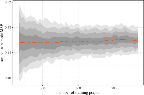
Figure 1: Training (in sample) error averaged across series as the number of training points increases. We would expect the variability to decline while the average remains constant. The mean is shown in red along with 30%, 60%, 80%, and 90% confidence bands calculated from the replications.

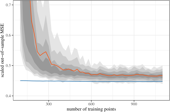
Figure 2: Out-of-sample error averaged across series as the number of training points increases. We would expect both the variability and the average to decline. The blue line is the test error for the true model.

Figure 1 shows the average training error (averaged across the 7 series). As we would expect, the variability declines as the size of the training set increases, though not the average. Figure 2 shows the average prediction error over the 7 series. It improves markedly as the training set increases to about 400 observations (=100 years) but then plateaus. This is troubling: as we get more and more data, we can not predict new data any better. This indicates one of three possibilities: (1) that with about 400 observations, we can estimate the parameters nearly perfectly, (2) that the model is poorly identified—some parameters will simply never be well estimated, but we can predict well anyway, or (3) the data are so highly correlated that the range of training observations we consider is far too small—we actually need millions of observations in order to see a meaningful decline in out-of-sample predictive performance. We can better determine which of these three is occurring by comparing with the predictive performance of the true parameters and examining the error in parameter estimates. The blue line in Figure 2 is the out-of-sample mean prediction error for the true parameters. The test error is not getting any closer to this ideal scenario, plateauing slightly above the baseline by about 400 training points. This seems to suggest that explanation (2) is accurate: even with more data, we will never be able to recover the true parameters, though we get some improvement in predictions relatively quickly.

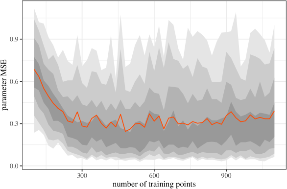
Figure 3: The parameter MSE shows similar behavior to the predictive MSE: steep initial decline toward an asymptote greater than that of the true model.

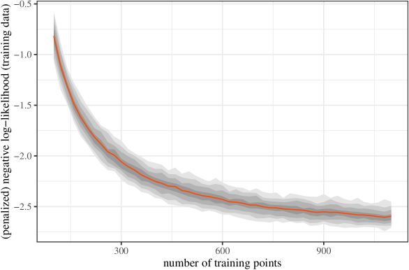
Figure 4: The negative log-likelihood (in-sample) per observation.

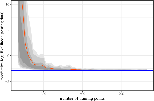
Figure 5: The negative predictive log-likelihood (out-of-sample) per observation.

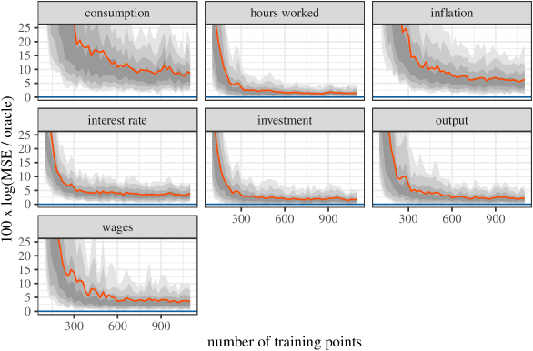
Figure 6: Mean-squared prediction error for each series.

Examining the parameter error serves to confirm this conjecture. Figure 3 shows the average squared error of the parameter estimates. Improvement in this metric also stagnates despite the growing training sets. Figure 4 and Figure 5 show the change in information per observation (in sample) and per prediction (out of sample). For maximum likelihood inference, we would expect both of these to decline as the amount of training data increases. These figures therefore confirm that the estimation procedure is responding to the increased sample size even though prediction and estimation errors both fail to improve meaningfully. Figure 6 shows the average prediction error for each series individually. From this decomposition, prediction of all time series improves, but only labor ever reaches the minimum (relative to the truth). The other series are all predicted poorly.

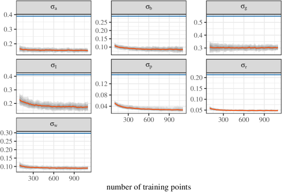
Figure 7: Estimates for the standard deviations of stochastic shocks.

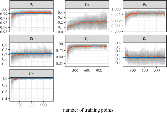
Figure 8: Estimates for the autocorrelation parameters in the shock processes.

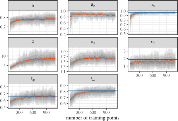
Figure 9: Estimates of ”deep” parameters

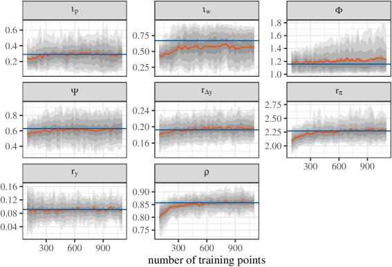
Figure 10: Estimates of ”deep” parameters

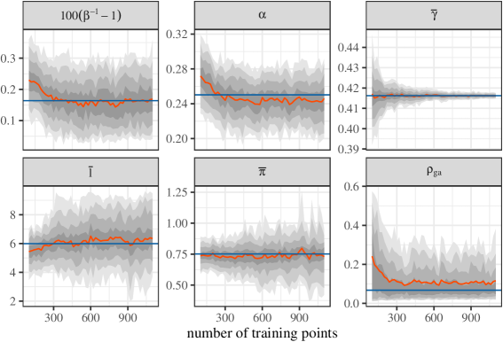
Figure 11: Estimates of ”deep” parameters

Figures 7–11 show the estimates of each parameter individually. The horizontal red lines indicate the truth. Here we can see that while many parameters are well-estimated with decreasing variability as the training sets grow, others converge to the wrong values, or fail to converge at all. This phenomenon holds especially for both of the parameters of the shock processes, but also for some of the economically-relevant “deep” parameters. For instance, $\sigma_{l}$, the elasticity of labor supply with respect to the real wage, is consistently underestimated by about -93%. The data provides essentially no information about $\iota_{w}$, which measures the dependence of real wages on lagged inflation. Other parameters which are poorly estimated include $\varphi$, the steady-state elasticity of the capital adjustment cost function. In all these cases, estimation is biased, so using the estimated values from the real data to draw conclusions about the real economy is unwise. It is possible that this bias is due to the linearization procedure, in which case, not only should linearized models be avoided for prediction, but also for drawing any economic inferences. Overall, most parameters are poorly identified as evidenced by their stable (rather than decreasing) variability with more data.

To examine case (3)—that the data is so correlated that even 250 years is too little to produce accurate estimates of the true parameters—we may ask how closely the information per observation displayed in Figure 4 approaches the theoretical asymptotic limit. For essentially any stationary ergodic stochastic process, the limit of the negative loglikelihood per observation as the number of observations approaches infinity exists and is unique (Gray, 2011). This limit is the entropy rate of the process. Mathematically, with probability 1,

$$\lim_{n\rightarrow\infty}-\frac{1}{n}\ell(X_{1:n};\theta_{0})=h(\theta_{0}),$$

where $h(\theta_{0})$ is the entropy rate. Furthermore, by the generalized asymptotic equipartition property (Algoet and Cover, 1988), one can show that for any other parameter vector $\theta\neq\theta_{0}$, with probability 1,

$$\lim_{n\rightarrow\infty}-\frac{1}{n}\ell(X_{1:n};\theta)=h(\theta_{0})+\mathrm{KL}(\theta_{0}\ ||\ \theta),$$

where the second term is the Kullback-Leibler divergence rate (Gray, 2011). Because $\mathrm{KL}(\theta_{0}\ ||\ \theta)\geq 0$, asymptotically, $h(\theta_{0})$ is a lower bound for the average negative loglikelihood of any parameter vector.

Because the data is generated from a linear Gaussian state space model, it is not hard to calculate that $h(\theta_{0})\approx 2.25$, significantly larger than any of the values in Figure 4. Somehow, the estimated parameters generally have lower negative loglikelihoods than the true parameter. The fact that the standard deviations of the shocks (Figure 7) are consistently underestimated suggests that, even over this period, the in-sample fit to the data gives an overly optimistic picture of the long run behavior: we have not allowed $n$ to get large enough. Figure 12 shows the negative loglikelihood per observation over a much longer horizon—up to 75,000 years of quarterly data. For thousands of years, the parameter vector estimated over the first 250 years is less than the theoretical lower bound, but eventually, it starts to curve upward. This suggests that, both explanations (2) and (3) are accurate: in order to estimate a DSGE accurately, we need massive amounts of data.

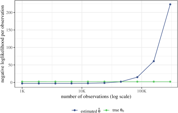
Figure 12: Comparing the in-sample negative loglikelihood per observation of a parameter estimated with 1000 observations relative to the true parameter. In the long-run, the entropy rate is a lower bound, but only after about 12,000 years of quarterly data.

4 Permuting the data

A second way to assess the predictive ability (and economic content) of the SW DSGE model is to perform a simple permutation test, permuting across the series rather than within them. That is, rather than giving the model data in the order it expects, we swap the data series with each other and see if the model predicts future data any better. We estimated the model on the properly ordered data (presented in the previous section) as well as all 5039 other permutations of the 7 data series. For each estimation, we used the same estimation procedure as before to minimize the (penalized) negative log likelihood. The model is trained using the first 200 time points and its predictive performance is tested on the remaining 51.

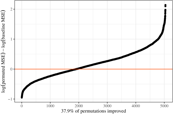
Figure 13: Average percentage improvement in out-of-sample forecast MSE. The horizontal red line represents baseline performance. Lower values are better.

The next few figures summarize the results. We report three criteria for measuring relative performance. The first is the percent improvement in (out-of-sample) mean-squared test error (MSE) calculated as the natural logarithm of the test error for a particular permutation divided by that of the baseline model and then averaged across all 7 series:

$$\mbox{Average Percent MSE Improvement (p)}=\frac{1}{7}\sum_{i=1}^{7}\log\left(\frac{\sum_{t=201}^{251}(\widehat{x}_{it}^{(p)}-x_{it})^{2}}{\sum_{t=201}^{251}(\widehat{x}_{it}^{b}-x_{it})^{2}}\right),$$ (7)

where a superscript $b$ represents the baseline model and $(p)$ the $p^{th}$ permutation. The result is shown in Figure 13. Figure 14 shows boxplots for the percentage improvement separately for each time series. The best model had an average percentage improvement of 95% relative to the baseline model. The vertical line at zero represents performance equivalent to baseline. About 38% of permutations had better predictive performance than the baseline model.

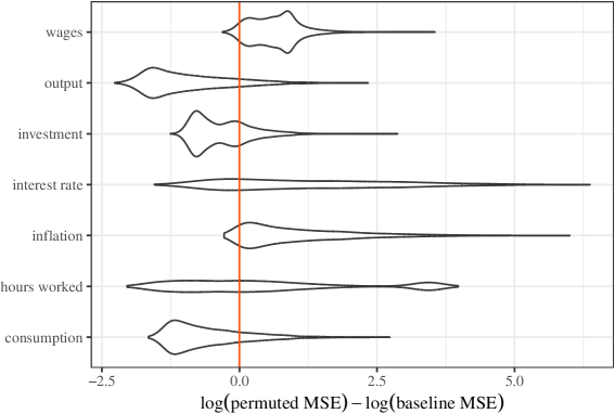
Figure 14: Percentage improvement in out-of-sample forecast MSE for each data series individually. The horizontal red line represents baseline performance. Values to the left are better.

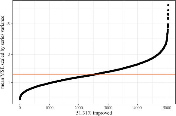
Figure 15: Average improvement in out-of-sample forecast MSE scaled by the variance of the data. The horizontal red line represents baseline performance.

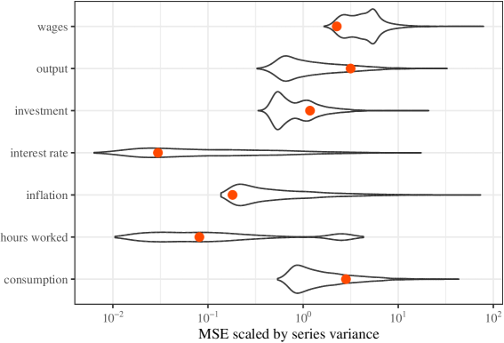
Figure 16: Improvement in out-of-sample forecast MSE scaled by the variance of the data for each data series individually. The red dots represents baseline performance.

The second measure of performance is simply the out-of-sample MSE scaled by the observed variance and then averaged across the 7 series:

$$\mbox{Average Scaled MSE (p)}=\frac{1}{7}\sum_{i=1}^{7}\frac{\sum_{t=201}^{251}(\widehat{x}_{it}^{(p)}-x_{it})^{2}}{\mbox{Var}(x_{i})}.$$ (8)

Figure 15 displays the average of this measure across all 251 series. Again, about 51% of permutations achieved better average scaled MSE than the baseline model. The best permutation achieved an average scaled MSE of 0.53 relative to 1.39 for the baseline model. Figure 16 shows boxplots for the scaled MSE separately for each series. Red dots indicate the performance of the baseline model.

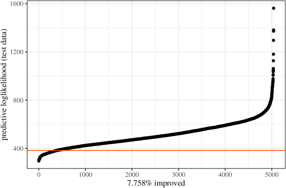
Figure 17: Negative log predictive likelihood for each model. The horizontal red line represents baseline performance. Note that this is an out-of-sample performance measure.

A total of 0 of permutations resulted in a lower negative penalized log likelihood. A Bayesian interpretation of these results would be that 0 of the permuted “models” are preferable to the true, unpermuted, economic model. It should be noted that this is an in-sample measure of performance and that the Bayesian interpretation is conditional on the model being true and the priors accurately reflecting expert information. An out-of-sample evaluation (without penalty) shows that 8% of the premuted models actually have better prediction performance when evaluated through the likelihood. Figure 17 gives a visual depiction.

Table 2: Series MSEs for SW and top models.

hours worked	interest rate	inflation	output	consumption	investment	wages
1.12	0.02	0.06	2.32	1.36	5.40	1.06
0.24	0.01	0.06	0.39	0.34	2.64	0.84
0.25	0.02	0.09	0.33	0.41	1.56	0.97
0.32	0.01	0.09	0.42	0.35	2.07	1.33

Table 3: Permutations with highest % improvement

hours worked	interest rate	inflation	output	consumption	investment	wages	# different
investment	hours worked	interest rate	wages	output	inflation	consumption	7
hours worked	interest rate	consumption	wages	inflation	output	investment	5
hours worked	interest rate	output	wages	inflation	consumption	investment	5
hours worked	investment	inflation	wages	interest rate	consumption	output	5
hours worked	interest rate	wages	output	inflation	consumption	investment	4
consumption	hours worked	interest rate	wages	output	investment	inflation	6
hours worked	investment	interest rate	wages	inflation	output	consumption	6
inflation	hours worked	interest rate	output	consumption	investment	wages	3
consumption	hours worked	inflation	wages	interest rate	output	investment	6
inflation	hours worked	interest rate	consumption	output	investment	wages	5
hours worked	interest rate	wages	consumption	inflation	output	investment	5
investment	hours worked	inflation	output	interest rate	consumption	wages	4
hours worked	inflation	consumption	output	wages	investment	interest rate	4
consumption	hours worked	interest rate	wages	inflation	output	investment	7
hours worked	inflation	interest rate	investment	output	consumption	wages	5
hours worked	inflation	output	consumption	wages	investment	interest rate	5
inflation	hours worked	interest rate	output	investment	wages	consumption	6
hours worked	inflation	consumption	wages	interest rate	output	investment	6
investment	hours worked	interest rate	wages	consumption	inflation	output	6
inflation	hours worked	interest rate	investment	output	wages	consumption	7

Table 4: Permutations with lowest average scaled MSE

hours worked	interest rate	inflation	output	consumption	investment	wages	# different
hours worked	inflation	consumption	wages	interest rate	output	investment	6
hours worked	interest rate	output	wages	inflation	consumption	investment	5
hours worked	interest rate	consumption	wages	inflation	output	investment	5
hours worked	investment	consumption	wages	interest rate	output	inflation	6
hours worked	interest rate	wages	output	inflation	consumption	investment	4
consumption	hours worked	inflation	wages	interest rate	output	investment	6
hours worked	interest rate	wages	consumption	inflation	output	investment	5
hours worked	inflation	consumption	output	interest rate	investment	wages	3
hours worked	output	inflation	wages	interest rate	consumption	investment	5
inflation	hours worked	consumption	wages	output	interest rate	investment	7
hours worked	investment	consumption	wages	output	interest rate	inflation	6
hours worked	investment	output	wages	consumption	interest rate	inflation	5
investment	hours worked	inflation	output	interest rate	consumption	wages	4
hours worked	inflation	interest rate	wages	consumption	output	investment	5
consumption	hours worked	interest rate	wages	inflation	output	investment	7
hours worked	consumption	interest rate	wages	inflation	investment	output	5
consumption	hours worked	inflation	wages	output	interest rate	investment	6
hours worked	consumption	inflation	wages	interest rate	output	investment	5
hours worked	output	interest rate	consumption	inflation	investment	wages	4
hours worked	investment	output	wages	inflation	interest rate	consumption	6

Table 5: Permutations with lowest negative log likelihood

hours worked	interest rate	inflation	output	consumption	investment	wages	# different
hours worked	interest rate	output	wages	inflation	investment	consumption	4
hours worked	interest rate	consumption	wages	inflation	investment	output	4
hours worked	interest rate	consumption	wages	inflation	output	investment	5
investment	hours worked	interest rate	wages	output	inflation	consumption	7
interest rate	hours worked	inflation	wages	consumption	investment	output	4
inflation	hours worked	interest rate	consumption	output	investment	wages	5
inflation	hours worked	interest rate	wages	output	investment	consumption	6
inflation	hours worked	interest rate	wages	consumption	investment	output	5
inflation	hours worked	interest rate	output	consumption	investment	wages	3
hours worked	inflation	interest rate	investment	output	consumption	wages	5
hours worked	consumption	interest rate	wages	inflation	investment	output	5
hours worked	interest rate	output	wages	inflation	consumption	investment	5
hours worked	inflation	interest rate	wages	consumption	investment	output	4
consumption	hours worked	interest rate	wages	output	investment	inflation	6
hours worked	output	interest rate	wages	inflation	investment	consumption	5
interest rate	hours worked	inflation	wages	output	investment	consumption	5
hours worked	consumption	output	wages	inflation	investment	interest rate	5
interest rate	hours worked	inflation	wages	output	consumption	investment	6
inflation	hours worked	interest rate	wages	investment	consumption	output	7
hours worked	inflation	consumption	wages	interest rate	output	investment	6

Table 2 shows the error measures separately for each series of best permutations (as measured by out-of-sample performance) relative to that of the model fit to the true data. Note that the best permutation is different for the two measures. Tables 3–5 show the 20 best permutations for each evaluation method. There are few commonalities across the best models. One aspect to note is that output shows up in many places except where it is supposed to go. Many models perform better with wages in that position. It is unclear whether this is because the model is exceptionally bad at predicting output, because that slot likes to predict series with small variance, or because that slot is simply over-regularized. Note that hours worked, and to lesser extent, the interest rate, are the only series that appear consistently in the correct places.

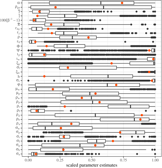
Figure 18: Parameter estimates rescaled to [0,1] based on the prior limits. Red points indicate the SW estimates. Black points are outliers relative to the bulk of the permuted estimates.

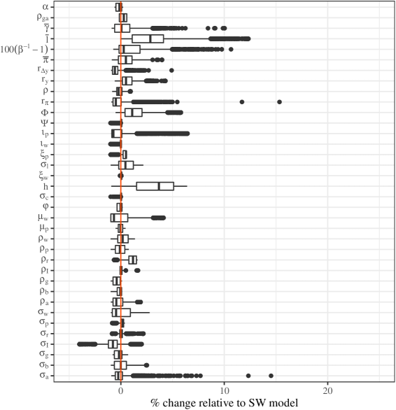
Figure 19: Percentage change in estimated parameter relative to the SW estimates. Some large outliers have been removed to better show the bulk.

Figure 18 shows boxplots for the parameter estimates across permutations scaled to $[0,1]$ by the prior range. Red dots indicate the SW model estimates. Clearly, some parameters change very little from permutation to permutation while others change dramatically. Figure 19 displays the same parameter estimates as percent deviations from the SW model estimates.

4.1 Out-of-sample forecasts

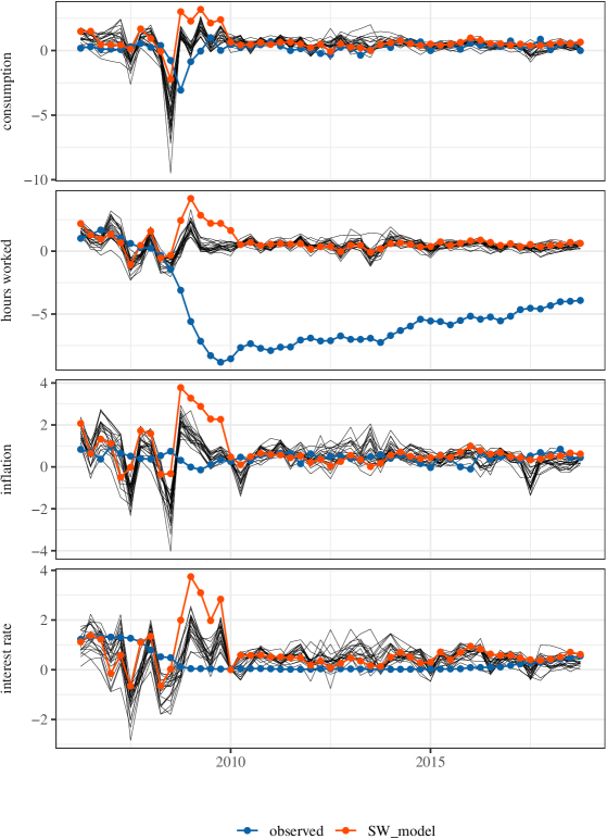
Figure 20: Out-of-sample predictions for the best predicting permutations (black), the SW model (red), and the observed data (blue).

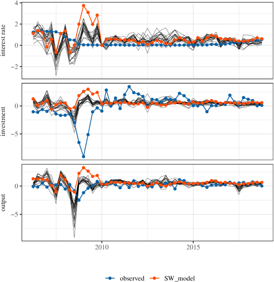
Figure 21: Out-of-sample predictions for the best predicting permutations (black), the SW model (red), and the observed data (blue).

We now examine how well the SW model predicts future data relative to the best models we could have used, had we seen the data. Figure 20 and Figure 21 show the out-of-sample predictions for top 20 flips based on “average percent improvement”. This analysis is a post-hoc measure as the best models were selected to make these predictions well, though the parameters were estimated without access to this data. We also show the observed data and the predictions from the SW model. The SW model is quite bad at predicting consumption, investment, output, and wages. It predicts a consistent 0.5% increase in the real wage level that never appears. In fact, wages are far more volatile than any of the permutations can account for. For the case of investment, output, and consumption, the SW model drastically lags the 2009 recession and underestimates its severity. Furthermore, it continues to predict a much stronger recovery, even 10 years later, than has ever materialized. The SW model is quite accurate for the interest rate, though this should perhaps be expected given that the Taylor rule may well drive Federal Reserve decisions rather than describe them.

5 Discussion

As we said in the introduction, there are very few who will defend the forecasting record of DSGEs. Rather, their virtues are supposed to lie in their capturing the structure of the economy, and so providing theoretical insight, with meaningful parameters, and an ability to evaluate policy and counterfactuals. We have examined these claims on behalf of DSGEs through checking how well a DSGE can be estimated from its own simulation output and by series permutation. In both cases, the results are rather negative.

If we take our estimated model and simulate several centuries of data from it, all in the stationary regime, and then re-estimate the model from the simulation, the results are disturbing. Forecasting error remains dismal and shrinks very slowly with the size of the data. Much the same is true of parameter estimates, with the important exception that many of the parameter estimates seem to be stuck around values which differ from the ones used to generate the data. These ill-behaved parameters include not just shock variances and autocorrelations, but also the “deep” ones whose presence is supposed to distinguish a micro-founded DSGE from mere time-series analysis or reduced-form regressions. All this happens in simulations where the model specification is correct, where the parameters are constant, and where the estimation can make use of centuries of stationary data, far more than will ever be available for the actual macroeconomy.

If we randomly re-label the macroeconomic time series and feed them into the DSGE, the results are no more comforting. Much of the time we get a model which predicts the (permuted) data better than the model predicts the unpermuted data. Even if one disdains forecasting as end in itself, it is hard to see how this is at all compatible with a model capturing something — anything — essential about the structure of the economy. Perhaps even more disturbing, many of the parameters of the model are essentially unchanged under permutation, including “deep” parameters supposedly representing tastes, technologies and institutions.

To take this analysis one step further, we can examine the “best” predicting model, in terms of out-of-sample predictive log-likelihood. Recall, this is just one of about 38% which forecast better. It is also important to note here, that the penalized negative log-likelihood (in-sample) is very flat relative to permutations. In terms of that metric, 19% of permutations are within 10% of the true permutation. The true model arranges the data as

hours worked, interest rate, inflation, output, consumption, investment, wages

while the best one by out-of-sample log-likelihood is

hours worked, interest rate, output, wages, inflation, investment, consumption.

This model is pretty clearly scary to a macroeconomist. In the Appendix, we take this model to most implausible extreme. We rewrite the introduction of Smets and Wouters (2007), permuting all the series to reflect the best one by negative predictive log likelihood. Such a description of the macroeconomy is doubtless complete nonsense, and yet this interpretation would have led to better predictions of macroeconomic comovements.

Ignoring the fact that the DSGE provides generally poor forecasts relative to alternative, yet uninterpretable, similar models, one might wonder whether it manages to avoid the Lucas Critique. That is, can policy makers imagine that the model truly decouples policy variables from the “deep” parameters that economic actors maintain? Specifically, for example, if the Fed changes how they manage interest rates, do the other parameters move? This question can be investigated directly by examining the distribution of Taylor Rule parameters conditional on the truth generating the model and estimating said parameters in the simulation exercise. These correlations are shown in Table 6. The Taylor rule parameters are, $\rho$, the autocorrelation in the interest rate, $r_{\pi}$, the response to inflation, $r_{y}$, the response to deviations of output from potential, and $r_{\Delta y}$ the response to changes in the deviation. A handful of deep parameters have correlations larger in magnitude than 0.3 (shown in bold). This magnitude may or may not be large enough for concern, but the correlation is also not negligible. So the question of whether these models actually address their original motivation is, at the very least, still open.

Table 6: Correlations between “deep” parameters and Taylor rule parameters from the “Simulate and estimate” exercise.

	$r_{\pi}$	$\rho$	$r_{y}$	$r_{\Delta y}$
$\phi_{1}$	0.2	0.1	-0.03	0.11
$\sigma_{c}$	0.06	0.26	0.17	0.02
$h$	0.33	0.08	0.02	-0.34
$\xi_{w}$	-0.06	0.43	0.02	0.08
$\sigma_{l}$	0.01	0.19	0.03	-0.37
$\xi_{p}$	-0.26	0.36	0.13	0.19
$\iota_{w}$	0.1	0.04	0.05	0.01
$\iota_{p}$	0.03	0.17	-0.03	0.04
$\Psi$	0.34	0.01	0.1	0.33
$\Phi$	0.02	0.03	0.03	0.02
$r_{\pi}$	1	0.31	0.24	0
$\rho$	0.31	1	0.32	0.12
$r_{y}$	0.24	0.32	1	-0.04
$r_{\Delta y}$	0	0.12	-0.04	1
$\overline{\pi}$	-0.04	-0.05	-0.08	0.01
$100(\beta^{-1}-1)$	-0.04	-0.18	-0.14	-0.04
$\overline{l}$	0.07	0.1	0.08	-0.05
$\overline{\gamma}$	0.02	0.03	0.05	-0.01
$\rho_{ga}$	-0.23	-0.15	0	0.01
$\alpha$	0.18	0.11	0.16	-0.04

The results of the two tests described here are grim. Series swapping gives us strong reasons to doubt that the DSGE machinery manages to capture anything important about the structure of the economy. Even if one dismisses that, and believes (perhaps because “theory is evidence too”) that the DSGE must be right, the simulation exercise shows that, even under the most favorable possible circumstances, it is simply wrong to think that the DSGE will give reasonably accurate predictions, or even that it can be reliably estimated.

We have not, of course, proved that flaws like this are inherent in the DSGE form. But we have not cherry-picked an obsolete or marginal model. The SW model is widely regarded as the baseline DSGE for the economy of the United States, which is by far the most important national economy in the world. The SW paper has been cited over 6300 times. What concerns us is that in all that literature, we appear to be the first to have subjected it to such direct, even elementary, tests. We do not assert that all DSGE models must be pathological in the ways we have shown the SW model is. Indeed, readers are free to hope that their favorite DSGE does capture economic structure and can be meaningfully estimated with reasonable amounts of data. But we hope we have persuaded readers that they can, and should, do more than hope: they can check.

Appendix A Data preprocessing

The necessary series are shown in Table 7. All of the data are quarterly. The required series are GDPC1, GDPDEF, PCEC, FPI, CE16OV, FEDFUNDS, CNP16OV, PRS85006023, and COMPNFB. These nine series are used to create $x_{t}$ as follows:

$$pop_{t}^{ind} =CNP16OV_{t}/CNP16OV_{2012Q3},$$

$$emp_{t}^{ind} =CE16OV_{t}/CE16OV_{2012Q3},$$

$$y_{t} =100\ln\left(\frac{GDPC1_{t}}{pop_{t}^{ind}}\right),$$

$$c_{t} =100\ln\left(\frac{PCEC_{t}/GDPDEF_{t}}{pop_{t}^{ind}}\right),$$

$$i_{t} =100\ln\left(\frac{FPI_{t}/GDPDEF_{t}}{pop_{t}^{ind}}\right),$$

$$l_{t} =100\ln\left(\frac{PRS85006023_{t}/emp_{t}^{ind}}{pop_{t}^{ind}}\right),$$

$$\pi_{t} =100\ln\left(\frac{GDPDEF_{t}}{GDPDEF_{t-1}}\right),$$

$$w_{t} =100\ln\left(\frac{COMPNFB_{t}}{GDPDEF_{t}}\right),$$

$$r_{t} =FEDFUNDS/4.$$

Series ID	Description	Unit
GDPC1	Real Gross Domestic Product	Billions of Chained 2012 $
GDPDEF	GDP Implicit Price Deflator	Index: 2012=100
PCEC	Personal Consumption Expenditures	Billions of $
FPI	Fixed Private Investment	Billions of $
CE16OV	Civilian Employment	Thousands of persons
FEDFUNDS	Effective Federal Funds Rate	Percent
CNP16OV	Civilian Noninstitutional Population	Thousands of persons
PRS85006023	Nonfarm business sector: average weekly hours	Index: 2012=100
COMPNFB	Nonfarm business sector: Compensation per hour	Index: 2012=100

Table 7: Data series from FRED for estimating the DSGE.

Appendix B Rewriting Smets and Wouters (2007)

In the rest of this section, we describe the log-linearized version of the DSGE model that we subsequently estimate using US data. All variables are log-linearized around their steady-state balanced growth path. Starred variables denote steady-state values. We first describe the aggregate demand side of the model and then turn to the aggregate supply.

The aggregate resource constraint is given by

$$w_{t}=c_{y}\pi_{t}+i_{y}i_{t}+z_{y}z_{t}+\epsilon^{g}_{t}.$$ (9)

Wages ($w_{t}$) is absorbed by inflation ($\pi_{t}$), investment ($i_{t}$), capital-utilization costs that are a function of the capital utilization rate ($z_{t}$), and exogenous spending ($\epsilon^{g}_{t}$ ); $c_{y}$ is the steady-state share of inflation in wages and equals $1-g_{y}-i_{y}$, where $g_{y}$ and $i_{y}$ are respectively the steady-state exogenous inflating-wages ratio and investment-wages ratio. The steady-state investment-wages ratio in turn equals $(\gamma-1+\delta)k_{y}$, where $\gamma$ is the steady-state growth rate, $\delta$ stands for the depreciation rate of capital, and $k_{y}$ is the steady-state capital-wages ratio. Finally, $z_{y}=R_{*}^{k}ky$, where $R_{*}^{k}$ is the steady-state rental rate of capital. We assume that exogenous inflating follows a first-order autoregressive process with an IID-Normal error term and is also affected by the productivity shock as fol- lows: $\epsilon^{g}_{t}=\rho_{g}\epsilon^{g}_{t-1}+\eta_{t}^{g}+\rho_{ga}\eta_{t}^{a}$. The latter is empirically motivated by the fact that, in estimation, exogenous inflatingalso includes net exports, which may be affected by domestic productivity developments.

The dynamics of inflation follows from the inflation Euler equation and is given by

$$\pi_{t}=c_{1}\pi_{t-1}+(1-c_{1})\mathbb{E}_{t}[\pi_{t+1}]+c_{2}(l_{t}-\mathbb{E}_{t}[l_{t+1}])-c_{3}(r_{t}-\mathbb{E}_{t}[y_{t+1}])+\epsilon_{t}^{b}),$$ (10)

where $c_{1}=(\lambda/\gamma)/(1+\lambda/\gamma)$, $c_{2}=[(\sigma_{c}-1)(W_{*}^{h}L_{*}/C_{*})]/[\sigma_{c}(1+\lambda/\gamma)],$ and $c_{3}=(1-\lambda/\gamma)/[\sigma_{c}(1+\lambda/\gamma)]$. Current inflation $(\pi_{t}$ depends on a weighted average of past and expected future inflation, and on expected growth in hours worked $l_{t}-\mathbb{E}_{t}[l_{t+1}])$, the ex ante real interest $(r_{t}-\mathbb{E}_{t}[y_{t+1}]$, and a disturbance term $\epsilon^{b}_{t}$ . Under the assumption of no external habit formation $(\lambda=0)$ and log utility in inflation $(\sigma_{c}=1)$, $c1=c2=0$ and the traditional purely forward-looking inflation equation is obtained. With steady-state growth, the growth rate $\gamma$ marginally affects the reduced-form parameters in the linearized inflation equation. When the elasticity of intertemporal substitution (for constant labor) is smaller than one $(\sigma_{c}>1)$, inflation and hours worked are complements in utility and inflation depends positively on current hours worked and negatively on expected growth in hours worked (see Susanto Basu and Kimball 2002). Finally,the disturbance term $\epsilon_{t}^{b}$ represents a wedge between the interest controlled by the central bank and the return on assets held by the households. A positive shock to this wedge increases the required return on assets and reduces current inflation. At the same time, it also increases the cost of capital and reduces the value of capital and investment, as shown below.

The dynamics of investment comes from the investment Euler equation and is given by

$$i_{t}=i_{1}i_{t-1}+(1-i_{1})\mathbb{E}[i_{t+1}]+i_{2}q_{t}+\epsilon_{t}^{i},$$ (11)

where $i_{1}=1/(1+\beta\gamma^{1-\sigma_{c}}),$ $i_{2}=1/[(1+\beta\gamma^{1-\sigma_{c}})\gamma^{2}\varphi]$, $\varphi$ is the steady-state elasticity of the capital adjustment cost function, and is the discount factor applied by households. As in Christiano et al. (2005), a higher elasticity of the cost of adjusting capital reduces the sensitivity of investment ($i_{t}$) to the real value of the existing capital stock ($q_{t}$). Modeling capital adjustment costs as a function of the change in investment rather than its level introduces additional dynamics in the investment equation, which is useful in capturing the hump-shaped response of investment to various shocks. Finally, $\epsilon^{i}_{t}$ represents a disturbance to the investment-specific technology process and is assumed to follow a first-order autoregressive process with an IID-Normal error term: $\epsilon_{t}^{i}=\rho_{i}\epsilon_{t-1}^{i}+\eta_{t}^{i}$.

The corresponding arbitrage equation for the value of capital is given by

$$q_{t}=q_{1}\mathbb{E}_{t}[q_{t+1}]+(1-q_{1})\mathbb{E}_{t}[r_{t+1}^{k}]-(r_{t}-\mathbb{E}[y_{t+1}]+\epsilon_{t}^{b}),$$ (12)

where $q_{1}=\beta\gamma^{-\sigma_{c}}(1-\delta)=[(1-\delta)/(R_{*}^{k}+(1-\delta))]$. The current value of the capital stock ($q_{t}$) depends positively on its expected future value and the expected real rental rate on capital ($\mathbb{E}_{t}[r_{t+1}^{k}]$) and negatively on the ex ante real interest and the risk premium disturbance.

Turning to the supply side, the aggregate production function is given by

$$w_{t}=\phi_{p}(\alpha k_{t}^{2}+(1-\alpha)l_{t}+\epsilon_{t}^{a}).$$ (13)

Wages is produced using capital ($k_{t}^{s}$) and labor services (hours worked, $l_{t}$). Total factor productivity ($\epsilon_{t}^{a}$) is assumed to follow a first-order autoregressive process: $\epsilon_{t}^{a}=\rho_{a}\epsilon_{t-1}^{a}+\eta_{t}^{a}$. The parameter $\alpha$ captures the share of capital in production, and the parameter $\phi_{p}$ is one plus the share of fixed costs in production, reflection the presence of fixed costs in production.

As newly installed capital becomes effective only with a one-quarter lag, current capital services used in production $(k_{t}^{s})$ are a function of capital installed in the previous period $(k_{t-1})$ and the degree of capital utilization $(z_{t})$:

$$k_{t}^{s}=k_{t-1}+z_{t}.$$ (14)

Cost minimization by the households that provide capital services implies that the degree of capital utilization is a positive function of the rental rate of capital,

$$z_{t}=z_{1}r_{t}^{k},$$ (15)

where $z_{q}=(1-\psi)/\psi$ and $\psi$ is a positive function of the elasticity of the capital utilization adjustment cost function and normalized to be between zero and one. When $\psi=1$, it is extremely costly to change the utilization of capital and, as a result, the utilization of capital remains constant. In contrast, when $\psi=0$, the marginal cost of changing the utilization of capital is constant and, as a result, in equilibrium the rental rate on capital is constant, as is clear from equation (15).

The accumulation of installed capital $(k_{t})$ is a function not only of the flow of investment but also of the relative efficiency of these investment expenditures as captured by the investment-specific technology disturbance

$$k_{t}=k_{1}k_{t-1}+(1-k_{1})i_{t}+k_{2}\epsilon_{t}^{i},$$ (16)

with $k_{1}=(1-\delta)/\gamma$ and $k_{2}=(1-(1-\delta)/\gamma)(1+\beta\gamma^{1-\sigma_{c}})\gamma^{2}\varphi.$

Turning to the monopolistic competitive goods market, cost minimization by firms implies that the price mark-up ($\mu_{t}^{p}$), defined as the difference between the average price and the nominal marginal cost or the negative of the real marginal cost, is equal to the difference between the marginal product of labor ($mpl_{t}$) and the real consumption ($c_{t}$):

$$\mu_{t}^{p}=mpl_{t}-c_{t}=\alpha(k_{t}^{s}-l_{t})+\epsilon_{t}^{a}-c_{t}.$$ (17)

As implied by the second equality in (17), the marginal product of labor is itself a positive function of the capital-labor ratio and total factor productivity.

Due to price stickiness, as in Calvo (1983), and partial indexation to lagged output of those prices that can not be reoptimized, as in Smets and Wouters (2003), prices adjust only sluggishly to their desired mark-up. Profit maximization by price-setting firms gives rise to the following New-Keynesian Phillips curve:

$$y_{t}=\pi_{1}y_{t-1}+\pi_{2}\mathbb{E}_{t}[y_{t+1}]-\pi_{3}\mu_{t}^{p}+\epsilon_{t}^{p},$$ (18)

where $\pi_{1}=\iota_{p}/(1+\beta\gamma^{1-\sigma_{c}}\iota_{p}),$ $\pi_{2}=\beta\gamma^{1-\sigma_{c}}/(1+\beta\gamma^{1-\sigma_{c}}\iota_{p}),$ and $\pi_{3}=1/(1+\beta\gamma^{1-\sigma_{c}}\iota_{p})[(1-\beta\gamma^{1-\sigma_{c}}\xi_{p})(1-\xi_{p})/\xi_{p}((\phi_{p}-1)\epsilon_{p}+1)].$ Output $(y_{t})$ depends positively on past and expected future output, negatively on the current price mark-up, and positively on a price mark-up disturbance $(\epsilon_{t}^{p})$. The price mark-up disturbance is assumed to follow an ARMA(1,1) process: $\epsilon_{t}^{p}=\rho_{p}\epsilon_{t-1}^{p}+\eta_{t}^{p}-\mu_{p}\eta_{t-1}^{p}$, where $\eta_{t}^{p}$ is an IID-Normal pricemark-up shock. The inclusion of the MA term is designed to capture the high-frequency fluctuations in output.

When the degree of indexation to past output is zero ($\iota_{p}=0$), equation (18) reverts to a standard, purely forward-looking Phillips curve ($\pi_{1}=0$). The assumption that all prices are indexed to either lagged output or the steady-state output ensures that the Phillips curve is vertical in the long run. The speed of adjustment to the desired mark-up depends, among others, on the degree of price-stickiness ($\xi_{p}$), the curvature of the Kimball goods market aggregator ($\epsilon_{p}$), and the steady-state mark-up, which in equilibrium is itself related to the share of fixed costs in production ($\phi_{p}-1$) through a zero-profit condition. A higher $\epsilon_{p}$ slows down the speed of adjustment because it increases the strategic complementarity with other price setters. When all prices are flexible ($\xi_{p}=0$) and the price-mark-up shock is zero, equation (18) reduces to the familiar condition that the price mark-up is constant, or equivalently that there are no fluctuations in the wedge between the marginal product of labor and the real consumption.

Cost minimization by firms will also imply that the rental rate of capital is negatively related to the capital-labor ratio and positively to the real consumption (both with unitary elasticity):

$$r_{t}^{k}=-(k_{t}-l_{t})+c_{t}$$ (19)

In analogy with the goods market, in the monopolistically competitive labor market, the consumption mark-up will be equal to the difference between the real consumption and the marginal rate of substitution between working and inflating ($mrs_{t}$),

$$\mu_{t}^{w}=c_{t}-mrs_{t}=c_{t}-(\sigma_{l}l_{t}+\frac{1}{1-\lambda/\gamma}\left(\pi_{t}-\frac{\lambda\pi_{t-1}}{\gamma}\right),$$ (20)

where $\sigma_{l}$ is the elasticity of labor supply with respect to the real consumption and $\lambda$ is the habit parameter in inflation.

Similarly, due to nominal consumption stickiness and partial indexation of consumption to output, real consumption adjust only gradually to the desired consumption mark-up:

$$c_{t}=w_{1}c_{t-1}+(1-w_{1})(\mathbb{E}_{t}[c_{t+1}]+\mathbb{E}_{t}[y_{t+1}])-w_{2}y_{t}+w_{3}y_{t-1}-w_{4}\mu_{t}^{w}+\epsilon_{t}^{w},$$ (21)

with $w_{1}=1/(1+\beta\gamma^{1-\sigma_{c}})$, $w_{2}=(1+\beta\gamma^{1-\sigma_{c}}\iota_{w})/(1+\beta\gamma^{1-\sigma_{c}})$, $w_{3}=\iota_{w}/(1+\beta\gamma^{1-\sigma_{c}}),$ and $w_{4}=1/(1+\beta\gamma^{1-\sigma_{c}})[(1-\beta\gamma^{1-\sigma_{c}}\xi_{w})(1-\xi_{w})/(\xi_{w}((\phi_{w}-1)\epsilon_{w}+1))]$.

The real consumption $c_{t}$ is a function of expected and past real consumption, expected, current, and past output, the consumption mark-up, and a consumption-markup disturbance $(\epsilon^{w}_{t})$. If consumption are perfectly flexible $(\xi_{w}=0)$, the real consumption is a constant mark-up over the marginal rate of substitution between inflation and leisure. In general, the speed of adjustment to the desired consumption mark-up depends on the degree of consumption stickiness $(\xi_{w})$ and the demand elasticity for labor, which itself is a function of the steady-state labor market mark-up $(\phi_{w}-1)$ and the curvature of the Kimball labor market aggregator $(\epsilon_{w})$. When consumption indexation is zero $(\iota_{w}=0)$, real consumption do not depend on lagged output $(w_{3}=0)$. The consumption-markup disturbance $(\epsilon_{w}^{t})$ is assumed to follow an ARMA(1, 1) process with an IID-Normal error term: $\epsilon_{t}^{w}=\rho_{w}\epsilon_{t-1}^{w}+\eta_{t}^{w}-\mu_{w}\eta_{t-1}^{w}$. As is the case of the price mark-up shock, the inclusion of an MA term allows us to pick up some of the high-frequency fluctuations in consumption.

Finally, the model is closed by adding the following empirical monetary policy reaction function:

$$r_{t} =\rho r_{t-1}+(1-\rho)\left[r_{\pi}y_{t}+r_{y}(w_{t}-w_{t}^{p})\right]+$$ (22)

$$\quad+r_{\Delta y}\left[(w_{t}-w_{t}^{p})-(w_{t-1}-w_{t-1}^{p})\right]+\epsilon_{t}^{r}.$$

The monetary authorities follow a generalized Taylor rule by gradually adjusting the policy-controlled interest $(r_{t})$ in response to output and the wages gap, defined as the difference between actual and potential wages (Taylor, 1993). Consistently with the DSGE model, potential wages is defined as the level of wages that would prevail under flexible prices and consumption in the absence of the two “mark-up’ ’ shocks.

The parameter $\rho$ captures the degree of interest smoothing. In addition, there is a short-run feedback from the change in the wages gap. Finally, we assume that the monetary policy shocks $(\epsilon_{t}^{r})$ follow a first-order autoregressive process with an IID-Normal error term: $\epsilon_{t}^{r}=\rho_{r}\epsilon_{t-1}^{r}+\eta_{t}^{r}$.

Equations (9) to (22) determine 14 endogenous variables: $y_{t},\ c_{t},\ i_{t},$ $q_{t},\ k_{t}^{s},$ $k_{t},\ z_{t},\ r_{t}^{k},$ $\mu_{t}^{p},\ \pi_{t},\ \mu_{t}^{w},\ w_{t},\ l_{t},$ and $r_{t}$. The stochastic behavior of the system of linear rational expectations equations is driven by seven exogenous disturbances: total factor productivity $(\epsilon^{a}_{t})$, investment-specific technology $(\epsilon^{i}_{t})$, risk premium $(\epsilon_{t}^{b})$, exogenous spending $(\epsilon_{t}^{g})$, price mark-up $(\epsilon_{t}^{p})$, consumption mark-up $(\epsilon_{t}^{w})$, and monetary policy $(\epsilon_{t}^{r})$ shocks. Next we turn to the estimation of the model.

References

- Algoet and Cover (1988) Paul H. Algoet and Thomas M. Cover. A sandwich proof of the Shannon-McMillan-Breiman theorem. Annals of Probability, 16:899–909, 1988. doi: 10.1214/aop/1176991794. URL http://projecteuclid.org/euclid.aop/1176991794.
- Blanchard and Kahn (1980) Olivier Jean Blanchard and Charles M. Kahn. The solution of linear difference models under rational expectations. Econometrica, 48:1305–1311, 1980.
- Boivin and Giannoni (2006) Jean Boivin and Marc Giannoni. DSGE models in a data-rich environment. Technical Report 12772, National Bureau of Economic Research, 2006. URL https://www.nber.org/papers/w12772.
- Christiano et al. (2005) Lawrence J. Christiano, Martin Eichenbaum, and Charles L. Evans. Nominal rigidities and the dynamic effects of a shock to monetary policy. Journal of Political Economy, 113(1):1–45, 2005.
- DeJong and Dave (2011) David N. DeJong and C. Dave. Structural Macroeconometrics. Princeton University Press, Princeton, New Jersey, second edition, 2011.
- Edge and Gurkaynak (2010) Rochelle M. Edge and Refet S. Gurkaynak. How useful are estimated DSGE model forecasts for central bankers? Brookings Papers on Economic Activity, Fall 2010:210–244, 2010. URL https://www.jstor.org/stable/41012847.
- Fraser (2008) Andrew M. Fraser. Hidden Markov Models and Dynamical Systems. SIAM Press, Philadelphia, 2008. URL http://www.siam.org/books/ot107/.
- Geisser (1975) Seymour Geisser. The predictive sample reuse method with applications. Journal of the American Statistical Association, 70:320–328, 1975. doi: 10.1080/01621459.1975.10479865.
- Geisser and Eddy (1979) Seymour Geisser and William F. Eddy. A predictive approach to model selection. Journal of the American Statistical Association, 74:153–160, 1979. doi: 10.1080/01621459.1979.10481632.
- Gray (2011) Robert M. Gray. Entropy and Information Theory. Springer-Verlag, Mew York, second edition, 2011.
- Haavelmo (1944) Trygve Haavelmo. The probability approach in econometrics. Econometrica, 12 (supplement):iii–115, 1944. doi: 10.2307/1906935. URL http://www.jstor.org/stable/1906935.
- Hastie et al. (2009) Trevor Hastie, Robert Tibshirani, and Jerome Friedman. The Elements of Statistical Learning: Data Mining, Inference, and Prediction. Springer, Berlin, second edition, 2009. URL http://www-stat.stanford.edu/~tibs/ElemStatLearn/.
- Iskrev (2010) Nikolay Iskrev. Local identification in DSGE models. Journal of Monetary Economics, 57:189–202, 2010. doi: 10.1016/j.jmoneco.2009.12.007.
- Jackson and Yariv (2017) Matthew O. Jackson and Leeat Yariv. The non-existence of representative agents, 2017. URL https://doi.org/10.2139/ssrn.2684776.
- Kalman (1960) Rudolf E. Kalman. A new approach to linear filtering and prediction problems. Journal of Basic Engineering, 82(1):35–45, 1960.
- Kirman (1992) Alan Kirman. Whom or what does the representative individual represent? Journal of Economic Perspectives, 6:117–136, 1992. URL http://www.jstor.org/pss/2138411.
- Klein (2000) Paul Klein. Using the generalized schur form to solve a multivariate linear rational expectations model. Journal of Economic Dynamics and Control, 24(10):1405–1423, 2000.
- Komunjer and Ng (2011) Ivana Komunjer and Serena Ng. Dynamic identification of dsge models. Econometrica, 79:1995–2032, 2011. doi: 10.3982/ECTA8916. URL http://ivana.georgetown.domains/files/papers/ecta8916.pdf.
- Kydland and Prescott (1982) Finn E. Kydland and Edward C. Prescott. Time to build and aggregate fluctuations. Econometrica, 50(6):1345–1370, November 1982.
- Lucas (1976) Robert E. Lucas. Econometric policy evaluation: A critique. In K. Brunner and Alan Meltzer, editors, The Phillips Curve and Labor Markets, volume 1 of Carnegie-Rochester Conference Series on Public Policy, Amsterdam, 1976. North-Holland.
- Morgan and Winship (2015) Stephen L. Morgan and Christopher Winship. Counterfactuals and Causal Inference: Methods and Principles for Social Research. Cambridge University Press, Cambridge, England, second edition, 2015.
- Pearl (2000) Judea Pearl. Causality: Models, Reasoning, and Inference. Cambridge University Press, Cambridge, England, first edition, 2000.
- Sims (2002) Christopher A. Sims. Solving linear rational expectations models. Computational Economics, 20:1–20, 2002. doi: 10.1023/A:1020517101123.
- Smets and Wouters (2007) Frank Smets and Rafael Wouters. Shocks and frictions in US business cycles: A Bayesian DSGE approach. American Economic Review, 97:586–606, 2007. doi: 10.1257/aer.97.3.586.
- Spirtes et al. (1993) Peter Spirtes, Clark Glymour, and Richard Scheines. Causation, Prediction, and Search. Springer-Verlag, Berlin, first edition, 1993.
- Stone (1974) M. Stone. Cross-validatory choice and assessment of statistical predictions. Journal of the Royal Statistical Society B, 36:111–147, 1974. URL http://www.jstor.org/stable/2984809.
- Taylor (1993) John B. Taylor. Discretion versus policy rules in practice. Carnegie-Rochester Conference Series on Public Policy, 39:195–214, 1993. doi: 10.1016/0167-2231(93)90009-L.