Is the “RG-invariant EFT” for few-nucleon systems cutoff independent?

Abstract

We consider nucleon-nucleon scattering using the formulation of chiral effective field theory which is claimed to be renormalization group invariant. The cornerstone of this framework is the existence of a well-defined infinite-cutoff limit for the scattering amplitude at each order of the expansion, which should not depend on a particular regulator form. Focusing on the ${}^{3}P_{0}$ partial wave as a representative example, we show that this requirement can in general not be fulfilled beyond the leading order, in spite of the perturbative treatment of subleading contributions to the amplitude. Several previous studies along these lines, including the next-to-leading order calculation by Long and Yang [Phys. Rev. C84, 057001 (2011)] and a toy model example with singular long-range potentials by Long and van Kolck [Annals Phys. 323, 1304-1323 (2008)], are critically reviewed and scrutinized in detail.

I Introduction

The methods of chiral effective field theory (EFT) were first applied to few-nucleon systems in the pioneering work by Weinberg Weinberg (1990, 1991). In the past decades, chiral EFT has established itself as a standard tool in nuclear physics, see Refs. Bedaque and van Kolck (2002); Epelbaum et al. (2009); Machleidt and Entem (2011); Epelbaum and Meißner (2012); Epelbaum et al. (2020a); Hammer et al. (2020) for reviews. One of the key ingredients of the EFT approach in the few-nucleon sector is the resummation of an infinite series of the iterations of (at least) the leading-order (LO) two-nucleon-irreducible terms to account for the non-perturbative nature of the nucleon-nucleon (NN) interaction. Such a non-perturbative resummation requires a regularization of an infinite number of divergent diagrams, which is typically realized by introducing an artificial ultraviolet regulator, a cutoff $\Lambda$. This is particularly relevant for spin-triplet channels of NN scattering, which probe the singular nature of the one-pion-exchange potential. It is commonly agreed that physical observables cannot depend on a particular choice of the cutoff as long as all possible terms in the effective Lagrangian are taken into account. However, the way to implement this requirement in concrete schemes based on some kind of a systematically improvable perturbative expansion is not yet finally settled.

One pragmatic approach relies on using cutoffs of the order of the expected breakdown scale $\Lambda_{b}$ of chiral EFT Lepage (1997); Epelbaum and Meißner (2013). The residual cutoff dependence of the scattering amplitude is expected to become weaker as one increases the EFT order of the calculation. This feature has indeed been verified numerically by explicit calculations, see e.g. Ref. Epelbaum (2016). The finite-cutoff scheme has been pushed to high orders in the EFT expansion, leading to remarkably accurate results, see Refs. Reinert et al. (2018); Entem et al. (2017); Filin et al. (2020); Reinert et al. (2021); Filin et al. (2021) for selected examples. Recently, first steps were made to formally justify this framework by explicitly demonstrating its renormalizability in the EFT sense Gasparyan and Epelbaum (2022a, b).

An alternative approach consists in enforcing cutoff independence of the scattering amplitude at each EFT order separately by taking the limit $\Lambda\to\infty$, i.e. by choosing the cutoff much larger than the EFT breakdown scale $\Lambda_{b}$. In other words, one requires that the amplitude $T^{(n)}$, where $n$ denotes an EFT order, approaches a finite limit

$$T^{(n)}_{\Lambda}\xrightarrow[\Lambda\to\infty]{}T^{(n)}_{\infty},\quad\quad\Lambda\frac{dT^{(n)}_{\Lambda}}{d\Lambda}\xrightarrow[\Lambda\to\infty]{}0.$$ (1)

The amplitude is then claimed to satisfy renormalization group (RG) invariance (RGI). In practical applications of this scheme, a finite cutoff value $\Lambda\gtrsim\Lambda_{b}$ can be employed as long as one can show that the asymptotic behaviour of the amplitude is already reached Hammer et al. (2020). More details on this approach and its applications to few-nucleon systems can be found in recent review articles Hammer et al. (2020); van Kolck (2020).

One of the motivations for such an approach is a quantum mechanical treatment of singular potentials, i.e. potentials that behave at the origin as $r^{-\alpha}$ with $\alpha\geq 2$, see Frank et al. (1971) for a review. Such quantum mechanical problems show similarity to chiral EFT, because the unregulated one-pion-exchange potential in spin-triplet channels behaves at short distances as $1/r^{3}$. It is known that one can obtain a unique solution for the scattering amplitude with such singular potentials by constructing the so-called self-adjoined extension of the Hamiltonian. The solution depends on one arbitrary parameter in each attractive partial wave where the potential is singular, which can be fixed e.g. by using the experimental value of the amplitude at some energy point. In the language of EFT, this corresponds to introducing one contact interaction (a counter term) in each attractive spin-triplet partial wave where the one-pion-exchange potential is treated non-perturbatively. Consequently, the number of counter terms gets “reduced” compared to the perturbative analysis of Feynman diagrams involving multiple iterations of the leading-order potential, from which it follows that an infinite number of counter terms would be necessary in every spin-triplet partial wave.

This scheme has been criticized in Refs Epelbaum and Gegelia (2009); Epelbaum et al. (2018); Epelbaum et al. (2020b); Epelbaum et al. (2021) based on general arguments such as the absence of an explicit transition between the perturbative and non-perturbative regimes, issues with non-perturbative repulsive interactions, appearance of spurious bound states, etc. There are also technical complications that may prevent an application of this scheme to few-nucleon systems, since large cutoff values typically result in high computational cost needed for reaching converged results. For an extensive discussion of these and related issues see Ref. Tews et al. (2022).

Regardless of the above criticism, the infinite-cutoff scheme seems so far yielding reasonable results for NN scattering van Kolck (2020), which is our main focus here. In the context of chiral EFT, the discussed approach was first applied to NN scattering in Ref. Nogga et al. (2005), where the cutoff independence of the LO partial wave amplitudes was demonstrated by a direct numerical calculation.

It is also well established that a consistent inclusion of next-to-leading-order (NLO) interactions within the RG invariant scheme is only possible perturbatively, i.e. using the distorted-wave Born approximation. This is because of a singular behaviour of the NLO potential at short distances, which becomes particularly problematic when it is repulsive, see Refs. Pavon Valderrama and Ruiz Arriola (2006a, b); Zeoli et al. (2013); van Kolck (2020). A perturbative inclusion of the NLO terms in spin-triplet channels within the infinite-cutoff scheme was considered in Refs. Long and Yang (2011, 2012) using a regularization scheme in momentum space, see Refs. Valderrama (2011); Pavon Valderrama (2011) for an analogous approach in coordinate space. A numerical test of the cutoff independence was performed by varying the cutoff up to $\Lambda\simeq 5$ GeV. The number of the NLO counter terms was determined based on the short-range behaviour of the LO wave function and of the NLO potential. Another study in support of the infinite-cutoff scheme was carried out in Ref. Long and van Kolck (2008), where the authors considered a toy model with the LO long-range potential $V_{\text{LO}}\sim 1/r^{2}$ and the NLO long-range potential $V_{\text{NLO}}\sim 1/r^{4}$. This choice of the long-range interactions allows one to perform a part of the analysis analytically. An incomplete proof of the cutoff independence of the NLO amplitude was presented in Ref. Long and van Kolck (2008).

In the present work, we reconsider the infinite-cutoff scheme for NN scattering at NLO in the EFT expansion and critically examine the findings of Refs. Long and Yang (2012, 2011); Long and van Kolck (2008). We demonstrate that the oscillating nature of the LO wave function near the origin caused by the singular (attractive) behavior of the LO potential generally prevents one from achieving a cutoff-independent result for the subleading scattering amplitude in the $\Lambda\to\infty$ limit. To keep our considerations simple we focus here on the case of NN scattering in the ${}^{3}P_{0}$ partial wave, which may serve as a representative example.

Our paper is organized as follows. In Sec. II we illustrate the above-mentioned issue of the infinite-cutoff scheme based on general arguments and using a simplified version of the NN two-pion-exchange potential. In Sec. III we examine in detail the NLO analysis by Long and Yang Long and Yang (2012) and critically revise their conclusions. The implications and generalizations of our results are discussed in Sec. IV. Next, in Sec. V, we consider the toy model example of Ref. Long and van Kolck (2008). The complete renormalizability proofs of the LO and NLO scattering amplitudes for this toy model are given in appendices A and B, respectively. The main results of our paper are summarized in Sec. VI.

II General discussion

In this section we present a general discussion of the issues emerging in the infinite-cutoff scheme at NLO on a rather qualitative and not fully mathematically rigorous level. These considerations are sufficient to illustrate the main idea of our paper. The analytical considerations are supplemented by numerical calculations using the NN two-pion-exchange potential, modified to exhibit a more regular behavior at short distances. This modification allows us to simplify the presentation by reducing the number of subtractions in the NLO amplitude. We focus on NN scattering in the ${}^{3}P_{0}$ partial wave and analyze in detail the cutoff dependence of the amplitude. This partial wave provides as a typical example of the attractive spin-triplet channel, where the one-pion-exchange potential is non-perturbative, and is particularly easy to analyze due to the absence of coupled channels. The results can be generalized to other partial waves in a straightforward way.

II.1 Formalism

We start with describing the formalism. We consider the LO (NLO) potential $V^{\rm\scriptscriptstyle LO{}}$ ($V^{\rm\scriptscriptstyle NLO{}}$) in chiral EFT, with $V^{\rm\scriptscriptstyle LO{}}$ consisting of the one-pion-exchange potential and the short-range part:

$$V^{\rm\scriptscriptstyle LO{}}=V_{1\pi,\Lambda}+V^{\rm\scriptscriptstyle LO{}}_{\text{short},\Lambda},$$ (2)

where the subscript $\Lambda$ signifies that the corresponding potential is regulated. The short-range part $V^{\rm\scriptscriptstyle LO}_{\text{short},\Lambda}$ involves the $S$-wave contact interactions and the counter terms necessary for the renormalization of the LO amplitude, in particular, the leading contact terms in the spin-triplet channels where the one-pion-exchange potential is attractive and treated non-perturbatively. Here and in what follows, we denote by $\Lambda$ the set of all values of cutoffs $\Lambda=\{\Lambda_{i}\}$ that a quantity $X_{\Lambda}$ depends upon. The NLO potential is given by the leading two-pion-exchange potential to be specified below and the short-range part

$$V^{\rm\scriptscriptstyle NLO{}}=V_{2\pi,\Lambda}+V^{\rm\scriptscriptstyle NLO{}}_{\text{short},\Lambda}.$$ (3)

The short-range potentials consist of contact interactions multiplied by the corresponding low-energy constants (LECs),

$$V^{\rm\scriptscriptstyle LO}_{\text{short},\Lambda} =C_{0}V^{\rm\scriptscriptstyle LO}_{\text{ct},0,\Lambda}+\dots,$$

$$V^{\rm\scriptscriptstyle NLO{}}_{\text{short},\Lambda} =\sum_{i=0}^{n}C^{\rm\scriptscriptstyle NLO{}}_{2i}V^{\rm\scriptscriptstyle NLO{}}_{\text{ct},2i,\Lambda}+\dots,$$ (4)

where we only specify explicitly terms contributing to the ${}^{3}P_{0}$ partial wave and omit the channel indices. The second subscript of $V^{\rm\scriptscriptstyle LO}_{\text{ct},0,\Lambda}$ and $V^{\rm\scriptscriptstyle NLO{}}_{\text{ct},2i,\Lambda}$ gives the power of momenta counted relative to the LO contribution, i.e. $V^{\rm\scriptscriptstyle LO}_{\text{ct},0,\Lambda}\sim\vec{p}\,^{2}$ and $V^{\rm\scriptscriptstyle NLO{}}_{\text{ct},2i,\Lambda}\sim\vec{p}\,^{2i+2}$. The upper limit $n$ in the sum over $i$ is determined by the number of counter terms necessary for the renormalization of the NLO amplitude. The explicit form of the short-range potentials will be given below.

Some statements on the regularization are in order here. Since the EFT formulation considered here aims at a complete elimination of regulator dependence van Kolck (2020), the infinite-cutoff limit of the scattering amplitude should not depend on a particular regularization prescription. As stated in Ref. Song et al. (2017), “RGI requires not only independence of observables on the numerical value of the cutoff $\Lambda$ but also independence on the form of the regulator function itself”. Since the potential involves several different structures, one always has a freedom to employ different types of the regulators and cutoff values for each of them.

The regularized potential in the plain-wave basis is obtained from the unregularized one by multiplying it with the corresponding form factor $F_{\Lambda}(\vec{p}\,^{\prime},\vec{p}\,)$. Throughout this work, we will mostly use non-local regulators

$$F_{\Lambda}(\vec{p}\,^{\prime},\vec{p}\,)=F_{\Lambda}(p^{\prime})F_{\Lambda}(p),$$ (5)

where $F_{\Lambda}(p)$ is either the smooth power-like form factor,

$$F_{\Lambda}(p) =\left(\frac{\Lambda^{2}}{\Lambda^{2}+p^{2}}\right)^{n},$$ (6)

with $n$ chosen sufficiently large to remove all divergences, or the sharp cutoff,

$$F_{\Lambda}(\vec{p}\,^{\prime},\vec{p}\,)=\theta(\Lambda-p^{\prime})\theta(\Lambda-p).$$ (7)

The non-local regulators can be applied directly to the partial-wave projected potentials. In Sec. II.4, we will also discuss the case of a locally regularized potential with

$$F_{\Lambda}(\vec{p}\,^{\prime},\vec{p}\,) =\Phi_{\Lambda}(q^{2}),$$ (8)

where $\vec{q}=\vec{p}\,^{\prime}-\vec{p}$ and $\Phi(q^{2})$ is some smooth regulator, e.g.,

$$\Phi_{\Lambda}(q^{2}) =\left(\frac{\Lambda^{2}}{\Lambda^{2}+q^{2}}\right)^{n}.$$ (9)

It will become obvious from our analysis that other forms and types of regulators used in the literature including Gaussian regulators, spectral function regularization or regularizations in coordinate space, which are, to a large extent, equivalent to $q^{2}$-dependent regulators in momentum space, will lead to the same qualitative results.

For simplicity, we will use the same type of the regulator for all parts of the LO and NLO potentials. Moreover, the long-range and short-range parts of the LO potential will be regularized using the same cutoff $\Lambda_{0}$. Similarly, the long-range and the leading short-range parts of the NLO potential will be regularized by the same cutoff $\Lambda_{2}$. Other possible contact terms of the NLO potential are allowed to have independent regulators $\Lambda_{2,i}$ with $i=2,4,\dots$. The sharp cutoffs will be used in Sec. III.

In general, the existence of an infinite-cutoff limit implies that various cutoffs can be taken to infinity independently:

$$\Lambda_{0}(\tau)\xrightarrow[\tau\to\infty]{}\infty,\qquad\Lambda_{2}(\tau)\xrightarrow[\tau\to\infty]{}\infty,\qquad\dots,$$ (10)

where $\Lambda_{0}(\tau)$, $\Lambda_{2}(\tau)$,…are (in general) different functions.

The potential in the ${}^{3}P_{0}$ partial wave is obtained from the potential in the plane wave basis

$$V= V_{C}+V_{\sigma}\vec{\sigma}_{1}\cdot\vec{\sigma}_{2}+V_{\sigma q}\left(\vec{\sigma}_{1}\cdot\vec{q}\,\right)\left(\vec{\sigma}_{2}\cdot\vec{q}\,\right)+V_{SL}i\frac{1}{2}\left(\vec{\sigma}_{1}+\vec{\sigma}_{2}\right)\cdot(\vec{p}\times\vec{p}\,^{\prime})\,,$$ (11)

where we kept only the structures relevant for our calculation, by the projection formula Epelbaum et al. (2000):

$$V(p^{\prime},p)=2\pi\int_{-1}^{1}dz\Big{\{}zV_{C}(\vec{p}\,^{\prime},\vec{p}\,)+zV_{\sigma}(\vec{p}\,^{\prime},\vec{p}\,)-\left[\left(p^{\prime 2}+p^{2}\right)z-2p^{\prime}p\right]V_{\sigma q}(\vec{p}\,^{\prime},\vec{p}\,)+p^{\prime}p(z^{2}-1)V_{SL}(\vec{p}\,^{\prime},\vec{p}\,)\Big{\}}.$$ (12)

The angular integration in Eq. (12) is performed over $z=\cos\theta$, with $\theta$ the angle between the initial and final center-of-mass momenta of the nucleons $\vec{p}$ and $\vec{p}\,^{\prime}$.

The non-vanishing structures of the one-pion- and two-pion-exchange potentials (up to irrelevant polynomial terms) read Kaiser et al. (1997):

$$V_{1\pi,\sigma q}(\vec{p}\,^{\prime},\vec{p}\,)=-\bigg{(}\frac{g_{A}}{2F_{\pi}}\bigg{)}^{2}\frac{1}{q^{2}+M_{\pi}^{2}},$$ (13)

and

$$V_{2\pi,C}(\vec{p}\,^{\prime},\vec{p}\,) =-\frac{L(q)}{384\pi^{2}F_{\pi}^{4}}\biggl{[}4M_{\pi}^{2}(5g_{A}^{4}-4g_{A}^{2}-1)+q^{2}(23g_{A}^{4}-10g_{A}^{2}-1)+\frac{48g_{A}^{4}M_{\pi}^{4}}{4M_{\pi}^{2}+q^{2}}\biggr{]},$$

$$V_{2\pi,\sigma q}(\vec{p}\,^{\prime},\vec{p}\,) =-\frac{1}{q^{2}}V_{2\pi,\sigma}(\vec{p}\,^{\prime},\vec{p}\,)=-\frac{3g_{A}^{4}}{64\pi^{2}F_{\pi}^{4}}L(q),$$ (14)

where

$$L(q)=\frac{1}{q}\sqrt{4M_{\pi}^{2}+q^{2}}\log\frac{\sqrt{4M_{\pi}^{2}+q^{2}}+q}{2M_{\pi}}.$$ (15)

Further, $M_{\pi}$, $F_{\pi}$ and $g_{A}$ refer to the pion mass, decay constant and nucleon axial constant, respectively. For illustrative purposes, we will also consider in Sec. II.3 a simplified version of the two-pion-exchange potential $\tilde{V}_{2\pi}(\vec{p}\,^{\prime},\vec{p}\,)$ by making it less singular at short distances via

$$\tilde{V}_{2\pi}(\vec{p}\,^{\prime},\vec{p}\,) =V_{2\pi}(\vec{p}\,^{\prime},\vec{p}\,)\frac{(3M_{\pi})^{2}}{(3M_{\pi})^{2}+q^{2}},$$ (16)

without modifying the longest-range part of the interaction.

The unregularized contact terms in the ${}^{3}P_{0}$ partial-wave have the form

$$V^{\rm\scriptscriptstyle LO}_{\text{ct},0} =V^{\rm\scriptscriptstyle NLO{}}_{\text{ct},0}=pp^{\prime},$$

$$V^{\rm\scriptscriptstyle NLO{}}_{\text{ct},2} =pp^{\prime}(p^{2}+p^{\prime 2}),\;\dots$$ (17)

When using local regulators, the unregularized ${}^{3}P_{0}$ contact terms can be chosen via

$$V^{\rm\scriptscriptstyle LO}_{\text{ct},0,C} =V^{\rm\scriptscriptstyle LO}_{\text{ct},0,\sigma}=-\frac{1}{32\pi}q^{2},$$

$$V^{\rm\scriptscriptstyle LO}_{\text{ct},0,\sigma q} =-\frac{1}{2}V^{\rm\scriptscriptstyle LO}_{\text{ct},0,SL}=\frac{1}{16\pi},$$ (18)

in order that projections onto other partial waves vanish, see also Ref. Gezerlis et al. (2014). Analogous expressions can be constructed for higher-order contact interactions.

The LO amplitude $T^{\rm\scriptscriptstyle LO}$ is obtained by solving the Lippmann-Schwinger equation

$$T^{\rm\scriptscriptstyle LO}=V^{\rm\scriptscriptstyle LO}+V^{\rm\scriptscriptstyle LO}GT^{\rm\scriptscriptstyle LO},$$ (19)

or more explicitly,

$$T^{\rm\scriptscriptstyle LO}(p^{\prime},p;p_{\text{on}}) =V^{\rm\scriptscriptstyle LO}(p^{\prime},p)+\int\frac{p^{\prime\prime 2}dp^{\prime\prime}}{(2\pi)^{3}}V^{\rm\scriptscriptstyle LO}(p^{\prime},p^{\prime\prime})G(p^{\prime\prime};p_{\text{on}})T^{\rm\scriptscriptstyle LO}(p^{\prime\prime},p;p_{\text{on}}),$$

$$G(p^{\prime\prime};p_{\text{on}}) =\frac{m_{N}}{p_{\text{on}}^{2}-p^{\prime\prime 2}+i\epsilon},$$ (20)

where $p_{\text{on}}$ denotes the on-shell center-of-mass momentum and $m_{N}$ is the nucleon mass. The NLO amplitude is given by the distorted-wave Born approximation

$$T^{\rm\scriptscriptstyle NLO{}}=(\mathds{1}+T^{\rm\scriptscriptstyle LO}G)V^{\rm\scriptscriptstyle NLO{}}(\mathds{1}+GT^{\rm\scriptscriptstyle LO}).$$ (21)

We can also define separately $T_{2\pi}$ and $T_{\text{ct},i}$,

$$T_{2\pi} =(\mathds{1}+T^{\rm\scriptscriptstyle LO}G)V_{2\pi,\Lambda}(\mathds{1}+GT^{\rm\scriptscriptstyle LO}),$$

$$T_{\text{ct},i} =(\mathds{1}+T^{\rm\scriptscriptstyle LO}G)V^{\rm\scriptscriptstyle NLO{}}_{\text{ct},i,\Lambda}(\mathds{1}+GT^{\rm\scriptscriptstyle LO}),\qquad i=0,2,\dots,$$ (22)

so that the full NLO amplitude is given by

$$T^{\rm\scriptscriptstyle NLO{}}=T_{2\pi}+\sum_{i=0}^{n}C^{\rm\scriptscriptstyle NLO{}}_{2i}T_{\text{ct},2i}.$$ (23)

Notice further that the amplitude $T^{\rm\scriptscriptstyle LO}$ depends on the cutoff $\Lambda_{0}$ alone, while the amplitude $T^{\rm\scriptscriptstyle NLO{}}$ is a function of all cutoffs $\Lambda$, which we do not always indicate explicitly.

II.2 Dispersive approach

As already mentioned in Sec. I, the LO amplitude $T^{\rm\scriptscriptstyle LO}$ is required to have an infinite-cutoff limit in the “RG-invariant” EFT scheme, see Eq. (1). Therefore, we assume that by choosing an appropriate renormalization condition for the constant $C_{0}=C_{0}(\Lambda_{0})$, one obtains a finite limit for the on-shell ($p^{\prime}=p=p_{\text{on}}$) LO amplitude:

$$T^{\rm\scriptscriptstyle LO}_{\Lambda}(p_{\text{on}})=T^{\rm\scriptscriptstyle LO}_{\infty}(p_{\text{on}})\{1+O[\left(\bar{q}/\Lambda_{0}\right)^{\alpha_{0}}]\},$$ (24)

where $\bar{q}=\max(p_{\text{on}},M_{\pi})$ and $\alpha_{0}$ is some positive number. This follows from the general theory of singular potentials Frank et al. (1971) and is supported by the numerical calculations performed in Ref. Nogga et al. (2005). Analogously, the phase shift $\delta^{\rm\scriptscriptstyle LO}(p_{\text{on}})$ approaches its limiting value at $\Lambda_{0}\to\infty$ for a given finite value of $p_{\text{on}}$ when using the normalization $\delta(0)=0$ in order to avoid the shifts generated by deeply bound states.

As the renormalization condition, we are free to fix e.g. the scattering volume or the value of the phase shift at any energy point $p_{0}$, $|p_{0}|\ll\Lambda_{0}$, above or below threshold:

$$\delta^{\rm\scriptscriptstyle LO}(p_{0})=\delta^{\rm\scriptscriptstyle LO}_{0}.$$ (25)

It is common to choose $\delta^{\rm\scriptscriptstyle LO}_{0}$ equal to the empirical phase shift extracted from experimental data:

$$\delta^{\rm\scriptscriptstyle LO}_{0}=\delta_{\text{exp}}(p_{0}).$$ (26)

In the considerations below we assume that we can regard both $V^{\rm\scriptscriptstyle LO}$ and $V^{\rm\scriptscriptstyle NLO{}}$ as being local. Strictly speaking, this is only the case if the regulators of the LO and NLO potentials are local. If the regulators are non-local, one can still expect our arguments to apply, because the non-localities appear at momenta $p\sim\Lambda$ and should only induce corrections vanishing in the $\Lambda\to\infty$ limit, which are allowed in the resulting formulas in any case. Since the potentials are assumed to be local, one can use an $N/D$ representation for the amplitude $T^{\rm\scriptscriptstyle LO}$ Newton (1982)

$$T^{\rm\scriptscriptstyle LO}(p_{\text{on}})=\frac{p_{\text{on}}^{2}\tilde{N}^{\rm\scriptscriptstyle LO}(p_{\text{on}})}{\tilde{D}(p_{\text{on}})},$$ (27)

where $\tilde{D}(p_{\text{on}})$ is the Fredholm determinant (equal to the Jost function) and contains all right-hand singularities and bound-state poles of $T^{\rm\scriptscriptstyle LO}$. It can be represented by means of the dispersion relation Newton (1982)

$$\tilde{D}(p_{\text{on}})=\Bigg{(}\prod_{j=1}^{n}\frac{p_{\text{on}}^{2}+\kappa_{j}^{2}}{p_{\text{on}}^{2}}\Bigg{)}\exp\bigg{[}\frac{1}{\pi}\int_{0}^{\infty}dp^{2}\frac{\tilde{\delta}^{\rm\scriptscriptstyle LO}(p)}{p_{\text{on}}^{2}-p^{2}+i\epsilon}\bigg{]},$$ (28)

where $n$ denotes the number of bound states and $p_{j}=i\kappa_{j}$ are the positions of the bound-state poles. The factor $p_{\text{on}}^{2}$ in front of $\tilde{N}^{\rm\scriptscriptstyle LO}$ in Eq. (27) reflects the orbital angular momentum $l=1$. In Eq. (28), $\tilde{\delta}^{\rm\scriptscriptstyle LO}(p)$ is the LO phase shift normalized to $\tilde{\delta}^{\rm\scriptscriptstyle LO}(\infty)=0$. In our case, it is more suitable to use an alternative representation with a subtraction at $p_{\text{on}}=0$ in terms of $\delta^{\rm\scriptscriptstyle LO}(p)$:

$$D(p_{\text{on}})=\Bigg{(}\prod_{j=1}^{n}\frac{p_{\text{on}}^{2}+\kappa_{j}^{2}}{\kappa_{j}^{2}}\Bigg{)}\exp\left[\frac{1}{\pi}\int_{0}^{\infty}dp^{2}\frac{p_{\text{on}}^{2}}{p^{2}}\frac{\delta^{\rm\scriptscriptstyle LO}(p)}{p_{\text{on}}^{2}-p^{2}+i\epsilon}\right],$$ (29)

so that

$$T^{\rm\scriptscriptstyle LO}(p_{\text{on}})=\frac{p_{\text{on}}^{2}N^{\rm\scriptscriptstyle LO}(p_{\text{on}})}{D(p_{\text{on}})},$$ (30)

where $N^{\rm\scriptscriptstyle LO}(p_{\text{on}})$ contains only left-hand singularities. Under the reasonable assumption that the integral in Eq. (29) converges at momenta $p\ll\Lambda_{0}$, and provided the bound states lie far away from the threshold, we can conclude that $D(p_{\text{on}})$ also approaches a finite limit as $\Lambda_{0}\to\infty$:

$$D_{\Lambda_{0}}(p_{\text{on}})=D_{\infty}(p_{\text{on}})\{1+O[\left(\bar{q}/\Lambda_{0}\right)^{\alpha_{D}}]\},\qquad\alpha_{D}>0.$$ (31)

The $N/D$ representation for the subleading amplitudes $T_{2\pi}$ and $T_{\text{ct},i}$ reads

$$T_{2\pi}(p_{\text{on}}) =\frac{p_{\text{on}}^{2}N_{2\pi}(p_{\text{on}})}{D(p_{\text{on}})^{2}},$$

$$T_{\text{ct},i}(p_{\text{on}}) =\frac{p_{\text{on}}^{2}N_{\text{ct},i}(p_{\text{on}})}{D(p_{\text{on}})^{2}}.$$ (32)

Again, the functions $N_{2\pi}(p_{\text{on}})$ and $N_{\text{ct},i}(p_{\text{on}})$ possess only left-hand singularities. If we further assume that both the LO and the NLO potentials are of Yukawa type, which is true for the regulators of the form given in Eq. (9), the location of the left-hand singularities and their properties are well known Martin (1961), and we can write down the corresponding dispersion relations

$$N_{2\pi}(p_{\text{on}}) =\int_{-\infty}^{-M_{\pi}^{2}}\frac{dp^{2}}{\pi}\frac{\Delta N_{2\pi}(p)}{p^{2}-p_{\text{on}}^{2}},$$

$$N_{\text{ct},i}(p_{\text{on}}) =\int_{-\infty}^{-\Lambda_{2,i}^{2}/4}\frac{dp^{2}}{\pi}\frac{\Delta N_{\text{ct},i}(p)}{p^{2}-p_{\text{on}}^{2}},\qquad\Lambda_{2,0}\equiv\Lambda_{2}.$$ (33)

The discontinuity $\Delta N_{2\pi}(p)$ in the region $-\Lambda_{\text{min}}^{2}/4<p^{2}<-M_{\pi}^{2}$, where $\Lambda_{\text{min}}=\min(\Lambda)$, is determined by the perturbative contributions such as $V^{\rm\scriptscriptstyle NLO{}}$, $V^{\rm\scriptscriptstyle NLO{}}GV^{\rm\scriptscriptstyle LO}$, etc., and is independent of $\Lambda$. Therefore, we can expect the following $\Lambda$-behaviour of $N_{2\pi}$ and $N_{\text{ct},i}$:

$$N_{2\pi,{\Lambda}}(p_{\text{on}}) =N_{2\pi,\infty}(p_{\text{on}})+P_{2\pi,{\Lambda}}(p_{\text{on}}^{2})+O[\left(\bar{q}/\Lambda\right)^{\alpha_{2\pi}}],$$

$$N_{\text{ct},i,{\Lambda}}(p_{\text{on}}) =P_{\text{ct},i,{\Lambda}}(p_{\text{on}}^{2})+O[\left(\bar{q}/\Lambda\right)^{\alpha_{\text{ct}}}],\qquad\alpha_{2\pi},\alpha_{\text{ct}}>0,$$ (34)

where $P_{2\pi,{\Lambda}}(p_{\text{on}}^{2})$ and $P_{\text{ct},i,{\Lambda}}(p_{\text{on}}^{2})$ are polynomials in $p_{\text{on}}^{2}$, which may contain positive powers of $\Lambda$, and $\bar{q}/\Lambda$ denotes $\bar{q}/\Lambda_{\text{min}}$. Their degrees correspond to the number of subtractions necessary to suppress the momentum region $p\sim\Lambda$ in dispersive integrals in Eq. (33).

Now, let us first assume that a single subtraction is sufficient, i.e., both polynomials $P_{2\pi,{\Lambda}}(p_{\text{on}}^{2})$ and $P_{\text{ct},i,{\Lambda}}(p_{\text{on}}^{2})$ are simply $\Lambda$-dependent constants,

$$P_{2\pi,{\Lambda}}(p_{\text{on}}^{2})\equiv C_{2\pi}({\Lambda}),\quad\quad P_{\text{ct},0,{\Lambda}}(p_{\text{on}}^{2})\equiv C_{\text{ct}}({\Lambda}),$$ (35)

and

$$C^{\rm\scriptscriptstyle NLO{}}_{i}=0,\text{ for }i\neq 0.$$ (36)

This situation describes the case when a more regular version of the two-pion-exchange potential defined in Eq. (16) is used. We will study such a simplified model numerically in the next subsection.

Combining the estimates in Eqs. (31) and (34) we obtain the following expression for the NLO amplitude:

$$T^{\rm\scriptscriptstyle NLO{}}_{{\Lambda}}(p_{\text{on}}) =\frac{p_{\text{on}}^{2}}{D_{\infty}(p_{\text{on}})^{2}}\Big{\{}N_{2\pi,\infty}(p_{\text{on}})+C_{2\pi}({\Lambda})+C^{\rm\scriptscriptstyle NLO{}}_{0}({\Lambda})\left[C_{\text{ct}}({\Lambda})+\delta N_{\text{ct},{\Lambda}}(p_{\text{on}})\right]+\delta N_{2\pi,{\Lambda}}(p_{\text{on}})\Big{\}},$$

$$\delta N_{2\pi,{\Lambda}}(p_{\text{on}}) =O[\left(\bar{q}/\Lambda\right)^{\alpha}],$$

$$\delta N_{\text{ct},{\Lambda}}(p_{\text{on}}) =O[\left(\bar{q}/\Lambda\right)^{\beta}],$$ (37)

with $\alpha,\beta>0$. We can now fix the constant $C^{\rm\scriptscriptstyle NLO{}}_{0}({\Lambda})$ by choosing some renormalization condition. If the LO amplitude is fixed by the requirement to reproduce the experimental value at $p_{\text{on}}=p_{0}$, the natural choice is to set

$$T^{\rm\scriptscriptstyle NLO{}}(p_{0})=0.$$ (38)

Then, if one can neglect $\delta N_{\text{ct},{\Lambda}}$ and $\delta N_{2\pi,{\Lambda}}$, the solution to Eq. (38) is

$$C^{\rm\scriptscriptstyle NLO{}}_{0}({\Lambda})=-\frac{N_{2\pi,\infty}(p_{0})+C_{2\pi}({\Lambda})}{C_{\text{ct}}({\Lambda})},$$ (39)

and the NLO amplitude indeed becomes $\Lambda$-independent as $\Lambda$ tends to infinity:

$$T^{\rm\scriptscriptstyle NLO{}}_{{\Lambda}}(p_{\text{on}}) \approx\frac{p_{\text{on}}^{2}}{D_{\infty}(p_{\text{on}})^{2}}\Big{[}N_{2\pi,\infty}(p_{\text{on}})-N_{2\pi,\infty}(p_{0})\Big{]}.$$ (40)

However, the term involving $\delta N_{\text{ct},{\Lambda}}$ can not always be neglected since it is multiplied by $C^{\rm\scriptscriptstyle NLO{}}_{0}({\Lambda})$ which, in general, is unbounded as follows from Eq. (39). As follows from the definition of $T_{\text{ct},0}$ in Eq. (22), the constant $C_{\text{ct}}({\Lambda})$ can be viewed as being proportional to the square of the LO scattering wave function, smeared with some weight over the short distance region $r\sim 1/\Lambda_{2}$, where it strongly oscillates as $\Lambda_{0}$ increases. Therefore, for some values of $\Lambda_{0}$ and $\Lambda_{2}$, $C_{\text{ct}}({\Lambda})$ can become very small, and Eq. (39) must be replaced with

$$C^{\rm\scriptscriptstyle NLO{}}_{0}({\Lambda})=-\frac{N_{2\pi,\infty}(p_{0})+C_{2\pi}({\Lambda})}{C_{\text{ct}}({\Lambda})+\delta N_{\text{ct},{\Lambda}}(p_{0})}.$$ (41)

As one can see, if for some “exceptional” value $\Lambda=\bar{\Lambda}$, one has

$$C_{\text{ct}}({\bar{\Lambda}})+\delta N_{\text{ct},{\bar{\Lambda}}}(p_{0})=0,$$ (42)

while

$$C_{\text{ct}}({\bar{\Lambda}})+\delta N_{\text{ct},{\bar{\Lambda}}}(p_{\text{on}})\not\equiv 0,$$ (43)

i.e., if the zero is not factorizable, then the cutoff independence of $T^{\rm\scriptscriptstyle NLO{}}$ in the vicinity of $\bar{\Lambda}$ and therefore also in general may become questionable. If the constant $C^{\rm\scriptscriptstyle NLO{}}_{0}({\Lambda})$ behaves near the pole $\Lambda=\bar{\Lambda}$ as

$$C^{\rm\scriptscriptstyle NLO{}}_{0}({\Lambda})\approx\bar{C}^{\rm\scriptscriptstyle NLO{}}_{0}(\bar{\Lambda})(\Lambda-\bar{\Lambda})^{-\bar{\alpha}},$$ (44)

where typically $\bar{\alpha}=1$ or $\bar{\alpha}=2$, see the next sections, then, as follows from Eq. (37), the width $\delta\Lambda$ of the “exceptional” regions is roughly of order

$$\delta\Lambda\sim\frac{\bar{C}^{\rm\scriptscriptstyle NLO{}}_{0}(\bar{\Lambda})^{1/\bar{\alpha}}}{\bar{\Lambda}^{\beta/\bar{\alpha}}},$$ (45)

and generally decreases with $\Lambda$ remaining, nevertheless, finite. In the next two subsections we will see how this situation actually occurs in the case of non-locally and locally regulated potentials.

The above discussion was merely meant to identify the “exceptional” values of the cutoffs that may destroy the cutoff independence of the amplitude. In the case of a single subtraction, the relation in Eq. (41) is equivalent to

$$T^{\rm\scriptscriptstyle NLO{}}_{\text{ct},0,\bar{\Lambda}}(p_{0})=0,\quad\quad T^{\rm\scriptscriptstyle NLO{}}_{\text{ct},0,\bar{\Lambda}}(p_{\text{on}})\not\equiv 0.$$ (46)

If more than one, say $n_{\text{sub}}$, subtractions (NLO counter terms) are necessary, we will need additional renormalization conditions to fix the corresponding LECs. It is convenient to define a function $\delta^{\rm\scriptscriptstyle NLO{}}(p_{\text{on}})$,

$$T^{\rm\scriptscriptstyle NLO{}}(p_{\text{on}})=-\delta^{\rm\scriptscriptstyle NLO{}}(p_{\text{on}})\,e^{2i\delta^{\rm\scriptscriptstyle LO}(p_{\text{on}})}\rho(p_{\text{on}}),$$ (47)

with the phase space factor

$$\rho(p_{\text{on}})=\frac{m_{N}}{(2\pi)^{3}}\frac{\pi p_{\text{on}}}{2}.$$ (48)

Analogously, we define the functions $\delta_{2\pi}(p_{\text{on}})$ and $\delta_{\text{ct},i}(p_{\text{on}})$:

$$T_{2\pi}(p_{\text{on}}) =-\delta_{2\pi}(p_{\text{on}})\,e^{2i\delta^{\rm\scriptscriptstyle LO}(p_{\text{on}})}\rho(p_{\text{on}}),$$

$$T_{\text{ct},i}(p_{\text{on}}) =-\delta_{\text{ct},i}(p_{\text{on}})\,e^{2i\delta^{\rm\scriptscriptstyle LO}(p_{\text{on}})}\rho(p_{\text{on}}),\qquad i=0,2,\dots,2(n_{\text{sub}}-1).$$ (49)

The functions $\delta^{\rm\scriptscriptstyle NLO{}}(p_{\text{on}})$, $\delta_{2\pi}(p_{\text{on}})$ and $\delta_{\text{ct},i}(p_{\text{on}})$ are real-valued in the elastic physical region due to the unitarity of the $S$-matrix. They can be identified with the perturbative NLO correction to the phase shift as done e.g. in Ref. Long and Yang (2011). One can impose the following renormalization conditions:

$$\delta^{\rm\scriptscriptstyle NLO{}}(p_{i})=\delta^{\rm\scriptscriptstyle NLO{}}_{i},\qquad i=0,\,2,\,\dots,\,2(n_{\text{sub}}-1),$$ (50)

where $p_{0}$ can be chosen to be the same on-shell momentum as used in the renormalization of the LO amplitude. Alternatively, one can use derivatives of $\delta^{\rm\scriptscriptstyle NLO{}}(p_{\text{on}})$ with respect to $p_{\text{on}}^{2}$ at threshold or impose other conditions. In turn, one can use the empirical phase shifts and set

$$\delta^{\rm\scriptscriptstyle NLO{}}_{i}=\delta_{\text{exp}}(p_{i})-\delta^{\rm\scriptscriptstyle LO}(p_{i}),$$ (51)

which yields $\delta^{\rm\scriptscriptstyle NLO{}}_{0}=0$ if the condition (26) is used. By analogy with Eq. (46), we can easily identify the “exceptional” cutoff values $\bar{\Lambda}$ lying on the trajectories $\Lambda(\tau)$ defined in Eq. (10) that may destroy the cutoff independence of the NLO amplitude via

$$\det A_{\bar{\Lambda}}=0,\quad\quad\det\tilde{A}_{\bar{\Lambda}}\neq 0,$$ (52)

with ($\Lambda$ dependence being omitted)

$$A_{ij}=\delta_{\text{ct},i}(p_{j}),\qquad\tilde{A}_{ij}=\delta_{\text{ct},i}(\tilde{p}_{j}),\qquad i,j=0,\,2,\,\dots,\,2(n_{\text{sub}}-1),$$ (53)

where at least for one $j$, $\tilde{p}_{j}\neq p_{j}$. In what follows, we will present numerical evidence that such “exceptional” cutoff values cannot be avoided in general. The case of a single subtraction will be considered in Sec. II.3, while the case of two subtractions will be discussed in Sec. III.

In all calculations presented below, the following numerical values for the physical constants are employed: the pion decay constant is set to $F_{\pi}=92.1$ MeV, the isospin average nucleon and pion masses are $m_{N}=938.9$ MeV and $M_{\pi}=138.04$ MeV, respectively, and the effective axial coupling constant of the nucleon is set to $g_{A}=1.29$ to account for the Goldberger-Treiman discrepancy, see e.g. Refs. Epelbaum et al. (2005); Fettes et al. (1998). The calculations have been performed using Mathematica Wolfram Research, Inc. .

II.3 Simplified model with a non-local regulator

In this subsection we consider the simplified model for the ${}^{3}P_{0}$ channel using a modified $2\pi$-exchange introduced in Sec. II.1 with the non-local regulator at LO and NLO, see Eq. (5). In this scheme only one subtraction at NLO is needed. We fix the constants $C^{\rm\scriptscriptstyle LO}_{0}$ and $C^{\rm\scriptscriptstyle NLO{}}_{0}$ by the renormalization conditions

$$\delta^{\rm\scriptscriptstyle LO}(p_{0})=\delta_{\text{exp}}(p_{0}),\qquad\delta^{\rm\scriptscriptstyle NLO{}}(p_{0})=0,$$ (54)

where the on-shell momentum $p_{0}$ is chosen to correspond to the laboratory energy of $T_{\text{lab}}=50$ MeV.

The contact part of the on-shell NLO amplitude (Eq. (22)) takes the particularly simple form

$$T_{\text{ct}}(p_{\text{on}}) =C^{\rm\scriptscriptstyle NLO{}}_{0}T_{\text{ct},0}(p_{\text{on}})=C^{\rm\scriptscriptstyle NLO{}}_{0}\psi_{\Lambda}(p_{\text{on}})^{2},$$ (55)

with the vertex function

$$\psi_{\Lambda}(p_{\text{on}})=p_{\text{on}}F_{\Lambda_{2}}(p_{\text{on}})+\int\frac{p^{2}dp}{(2\pi)^{3}}p\,F_{\Lambda_{2}}(p)\,G(p;p_{\text{on}})\,T^{\rm\scriptscriptstyle LO}_{\Lambda_{0}}(p,p_{\text{on}};p_{\text{on}}).$$ (56)

Therefore, the $\Lambda$-independence of the NLO amplitude can be potentially destroyed if

$$\psi_{\Lambda}(p_{0})=0$$ (57)

for some values of $\Lambda_{0}$ and $\Lambda_{2}$.

We start with considering a special case with the LO and NLO cutoffs being set to the same values, $\Lambda_{2}=\Lambda_{0}$, and show that under this condition, the zero of $\psi_{\Lambda}(p_{\text{on}})$ is factorizable. One can demonstrate this using the two-potential formalism. The off-shell LO amplitude is represented as

$$T^{\rm\scriptscriptstyle LO}_{\Lambda_{0}}(p^{\prime},p;p_{\text{on}})=T_{1\pi,\Lambda_{0}}(p^{\prime},p;p_{\text{on}})+\frac{\psi_{1\pi,\Lambda_{0}}(p^{\prime};p_{\text{on}})\,\psi_{1\pi,\Lambda_{0}}(p;p_{\text{on}})}{C_{0}^{-1}-\Sigma_{\Lambda_{0}}(p_{\text{on}})},$$ (58)

where

$$\psi_{1\pi,\Lambda_{0}}(p;p_{\text{on}}) =pF_{\Lambda_{0}}(p)+\int\frac{p^{\prime 2}dp^{\prime}}{(2\pi)^{3}}p^{\prime}\,F_{\Lambda_{0}}(p^{\prime})\,G(p^{\prime};p_{\text{on}})\,T_{1\pi,\Lambda_{0}}(p^{\prime},p;p_{\text{on}}),$$

$$\Sigma_{\Lambda_{0}}(p_{\text{on}}) =\int\frac{p^{2}dp}{(2\pi)^{3}}p\,F_{\Lambda_{0}}(p)G(p;p_{\text{on}})\psi_{1\pi,\Lambda_{0}}(p;p_{\text{on}}).$$ (59)

The $T$-matrix $T_{1\pi}$ is the solution of the LO Lippmann-Schwinger equation without the contact term:

$$T_{1\pi}=V_{1\pi}+V_{1\pi}GT_{1\pi}.$$ (60)

It is straightforward to see that

$$\psi_{\Lambda_{0}}(p_{\text{on}})=\frac{\psi_{1\pi,\Lambda_{0}}(p_{\text{on}})}{1-C_{0}\Sigma_{\Lambda_{0}}(p_{\text{on}})},$$ (61)

where $\psi_{1\pi,\Lambda_{0}}(p_{\text{on}})\coloneqq\psi_{1\pi,\Lambda_{0}}(p_{\text{on}};p_{\text{on}})$.

Numerical checks show that the condition $\psi_{1\pi,\Lambda_{0}}(p_{\text{on}})=0$ is never fulfilled in the physical region. Therefore, $\psi_{\Lambda_{0}}(p_{\text{on}})$ vanishes only when $C_{0}=\infty$. This happens for the “exceptional” values of $\Lambda_{0}=\bar{\Lambda}_{i}$, $i=1,2,\dots$, due to the limit-cycle-like behaviour of $C_{0}(\Lambda_{0})$, see, e.g. Ref. Nogga et al. (2005). In this case, $\psi_{\Lambda_{0}}(p_{\text{on}})$ vanishes identically for all energies as

$$\psi_{\Lambda_{0}}(p_{\text{on}})\sim(\Lambda_{0}-\bar{\Lambda}_{i})\xi_{\bar{\Lambda}_{i}}(p_{\text{on}}).$$ (62)

Then, the constant $C^{\rm\scriptscriptstyle NLO{}}_{0}$ in the vicinity of $\bar{\Lambda}_{i}$ behaves as

$$C^{\rm\scriptscriptstyle NLO{}}_{0}\sim(\Lambda_{0}-\bar{\Lambda}_{i})^{-2},$$ (63)

canceling the overall prefactor $(\Lambda_{0}-\bar{\Lambda}_{i})^{2}$ in $T_{\text{ct}}$, and no problems due to an enhancement of $1/\Lambda^{\beta}$-terms (see the discussion in the previous subsection and Eq. (37)) occur.

The phase shifts corresponding to this solution for a sufficiently large cutoff are shown in the left panel of Fig. 1.

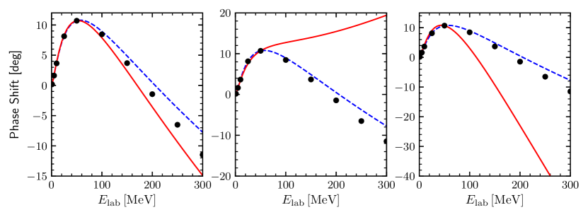
Figure 1: Nucleon-nucleon phase shifts for the ${}^{3}P_{0}$ partial wave versus the laboratory energy calculated using the simplified model with a modified two-pion-exchange potential from Eq. (16). Dashed and solid lines denote the LO and NLO results, respectively. Solid dots are the empirical phase shifts from the Nijmegen partial wave analysis Stoks et al. (1993). The left panel corresponds to a typical value of the cutoff, whereas the other two panels show the phase shifts for the cutoff values near the “exceptional” ones as described in the text. Plots are created using Matplotlib Hunter (2007).

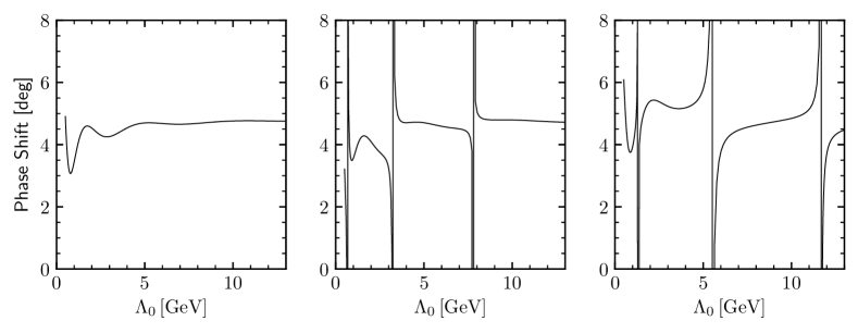
Figure 2: The ${}^{3}P_{0}$ phase shift at the fixed laboratory energy of $T_{\text{lab}}=130$ MeV calculated in the simplified model at NLO as a function of the cutoff for $\Lambda_{2}=\Lambda_{0}$ (left panel), $\Lambda_{2}=2\Lambda_{0}$ (middle panel) and $\Lambda_{2}=\Lambda_{0}/2$ (right panel).

In the left panel of Fig. 2, the NLO result for the phase shift $\delta^{\rm\scriptscriptstyle LO}+\delta^{\rm\scriptscriptstyle NLO{}}$, where $\delta^{\rm\scriptscriptstyle NLO{}}$ is defined according to Eq. (47), is shown as a function of the cutoff at the laboratory energy $T_{\text{lab}}=130$ MeV. One indeed observes the cutoff-independent result as $\Lambda\to\infty$. The situation changes, however, if one sets $\Lambda_{2}\neq\Lambda_{0}$. Below, we consider two cases of a linear dependence of $\Lambda_{2}$ on $\Lambda_{0}$, $\Lambda_{2}=2\Lambda_{0}$ and $\Lambda_{2}=\Lambda_{0}/2$, which reflect a typical situation for any other kind of such a dependence.

Figure 3 shows the locations of zeros of the magnitude of the vertex function $\tilde{\psi}_{\Lambda}(p_{\text{on}})$, defined as

$$\psi_{\Lambda}(p_{\text{on}})=\tilde{\psi}_{\Lambda}(p_{\text{on}})\,e^{i\delta^{\rm\scriptscriptstyle LO}}.$$ (64)

These zeros extend to $\Lambda=\infty$ and for $\Lambda_{2}\neq\Lambda_{0}$ correspond to “exceptional” values of the cutoff. The middle and right panels of Fig. 2 demonstrate that the NLO phase shifts reveal a behaviour far from being constant in the vicinity of the “exceptional” cutoffs. The cutoff dependence of the phase shift is more complicated than just a double pole. In the case of $\Lambda_{2}=2\Lambda_{0}$ ($\Lambda_{2}=\Lambda_{0}/2$) slightly above (below) the pole, there is a point with $\psi_{\Lambda}(p_{\text{on}})=0$ (where $p_{\text{on}}\neq p_{0}$ corresponds to the considered $T_{\text{lab}}=130$ MeV). At this point the NLO amplitude is given completely by the two-pion-exchange term, which leads to another (finite) oscillation of the phase shift in the positive direction. This is a characteristic feature of the scheme with one subtraction.

In Fig. 1, we show how the phase shifts deviate from the solution for the typical cutoff, plotted in the left panel, for the “exceptional” cutoff value $\bar{\Lambda}_{0}=19660.9$ MeV using $\Lambda_{2}=\Lambda_{0}/2$: the middle (right) panel corresponds to the choice $\Lambda_{0}=\bar{\Lambda}_{0}-5$ MeV ($\Lambda_{0}=\bar{\Lambda}_{0}+5$ MeV).

Note that the first “exceptional” cutoff values appear at $\Lambda_{0}\sim 700-1300$ MeV, i.e. for $\Lambda_{0}$ of the order of or slightly above the hard scale $\Lambda_{b}$. This does not automatically imply that a reasonable description of the data is impossible for such cutoff values. For $\Lambda_{0}\sim\Lambda_{b}$, the numerical value of the amplitude $T_{2\pi}$ is rather small in line with expectations based on naive dimensional analysis. Therefore, one could replace the renormalization condition (54), which is the main source of the problem, by the condition

$$\delta^{\rm\scriptscriptstyle LO}(p_{0})+\delta^{\rm\scriptscriptstyle NLO}(p_{0}) =\delta_{\text{exp}}(p_{0}),$$

$$C^{\rm\scriptscriptstyle NLO{}}_{0} =0.$$ (65)

However, in doing so, one unavoidably violates one of the basic principles of the infinite-cutoff scheme stating that the cutoff independence must be achieved at each order individually. Obviously, the condition (65) cannot be adopted for $\Lambda\gg\Lambda_{b}$, because in that case the two-pion-exchange amplitude would violate the dimensional power counting if no subtractions are performed. We do not claim though that no alternative renormalization schemes can be defined, which would employ renormalization conditions different from those in Eq. (54), yet approaching them in the limit $\Lambda\to\infty$ with no “exceptional” cutoffs. However, in such a scheme, the renormalization condition for the LO amplitude would depend on a choice of the regulator of both the LO and the NLO potentials, which seems to make no sense from the physical point of view.

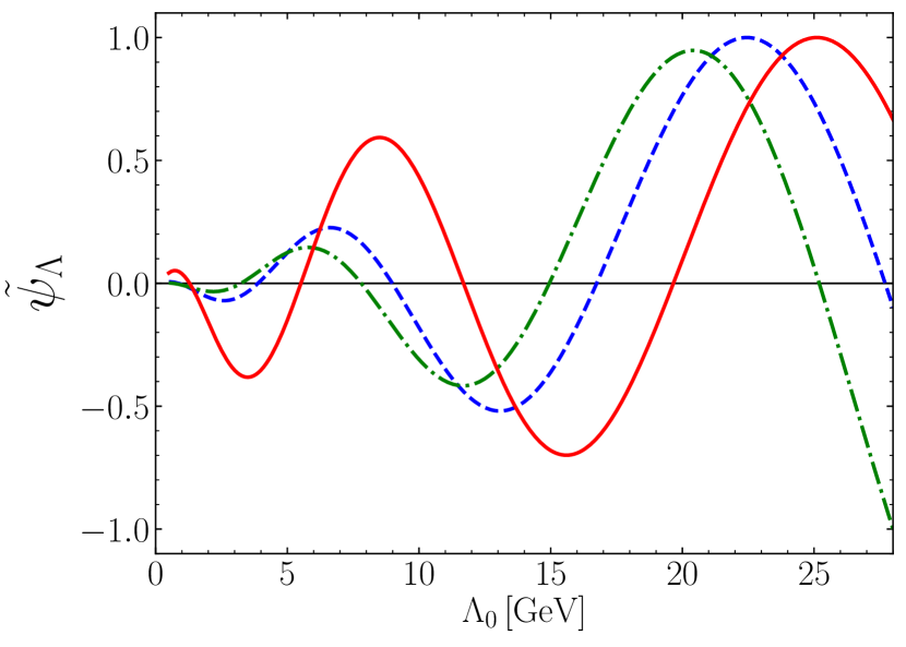
Figure 3: The magnitude of the vertex function $\tilde{\psi}_{\Lambda}(p_{\text{on}})$ defined in Eq. (64) for the simplified model at $p_{\text{on}}=p_{0}$. Dashed, dash-dotted and solid lines correspond to the choice $\Lambda_{2}=\Lambda_{0}$, $\Lambda_{2}=2\Lambda_{0}$ and $\Lambda_{2}=\Lambda_{0}/2$, respectively.

A comment is in order here regarding the choice $\Lambda_{2}=\Lambda_{0}$ discussed above, which prevents the appearance of “exceptional” cutoff values for the considered interactions. One might try to argue that this is a “natural” choice, since the LO contact term and the $p^{\prime}p$ NLO contact terms are parts of the same term in the effective Lagrangian that is split between two orders. However, insisting on such a choice contradicts the principle of the infinite-cutoff scheme that the limit $\Lambda\to\infty$ should not depend on the functional form of the regulator. Note that in the limit $\Lambda\to\infty$, the two contact interactions indeed become identical independently of the relationship between $\Lambda_{0}$ and $\Lambda_{2}$. Moreover, this argument loses its justification completely when additional contact interactions at NLO are included, as there is no physical reason to relate the regulators of such contact terms with the leading-order one. One can in this case not even unambiguously define, what the notion of the same regulator actually means due to a different short-range structure of the contact interactions. In particular, choosing the same sharp cutoff in momentum space still leads to the appearance of “exceptional” values, as we will see in Sec. III. The only possibility to avoid the “exceptional” values as far as we can see is to allow for energy-dependent contact terms of the form $pp^{\prime}p_{\text{on}}^{2i}$, $i=0,1,\dots$ only and to employ a unified form factor in momentum space. But as already argued above, there is no physical motivation for such a prescription.

Given the freedom to choose different regulators for different contact interactions, it is reasonable to expect that performing more than one subtraction at NLO, i.e. adding more contact terms, will not qualitatively change the situation. Since cutoffs for different contact terms are independent, there will (most probably) exist “exceptional” combinations of them, which would prevent the existence of a $\Lambda\to\infty$ limit for the amplitude. The analysis of Sec. III offers an example of such a situation for the case of two NLO contact terms.

II.4 The case of a local regulator

For the sake of completeness, we also briefly comment on the case when all regulators are chosen to be local as done e.g. in Refs. Gezerlis et al. (2013, 2014); Piarulli et al. (2016); Piarulli and Tews (2020); Piarulli and Schiavilla (2021) (of course, we could also use a combination of local and non-local regulators which, however, would not lead to any new conclusions). In this case, the problem of regularization can be equivalently formulated in coordinate space Valderrama (2011); Pavon Valderrama (2011). We adopt the same renormalization conditions as in the previous subsection, which are specified in Eq. (54), and consider again the situation when one subtraction is sufficient to regularize the NLO amplitude, i.e. the model with a modified $2\pi$-exchange potential defined in Sec. II.1.

There is a subtlety appearing already at leading order. In contrast to the previously analyzed case of the non-local regulator, the solution for the LO constant $C_{0}(\Lambda_{0})$ determined by the renormalization condition (54) becomes not unique and depends on the number of spurious bound states, see e.g. Refs. Beane et al. (2001); Bawin and Coon (2003); Braaten and Phillips (2004), leading to different branches of the function $C_{0}(\Lambda_{0})$. Although the description of the ${}^{3}P_{0}$ partial wave does not depend on a choice of a particular branch, one cannot choose $C_{0}(\Lambda_{0})$ too large because this would affect other partial waves, in which the $C_{0}(\Lambda_{0})$ contributions are otherwise suppressed by inverse powers of $\Lambda_{0}$. To compensate for this effect, one would have to introduce additional contact interactions in the affected partial waves.

The NLO amplitude can be conveniently evaluated in $r$-space:

$$T^{\rm\scriptscriptstyle NLO{}}(p_{\text{on}})=\int r^{2}dr\psi_{p_{\text{on}}}^{\rm\scriptscriptstyle LO}(r)^{2}V^{\rm\scriptscriptstyle NLO{}}(r)=e^{2i\delta^{\rm\scriptscriptstyle LO}(p_{\text{on}})}\int r^{2}dr|\psi_{p_{\text{on}}}^{\rm\scriptscriptstyle LO}(r)|^{2}V^{\rm\scriptscriptstyle NLO{}}(r),$$ (66)

where $\psi_{p_{\text{on}}}^{\rm\scriptscriptstyle LO}(r)$ is the LO scattering wave function. Analogously, the contact part of the NLO amplitude is given by

$$T_{\text{ct},0}(p_{\text{on}})=e^{2i\delta^{\rm\scriptscriptstyle LO}(p_{\text{on}})}\int r^{2}dr|\psi_{p_{\text{on}}}^{\rm\scriptscriptstyle LO}(r)|^{2}V^{\rm\scriptscriptstyle NLO{}}_{\text{ct},0,\Lambda_{2}}(r).$$ (67)

One can see that the appearance of “exceptional” cutoffs corresponding to the condition $T_{\text{ct},0}(p_{\text{on}})=0$ can be avoided independently of the behaviour of the LO wave function if the regulated contact NLO potential does not change its sign. Obviously, this condition cannot be fulfilled in general. For example, for the NLO contact interaction in the form of Eq. (18) with the regulator $\Phi_{\Lambda_{2}}(q^{2})$ employed universally for all four structures, one can show that the coordinate-space contact potential has the form (valid only for the ${}^{3}P_{0}$ partial wave)

$$V^{\rm\scriptscriptstyle NLO{}}_{\text{ct},0,{\Lambda_{2}}}(r)={\frac{1}{8\pi}}\bigg{[}\partial^{2}_{r}\Phi_{\Lambda_{2}}(r)-\frac{2}{r}\partial_{r}\Phi_{\Lambda_{2}}(r)\bigg{]},$$ (68)

with

$$\Phi_{\Lambda_{2}}(r) =\int\frac{d^{3}q}{(2\pi)^{3}}\Phi_{\Lambda_{2}}(q^{2})e^{i\vec{q}\cdot\vec{r}}.$$ (69)

For the power-like regulators of Eq. (9) with $n=2$ and $n=3$, we obtain

$$V^{\rm\scriptscriptstyle NLO{}}_{\text{ct},0,\Lambda_{2}}(r) =\frac{\Lambda_{2}^{4}}{64\pi^{2}}(2+\Lambda_{2}r)\frac{e^{-\Lambda_{2}r}}{r},\qquad n=2,$$

$$V^{\rm\scriptscriptstyle NLO{}}_{\text{ct},0,\Lambda_{2}}(r) =\frac{\Lambda_{2}^{5}}{256\pi^{2}}(1+\Lambda_{2}r)e^{-\Lambda_{2}r},\qquad n=3.$$ (70)

For the Gaussian regulator $\Phi_{\Lambda_{2}}(q^{2})=e^{-q^{2}/\Lambda_{2}^{2}}$, the corresponding short-range interaction is given by

$$V^{\rm\scriptscriptstyle NLO{}}_{\text{ct},0,\Lambda_{2}}(r) =\frac{\Lambda_{2}^{5}}{4\pi^{5/2}}\big{(}2+\Lambda_{2}^{2}r^{2}\big{)}e^{-\Lambda_{2}^{2}r^{2}}.$$ (71)

None of the above terms changes its sign. On the other hand, for the regulator in $r$-space in the form $\Phi_{\Lambda_{2}}(r)=\Lambda_{2}^{3}/[\pi\Gamma(3/4)]e^{-\Lambda_{2}^{4}r^{4}}$ adopted in Ref. Gezerlis et al. (2014), we obtain

$$V^{\rm\scriptscriptstyle NLO{}}_{\text{ct},0,\Lambda_{2}}(r) =\frac{\Lambda_{2}^{7}}{2\pi^{2}\Gamma(3/4)}r^{2}\big{(}4\Lambda_{2}^{4}r^{4}-1\big{)}e^{-\Lambda_{2}^{4}r^{4}}.$$ (72)

The latter contact interaction changes its sign at short distances, so that one can tune the LO regulator $\Lambda_{0}$ to make the integral in Eq. (67) vanish. One will also obtain an oscillating behaviour of $V^{\rm\scriptscriptstyle NLO{}}_{\text{ct},0,\Lambda_{2}}(r)$ if one chooses different cutoff values for different structures in Eq. (11) or if one takes a linear combination of the above regulators.

We refrain from providing any numerical results here, which would essentially duplicate the ones from the previous subsection. Nevertheless, we have verified explicitly the existence of “exceptional” cutoffs for the following choice of the regulator:

$$\Phi_{\Lambda_{2}}(q^{2})=2\left(\frac{\Lambda^{2}}{\Lambda^{2}+q^{2}}\right)^{2}-\left(\frac{\Lambda^{2}}{\Lambda^{2}+q^{2}}\right)^{3}.$$ (73)

Note that similarly to our comment on the LO interaction, the constant $C^{\rm\scriptscriptstyle NLO{}}_{0}(\Lambda)$, being infinite for the “exceptional” cutoffs, affects also other partial waves even though such contributions are suppressed by inverse powers of $\Lambda$.

If one includes more than one contact term at NLO, the conclusion about the existence of “exceptional” cutoffs remains the same since such terms are even more oscillating at short distances, so that the condition in Eq. (52) is likely to be satisfied for certain values of $\Lambda$.

There is a particular choice of $\Lambda_{2}$ that ensures the absence of “exceptional” cutoff values, namely $\Lambda_{2}\gg\Lambda_{0}$. In this case, the integral in Eq. (67) is dominated by the region $r\sim 1/\Lambda_{2}$, where the LO wave function is not oscillating anymore and approaches its short-range limit (for the $P$-wave) Newton (1982):

$$\psi_{p_{\text{on}}}^{\rm\scriptscriptstyle LO}(r)\sim\frac{p_{\text{on}}r}{f(p_{\text{on}})}.$$ (74)

Here, $f(p_{\text{on}})$ is the reduced Jost function, which is finite at $p_{\text{on}}=0$. Since the $P$-wave contact interaction behaves effectively as

$$V^{\rm\scriptscriptstyle NLO{}}_{\text{ct},0,\Lambda_{2}\to\infty}(r)\sim\partial^{2}_{r}\delta(\vec{r}\,)$$ (75)

for $\Lambda_{2}\to\infty$, the contact term in Eq. (67) becomes

$$T_{\text{ct},0}(p_{\text{on}})/p_{\text{on}}^{2}\sim\frac{1}{f(p_{\text{on}})^{2}}\neq 0,$$ (76)

and the condition for “exceptional” cutoffs is never fulfilled. The condition $\Lambda_{2}\gg\Lambda_{0}$ is quite different from the constraint $\Lambda_{2}=\Lambda_{0}$ for the absence of “exceptional” cutoffs in the case of non-local regulators, see Sec. II.3. This indicates, once again, that conditions of this kind have no physical origin.

To summarize, we have argued in this section that the two basic principles of the infinite-cutoff scheme or, equivalently, the “RG-invariant” EFT framework stating that

• the amplitude has a well defined $\Lambda\to\infty$ limit at each EFT order and

• this limit does not depend on a particular way it is approached, i.e. on the functional form of the regulators and/or on the relationship among cutoff values at various orders

are in conflict with one another. In general, there is an infinite number of unbounded “exceptional” values of the cutoff, which makes it impossible to formulate a strict infinite-cutoff limit. We have not proved this rigorously, but we have found several “exceptional” cutoffs numerically in each considered case (apart from some very specific choices of regulators) for rather large cutoff values.

III The approach of Long and Yang

We are now in the position to examine the results of Ref. Long and Yang (2011) for the ${}^{3}P_{0}$ NN partial wave at NLO of chiral EFT with respect to the issues discussed above. We do not consider the part of Ref. Long and Yang (2011) devoted to the N²LO amplitude, which would lead to essentially the same conclusions. The scheme of Ref. Long and Yang (2011) is very similar to the simplified model with a non-local regulator considered in Sec. II.3. However, the two-pion-exchange potential is taken in its full form given in Eq. (14), which requires two subtractions at NLO. The NLO potential is then given by

$$V^{\rm\scriptscriptstyle NLO{}}(p^{\prime},p)=V_{2\pi,\Lambda}(p^{\prime},p)+p^{\prime}p\left[C^{\rm\scriptscriptstyle NLO{}}_{0}+C^{\rm\scriptscriptstyle NLO{}}_{2}(p^{\prime 2}+p^{2})\right]F_{\Lambda}(p^{\prime})F_{\Lambda}(p).$$ (77)

Following Ref. Long and Yang (2011), we implement the sharp cutoff instead of a smooth non-local regulator,

$$F_{\Lambda}(p)=\theta(\Lambda-p),$$ (78)

with $\Lambda_{0}=\Lambda_{2}=\Lambda$, which makes no conceptual difference to the choices considered before (even though one would hardly use a sharp cutoff in realistic EFT calculations).

The contact parts of the on-shell NLO amplitude can be represented as follows:

$$T_{\text{ct}}(p_{\text{on}}) =C^{\rm\scriptscriptstyle NLO{}}_{0}T_{\text{ct},0}(p_{\text{on}})+C^{\rm\scriptscriptstyle NLO{}}_{2}T_{\text{ct},2}(p_{\text{on}}),$$

$$T_{\text{ct},0}(p_{\text{on}}) =\psi_{\Lambda}(p_{\text{on}})^{2},$$

$$T_{\text{ct},2}(p_{\text{on}}) =2\psi_{\Lambda}(p_{\text{on}})\psi^{\prime}_{\Lambda}(p_{\text{on}}),$$ (79)

with

$$\psi_{\Lambda}(p_{\text{on}}) =p_{\text{on}}+\int_{0}^{\Lambda}\frac{p^{2}dp}{(2\pi)^{3}}pG(p;p_{\text{on}})T^{\rm\scriptscriptstyle LO}_{\Lambda}(p,p_{\text{on}};p_{\text{on}}),$$

$$\psi^{\prime}_{\Lambda}(p_{\text{on}}) =p_{\text{on}}^{3}+\int_{0}^{\Lambda}\frac{p^{2}dp}{(2\pi)^{3}}p^{3}G(p;p_{\text{on}})T^{\rm\scriptscriptstyle LO}_{\Lambda}(p,p_{\text{on}};p_{\text{on}}).$$ (80)

The authors of Ref. Long and Yang (2011) adopted the following renormalization conditions to fix the constants $C^{\rm\scriptscriptstyle LO}_{0}$, $C^{\rm\scriptscriptstyle NLO{}}_{0}$ and $C^{\rm\scriptscriptstyle NLO{}}_{2}$:

$$\delta^{\rm\scriptscriptstyle LO}(p_{0}) =\delta_{\text{exp}}(p_{0}),$$

$$\delta^{\rm\scriptscriptstyle NLO{}}(p_{0}) =0,$$

$$\delta^{\rm\scriptscriptstyle NLO{}}(p_{1}) =\delta_{\text{exp}}(p_{1})-\delta^{\rm\scriptscriptstyle LO}(p_{1}),$$ (81)

where the on-shell momentum $p_{0}$ ($p_{1}$) was chosen to correspond to the laboratory energy of $T_{\text{lab}}=50$ MeV ($T_{\text{lab}}=25$ MeV). Using the unitarization prescription in Eqs. (47) and (49) we obtain the system of linear equations:

$$\left\{\begin{array}[]{ll}C^{\rm\scriptscriptstyle NLO{}}_{0}\delta_{\text{ct},0}(p_{0})+C^{\rm\scriptscriptstyle NLO{}}_{2}\delta_{\text{ct},2}(p_{0})&=-\delta_{2\pi}(p_{0}),\\ C^{\rm\scriptscriptstyle NLO{}}_{0}\delta_{\text{ct},0}(p_{1})+C^{\rm\scriptscriptstyle NLO{}}_{2}\delta_{\text{ct},2}(p_{1})&=\delta_{\text{exp}}(p_{1})-\delta^{\rm\scriptscriptstyle LO}(p_{1})-\delta_{2\pi}(p_{1}).\end{array}\right.$$ (84)

We can express $\delta_{\text{ct},0}$ and $\delta_{\text{ct},2}$ in terms of the magnitudes of the vertex functions $\tilde{\psi}$ and $\tilde{\psi}^{\prime}$,

$$\psi_{\Lambda}(p_{\text{on}}) =\tilde{\psi}_{\Lambda}(p_{\text{on}})e^{i\delta^{\rm\scriptscriptstyle LO}(p_{\text{on}})},$$

$$\psi_{\Lambda}^{\prime}(p_{\text{on}}) =\tilde{\psi}_{\Lambda}^{\prime}(p_{\text{on}})e^{i\delta^{\rm\scriptscriptstyle LO}(p_{\text{on}})},$$ (85)

as follows:

$$\delta_{\text{ct},0}(p_{\text{on}}) =-\tilde{\psi}_{\Lambda}(p_{\text{on}})^{2}/\rho(p_{\text{on}}),$$

$$\delta_{\text{ct},2}(p_{\text{on}}) =-2\tilde{\psi}_{\Lambda}(p_{\text{on}})\tilde{\psi}_{\Lambda}^{\prime}(p_{\text{on}})/\rho(p_{\text{on}}).$$ (86)

Then, the condition for an “exceptional” cutoff in Eq. (52) becomes

$$\det A_{\bar{\Lambda}}=2\frac{\tilde{\psi}_{\bar{\Lambda}}(p_{0})\tilde{\psi}_{\bar{\Lambda}}(p_{1})}{\rho(p_{0})\rho(p_{1})}\left|\begin{array}[]{ll}\tilde{\psi}_{\bar{\Lambda}}(p_{0})&\tilde{\psi}^{\prime}_{\bar{\Lambda}}(p_{0})\\ \tilde{\psi}_{\bar{\Lambda}}(p_{1})&\tilde{\psi}^{\prime}_{\bar{\Lambda}}(p_{1})\end{array}\right|=0.$$ (89)

As shown in Sec. II.3, the zeros of $\tilde{\psi}_{\Lambda}(p_{0})$ are factorizable, so that $\tilde{\psi}_{\Lambda}(p_{0})=0$ implies $\tilde{\psi}_{\Lambda}(p_{1})=0$. To exclude these zeros from the determinant in Eq. (89) we introduce the following auxiliary quantity:

$$\zeta_{\Lambda}(p_{0},p_{1})=\frac{1}{\tilde{\psi}_{\Lambda}(p_{0})}\left|\begin{array}[]{ll}\tilde{\psi}_{\Lambda}(p_{0})&\tilde{\psi}_{\Lambda}^{\prime}(p_{0})\\ \tilde{\psi}_{\Lambda}(p_{1})&\tilde{\psi}^{\prime}_{\Lambda}(p_{1})\end{array}\right|,$$ (92)

whose zeros determine the genuine “exceptional” cutoffs $\bar{\Lambda}$:

$$\zeta_{\bar{\Lambda}}(p_{0},p_{1})=0.$$ (93)

The quantity $\zeta_{\Lambda}(p_{0},p_{1})$ and the magnitude of the vertex function $\tilde{\psi}_{\Lambda}(p_{0})$ are shown in Fig. 4 as functions of the cutoff $\Lambda$. They are normalized at the maximal points. The zeros of $\zeta_{\Lambda}(p_{0},p_{1})$ are not factorizable, i.e. their positions depend on $p_{0}$ and $p_{1}$, and their locations (including the lowest ones) do not coincide with the zeros of $\tilde{\psi}_{\Lambda}(p_{0})$. Therefore, these zeros indeed correspond to the “exceptional” cutoff values. Notice that the difference in the positions of zeros of $\zeta_{\Lambda}(p_{0},p_{1})$ and $\tilde{\psi}_{\Lambda}(p_{0})$ is an indication of the fact that the expected connection between “exceptional” cutoffs and spurious bound states is not direct: the “exceptional” cutoffs appear at smaller values of $\Lambda$ than the spurious deeply bound states.

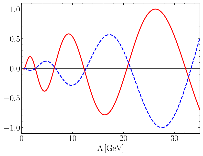
Figure 4: $\Lambda$ dependence of the magnitude of the vertex function (dashed line) $\tilde{\psi}_{\Lambda}(p_{0})$ and of the quantity $\zeta_{\Lambda}(p_{0},p_{1})$ (solid line) for the interaction of Ref. Long and Yang (2011) normalized to their maximal (in absolute value) values.

In the left panel of Fig. 5, we plot the ${}^{3}P_{0}$ phase shift calculated at NLO at $T_{\text{lab}}=130$ MeV as a function of the cutoff $\Lambda$. The curve looks very similar to the one shown in Ref. Long and Yang (2011) and seems to flatten out as $\Lambda$ tends to infinity. The only differences to the plots in Ref. Long and Yang (2011) are the almost vertical lines located at the “exceptional” values of the cutoff.

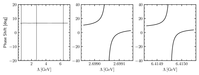
Figure 5: Cutoff dependence of ${}^{3}P_{0}$ phase shift calculated at the fixed laboratory energy of $T_{\text{lab}}=130$ MeV using the approach of Ref. Long and Yang (2011) at NLO. The middle and right panels show zoomed regions in the vicinity of two “exceptional” cutoffs.

The middle and right panels of Fig. 5 demonstrate the behaviour of the phase shift around two “exceptional” points in more detail. As one can see, the width of such “exceptional” regions is of order $0.1$ MeV, which is much smaller than in the case of the simplified model with one subtraction considered in Sec. II.3. The reason for this is obviously the fact that two subtractions performed at NLO lead to a higher power $\beta$ of the residual cutoff dependence in Eq. (37). In Ref. Long and Yang (2011), an estimate $\beta=5/2$ was given based on the short-range behaviour of the LO wave function. Another factor that makes the “exceptional” regions narrower is that the zeros of $\zeta_{\bar{\Lambda}}(p_{0},p_{1})$ are first order, see Eq. (45).

The difference between the behaviour of the phase shifts for the typical and “exceptional” values of the cutoff is illustrated in Fig. 6. The left panel shows the solution for a typical cutoff ($\Lambda=12.5$ GeV), whereas the middle and the right panels correspond to cutoff values slightly below ($\Lambda=12249.69$ MeV) and above ($\Lambda=12249.73$ MeV) an “exceptional” point. This results demonstrate that the NLO phase shifts show essentially arbitrary behavior for cutoffs in the vicinity of the “exceptional” values, which signals the breakdown of the renormalization program.

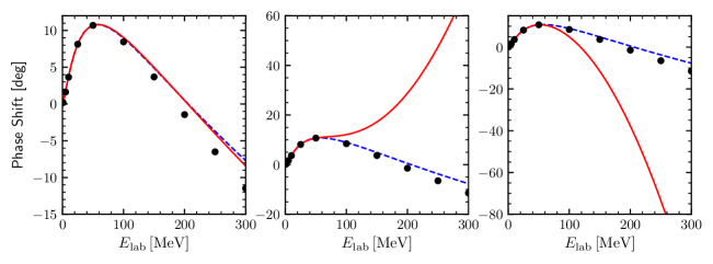
Figure 6: The ${}^{3}P_{0}$ phase shifts calculated using the approach of Ref. Long and Yang (2011) at LO (dashed lines) and NLO (solid lines). The left panel shows the solution for a typical cutoff ($\Lambda=12.5$ GeV), whereas the middle and right panels correspond to the cutoff values slightly below ($\Lambda=12249.69$ MeV) and above ($\Lambda=12249.73$ MeV) the second “exceptional” point.

It is important to keep in mind that the appearance of an infinite number of “exceptional” cutoffs does not depend on the choice of renormalization conditions, which only determine the particular locations of such cutoffs. Moreover, adding further counter terms and fixing them using additional renormalization conditions would not qualitatively change the situation because Eq. (52) would still have solutions, albeit the width of “exceptional” regions would further decrease.

To summarize, the results presented above confirm the analysis based on the simplified model of Sec. II.3. The realistic calculation for the NN system indicates the absence of a definite limit of the NLO amplitude for $\Lambda\to\infty$. We have also highlighted the danger of missing the “exceptional” cutoff regions when numerically verifying the cutoff independence of an amplitude, since their width may be very small.

IV Generalizations

We are now in the position to discuss various straightforward generalizations of the results obtained in Secs. II and III. Since the existence of “exceptional” cutoffs originates from the oscillating nature of the high-momentum part of the $T$-matrix for singular potentials, such cutoffs are expected to generally appear in any infinite-cutoff scheme with the non-perturbative LO attractive singular potential and perturbative inclusion of the NLO corrections. This implies, in particular, that the renormalizability in the sense of the “RG-invariant” EFT framework breaks down in all spin-triplet channels where the one-pion-exchange potential is attractive and needs to be treated non-perturbatively.

Moreover, the obtained results do not qualitatively depend on the long-range part of the LO potential. In particular, we have verified that the “exceptional” cutoffs exist also in the case when the one-pion-exchange potential is taken in the chiral limit with $M_{\pi}=0$, as suggested in Ref. Beane et al. (2002).

It is easy to check that “exceptional” cutoffs appear also in systems where the LO interaction is less singular, e.g. where the LO potential at short distances behaves as $1/r^{2}$ and is sufficiently attractive (one exception being the model of Long and van Kolck Long and van Kolck (2008), which will be discussed in Sec. V). The issues raised in our paper are therefore also relevant for studies of three-body systems with zero-range interactions, such as e.g. three-nucleon scattering in the doublet $S$-wave channel treated within pionless EFT Bedaque et al. (2000) or three-boson systems with large scattering lengths Bedaque et al. (1999). In those cases, the leading-order interaction with an infinite cutoff leads to the Skorniakov-Ter-Martirosian equation Skorniakov and Ter-Martirosian (1957), which in the ultraviolet regime is essentially equivalent to the Lippmann-Schwinger equation with a $1/r^{2}$-potential. The inclusion of higher-order corrections in perturbation theory as done e.g. in Refs. Hammer and Mehen (2001); Vanasse (2013); Ji et al. (2012); Ji and Phillips (2013) inevitably leads to the issues discussed in the previous sections.

Finally, it is clear that the same issues will also be relevant in applications beyond the NN scattering problem, especially where the results are sensitive to the short-range part of the NN wave function, e.g. for few- (many-) nucleon systems or electroweak processes involving several nucleons.

V The toy model of Long and Van Kolck

As already pointed out above, one notable exception of the general situation with the appearance of “exceptional” cutoffs is the toy model introduced by Long and van Kolck Long and van Kolck (2008). The model is particularly interesting since many of the results can be derived analytically in a closed form. Below, we analyze the peculiar features of this model that result in the absence of genuine “exceptional” cutoffs. We also argue that a slight modification of the LO interaction in this model and/or the employed regulator leads to the breakdown of the renormalization program at NLO.

The model of Long and van Kolck has a lot of similarities with the scheme considered in Sec. III. We consider $S$-wave two-body scattering of particles with the mass $m_{N}$ based on the LO and NLO potentials $V^{\rm\scriptscriptstyle LO}$ and $V^{\rm\scriptscriptstyle NLO}$ given by a sum of the long-range and short-range terms,

$$V^{\rm\scriptscriptstyle LO} =V_{\text{L}}^{\rm\scriptscriptstyle LO}+V_{\text{S}}^{\rm\scriptscriptstyle LO},\qquad V^{\rm\scriptscriptstyle NLO}=V_{\text{L}}^{\rm\scriptscriptstyle NLO}+V_{\text{S}}^{\rm\scriptscriptstyle NLO}.$$ (94)

The long-range part of the LO potential has the form

$$V_{\text{L}}^{\rm\scriptscriptstyle LO}(p^{\prime},p) =-\frac{8\pi^{3}\lambda}{m_{N}}\,\frac{1}{p_{>}}.$$ (95)

Here and below, the notation $p_{>}=\max(p^{\prime},p)$ and $p_{<}=\min(p^{\prime},p)$ is used. The potential $V_{\text{L}}^{\rm\scriptscriptstyle LO}$ is proportional to the Fourier transform of the function $1/r^{2}$. The coupling constant $\lambda$ is chosen such that it corresponds to a singular LO potential ($\lambda=2$ in Ref. Long and van Kolck (2008)).

The long-range part of the NLO potential is given by

$$V_{\text{L}}^{\rm\scriptscriptstyle NLO}(p^{\prime},p) =\sum_{i=0}^{3}g_{i}V_{\text{L},i}^{\rm\scriptscriptstyle NLO}(p^{\prime},p),$$ (96)

with

$$V_{\text{L},0}^{\rm\scriptscriptstyle NLO}(p^{\prime},p) =\frac{8\pi^{3}M_{\pi}^{2}}{m_{N}^{3}}\,\frac{1}{p_{>}},$$

$$V_{\text{L},1}^{\rm\scriptscriptstyle NLO}(p^{\prime},p) =\frac{8\pi^{3}}{m_{N}^{3}}p_{>},$$

$$V_{\text{L},2}^{\rm\scriptscriptstyle NLO}(p^{\prime},p) =\frac{8\pi^{3}}{m_{N}^{3}}\frac{p_{<}^{2}}{p_{>}}.$$ (97)

In Ref. Long and van Kolck (2008) the following choice for the coupling constants is made: $g_{0}=0$, $g_{2}=g_{1}/3$. In such a case, $V_{\text{L}}^{\rm\scriptscriptstyle NLO}$ is proportional to the Fourier transform of the function $1/r^{4}$ up to a contact interaction. We adopt a more general ansatz for $V_{\text{L}}^{\rm\scriptscriptstyle NLO}$ as will turn out to be useful in the subsequent analysis. The short-range parts of the LO and NLO potentials are given by

$$V_{\text{S}}^{\rm\scriptscriptstyle LO}(p^{\prime},p) =C_{0}(\Lambda),$$

$$V_{\text{S}}^{\rm\scriptscriptstyle NLO}(p^{\prime},p) =C_{0}^{\rm\scriptscriptstyle NLO}(\Lambda)+C_{2}^{\rm\scriptscriptstyle NLO}(\Lambda)(p^{\prime 2}+p^{2}).$$ (98)

Finally, we follow Refs. Long and Yang (2011); Long and van Kolck (2008) and employ the sharp regulator with the cutoff $\Lambda$. For the sake of convenience, we reshuffle the regulator from the potential to the propagator by introducing

$$G_{\Lambda}(p;p_{\text{on}})=\frac{m_{N}}{p_{\text{on}}^{2}-p^{2}+i\epsilon}\theta(\Lambda-p).$$ (99)

The LO amplitude $T^{\rm\scriptscriptstyle LO}$ is obtained by solving the Lippmann-Schwinger equation (see Eq. (20)):

$$T^{\rm\scriptscriptstyle LO}=V^{\rm\scriptscriptstyle LO}+V^{\rm\scriptscriptstyle LO}G_{\Lambda}T^{\rm\scriptscriptstyle LO},$$ (100)

whereas the NLO amplitude is given in terms of the distorted-wave Born approximation:

$$T^{\rm\scriptscriptstyle NLO}=(\mathds{1}+T^{\rm\scriptscriptstyle LO}G_{\Lambda})V^{\rm\scriptscriptstyle NLO}(\mathds{1}+G_{\Lambda}T^{\rm\scriptscriptstyle LO}).$$ (101)

The on-shell NLO amplitude can be represented, by analogy with Eq. (79), via

$$T^{\rm\scriptscriptstyle NLO}(p_{\text{on}})=T_{\text{L}}^{\rm\scriptscriptstyle NLO}(p_{\text{on}})+C_{0}^{\rm\scriptscriptstyle NLO}(\Lambda)\psi_{\Lambda}(p_{\text{on}})^{2}+2C_{2}^{\rm\scriptscriptstyle NLO}(\Lambda)\psi_{\Lambda}(p_{\text{on}})\psi^{\prime}_{\Lambda}(p_{\text{on}})$$ (102)

with

$$T_{\text{L}}^{\rm\scriptscriptstyle NLO}=(\mathds{1}+T^{\rm\scriptscriptstyle LO}G_{\Lambda})V_{\text{L}}^{\rm\scriptscriptstyle NLO}(\mathds{1}+G_{\Lambda}T^{\rm\scriptscriptstyle LO}),$$ (103)

and

$$\psi_{\Lambda}(p;p_{\text{on}}) =1+\int\frac{p^{\prime 2}dp^{\prime}}{(2\pi)^{3}}G_{\Lambda}(p^{\prime};p_{\text{on}})T^{\rm\scriptscriptstyle LO}(p^{\prime},p;p_{\text{on}}),$$

$$\psi_{\Lambda}(p_{\text{on}}) \coloneqq\psi_{\Lambda}(p_{\text{on}};p_{\text{on}}),$$

$$\psi^{\prime}_{\Lambda}(p_{\text{on}}) =p_{\text{on}}^{2}+\int\frac{p^{2}dp}{(2\pi)^{3}}p^{2}G_{\Lambda}(p;p_{\text{on}})T^{\rm\scriptscriptstyle LO}(p,p_{\text{on}};p_{\text{on}}).$$ (104)

Similarly to Ref. Long and Yang (2011), the authors of Ref. Long and van Kolck (2008) adopted the following renormalization conditions to fix the constants $C^{\rm\scriptscriptstyle LO}_{0}$, $C^{\rm\scriptscriptstyle NLO{}}_{0}$ and $C^{\rm\scriptscriptstyle NLO{}}_{2}$ :

$$\delta^{\rm\scriptscriptstyle LO}(p_{0}) =\delta_{\text{exp}}(p_{0}),$$

$$\delta^{\rm\scriptscriptstyle NLO}(p_{0}) =0,$$

$$\delta^{\rm\scriptscriptstyle NLO}(p_{1}) =\delta_{\text{exp}}(p_{1})-\delta^{\rm\scriptscriptstyle LO}(p_{1}),$$ (105)

where $p_{0}$ and $p_{1}$ are some center-of-mass momenta and $p_{0},p_{1}\ll\Lambda$. As follows from the analysis of Sec. III, if there were “exceptional” values of the cutoff, they would correspond to the zeros of the quantity

$$\zeta_{\Lambda}(p_{0},p_{1})=\frac{1}{\tilde{\psi}_{\Lambda}(p_{0})}\left|\begin{array}[]{ll}\tilde{\psi}_{\Lambda}(p_{0})&\tilde{\psi}_{\Lambda}^{\prime}(p_{0})\\ \tilde{\psi}_{\Lambda}(p_{1})&\tilde{\psi}^{\prime}_{\Lambda}(p_{1})\end{array}\right|.$$ (108)

To proceed further, we first derive the important relationship between the functions $\psi_{\Lambda}(p_{\text{on}})$ and $\psi^{\prime}_{\Lambda}(p_{\text{on}})$ that holds for the considered model. For this, we rewrite $\psi^{\prime}_{\Lambda}(p_{\text{on}})$ as

$$\psi^{\prime}_{\Lambda}(p_{\text{on}}) =p_{\text{on}}^{2}\psi_{\Lambda}(p_{\text{on}})-m_{N}\int_{0}^{\Lambda}\frac{p^{2}dp}{(2\pi)^{3}}T^{\rm\scriptscriptstyle LO}(p,p_{\text{on}};p_{\text{on}})$$

$$=p_{\text{on}}^{2}\psi_{\Lambda}(p_{\text{on}})+\bigg{[}\frac{\lambda}{2}\Lambda^{2}-\frac{C_{0}(\Lambda)}{24\pi^{3}}m_{N}\Lambda^{3}\bigg{]}\psi_{\Lambda}(p_{\text{on}})-\frac{\lambda}{6}\psi^{\prime}_{\Lambda}(p_{\text{on}}),$$ (109)

where the last equality is obtained by performing a single iteration of the Lippmann-Schwinger equation for $T^{\rm\scriptscriptstyle LO}$ and calculating explicitly the integral

$$\int_{0}^{\Lambda}\frac{p^{\prime 2}dp^{\prime}}{(2\pi)^{3}}V^{\rm\scriptscriptstyle LO}(p^{\prime},p) =C_{0}(\Lambda)\int_{0}^{\Lambda}\frac{p^{\prime 2}dp^{\prime}}{(2\pi)^{3}}-\frac{8\pi^{3}\lambda}{m_{N}}\int_{0}^{\Lambda}\frac{p^{\prime 2}dp^{\prime}}{(2\pi)^{3}}\frac{1}{\max(p^{\prime},p)}$$

$$=\frac{C_{0}(\Lambda)}{24\pi^{3}}\Lambda^{3}-\frac{\lambda}{2m_{N}}\Lambda^{2}+\frac{\lambda}{6m_{N}}p^{2}.$$ (110)

Solving Eq. (109) with respect to $\psi^{\prime}_{\Lambda}$ we obtain the desired relationship in the form

$$\psi^{\prime}_{\Lambda}(p_{\text{on}}) =(\gamma_{1}(\Lambda)\Lambda^{2}+\gamma_{2}p_{\text{on}}^{2})\psi_{\Lambda}(p_{\text{on}}),$$ (111)

where the quantities $\gamma_{1}(\Lambda)$ and $\gamma_{2}$ are given by

$$\gamma_{1}(\Lambda) =\frac{6}{6+\lambda}\bigg{[}\frac{\lambda}{2}-\frac{C_{0}(\Lambda)}{24\pi^{3}}m_{N}\Lambda\bigg{]},$$

$$\gamma_{2} =\frac{6}{6+\lambda}.$$ (112)

Notice that Eq. (111) holds true exactly and not just approximately up to terms of some order $O[\left(\bar{q}/\Lambda\right)^{\alpha_{\text{ct}}}]$, cf. Eq. (34). Such corrections were responsible for the appearance of “exceptional” cutoff values discussed in the previous sections.

It is now easy to see from Eq. (111) that the quantity $\zeta_{\Lambda}(p_{0},p_{1})$, defined in Eq. (108), can be written as

$$\zeta_{\Lambda}(p_{0},p_{1})=\gamma_{2}(p_{1}^{2}-p_{0}^{2})\tilde{\psi}_{\Lambda}(p_{1}).$$ (113)

Therefore, the zeros of $\zeta_{\Lambda}(p_{0},p_{1})$ coincide with the zeros of $\psi_{\Lambda}(p_{1})$ (and of $\psi_{\Lambda}(p_{0})$). Moreover, they factorize according to Eq. (62) and correspond to cutoffs $\bar{\Lambda}$ for which $C_{0}(\bar{\Lambda})=\infty$.

It is, however, important to emphasize that even a slight modification of the underlying model by adding e.g. a logarithmic factor similar to the one appearing in the Skorniakov-Ter-Martirosian equation to the LO long-range potential, changing the sharp regulator to a smooth one or using different values of the LO and NLO cutoffs lead to a violation of Eq. (111) and, therefore, results in the appearance of “exceptional” cutoffs that destroy the renormalizability of the NLO amplitude.

Finally, while the factorization of the zeros of $\zeta_{\Lambda}(p_{0},p_{1})$ prevents the existence of “exceptional” cutoffs for the considered toy model, this feature alone does not necessarily prove the cutoff independence of the NLO amplitude in a strict mathematical sense. The simplicity of the considered model and the absence of scales in the long-range parts of the interaction make it possible to carry out such a proof analytically. An attempt to provide the proof was already made in Ref. Long and van Kolck (2008). However, some important steps were missing there, and some conclusions were not justified. Moreover, the solution for the cutoff dependence of the NLO LECs was not provided. In Appendices A and B, we fill these gaps by proving the cutoff independence of the LO and NLO amplitudes in the $\Lambda\to\infty$ limit and deriving the explicit solutions for $C_{0}^{\rm\scriptscriptstyle NLO}(\Lambda)$ and $C_{2}^{\rm\scriptscriptstyle NLO}(\Lambda)$.

VI Summary and conclusions

We have studied two-nucleon scattering using the chiral EFT framework formulated in Refs. Long and van Kolck (2008); Hammer et al. (2020); van Kolck (2020); Long and Yang (2011, 2012), which permits the usage of arbitrarily large cutoffs and is claimed to be RG-invariant in the $\Lambda\to\infty$ limit. In this scheme, the one-pion-exchange potential is iterated to all orders in low partial waves together with the necessary counter terms, while subleading corrections to the amplitude are taken into account using the distorted-wave Born approximation. Renormalizability within this method depends upon the fulfillment of two requirements: (i) the scattering amplitude should possess a well-defined limit when the cutoff $\Lambda$ tends to infinity at each EFT order individually and (ii) this limit should not depend on a particular form of regulator. The existing calculations within this scheme are summarized in a recent review article by van Kolck van Kolck (2020), who then concludes that “the longstanding problem of renormalization of chiral nuclear forces has been solved at the 2N and 3N levels”. Even leaving aside the criticism of the “RG-invariant” scheme raised in Refs. Epelbaum and Gegelia (2009); Epelbaum et al. (2018); Epelbaum et al. (2020b); Epelbaum et al. (2021), the results of our study show that this conclusion is too optimistic. Specifically, we have demonstrated that the above-mentioned renormalizability requirements of the “RG-invariant” approach can, in general, not be fulfilled simultaneously beyond LO. The problem is related to the existence of “exceptional” cutoff values, in the vicinity of which the renormalization of the NLO amplitude breaks down. The “exceptional” $\Lambda$-values extend to infinity and originate from the oscillatory short-distance behaviour of the LO wave function caused by the singular nature of the one-pion-exchange potential. While we have specifically focused in this paper on the ${}^{3}P_{0}$ channel of NN scattering and limited ourselves to NLO, our conclusions apply to all attractive spin-triplet channels (in which the one-pion-exchange potential is iterated to all orders) and remain valid beyond NLO. The main results of our study can be summarized as follows:

• We have given general qualitative arguments illustrating the issues with the “exceptional” cutoff values based on the dispersive representation of the scattering amplitude. To substantiate these findings we studied the effects of the “exceptional” cutoff values in a simplified model, where the two-pion-exchange potential was modified to require only one subtraction (i.e., a single contact term) at NLO, using a non-local regulator. Our numerical results reveal a clear (unbounded) deviation of the ${}^{3}P_{0}$ phase shifts for cutoff values in the vicinity of the “exceptional” ones as compared to the typical $\Lambda$-values as depicted in Fig. 1. We also argued that including additional contact interactions would lead to essentially the same conclusions, and it would not restore the renormalizability. The case of locally regulated interactions has also been discussed in order to demonstrate the general nature of the considered arguments and the independence of results on a particular regulator choice.

• As the next application, we have examined the calculation of the ${}^{3}P_{0}$ scattering amplitude by Long and Yang Long and Yang (2011) up to NLO in chiral EFT. We used the same renormalization conditions as done in Ref. Long and Yang (2011) to fix one counter term at LO and two additional counter terms at NLO. We observed that “exceptional” cutoff values occur in this case as well, and they prevent the existence of the $\Lambda\to\infty$ limit of the scattering amplitude and phase shifts, see Figs. 5 and 6. The corresponding problematic cutoff regions appear to be rather narrow and can be easily overlooked when performing numerical checks.

• We have argued that our findings are relevant for a broad class of problems studied using similar EFT frameworks. These include, but are not limited to, the proposal of calculating NN scattering using an expansion of nuclear forces about the chiral limit Beane et al. (2002) and applications of pionless EFT to study the 3-body problem near the unitary limit using the Skorniakov-Ter-Martirosian equation Hammer and Mehen (2001); Vanasse (2013); Ji et al. (2012); Ji and Phillips (2013). Generally, artifacts similar to the ones considered in the present paper are expected to appear in applications beyond the two-nucleon system, whenever the short range part of the LO amplitude plays a significant role.

• Finally, we have analyzed in detail the renormalization of the scattering amplitude for the toy model of Long and van Kolck Long and van Kolck (2008), for which many results can be derived analytically. We delivered a rigorous and complete proof of the cutoff independence of the LO and NLO amplitudes and provided explicit solutions for the $\Lambda$ dependence of the NLO LECs. The absence of genuine “exceptional” cutoff values is a peculiar feature of this model, which is found to depend crucially on the form of the LO interaction (a pure $1/r^{2}$-potential) and on the particular regularization scheme (the same sharp regulator for the LO and NLO terms). Even a slight modification of these features of the model is expected to result in the emergence of the “exceptional” cutoff values, which would destroy its renormalizability beyond LO.

As an alternative to the “RG-invariant” approach, few-nucleon systems are being successfully analyzed within the finite-cutoff formulation of chiral EFT using $\Lambda\sim\Lambda_{b}$, see e.g. Epelbaum et al. (2020a) for a review article. In this scheme, the amplitude calculated at any finite EFT order is only approximately cutoff independent, while the exact cutoff independence is only achievable upon taking into account the contributions of an infinite number of counter terms from the effective Lagrangian. Recently, a rigorous renormalizability proof of this scheme to NLO, valid to all orders in the iterations of the LO potential, was accomplished by explicitly demonstrating that all power-counting breaking terms are absorbable into a redefinition of the available LECs Gasparyan and Epelbaum (2022a). At the same time, the method proposed in that paper allows one to systematically eliminate regulator artifacts from the calculated observables. A generalization of the renormalizability proof of Ref. Gasparyan and Epelbaum (2022a) to purely non-perturbative channels is in progress.

Appendix A Renormalizability proof for the model of Long and van Kolck: LO analysis

We start with proving the renormalizability for the LO amplitude. To show the cutoff independence of $T^{\rm\scriptscriptstyle LO}$ in the $\Lambda\to\infty$ limit, we follow Ref. Long and van Kolck (2008) and differentiate the Lippmann-Schwinger equation (100) with respect to $\Lambda$:

$$\frac{d}{d\Lambda}T^{\rm\scriptscriptstyle LO}(p^{\prime},p;p_{\text{on}}) =\frac{\mathcal{M}(\Lambda)}{(2\pi)^{3}}\frac{\Lambda^{2}m_{N}}{p_{\text{on}}^{2}-\Lambda^{2}}T^{\rm\scriptscriptstyle LO}(\Lambda,p;p_{\text{on}})$$

$$+\frac{dC_{0}(\Lambda)}{d\Lambda}\psi_{\Lambda}(p;p_{\text{on}})$$

$$+\int\frac{p^{\prime\prime 2}dp^{\prime\prime}}{(2\pi)^{3}}V^{\rm\scriptscriptstyle LO}(p^{\prime},p^{\prime\prime})G_{\Lambda}(p^{\prime\prime};p_{\text{on}})\frac{d}{d\Lambda}T^{\rm\scriptscriptstyle LO}(p^{\prime\prime},p;p_{\text{on}}),$$ (114)

where we have used that

$$\frac{d}{d\Lambda}V^{\rm\scriptscriptstyle LO}(p^{\prime},p)=\frac{dC_{0}(\Lambda)}{d\Lambda},$$ (115)

and

$$V^{\rm\scriptscriptstyle LO}(\Lambda,p)=V^{\rm\scriptscriptstyle LO}(p^{\prime},\Lambda)=-\frac{(2\pi)^{3}\lambda}{m_{N}\Lambda}+C_{0}(\Lambda)\eqqcolon\mathcal{M}(\Lambda).$$ (116)

The amplitude $T^{\rm\scriptscriptstyle LO}(\Lambda,p;p_{\text{on}})$ can be written as

$$T^{\rm\scriptscriptstyle LO}(\Lambda,p;p_{\text{on}}) =\mathcal{M}(\Lambda)\psi_{\Lambda}(p;p_{\text{on}}),$$ (117)

so that Eq.(114) becomes

$$\frac{d}{d\Lambda}T^{\rm\scriptscriptstyle LO}(p^{\prime},p;p_{\text{on}}) =\left[\frac{dC_{0}}{d\Lambda}-\frac{\mathcal{M}(\Lambda)^{2}m_{N}}{(2\pi)^{3}}\right]\psi_{\Lambda}(p;p_{\text{on}})$$

$$-\frac{p_{\text{on}}^{2}}{\Lambda^{2}-p_{\text{on}}^{2}}\frac{\mathcal{M}(\Lambda)^{2}m_{N}}{(2\pi)^{3}}\psi_{\Lambda}(p;p_{\text{on}})$$

$$+\int\frac{p^{\prime\prime 2}dp^{\prime\prime}}{(2\pi)^{3}}V^{\rm\scriptscriptstyle LO}(p^{\prime},p^{\prime\prime})G_{\Lambda}(p^{\prime\prime};p_{\text{on}})\frac{d}{d\Lambda}T^{\rm\scriptscriptstyle LO}(p^{\prime\prime},p;p_{\text{on}}).$$ (118)

Since we are looking for a cutoff-independent solution in the limit $\Lambda\to\infty$, we neglect in Eq. (118) all terms involving $\frac{d}{d\Lambda}T^{\rm\scriptscriptstyle LO}$ and terms of order $\sim p_{\text{on}}^{2}/\Lambda^{2}$ to obtain the equation for $C_{0}(\Lambda)$

$$\frac{dC_{0}(\Lambda)}{d\Lambda}-\frac{\mathcal{M}(\Lambda)^{2}m_{N}}{(2\pi)^{3}}=0,$$ (119)

which can be solved explicitly yielding

$$C_{0}(\Lambda)=-\frac{(2\pi)^{3}\lambda}{\Lambda m_{N}}\frac{1-2\nu\tan[\nu\ln(\Lambda/\Lambda_{*})]}{1+2\nu\tan[\nu\ln(\Lambda/\Lambda_{*})]},\qquad\lambda=\frac{1}{4}+\nu^{2},$$ (120)

where $\Lambda_{*}$ is determined by the renormalization condition (105) at $\Lambda\to\infty$.

In this derivation, we assumed that neglecting certain terms in Eq. (118) as described above is justified. However, this is not obvious for the neglected terms on the right-hand side of Eq. (118) when the cutoff takes values close to “exceptional” ones, $\Lambda\sim\bar{\Lambda}$ with $C_{0}(\bar{\Lambda})=\infty$, since the neglected terms involve the prefactors $C_{0}(\Lambda)$ and $C_{0}(\Lambda)^{2}$. To clarify this issue we substitute the solution (120) for $C_{0}(\Lambda)$ into Eq. (118):

$$\left[(\mathds{1}-V^{\rm\scriptscriptstyle LO}G_{\Lambda})\frac{dT^{\rm\scriptscriptstyle LO}}{d\Lambda}\right](p^{\prime},p;p_{\text{on}}) =-\frac{p_{\text{on}}^{2}}{\Lambda^{2}-p_{\text{on}}^{2}}\frac{\mathcal{M}(\Lambda)^{2}m_{N}}{(2\pi)^{3}}\psi_{\Lambda}(p;p_{\text{on}}).$$ (121)

The solution to this equation with respect to $\frac{d}{d\Lambda}T^{\rm\scriptscriptstyle LO}$ reads:

$$\frac{d}{d\Lambda}T^{\rm\scriptscriptstyle LO}(p^{\prime},p;p_{\text{on}}) =-\frac{p_{\text{on}}^{2}}{\Lambda^{2}-p_{\text{on}}^{2}}\frac{\mathcal{M}(\Lambda)^{2}m_{N}}{(2\pi)^{3}}\psi_{\Lambda}(p^{\prime};p_{\text{on}})\psi_{\Lambda}(p;p_{\text{on}}).$$ (122)

As was discussed in Sec. II.3, the vertex function $\psi_{\Lambda}$ can be expressed in terms of $\psi_{\text{L},\Lambda}$ obtained from the LO potential without a contact term via

$$\psi_{\Lambda}(p;p_{\text{on}})=\frac{\psi_{\text{L},\Lambda}(p;p_{\text{on}})}{1-C_{0}(\Lambda)\Sigma_{\text{L},\Lambda}(p_{\text{on}})},$$ (123)

where

$$\Sigma_{\text{L},\Lambda}(p_{\text{on}}) =\int\frac{p^{2}dp}{(2\pi)^{3}}G_{\Lambda}(p;p_{\text{on}})\psi_{\text{L},\Lambda}(p;p_{\text{on}}).$$ (124)

It is straightforward to verify numerically that both $\psi_{\text{L},\Lambda}$ and $\Sigma_{\text{L},\Lambda}$ are natural (i.e., neither zero nor infinitely large) at $\Lambda=\bar{\Lambda}$. Therefore,

$$\psi_{\Lambda}(p;p_{\text{on}})\sim\frac{1}{C_{0}(\Lambda)},\qquad\text{for }\Lambda\sim\ \bar{\Lambda},$$ (125)

so that $\frac{d}{d\Lambda}T^{\rm\scriptscriptstyle LO}$ is finite at $\Lambda\to\bar{\Lambda}$. Thus, for $\Lambda\sim\bar{\Lambda}$, one has

$$\frac{d}{d\Lambda}T^{\rm\scriptscriptstyle LO}(p^{\prime},p;p_{\text{on}})\sim\frac{\psi_{\text{L},\Lambda}(p^{\prime};p_{\text{on}})\psi_{\text{L},\Lambda}(p;p_{\text{on}})}{\Sigma_{\text{L},\Lambda}(p_{\text{on}})}\frac{p_{\text{on}}^{2}}{\Lambda^{2}}.$$ (126)

As one can see, neglecting the relevant terms in Eq. (118) altogether is indeed justified, albeit this is not the case for neglecting each of them separately.

Appendix B Renormalizability proof for the model of Long and van Kolck: NLO analysis

We now turn to proving the cutoff independence of the NLO amplitude. The authors of Ref. Long and van Kolck (2008) begin their analysis by taking the derivative $\frac{d}{d\Lambda}T^{\rm\scriptscriptstyle NLO}$ and neglecting the terms

$$2(\mathds{1}+T^{\rm\scriptscriptstyle LO}G_{\Lambda})V^{\rm\scriptscriptstyle NLO}G_{\Lambda}\frac{dT^{\rm\scriptscriptstyle LO}}{d\Lambda}.$$ (127)

This procedure is, however, not justified because the integrals involved in the NLO amplitude generate positive powers of $\Lambda$, which compensate the negative powers of $\Lambda$ stemming from $\frac{dT^{\rm\scriptscriptstyle LO}}{d\Lambda}$. Therefore, we start with separating out the short-range contributions proportional to $\Lambda$ and $\Lambda^{2}$ and some other redundant short-range terms and with expressing the long-range parts of the NLO amplitude in terms of $T^{\rm\scriptscriptstyle LO}$, for which the $\Lambda$ dependence is already known.

We first notice that the short-range part of the NLO amplitude can be rewritten in a simple form using Eq. (111) as

$$T_{\text{S}}^{\rm\scriptscriptstyle NLO}(p_{\text{on}}) =C_{0}^{\rm\scriptscriptstyle NLO}(\Lambda)\psi_{\Lambda}(p_{\text{on}})^{2}+2C_{2}^{\rm\scriptscriptstyle NLO}(\Lambda)\psi_{\Lambda}(p_{\text{on}})\psi^{\prime}_{\Lambda}(p_{\text{on}})$$

$$=\Big{[}\tilde{C}_{0}^{\rm\scriptscriptstyle NLO}(\Lambda)+\tilde{C}_{2}^{\rm\scriptscriptstyle NLO}(\Lambda)p_{\text{on}}^{2}\Big{]}\psi_{\Lambda}(p_{\text{on}})^{2},$$ (128)

where we have introduced the LECs

$$\tilde{C}_{0}^{\rm\scriptscriptstyle NLO}(\Lambda) =C_{0}^{\rm\scriptscriptstyle NLO}(\Lambda)+2\gamma_{1}(\Lambda)\Lambda^{2}C_{2}^{\rm\scriptscriptstyle NLO}(\Lambda),$$

$$\tilde{C}_{2}^{\rm\scriptscriptstyle NLO}(\Lambda) =2\gamma_{2}C_{2}^{\rm\scriptscriptstyle NLO}(\Lambda).$$ (129)

The long-range parts of the NLO amplitude corresponding to various terms $V_{\text{L},i}^{\rm\scriptscriptstyle NLO}$ are defined as follows:

$$T_{\text{L},i}^{\rm\scriptscriptstyle NLO}=(\mathds{1}+T^{\rm\scriptscriptstyle LO}G_{\Lambda})V_{\text{L},i}^{\rm\scriptscriptstyle NLO}(\mathds{1}+G_{\Lambda}T^{\rm\scriptscriptstyle LO}),\qquad i=0,1,2.$$ (130)

Using the relation

$$V_{\text{L},0}^{\rm\scriptscriptstyle NLO}=-\frac{M_{\pi}^{2}}{m_{N}^{2}\lambda}V_{\text{L}}^{\rm\scriptscriptstyle LO},$$ (131)

along with the identity

$$(\mathds{1}+T^{\rm\scriptscriptstyle LO}G_{\Lambda})V^{\rm\scriptscriptstyle LO}(\mathds{1}+G_{\Lambda}T^{\rm\scriptscriptstyle LO})=T^{\rm\scriptscriptstyle LO}+T^{\rm\scriptscriptstyle LO}G_{\Lambda}T^{\rm\scriptscriptstyle LO},$$ (132)

one can easily derive the following representation for $T_{\text{L},0}^{\rm\scriptscriptstyle NLO}$:

$$T_{\text{L},0}^{\rm\scriptscriptstyle NLO}(p_{\text{on}})=\frac{M_{\pi}^{2}}{m_{N}^{2}\lambda}C_{0}(\Lambda)\psi_{\Lambda}(p_{\text{on}})^{2}-\frac{M_{\pi}^{2}}{m_{N}^{2}\lambda}T^{\rm\scriptscriptstyle LO}(p_{\text{on}})-\frac{M_{\pi}^{2}}{m_{N}^{2}\lambda}\Big{[}T^{\rm\scriptscriptstyle LO}G_{\Lambda}T^{\rm\scriptscriptstyle LO}\Big{]}(p_{\text{on}}).$$ (133)

To calculate the amplitude $T_{\text{L},1}^{\rm\scriptscriptstyle NLO}$, it is convenient to split the potential $V_{\text{L},1}^{\rm\scriptscriptstyle NLO}$ into three parts via

$$V_{\text{L},1}^{\rm\scriptscriptstyle NLO} =\hat{V}_{\text{L},1}^{\rm\scriptscriptstyle NLO}+V_{\text{L},1,>}^{\rm\scriptscriptstyle NLO}+V_{\text{L},1,<}^{\rm\scriptscriptstyle NLO},$$

$$\hat{V}_{\text{L},1}^{\rm\scriptscriptstyle NLO}(p^{\prime},p;p_{\text{on}}) =\frac{8\pi^{3}}{m_{N}^{3}}\frac{p_{\text{on}}^{2}}{p_{>}},$$

$$V_{\text{L},1,>}^{\rm\scriptscriptstyle NLO}(p^{\prime},p;p_{\text{on}}) =\frac{8\pi^{3}}{m_{N}^{3}}\theta(p^{\prime}-p)\frac{p^{\prime 2}-p_{\text{on}}^{2}}{p^{\prime}},$$

$$V_{\text{L},1,<}^{\rm\scriptscriptstyle NLO}(p^{\prime},p;p_{\text{on}}) =\frac{8\pi^{3}}{m_{N}^{3}}\theta(p-p^{\prime})\frac{p^{2}-p_{\text{on}}^{2}}{p},$$ (134)

The quantities $\hat{T}_{\text{L},1}^{\rm\scriptscriptstyle NLO}$, $T_{\text{L},1,>}^{\rm\scriptscriptstyle NLO}$ and $T_{\text{L},1,<}^{\rm\scriptscriptstyle NLO}$ are defined analogously to Eq. (130). The amplitude $\hat{T}_{\text{L},1}^{\rm\scriptscriptstyle NLO}$ can be calculated similarly to $T_{\text{L},0}^{\rm\scriptscriptstyle NLO}$:

$$\hat{T}_{\text{L},1}^{\rm\scriptscriptstyle NLO}(p_{\text{on}})=\frac{p_{\text{on}}^{2}}{m_{N}^{2}\lambda}C_{0}(\Lambda)\psi_{\Lambda}(p_{\text{on}})^{2}-\frac{p_{\text{on}}^{2}}{m_{N}^{2}\lambda}T^{\rm\scriptscriptstyle LO}(p_{\text{on}})-\frac{p_{\text{on}}^{2}}{m_{N}^{2}\lambda}\Big{[}T^{\rm\scriptscriptstyle LO}G_{\Lambda}T^{\rm\scriptscriptstyle LO}\Big{]}(p_{\text{on}}).$$ (135)

To calculate $T_{\text{L},1,<}^{\rm\scriptscriptstyle NLO}$ on shell, we perform a single iteration of the LO Lippmann-Schwinger equation:

$$(\mathds{1}+T^{\rm\scriptscriptstyle LO}G_{\Lambda})V_{\text{L},1,<}^{\rm\scriptscriptstyle NLO}(\mathds{1}+G_{\Lambda}T^{\rm\scriptscriptstyle LO})=(\mathds{1}+T^{\rm\scriptscriptstyle LO}G_{\Lambda})V_{\text{L},1,<}^{\rm\scriptscriptstyle NLO}G_{\Lambda}V^{\rm\scriptscriptstyle LO}(\mathds{1}+G_{\Lambda}T^{\rm\scriptscriptstyle LO}).$$ (136)

The explicit evaluation of $V_{\text{L},1,<}^{\rm\scriptscriptstyle NLO}G_{\Lambda}V^{\rm\scriptscriptstyle LO}$ yields

$$\Big{[}V_{\text{L},1,<}^{\rm\scriptscriptstyle NLO}G_{\Lambda}V^{\rm\scriptscriptstyle LO}\Big{]}(p^{\prime},p;p_{\text{on}}) =\int\frac{p^{\prime\prime 2}dp^{\prime\prime}}{(2\pi)^{3}}\frac{8\pi^{3}}{m_{N}^{3}}\theta(p^{\prime\prime}-p^{\prime})\frac{p^{\prime\prime 2}-p_{\text{on}}^{2}}{p^{\prime\prime}}G_{\Lambda}(p^{\prime\prime};p_{\text{on}})V^{\rm\scriptscriptstyle LO}(p^{\prime\prime},p)$$

$$=-\frac{1}{m_{N}^{2}}\int_{p^{\prime}}^{\Lambda}p^{\prime\prime}dp^{\prime\prime}\Big{[}C_{0}(\Lambda)-\frac{8\pi^{3}\lambda}{m_{N}p^{\prime\prime}}\theta(p^{\prime\prime}-p)-\frac{8\pi^{3}\lambda}{m_{N}p}\theta(p-p^{\prime\prime})\Big{]}$$

$$=\frac{C_{0}(\Lambda)}{2m_{N}^{2}}(p^{\prime 2}-\Lambda^{2})+\frac{8\pi^{3}\lambda}{m_{N}^{3}}\Lambda-\frac{8\pi^{3}\lambda}{2m_{N}^{3}p}\theta(p-p^{\prime})(p^{2}+p^{\prime 2})-\frac{8\pi^{3}\lambda}{m_{N}^{3}}\theta(p^{\prime}-p)p^{\prime}.$$ (137)

Symmetrically, to calculate $T_{\text{L},1,>}^{\rm\scriptscriptstyle NLO}$ on shell, we iterate the LO Lippmann-Schwinger equation on the left,

$$(\mathds{1}+T^{\rm\scriptscriptstyle LO}G_{\Lambda})V_{\text{L},1,<}^{\rm\scriptscriptstyle NLO}(\mathds{1}+G_{\Lambda}T^{\rm\scriptscriptstyle LO})=(\mathds{1}+T^{\rm\scriptscriptstyle LO}G_{\Lambda})V^{\rm\scriptscriptstyle LO}G_{\Lambda}V_{\text{L},1,<}^{\rm\scriptscriptstyle NLO}(\mathds{1}+G_{\Lambda}T^{\rm\scriptscriptstyle LO}),$$ (138)

and obtain

$$\Big{[}V^{\rm\scriptscriptstyle LO}G_{\Lambda}V_{\text{L},1,>}^{\rm\scriptscriptstyle NLO}\Big{]}(p^{\prime},p;p_{\text{on}}) =\frac{C_{0}(\Lambda)}{2m_{N}^{2}}(p^{2}-\Lambda^{2})+\frac{8\pi^{3}\lambda}{m_{N}^{3}}\Lambda-\frac{8\pi^{3}\lambda}{2m_{N}^{3}p^{\prime}}\theta(p^{\prime}-p)(p^{2}+p^{\prime 2})-\frac{8\pi^{3}\lambda}{m_{N}^{3}}\theta(p-p^{\prime})p.$$ (139)

Combining the two pieces yields

$$\Big{[}V_{\text{L},1,<}^{\rm\scriptscriptstyle NLO}G_{\Lambda}V^{\rm\scriptscriptstyle LO}+V^{\rm\scriptscriptstyle LO}G_{\Lambda}V_{\text{L},1,>}^{\rm\scriptscriptstyle NLO}\Big{]}(p^{\prime},p;p_{\text{on}}) =-\frac{\mathcal{\tilde{M}}(\Lambda)}{m_{N}^{2}}\Lambda^{2}+\frac{C_{0}(\Lambda)}{2m_{N}^{2}}(p^{2}+p^{\prime 2})-\frac{8\pi^{3}\lambda}{2m_{N}^{3}p_{>}}(3p_{>}^{2}+p_{<}^{2}),$$ (140)

with

$$\mathcal{\tilde{M}}(\Lambda)=-2\frac{(2\pi)^{3}\lambda}{m_{N}\Lambda}+C_{0}(\Lambda),$$ (141)

and we finally obtain for the $T_{\text{L},1}^{\rm\scriptscriptstyle NLO}$ amplitude:

$$T_{\text{L},1}^{\rm\scriptscriptstyle NLO}(p_{\text{on}}) =\hat{T}_{\text{L},1}^{\rm\scriptscriptstyle NLO}(p_{\text{on}})-\frac{\mathcal{\tilde{M}}(\Lambda)}{m_{N}^{2}}\Lambda^{2}\psi_{\Lambda}(p_{\text{on}})^{2}+\frac{C_{0}(\Lambda)}{m_{N}^{2}}\psi_{\Lambda}(p_{\text{on}})\psi^{\prime}_{\Lambda}(p_{\text{on}})-\frac{3\lambda}{2}T_{\text{L},1}^{\rm\scriptscriptstyle NLO}(p_{\text{on}})-\frac{\lambda}{2}T_{\text{L},2}^{\rm\scriptscriptstyle NLO}(p_{\text{on}}).$$ (142)

We treat $V_{\text{L},2}^{\rm\scriptscriptstyle NLO}$ analogously to $V_{\text{L},1}^{\rm\scriptscriptstyle NLO}$ in Eq. (134) and split it as follows:

$$V_{\text{L},2}^{\rm\scriptscriptstyle NLO} =\hat{V}_{\text{L},2}^{\rm\scriptscriptstyle NLO}+V_{\text{L},2,>}^{\rm\scriptscriptstyle NLO}+V_{\text{L},2,<}^{\rm\scriptscriptstyle NLO},$$

$$\hat{V}_{\text{L},2}^{\rm\scriptscriptstyle NLO}(p^{\prime},p;p_{\text{on}}) =\frac{8\pi^{3}}{m_{N}^{3}}\frac{p_{\text{on}}^{2}}{p_{>}},$$

$$V_{\text{L},2,>}^{\rm\scriptscriptstyle NLO}(p^{\prime},p;p_{\text{on}}) =\frac{8\pi^{3}}{m_{N}^{3}}\theta(p^{\prime}-p)\frac{p^{2}-p_{\text{on}}^{2}}{p^{\prime}},$$

$$V_{\text{L},2,<}^{\rm\scriptscriptstyle NLO}(p^{\prime},p;p_{\text{on}}) =\frac{8\pi^{3}}{m_{N}^{3}}\theta(p-p^{\prime})\frac{p^{\prime 2}-p_{\text{on}}^{2}}{p}.$$ (143)

Performing the same manipulations with the amplitude $T_{\text{L},2}^{\rm\scriptscriptstyle NLO}$ as above, we obtain:

$$\hat{T}_{\text{L},2}^{\rm\scriptscriptstyle NLO}(p_{\text{on}}) =\hat{T}_{\text{L},1}^{\rm\scriptscriptstyle NLO}(p_{\text{on}}),$$

$$T_{\text{L},2}^{\rm\scriptscriptstyle NLO}(p_{\text{on}}) =\hat{T}_{\text{L},1}^{\rm\scriptscriptstyle NLO}(p_{\text{on}})-\frac{2C_{0}(\Lambda)}{3m_{N}^{2}}\psi_{\Lambda}(p_{\text{on}})\psi^{\prime}_{\Lambda}(p_{\text{on}})+\frac{\lambda}{2}T_{\text{L},1}^{\rm\scriptscriptstyle NLO}(p_{\text{on}})+\frac{\lambda}{6}T_{\text{L},2}^{\rm\scriptscriptstyle NLO}(p_{\text{on}}).$$ (144)

To derive the latter equation, we used the result of the integral

$$\Big{[}V_{\text{L},2,>}^{\rm\scriptscriptstyle NLO}G_{\Lambda}V^{\rm\scriptscriptstyle LO}\Big{]}(p^{\prime},p;p_{\text{on}}) =\int\frac{p^{\prime\prime 2}dp^{\prime\prime}}{(2\pi)^{3}}\frac{8\pi^{3}}{m_{N}^{3}}\theta(p^{\prime}-p^{\prime\prime})\frac{p^{\prime\prime 2}-p_{\text{on}}^{2}}{p^{\prime}}G_{\Lambda}(p^{\prime\prime};p_{\text{on}})V^{\rm\scriptscriptstyle LO}(p^{\prime\prime},p)$$

$$=-\frac{1}{m_{N}^{2}p^{\prime}}\int_{0}^{p^{\prime}}p^{\prime\prime 2}dp^{\prime\prime}\Big{[}C_{0}(\Lambda)-\frac{8\pi^{3}\lambda}{m_{N}p^{\prime\prime}}\theta(p^{\prime\prime}-p)-\frac{8\pi^{3}\lambda}{m_{N}p}\theta(p-p^{\prime\prime})\Big{]}$$

$$=-\frac{C_{0}(\Lambda)}{3m_{N}^{2}}p^{\prime 2}+\frac{8\pi^{3}\lambda}{2m_{N}^{3}p^{\prime}}\theta(p^{\prime}-p)\Big{(}p^{\prime 2}-\frac{p^{2}}{3}\Big{)}+\frac{8\pi^{3}\lambda}{3m_{N}^{3}p}\theta(p-p^{\prime})p^{\prime 2},$$ (145)

and the expression for the symmetric combination

$$\Big{[}V_{\text{L},2,>}^{\rm\scriptscriptstyle NLO}G_{\Lambda}V^{\rm\scriptscriptstyle LO}+V^{\rm\scriptscriptstyle LO}G_{\Lambda}V_{\text{L},2,<}^{\rm\scriptscriptstyle NLO}\Big{]}(p^{\prime},p;p_{\text{on}})=-\frac{C_{0}(\Lambda)}{3m_{N}^{2}}(p^{2}+p^{\prime 2})+\frac{8\pi^{3}\lambda}{2m_{N}^{3}p_{>}}\Big{(}p_{>}^{2}+\frac{p_{<}^{2}}{3}\Big{)}.$$ (146)

Finally, solving the system of equations (142) and (144), we obtain

$$T_{\text{L},1}^{\rm\scriptscriptstyle NLO}(p_{\text{on}}) =\frac{1}{2(3+4\lambda)}\bigg{[}(6-4\lambda)\hat{T}_{\text{L},1}^{\rm\scriptscriptstyle NLO}(p_{\text{on}})+(\lambda-6)\frac{\mathcal{\tilde{M}}(\Lambda)}{m_{N}^{2}}\Lambda^{2}\psi_{\Lambda}(p_{\text{on}})^{2}+(6+\lambda)\frac{C_{0}(\Lambda)}{m_{N}^{2}}\psi_{\Lambda}(p_{\text{on}})\psi^{\prime}_{\Lambda}(p_{\text{on}})\bigg{]},$$ (147)

$$T_{\text{L},2}^{\rm\scriptscriptstyle NLO}(p_{\text{on}}) =\frac{1}{2(3+4\lambda)}\bigg{[}(6+12\lambda)\hat{T}_{\text{L},1}^{\rm\scriptscriptstyle NLO}(p_{\text{on}})-3\lambda\frac{\mathcal{\tilde{M}}(\Lambda)}{m_{N}^{2}}\Lambda^{2}\psi_{\Lambda}(p_{\text{on}})^{2}-(4+3\lambda)\frac{C_{0}(\Lambda)}{m_{N}^{2}}\psi_{\Lambda}(p_{\text{on}})\psi^{\prime}_{\Lambda}(p_{\text{on}})\bigg{]}.$$ (148)

We now combine everything together. Using the expressions for the amplitudes $T_{\text{S}}^{\rm\scriptscriptstyle NLO}(p_{\text{on}})$, $T_{\text{L},0}^{\rm\scriptscriptstyle NLO}(p_{\text{on}})$, $T_{\text{L},1}^{\rm\scriptscriptstyle NLO}(p_{\text{on}})$ and $T_{\text{L},2}^{\rm\scriptscriptstyle NLO}(p_{\text{on}})$ given in Eqs. (B), (133), (147) and (148), respectively, and taking into account Eqs. (135) and (111), the full NLO amplitude can be represented as the sum

$$T^{\rm\scriptscriptstyle NLO}(p_{\text{on}})=T_{0}^{\rm\scriptscriptstyle NLO}(p_{\text{on}})+T_{2}^{\rm\scriptscriptstyle NLO}(p_{\text{on}}),$$ (149)

with

$$T_{0}^{\rm\scriptscriptstyle NLO}(p_{\text{on}}) = -g_{0}\frac{M_{\pi}^{2}}{m_{N}^{2}\lambda}\Big{\{}T^{\rm\scriptscriptstyle LO}(p_{\text{on}})+\Big{[}T^{\rm\scriptscriptstyle LO}G_{\Lambda}T^{\rm\scriptscriptstyle LO}\Big{]}(p_{\text{on}})\Big{\}}+\bar{C}_{0}^{\rm\scriptscriptstyle NLO}(\Lambda)\psi_{\Lambda}(p_{\text{on}})^{2},$$ (150)

$$T_{2}^{\rm\scriptscriptstyle NLO}(p_{\text{on}}) = -\bar{g}\frac{p_{\text{on}}^{2}}{m_{N}^{2}\lambda}\Big{\{}T^{\rm\scriptscriptstyle LO}(p_{\text{on}})+\Big{[}T^{\rm\scriptscriptstyle LO}G_{\Lambda}T^{\rm\scriptscriptstyle LO}\Big{]}(p_{\text{on}})\Big{\}}+\bar{C}_{2}^{\rm\scriptscriptstyle NLO}(\Lambda)\psi_{\Lambda}(p_{\text{on}})^{2}p_{\text{on}}^{2},$$ (151)

where we have introduced the constant

$$\bar{g}=\frac{(3-2\lambda)g_{1}+(3+6\lambda)g_{2}}{3+4\lambda}.$$ (152)

The new LECs $\bar{C}_{0}^{\rm\scriptscriptstyle NLO}(\Lambda)$ and $\bar{C}_{2}^{\rm\scriptscriptstyle NLO}(\Lambda)$ absorb the redundant short-range contributions and are given by

$$\bar{C}_{0}^{\rm\scriptscriptstyle NLO}(\Lambda) =\tilde{C}_{0}^{\rm\scriptscriptstyle NLO}(\Lambda)+\frac{g_{0}}{\lambda}\frac{C_{0}(\Lambda)}{m_{N}^{2}}M_{\pi}^{2}+\gamma_{1}(\Lambda)\frac{(6+\lambda)g_{1}-(4+3\lambda)g_{2}}{2(3+4\lambda)}\frac{C_{0}(\Lambda)}{m_{N}^{2}}\Lambda^{2}+\frac{(\lambda-6)g_{1}-3\lambda g_{2}}{2(3+4\lambda)}\frac{\mathcal{\tilde{M}}(\Lambda)}{m_{N}^{2}}\Lambda^{2},$$

$$\bar{C}_{2}^{\rm\scriptscriptstyle NLO}(\Lambda) =\tilde{C}_{2}^{\rm\scriptscriptstyle NLO}(\Lambda)+\Big{[}\frac{\bar{g}}{\lambda}+\gamma_{2}\frac{(6+\lambda)g_{1}-(4+3\lambda)g_{2}}{2(3+4\lambda)}\Big{]}\frac{C_{0}(\Lambda)}{m_{N}^{2}}.$$ (153)

Now that all positive powers of the cutoff are absorbed by the above redefinition of the NLO LECs, we are indeed in the position to derive the equations the constants $\bar{C}_{0}^{\rm\scriptscriptstyle NLO}(\Lambda)$ and $\bar{C}_{2}^{\rm\scriptscriptstyle NLO}(\Lambda)$ have to fulfill to make the NLO amplitude cutoff independent. Obviously, both $T_{0}^{\rm\scriptscriptstyle NLO}$ and $T_{2}^{\rm\scriptscriptstyle NLO}$ can be made cutoff independent individually, and the equations for $\bar{C}_{0}^{\rm\scriptscriptstyle NLO}(\Lambda)$ and $\bar{C}_{2}^{\rm\scriptscriptstyle NLO}(\Lambda)$ decouple.

We start with the amplitude $dT_{0}^{\rm\scriptscriptstyle NLO}(p_{\text{on}})/d\Lambda$:

$$\frac{d}{d\Lambda}T_{0}^{\rm\scriptscriptstyle NLO}(p_{\text{on}}) =-g_{0}\frac{M_{\pi}^{2}}{m_{N}^{2}\lambda}\Big{\{}\frac{d}{d\Lambda}T^{\rm\scriptscriptstyle LO}(p_{\text{on}})+\Big{[}T^{\rm\scriptscriptstyle LO}\frac{dG_{\Lambda}}{d\Lambda}T^{\rm\scriptscriptstyle LO}\Big{]}(p_{\text{on}})+2\Big{[}T^{\rm\scriptscriptstyle LO}G_{\Lambda}\frac{d}{d\Lambda}T^{\rm\scriptscriptstyle LO}\Big{]}(p_{\text{on}})\Big{\}}$$

$$+\psi_{\Lambda}(p_{\text{on}})^{2}\frac{d}{d\Lambda}\bar{C}_{0}^{\rm\scriptscriptstyle NLO}(\Lambda)+2\bar{C}_{0}^{\rm\scriptscriptstyle NLO}(\Lambda)\psi_{\Lambda}(p_{\text{on}})\frac{d}{d\Lambda}\psi_{\Lambda}(p_{\text{on}}).$$ (154)

Using Eqs. (117) and (122), along with the definition (104), we obtain for the derivative $\frac{d}{d\Lambda}\psi_{\Lambda}(p_{\text{on}})$:

$$\frac{d}{d\Lambda}\psi_{\Lambda}(p_{\text{on}})=-\frac{\mathcal{M}(\Lambda)m_{N}}{(2\pi)^{3}}\psi_{\Lambda}(p_{\text{on}})\Big{\{}1+\frac{p_{\text{on}}^{2}}{\Lambda^{2}-p_{\text{on}}^{2}}\Big{[}1+\mathcal{M}(\Lambda)\Sigma_{\Lambda}(p_{\text{on}})\Big{]}\Big{\}},$$ (155)

where

$$\Sigma_{\Lambda}(p_{\text{on}}) =\int\frac{p^{2}dp}{(2\pi)^{3}}G_{\Lambda}(p;p_{\text{on}})\psi_{\Lambda}(p;p_{\text{on}})=\frac{\Sigma_{\text{L},\Lambda}(p_{\text{on}})}{1-C_{0}(\Lambda)\Sigma_{\text{L},\Lambda}(p_{\text{on}})}.$$ (156)

Performing the same manipulations with the other terms in Eq. (154), we find

$$\frac{d}{d\Lambda}T_{0}^{\rm\scriptscriptstyle NLO}(p_{\text{on}}) =\bigg{[}\frac{d}{d\Lambda}\bar{C}_{0}^{\rm\scriptscriptstyle NLO}(\Lambda)-2\bar{C}_{0}^{\rm\scriptscriptstyle NLO}(\Lambda)\frac{\mathcal{M}(\Lambda)m_{N}}{(2\pi)^{3}}+g_{0}\frac{M_{\pi}^{2}}{m_{N}\lambda}\frac{\mathcal{M}(\Lambda)^{2}}{(2\pi)^{3}}\bigg{]}\psi_{\Lambda}(p_{\text{on}})^{2}$$

$$+\frac{p_{\text{on}}^{2}}{\Lambda^{2}-p_{\text{on}}^{2}}\bigg{\{}2g_{0}\frac{M_{\pi}^{2}}{m_{N}\lambda}\frac{\mathcal{M}(\Lambda)^{2}}{(2\pi)^{3}}\psi_{\Lambda}(p_{\text{on}})\big{[}\tilde{\Sigma}_{\Lambda}(p_{\text{on}})+\psi_{\Lambda}(p_{\text{on}})\big{]}$$

$$-2\bar{C}_{0}^{\rm\scriptscriptstyle NLO}(\Lambda)\frac{\mathcal{M}(\Lambda)m_{N}}{(2\pi)^{3}}\big{[}1+\mathcal{M}(\Lambda)\Sigma_{\Lambda}(p_{\text{on}})\big{]}\psi_{\Lambda}(p_{\text{on}})^{2}\bigg{\}}.$$ (157)

where

$$\tilde{\Sigma}_{\Lambda}(p_{\text{on}}) =\int\frac{p^{2}dp}{(2\pi)^{3}}T_{0}^{\rm\scriptscriptstyle NLO}(p_{\text{on}},p;p_{\text{on}})G_{\Lambda}(p;p_{\text{on}})\psi_{\Lambda}(p;p_{\text{on}}).$$ (158)

Next, we assume that the order $O(1/\Lambda^{2})$ terms can be neglected (to be justified afterwards) and obtain the following equation for $\bar{C}_{0}^{\rm\scriptscriptstyle NLO}(\Lambda)$:

$$\frac{d}{d\Lambda}\bar{C}_{0}^{\rm\scriptscriptstyle NLO}(\Lambda)-2\bar{C}_{0}^{\rm\scriptscriptstyle NLO}(\Lambda)\frac{\mathcal{M}(\Lambda)m_{N}}{(2\pi)^{3}}+g_{0}\frac{M_{\pi}^{2}}{m_{N}\lambda}\frac{\mathcal{M}(\Lambda)^{2}}{(2\pi)^{3}}=0.$$ (159)

We look for a solution $H(\Lambda)$ of the corresponding homogeneous differential equation by explicitly factorizing out the singularity close to $\Lambda=\bar{\Lambda}$. This can be conveniently done by defining

$$H(\Lambda)\eqqcolon\big{[}\mathcal{M}(\Lambda)^{2}+\Delta(\Lambda)\big{]}\tilde{H}(\Lambda),$$ (160)

with

$$\Delta(\Lambda)=\frac{(2\pi)^{6}\lambda}{m_{N}^{2}\Lambda^{2}}.$$ (161)

Then, using Eq. (119), we obtain the equation for $\tilde{H}(\Lambda)$,

$$\frac{d}{d\Lambda}\tilde{H}(\Lambda)=2\frac{(2\pi)^{6}\lambda}{m_{N}^{2}\Lambda^{3}}\big{[}\mathcal{M}(\Lambda)^{2}+\Delta(\Lambda)\big{]}^{-1}\tilde{H}(\Lambda),$$ (162)

which has a solution

$$\tilde{H}(\Lambda)=\exp\bigg{\{}{2\frac{(2\pi)^{6}\lambda}{m_{N}^{2}}\int_{\Lambda_{*}}^{\Lambda}\frac{d\Lambda}{\Lambda^{3}[\mathcal{M}(\Lambda)^{2}+\Delta(\Lambda)]}}\bigg{\}},$$ (163)

where we have used for the normalization the same quantity $\Lambda_{*}$ as in $C_{0}(\Lambda)$. The solution of the inhomogeneous equation (159) is readily obtained:

$$\bar{C}_{0}^{\rm\scriptscriptstyle NLO}(\Lambda)=H(\Lambda)\bigg{[}\frac{\bar{C}_{0}^{\rm\scriptscriptstyle NLO}(\Lambda_{*})}{H(\Lambda_{*})}-\frac{g_{0}M_{\pi}^{2}}{(2\pi)^{3}m_{N}\lambda}\int_{\Lambda_{*}}^{\Lambda}\frac{d\Lambda\mathcal{M}(\Lambda)^{2}}{H(\Lambda)}\bigg{]}.$$ (164)

Analogously to the case of $\bar{C}_{0}^{\rm\scriptscriptstyle NLO}(\Lambda)$, we derive an equation and a solution for $\bar{C}_{2}^{\rm\scriptscriptstyle NLO}(\Lambda)$:

$$\frac{d}{d\Lambda}\bar{C}_{2}^{\rm\scriptscriptstyle NLO}(\Lambda)-2\bar{C}_{2}^{\rm\scriptscriptstyle NLO}(\Lambda)\frac{\mathcal{M}(\Lambda)m_{N}}{(2\pi)^{3}}+\bar{g}\frac{1}{m_{N}\lambda}\frac{\mathcal{M}(\Lambda)^{2}}{(2\pi)^{3}}=0,$$ (165)

$$\bar{C}_{2}^{\rm\scriptscriptstyle NLO}(\Lambda)=H(\Lambda)\bigg{[}\frac{\bar{C}_{2}^{\rm\scriptscriptstyle NLO}(\Lambda_{*})}{H(\Lambda_{*})}-\frac{\bar{g}}{(2\pi)^{3}m_{N}\lambda}\int_{\Lambda_{*}}^{\Lambda}\frac{d\Lambda\mathcal{M}(\Lambda)^{2}}{H(\Lambda)}\bigg{]}.$$ (166)

Notice that $H(\Lambda)\sim\mathcal{M}(\Lambda)^{2}\sim C_{0}(\Lambda)^{2}$ for cutoff values $\Lambda\sim\bar{\Lambda}$. Therefore, as expected, the positions of the singularities of $\bar{C}_{0}^{\rm\scriptscriptstyle NLO}(\Lambda)$ and $\bar{C}_{2}^{\rm\scriptscriptstyle NLO}(\Lambda)$ coincide with the ones of $C_{0}(\Lambda)$, i.e., $\Lambda=\bar{\Lambda}$, and the behavior of $\bar{C}_{0}^{\rm\scriptscriptstyle NLO}(\Lambda)$ and $\bar{C}_{2}^{\rm\scriptscriptstyle NLO}(\Lambda)$ in the vicinity of $\bar{\Lambda}$ is given by

$$\bar{C}_{0}^{\rm\scriptscriptstyle NLO}(\Lambda)\sim\bar{C}_{2}^{\rm\scriptscriptstyle NLO}(\Lambda)\sim(\Lambda-\bar{\Lambda})^{2}.$$ (167)

The last step in proving the cutoff independence of the NLO amplitude is to show that the neglected terms of order $\sim p_{\text{on}}^{2}/\Lambda^{2}$ are suppressed also in the vicinity of $\Lambda=\bar{\Lambda}$ . Inspecting Eq. (157) we see that the terms proportional to $\mathcal{M}(\Lambda)^{2})\psi_{\Lambda}(p_{\text{on}})^{2}$ and $\mathcal{M}(\Lambda)^{2}\psi_{\Lambda}(p_{\text{on}})\tilde{\Sigma}(\Lambda)$ are regular at $\Lambda=\bar{\Lambda}$ as follows from Eq. (123) and the definition of $\tilde{\Sigma}$ in Eq. (158). The remaining term proportional to $\bar{C}_{0}^{\rm\scriptscriptstyle NLO}(\Lambda)\mathcal{M}(\Lambda)\big{[}1+\mathcal{M}(\Lambda)\Sigma_{\Lambda}(p_{\text{on}})\big{]}\psi_{\Lambda}(p_{\text{on}})^{2}$ can be rewritten as (see Eqs. (156) and (123)):

$$\bar{C}_{0}^{\rm\scriptscriptstyle NLO}(\Lambda)\mathcal{M}(\Lambda)\frac{m_{N}}{(2\pi)^{3}}\big{[}1+\mathcal{M}(\Lambda)\Sigma_{\Lambda}(p_{\text{on}})\big{]}\psi_{\Lambda}(p_{\text{on}})^{2}=\left[\frac{m_{N}}{(2\pi)^{3}}-\lambda\frac{\Sigma_{\text{L},\Lambda}(p_{\text{on}})}{\Lambda}\right]\frac{\bar{C}_{0}^{\rm\scriptscriptstyle NLO}(\Lambda)\mathcal{M}(\Lambda)\psi_{\text{L},\Lambda}(p_{\text{on}})^{2}}{\big{[}1-C_{0}(\Lambda)\Sigma_{\text{L},\Lambda}(p_{\text{on}})\big{]}^{3}},$$ (168)

and is, therefore, also regular at $\Lambda=\bar{\Lambda}$ given the behaviour of $\bar{C}_{0}^{\rm\scriptscriptstyle NLO}(\Lambda)$ in Eq. (167).

The original constants $C_{0}^{\rm\scriptscriptstyle NLO}(\Lambda)$ and $C_{2}^{\rm\scriptscriptstyle NLO}(\Lambda)$ can be reconstructed from the solutions for $\bar{C}_{0}^{\rm\scriptscriptstyle NLO}(\Lambda)$ and $\bar{C}_{2}^{\rm\scriptscriptstyle NLO}(\Lambda)$ using Eqs. (129) and (153). We have verified numerically that the analytical solutions for $C_{0}^{\rm\scriptscriptstyle NLO}(\Lambda)$ and $C_{2}^{\rm\scriptscriptstyle NLO}(\Lambda)$ indeed lead to the cutoff independent NLO amplitude in the limit $\Lambda\to\infty$.

References

• Weinberg (1990) S. Weinberg, Phys. Lett. B251, 288 (1990).
• Weinberg (1991) S. Weinberg, Nucl. Phys. B363, 3 (1991).
• Bedaque and van Kolck (2002) P. F. Bedaque and U. van Kolck, Ann. Rev. Nucl. Part. Sci. 52, 339 (2002), eprint nucl-th/0203055.
• Epelbaum et al. (2009) E. Epelbaum, H.-W. Hammer, and U.-G. Meißner, Rev.Mod.Phys. 81, 1773 (2009), eprint 0811.1338.
• Machleidt and Entem (2011) R. Machleidt and D. Entem, Phys.Rept. 503, 1 (2011), eprint 1105.2919.
• Epelbaum and Meißner (2012) E. Epelbaum and U.-G. Meißner, Ann. Rev. Nucl. Part. Sci. 62, 159 (2012), eprint 1201.2136.
• Epelbaum et al. (2020a) E. Epelbaum, H. Krebs, and P. Reinert, Front. in Phys. 8, 98 (2020a), eprint 1911.11875.
• Hammer et al. (2020) H. W. Hammer, S. König, and U. van Kolck, Rev. Mod. Phys. 92, 025004 (2020), eprint 1906.12122.
• Lepage (1997) G. P. Lepage, in Nuclear physics. Proceedings, 8th Jorge Andre Swieca Summer School, Sao Jose dos Campos, Campos do Jordao, Brazil, January 26-February 7, 1997 (1997), pp. 135–180, eprint nucl-th/9706029.
• Epelbaum and Meißner (2013) E. Epelbaum and U.-G. Meißner, Few Body Syst. 54, 2175 (2013), eprint nucl-th/0609037.
• Epelbaum (2016) E. Epelbaum, PoS CD15, 014 (2016), eprint 1510.07036.
• Reinert et al. (2018) P. Reinert, H. Krebs, and E. Epelbaum, Eur. Phys. J. A54, 86 (2018), eprint 1711.08821.
• Entem et al. (2017) D. R. Entem, R. Machleidt, and Y. Nosyk, Phys. Rev. C96, 024004 (2017), eprint 1703.05454.
• Filin et al. (2020) A. A. Filin, V. Baru, E. Epelbaum, H. Krebs, D. Möller, and P. Reinert, Phys. Rev. Lett. 124, 082501 (2020), eprint 1911.04877.
• Reinert et al. (2021) P. Reinert, H. Krebs, and E. Epelbaum, Phys. Rev. Lett. 126, 092501 (2021), eprint 2006.15360.
• Filin et al. (2021) A. A. Filin, D. Möller, V. Baru, E. Epelbaum, H. Krebs, and P. Reinert, Phys. Rev. C 103, 024313 (2021), eprint 2009.08911.
• Gasparyan and Epelbaum (2022a) A. M. Gasparyan and E. Epelbaum, Phys. Rev. C 105, 024001 (2022a), eprint 2110.15302.
• Gasparyan and Epelbaum (2022b) A. Gasparyan and E. Epelbaum, PoS PANIC2021, 371 (2022b).
• van Kolck (2020) U. van Kolck, Front. in Phys. 8, 79 (2020), eprint 2003.06721.
• Frank et al. (1971) W. Frank, D. J. Land, and R. M. Spector, Rev. Mod. Phys. 43, 36 (1971).
• Epelbaum and Gegelia (2009) E. Epelbaum and J. Gegelia, Eur. Phys. J. A41, 341 (2009), eprint 0906.3822.
• Epelbaum et al. (2018) E. Epelbaum, A. M. Gasparyan, J. Gegelia, and U.-G. Meißner, Eur. Phys. J. A54, 186 (2018), eprint 1810.02646.
• Epelbaum et al. (2020b) E. Epelbaum, A. M. Gasparyan, J. Gegelia, U.-G. Meißner, and X. L. Ren, Eur. Phys. J. A 56, 152 (2020b), eprint 2001.07040.
• Epelbaum et al. (2021) E. Epelbaum, J. Gegelia, H. P. Huesmann, U.-G. Meißner, and X. L. Ren, Few Body Syst. 62, 51 (2021), eprint 2104.01823.
• Tews et al. (2022) I. Tews et al. (2022), eprint 2202.01105.
• Nogga et al. (2005) A. Nogga, R. Timmermans, and U. van Kolck, Phys.Rev. C72, 054006 (2005), eprint nucl-th/0506005.
• Pavon Valderrama and Ruiz Arriola (2006a) M. Pavon Valderrama and E. Ruiz Arriola, Phys.Rev. C74, 054001 (2006a), eprint nucl-th/0506047.
• Pavon Valderrama and Ruiz Arriola (2006b) M. Pavon Valderrama and E. Ruiz Arriola, Phys. Rev. C74, 064004 (2006b), [Erratum: Phys. Rev.C75,059905(2007)], eprint nucl-th/0507075.
• Zeoli et al. (2013) C. Zeoli, R. Machleidt, and D. R. Entem, Few Body Syst. 54, 2191 (2013), eprint 1208.2657.
• Long and Yang (2011) B. Long and C. J. Yang, Phys. Rev. C84, 057001 (2011), eprint 1108.0985.
• Long and Yang (2012) B. Long and C. Yang, Phys.Rev. C85, 034002 (2012), eprint 1111.3993.
• Valderrama (2011) M. P. Valderrama, Phys. Rev. C83, 024003 (2011), eprint 0912.0699.
• Pavon Valderrama (2011) M. Pavon Valderrama, Phys. Rev. C84, 064002 (2011), eprint 1108.0872.
• Long and van Kolck (2008) B. Long and U. van Kolck, Annals Phys. 323, 1304 (2008), eprint 0707.4325.
• Song et al. (2017) Y.-H. Song, R. Lazauskas, and U. van Kolck, Phys. Rev. C 96, 024002 (2017), [Erratum: Phys.Rev.C 100, 019901 (2019)], eprint 1612.09090.
• Epelbaum et al. (2000) E. Epelbaum, W. Gloeckle, and U.-G. Meißner, Nucl. Phys. A671, 295 (2000), eprint nucl-th/9910064.
• Kaiser et al. (1997) N. Kaiser, R. Brockmann, and W. Weise, Nucl.Phys. A625, 758 (1997), eprint nucl-th/9706045.
• Gezerlis et al. (2014) A. Gezerlis, I. Tews, E. Epelbaum, M. Freunek, S. Gandolfi, K. Hebeler, A. Nogga, and A. Schwenk, Phys. Rev. C 90, 054323 (2014), eprint 1406.0454.
• Newton (1982) R. G. Newton, Scattering Theory of Waves and Particles (Springer-Verlag, 1982).
• Martin (1961) A. Martin, Il Nuovo Cimento (1955-1965) 21, 157 (1961), ISSN 1827-6121.
• Epelbaum et al. (2005) E. Epelbaum, W. Glöckle, and U. -G. Meißner, Nucl.Phys. A747, 362 (2005), eprint nucl-th/0405048.
• Fettes et al. (1998) N. Fettes, U.-G. Meißner, and S. Steininger, Nucl. Phys. A640, 199 (1998), eprint hep-ph/9803266.
• (43) Wolfram Research, Inc., Mathematica, Version 12.0, Champaign, IL, 2019, URL https://www.wolfram.com/mathematica.
• Stoks et al. (1993) V. Stoks, R. Klomp, M. Rentmeester, and J. de Swart, Phys.Rev. C48, 792 (1993).
• Hunter (2007) J. D. Hunter, Computing in Science & Engineering 9, 90 (2007).
• Gezerlis et al. (2013) A. Gezerlis, I. Tews, E. Epelbaum, S. Gandolfi, K. Hebeler, A. Nogga, and A. Schwenk, Phys. Rev. Lett. 111, 032501 (2013), eprint 1303.6243.
• Piarulli et al. (2016) M. Piarulli, L. Girlanda, R. Schiavilla, A. Kievsky, A. Lovato, L. E. Marcucci, S. C. Pieper, M. Viviani, and R. B. Wiringa, Phys. Rev. C 94, 054007 (2016), eprint 1606.06335.
• Piarulli and Tews (2020) M. Piarulli and I. Tews, Front. in Phys. 7, 245 (2020), eprint 2002.00032.
• Piarulli and Schiavilla (2021) M. Piarulli and R. Schiavilla, Few Body Syst. 62, 108 (2021), eprint 2111.00675.
• Beane et al. (2001) S. R. Beane, P. F. Bedaque, L. Childress, A. Kryjevski, J. McGuire, and U. van Kolck, Phys. Rev. A64, 042103 (2001), eprint quant-ph/0010073.
• Bawin and Coon (2003) M. Bawin and S. A. Coon, Phys. Rev. A 67, 042712 (2003), eprint quant-ph/0302199.
• Braaten and Phillips (2004) E. Braaten and D. Phillips, Phys. Rev. A 70, 052111 (2004), eprint hep-th/0403168.
• Beane et al. (2002) S. Beane, P. F. Bedaque, M. Savage, and U. van Kolck, Nucl.Phys. A700, 377 (2002), eprint nucl-th/0104030.
• Bedaque et al. (2000) P. F. Bedaque, H. W. Hammer, and U. van Kolck, Nucl. Phys. A676, 357 (2000), eprint nucl-th/9906032.
• Bedaque et al. (1999) P. F. Bedaque, H. W. Hammer, and U. van Kolck, Nucl. Phys. A646, 444 (1999), eprint nucl-th/9811046.
• Skorniakov and Ter-Martirosian (1957) G. V. Skorniakov and Ter-Martirosian, Sov. Phys. JETP 4, 648 (1957).
• Hammer and Mehen (2001) H. W. Hammer and T. Mehen, Phys. Lett. B 516, 353 (2001), eprint nucl-th/0105072.
• Vanasse (2013) J. Vanasse, Phys. Rev. C 88, 044001 (2013), eprint 1305.0283.
• Ji et al. (2012) C. Ji, D. R. Phillips, and L. Platter, Annals Phys. 327, 1803 (2012), eprint 1106.3837.
• Ji and Phillips (2013) C. Ji and D. R. Phillips, Few Body Syst. 54, 2317 (2013), eprint 1212.1845.