Improving Lipschitz-Constrained Neural Networks by Learning Activation Functions

Abstract

Lipschitz-constrained neural networks have several advantages over unconstrained ones and can be applied to a variety of problems, making them a topic of attention in the deep learning community. Unfortunately, it has been shown both theoretically and empirically that they perform poorly when equipped with ReLU activation functions. By contrast, neural networks with learnable 1-Lipschitz linear splines are known to be more expressive. In this paper, we show that such networks correspond to global optima of a constrained functional optimization problem that consists of the training of a neural network composed of 1-Lipschitz linear layers and 1-Lipschitz freeform activation functions with second-order total-variation regularization. Further, we propose an efficient method to train these neural networks. Our numerical experiments show that our trained networks compare favorably with existing 1-Lipschitz neural architectures.

Keywords:

Lipschitz constraints, expressivity, splines, learning under constraints, activation functions.

1 Introduction

Lipschitz-constrained neural networks limit the maximum deviation of the output in response to a change of the input. This property allows them to generalize well (Luxburg and Bousquet, 2004; Bartlett et al., 2017; Neyshabur et al., 2017; Sokolić et al., 2017), to be robust against adversarial attacks (Tsuzuku et al., 2018; Engstrom et al., 2019; Hagemann and Neumayer, 2021; Pauli et al., 2022), and to be more interpretable (Ross and Doshi-Velez, 2018; Tsipras et al., 2019). They also appear in the training of Wasserstein generative adversarial networks (GAN) (Arjovsky et al., 2017). Finally, such networks can be inserted in iterative plug-and-play (PnP) algorithms to solve inverse problems, with the guarantee that the algorithm converges. For successful applications of PnP algorithms in image reconstruction, we refer to Sreehariand et al. (2016); Meinhardt et al. (2017); Ryu et al. (2019); Hertrich et al. (2021).

Unfortunately, the computation of the Lipschitz constant of a neural network is NP-hard, as shown in Virmaux and Scaman (2018). Rather than prescribing the exact Lipschitz constant of a network, one usually either penalizes large Lipschitz constants through regularization, or constrains the Lipschitz constant of each linear layer and each activation function. Regularization approaches (Cisse et al., 2017; Gulrajani et al., 2017; Bungert et al., 2021) penalize the Lipschitz constant via a regularizer in the training loss. They maintain good empirical performance, but do not offer a direct control of the Lipschitz constant of the network.

1-Lip Architectures

In the constrained design, which is the one that will be considered here, one fixes the Lipschitz constant of each layer and of each activation function to one, resulting in what we refer to as 1-Lip neural networks. There are several ways to impose constraints on the linear layers. The most popular one is spectral normalization (Miyato et al., 2018), where the $\ell_{2}$ operator norm of each weight matrix is set to one. The required spectral norms are computed via power iterations. To take this idea even further, Anil et al. (2019) have restricted the weight matrices to be orthonormal in fully connected layers.

The use of rectified linear-unit (ReLU) activation functions in that setting, however, appears to be overly constraining: it has been shown that 1-Lip ReLU networks cannot even represent simple functions such as the absolute value function, both under 2-norm (Anil et al., 2019) and $\infty$-norm (Huster et al., 2018) constraints on the linear layers. This observation justifies the development of new activation functions specifically tailored to 1-Lip architectures. Currently, the most popular one is GroupSort (GS), proposed by Anil et al. (2019), where the pre-activations are split into groups that are sorted in ascending order. This results in a multivariate and gradient-norm-preserving (GNP) activation function. The authors provide empirical evidence that GS outperforms ReLU on Wasserstein-$1$ distance estimation, robust classification, and function fitting under Lipschitz constraints.

We pursue an alternative way to boost the performance of 1-Lip neural networks. Our motivation stems from several recent theoretical results in favor of linear-spline activation functions (Neumayer et al., 2023). Notably, the authors prove that $1$-Lipschitz linear splines with three adjustable linear regions are capable of achieving the optimal expressivity among all 1-Lip networks with component-wise activation functions. As those splines are unknown and potentially different for each neuron, we must learn them.

So far, there is no efficient implementation of 1-Lipschitz learnable linear-splines (LLS). Fortunately, we can build upon existing frameworks for learning unconstrained linear-splines (Agostinelli et al., 2015; Jin et al., 2016; Bohra et al., 2020). In this setting, Unser (2019) has proven that neural networks with such activation functions are solutions of a functional optimization problem that consists of the training of a neural network with freeform activation functions whose second-order total variation is penalized.

Contribution

We extend the work of Bohra et al. (2020) to the Lipschitz-constrained setting. In their experimental comparison, it was found to be the most efficient and stable LLS framework. Since those parametric activation functions are a priori not $1$-Lipschitz, it is necessary to adapt the theory to this new setting and to develop computational tools to control the Lipschitz constant. Here, our contributions are threefold.

1. Theory: We show that 1-Lip LLS networks correspond to the global optima of a constrained functional-optimization problem. The latter consists of the training of a neural network composed of 1-Lipschitz linear layers and 1-Lipschitz freeform activation functions with second-order total-variation regularization. In particular, we prove that the solution of this problem always exists. In effect, the 1-Lip constraint ensures stability, while the second-order total-variation regularization favors configurations with few linear regions.

2. Implementation: We formulate the training as an unconstrained optimization problem by representing the LLSs in a B-spline basis and by incorporating two novel modules.

1. An efficient method to explicitly control the Lipschitz constant of each LLS, which we call SplineProj.

2. A normalization module that modulates the scale of each LLS without changing their Lipschitz constant.

3. Application: First, we systematically assess the practical expressivity of various 1-Lip architectures based on function fitting, Wasserstein-1 distance estimation and Wasserstein GAN training. Then, as our main application, we perform image reconstruction within the popular PnP framework. Here, we also prove that using 1-Lip networks leads to the stability of the data-to-reconstruction map. Our framework significantly outperforms the others for PnP image reconstruction, and at least matches them in all other experiments. Hence, we expect that LLS can be successfully deployed to any learning task that requires 1-Lip architectures. Our code is accessible on Github.

2 1-Lip Neural Networks

A function $f\colon\mathbb{R}^{m}\rightarrow\mathbb{R}^{n}$ is $K$-Lipschitz ($K>0$) if, for all $\mathbf{x}_{1},\mathbf{x}_{2}$ $\in\mathbb{R}^{m}$, it holds that

$$\|f(\mathbf{x}_{1})-f(\mathbf{x}_{2})\|\leq K\|\mathbf{x}_{1}-\mathbf{x}_{2}\|.$$ (1)

The Lipschitz constant $\operatorname{Lip}(f)$ of $f$ is the smallest constant $K$ such that $f$ is $K$-Lipschitz. Here, we only consider $\|\cdot\|$ to be the 2-norm (also known as the Euclidean norm). Complementary to our framework, there also exists a line of work focusing on the $\infty$-norm setting instead (Madry et al., 2019; Zhang et al., 2021, 2022).

In this paper, we consider feedforward neural networks $f_{\theta}\colon\mathbb{R}^{N_{0}}\rightarrow\mathbb{R}^{N_{L}}$ of the form

$$f_{\theta}(\mathbf{x})=A_{L}\circ\cdots\circ\sigma_{\ell}\circ A_{\ell}\circ\cdots\circ\sigma_{1}\circ A_{1}(\mathbf{x}),$$ (2)

where each $A_{\ell}\colon\mathbb{R}^{N_{\ell-1}}\rightarrow\mathbb{R}^{N_{\ell}}$, $\ell=1,\ldots,L$, is a linear layer given by

$$A_{\ell}(\mathbf{x})=\mathbf{W}_{\ell}\mathbf{x}+\mathbf{b}_{\ell},$$ (3)

with weight matrices $\mathbf{W}_{\ell}\in\mathbb{R}^{N_{\ell},N_{\ell-1}}$ and bias vectors $\mathbf{b}_{\ell}\in\mathbb{R}^{N_{\ell}}$. The model incorporates fixed or learnable nonlinear activation functions $\sigma_{\ell}\colon\mathbb{R}^{N_{\ell}}\rightarrow\mathbb{R}^{N_{\ell}}$. For component-wise activation functions, we have that $\sigma_{\ell}(\mathbf{x})=(\sigma_{\ell,n}(x_{n}))_{n=1}^{N_{\ell}}$ with individual scalar activation functions $\sigma_{\ell,n}\colon\mathbb{R}\rightarrow\mathbb{R}$. The complete set of parameters of the network is denoted by $\theta$.

A straightforward way to enfore $\operatorname{Lip}(f_{\theta})\leq 1$ is to use the sub-multiplicativity of the Lipschitz constant for the composition operation, which yields the estimate

$$\operatorname{Lip}(f_{\theta})\leq\operatorname{Lip}(A_{L})\prod_{\ell=1}^{L-1}\operatorname{Lip}(\sigma_{\ell})\operatorname{Lip}(A_{\ell}).$$ (4)

Consequently, it suffices to constrain the Lipschitz constant of each $A_{\ell}$ and $\sigma_{\ell}$ by 1.

2.1 1-Lipschitz Linear Layers

It is known that the Lipschitz constant of the linear layer $A_{\ell}$ is equal to the largest singular value of its weight matrix $\mathbf{W}_{\ell}$. In our experiments, we constrain $\mathbf{W}_{\ell}$ in two ways.

• Spectral Normalization: This method rescales each linear layer $A_{\ell}$ by dividing its weight matrix $\mathbf{W}_{\ell}$ by its largest singular value. The latter is estimated via power iterations. This method was introduced for fully connected networks in Miyato et al. (2018) and later generalized for convolutional layers in Ryu et al. (2019).

• Orthonormalization: Here, the $\mathbf{W}_{\ell}$ are forced to be orthonormal, so that $\mathbf{W}_{\ell}^{T}\mathbf{W}_{\ell}$ is the identity matrix. Unlike spectral normalization, which only constrains the largest singular value, this method forces all the singular values to be one. Various implementations of orthonormalization have been proposed to handle both fully connected (Anil et al., 2019) and convolutional layers (Li et al., 2019; Su et al., 2022).

2.2 1-Lipschitz Activation Functions

Here, we shortly introduce all $1$-Lipschitz activation functions that we compare against LLS.

• ReLU: The activation function $\operatorname{ReLU}(\mathbf{x})=(\max(0,x_{n}))_{n=1}^{N}$ acts component-wise.

• Absolute Value: The absolute value (AV) activation function is component-wise and GNP. It is given by $\operatorname{AV}(\mathbf{x})=(|x_{n}|)_{n=1}^{N}$.

• Parametric ReLU: The parametric ReLU (PReLU) activation function (He et al., 2015) acts component-wise. It is given by $\operatorname{PReLU}_{\boldsymbol{a}}(\mathbf{\mathbf{x}})=(\max(a_{n}x_{n},x_{n}))_{n=1}^{N}$ with learnable parameters $(a_{n})_{n=1}^{N}$. Since $\operatorname{Lip}(\operatorname{PReLU}_{\boldsymbol{a}})=\max(\max_{1\leq n\leq N}|a_{n}|,1)$, an easy way to make it 1-Lipschitz is to clip the parameters $(a_{n})_{n=1}^{N}$ in $[-1,1]$.

• GroupSort: This activation function (Anil et al., 2019) separates the pre-activations into groups of size $k$ and sorts each group in ascending order. Hence, it is locally a permutation and therefore GNP. If the group size is 2, GroupSort (GS) is called MaxMin. 1-Lip MaxMin and GS neural networks are universal approximators for $1$-Lipschitz functions in a specific setting where the first weight matrix satisfies $\|\mathbf{W}_{1}\|_{2,\infty}\leq 1$ and all other weight matrices satisfy $\|\mathbf{W}_{l}\|_{\infty}\leq 1$ (Anil et al., 2019, Theorem 3).

• Householder: The householder (HH) activation function (Singla et al., 2022) separates the pre-activations into groups of size 2, and for any $\mathbf{x}\in\mathbb{R}^{2}$, computes

  $$\operatorname{HH}_{\mathbf{v}}\left(\mathbf{x}\right)=\begin{cases}\mathbf{x},&\mathbf{v}^{T}\mathbf{x}>0\\ \left(\mathbf{I}-2\mathbf{vv}^{T}\right)\mathbf{x},&\mathbf{v}^{T}\mathbf{x}\leq 0,\end{cases}$$ (5)

  where $\mathbf{v}\in\mathbb{R}^{2}$ with $\|\mathbf{v}\|=1$ is learnable. The HH activation function is GNP.

For these choices, Proposition 1 holds. The proof is given in Appendix A.

Proposition 1

On any compact set $D\subset\operatorname{{\mathbb{R}}}^{N_{0}}$, 1-Lip neural networks with AV, PReLU, GS, or HH activation functions can represent the same set of functions.

By contrast to Proposition 1, 1-Lip ReLU networks are less expressive and can only represent a subset of these functions.

3 1-Lip Learnable Linear Spline Networks

It has been shown in Unser (2019) that neural networks with LLS activation functions are the solution of a functional optimization problem that consists of the optimization of a neural network with freeform activation functions under a second-order total-variation constraint. Bohra et al. (2020) proposed a way to learn the linear splines and to efficiently control their effective number of linear regions via a regularization term in the training loss. They propose a fast implementation with a computational complexity that does not depend on the number of linear regions of the LLS. As a first step toward Lipschitz-constrained LLS networks, Aziznejad et al. (2020) added a term in the training loss that penalizes a loose bound of the Lipschitz constant of the LLS activation functions. This approach, however, does not offer a strict control of the overall Lipschitz constant of the network.

In this section, we extend the reasoning and implementation to the strict 1-Lip setting. Ideally, we want to train a neural network with 1-Lipschitz linear layers and freeform 1-Lipschitz activation functions. Unfortunately, this leads to a difficult infinite-dimensional optimization problem. In order to promote simple solutions, we use the second-order total variation as regularizer, which favors activation functions with sparse second-order derivatives while ensuring differentiablity almost everywhere.

3.1 Representer Theorem and Expressivity

The second-order total variation of a function $f$ is defined as

$$\mathrm{TV}^{(2)}(f)=\|\mathrm{D}^{2}f\|_{\mathcal{M}},$$ (6)

where $\mathrm{D}$ is the distributional derivative operator and $\|\cdot\|_{\mathcal{M}}$ is the total-variation norm. For any function $f$ in the space $L_{1}(\mathbb{R})$ of absolutely integrable functions, it holds that $\|f\|_{\mathcal{M}}=\|f\|_{L_{1}}$. However, unlike the $L_{1}$ norm, the total-variation norm is also well-defined for any shifted Dirac impulse with $\|\delta(\cdot-\tau)\|_{\mathcal{M}}=1$, $\tau\in\mathbb{R}$ (see Appendix D for technical details). In the sequel, we consider activation functions in the space $\operatorname{BV}^{(2)}(\mathbb{R})=\{f:\mathbb{R}\rightarrow\mathbb{R}\text{ s.t. }\mathrm{TV}^{(2)}(f)<+\infty\}$ of functions with bounded second-order total variation.

Given a series $(\mathbf{x}_{m},\mathbf{y}_{m})$, $m=1,\ldots,M$, of data points and a neural network $f_{\theta}\colon\mathbb{R}^{N_{0}}\to\mathbb{R}^{N_{L}}$ with $f_{\theta}=\sigma_{L}\circ g_{\theta}$, where $g_{\theta}\colon\mathbb{R}^{N_{0}}\to\mathbb{R}^{N_{L}}$ has architecture (2), we propose the constrained regularized training problem

$$\operatorname*{arg\,min}_{\begin{subarray}{c}\mathbf{W}_{\ell},\mathbf{b}_{\ell},\sigma_{\ell,n}\in\operatorname{BV}^{(2)}(\mathbb{R})\\ \text{s.t.}\operatorname{Lip}(\sigma_{\ell,n})\leq 1,\,\|\mathbf{W}_{\ell}\|\leq 1\end{subarray}}\left(\sum_{m=1}^{M}E\bigl{(}\mathbf{y}_{m},f_{\theta}\left(\mathbf{x}_{m}\right)\bigr{)}+\lambda\sum_{\ell=1}^{L}\sum_{n=1}^{N_{\ell}}\mathrm{TV}^{(2)}\left(\sigma_{\ell,n}\right)\right),$$ (7)

where $E\colon\mathbb{R}^{N_{\ell}}\times\mathbb{R}^{N_{\ell}}\to\mathbb{R}^{+}$ is proper, lower-semicontinuous, and coercive. Theorem 2 states that a neural network with linear-spline activation functions suffices to find a solution of (7). Its proof can be found in Appendix B.

Theorem 2

A solution of (7) always exists and can be chosen as a neural network with activation functions of the form

$$\sigma_{\ell,n}(x)=b_{1,\ell,n}+b_{2,\ell,n}x+\sum_{k=1}^{K_{\ell,n}}a_{k,\ell,n}\operatorname{ReLU}\left(x-\tau_{k,\ell,n}\right)$$ (8)

with $K_{\ell,n}\leq M-2$, knots $\tau_{1,\ell,n},\ldots,\tau_{K_{\ell,n},\ell,n}\in\mathbb{R}$, scalar biases $b_{1,\ell,n},b_{2,\ell,n}\in\mathbb{R}$, and weights $a_{1,\ell,n},\ldots,a_{K_{\ell,n},\ell,n}\in\mathbb{R}$.

This result, which is similar to the representer theorems in Unser (2019) and Aziznejad et al. (2020), shows that there exists an optimal solution with linear-spline activation functions. The important point in the statement of the theorem is that each neuron has its own free parameters, including the (a priori unknown) number of knots $K_{\ell,n}$, the determination of which is part of the training procedure. Beside the strict control of the Lipschitz constant, which is not covered by the representer theorems in (Unser, 2019), a noteworthy improvement brought by Theorem 2 is the existence of a solution, which is still an open problem in the unconstrained case. To this end, we have assumed that the last layer of the neural network $f_{\theta}$ consists of an activation function $\sigma_{L}$ only. This theoretical setup for the proof is not a strong restriction since the freeform activation $\sigma_{L}$ has the possibility to be the identity mapping in practice.

The second-order total variation of the activation functions in (8) is given by

$$\|\mathrm{D}^{2}\sigma_{\ell,n}\|_{\mathcal{M}} =\biggl{\|}\sum_{k=1}^{K_{\ell,n}}a_{k,\ell,n}\delta\left(\cdot-\tau_{k,\ell,n}\right)\biggr{\|}_{\mathcal{M}}=\sum_{k=1}^{K_{\ell,n}}|a_{k,\ell,n}|\|\delta(\cdot-\tau_{k,\ell,n})\|_{\mathcal{M}}$$

$$=\sum_{k=1}^{K_{\ell,n}}|a_{k,\ell,n}|=\|\mathbf{a}_{\ell,n}\|_{1},$$ (9)

where we used that $\mathrm{D}^{2}\operatorname{ReLU}(\cdot-\tau)=\delta(\cdot-\tau)$ and $\mathrm{D}^{2}\{b_{1}+b_{2}x\}=0$ for all $\tau,b_{1},b_{2}\in\mathbb{R}$. The idea of LSS networks is to have learnable activation functions of the form $\eqref{eq:LearnSpline}$.

There is an approximation result for 1-Lip neural networks with LLS activation functions (Neumayer et al., 2023, Theorem 4.3) that states that, when the LLSs have three linear regions, they already achieve the optimal expressivity among all $1$-Lip neural networks with component-wise activation functions. The proof relies on the fact that the number of knots can be decreased by the addition of layers. For this reason, it is unclear whether it is always sufficient in practice to have only three linear regions for a given architecture. Remarkably, our framework allows us to parameterize each LLS activation function $\sigma_{\ell,n}$ with more linear regions and to then sparsify them during the training process through $\mathrm{TV}^{(2)}$ regularization. Indeed, equation (3.1) shows that the latter amounts to a penalization of the term $\|\mathbf{a}_{\ell,n}\|_{1}$, which will favor solutions with fewer linear regions.

3.2 Deep Spline Neural Network Representation

The parameterization (8) has two drawbacks when training neural networks.

• The learning of the number and positions of the knots is challenging.

• The evaluation time is linear in the number of ReLUs.

Our implementation differs from the two main frameworks (Agostinelli et al., 2015; Jin et al., 2016) by evading those two drawbacks through the use of localized basis functions $\varphi_{T}(x)=\beta^{1}(x/T)$ on a uniform grid with stepsize $T$ and $k_{\text{max}}-k_{\text{min}}+1$ knots, as proposed by Bohra et al. (2020), where $\beta^{1}$ is the B-spline of degree one defined as

$$\beta^{1}(x)=\begin{cases}1-|x|,&x\in[-1,1]\\ 0,&\text{otherwise.}\end{cases}$$ (10)

To ease the presentation, we describe the implementation of LLS networks in Sections 3.2 and 3.3 for a single LLS activation function $\sigma$ expressed as

$$\sigma(x)=\begin{cases}c_{k_{\min}}+\frac{1}{T}\left(c_{k_{\min}}-c_{k_{\min}-1}\right)\left(x-k_{\min}T\right),&x\in\left(-\infty,k_{\min}T\right)\\ \sum_{k=k_{\min}-1}^{k_{\max}}c_{k}\beta^{1}(x/T-k),&x\in\left[k_{\min}T,k_{\max}T\right]\\ c_{k_{\max}}+\frac{1}{T}\left(c_{k_{\max}+1}-c_{k_{\max}}\right)\left(x-k_{\max}T\right),&x\in\left(k_{\max}T,\infty\right).\end{cases}$$ (11)

For any $x\in\mathbb{R}$, the computation of $\sigma(x)$ requires the evaluation of at most two basis functions. The activation function $\sigma$ is nonlinear on $\left[k_{\min}T,k_{\max}T\right]$ and extrapolated linearly outside of this interval. It is fully described by the stepsize $T$ and by a vector $\mathbf{c}\in\mathbb{R}^{K}$ with $K=k_{\text{max}}-k_{\text{min}}+3$. It has $\operatorname{Lip}(\sigma)=\frac{1}{T}\|\mathbf{D}\mathbf{c}\|_{\infty}$, where $\mathbf{D}\in\mathbb{R}^{K-1,K}$ is the first-order finite-difference matrix.

In practice, we choose a high number $K$ and a small stepsize $T$. We then ensure that a simple activation function is learned by using $\mathrm{TV}^{(2)}$ regularization. In our setting, $\mathrm{TV}^{(2)}(\sigma)=\|\mathbf{a}\|_{1}=\frac{1}{T}\|\mathbf{Lc}\|_{1}$, where $\mathbf{L}$ is the second-order finite-difference matrix. Overall, we impose strict bounds on the first-order finite differences of the coefficients $\mathbf{c}$, and we seek to sparsify their second-order finite differences. This procedure leads to an approximate learning of the optimal position of each knot for each 1-Lipschitz LLS. An illustration of a possible $\sigma$ is shown in Figure 1.

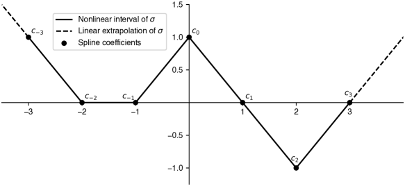
Figure 1: A LLS activation function with $T=1$ and $K=7$. The function is nonlinear in $[-3,3]$, and linearly extrapolated outside. At $x=1$, the second-order finite-difference is zero, which effectively removes one linear region. This behavior is favored by the regularization term $\frac{1}{T}\|\mathbf{Lc}\|_{1}$ which promotes sparse second-order finite differences and thereby decreases the number of effective linear regions.

Within LLS networks, the LLS can be initialized in many ways, some including popular activation functions such as ReLU, leaky ReLU, PReLU, or MaxMin. Further, the LLS activation functions can also be shared, which saves memory and training cost, and allows one to have one activation function per channel in convolutional neural networks.

3.3 Methods

To ensure that every activation function $\sigma$ is 1-Lipschitz, the absolute difference between any two consecutive coefficients must be at most $T$. Hence, the corresponding set of feasible coefficients is given by $\{\mathbf{c}\in\mathbb{R}^{K}:\|\mathbf{Dc}\|_{\infty}\leq T\}$. A first attempt at a minimization over this set has been made in Bohra et al. (2021). There, the authors use a method that divides each activation function by its maximum slope after each training step. In Section 3.3.1, we present an alternative projection scheme that is better suited to optimization and yields a much better performance in practice, while being just as fast. Additionally, we introduce a scaling parameter for each activation function, which facilitates the training and increases the performance of the network even further at a negligible computational cost.

3.3.1 Constrained Coefficients

The textbook approach to maintain the 1-Lipschitz property throughout an iterative minimization scheme would be to determine the least-squares projection onto $\{\mathbf{c}\in\mathbb{R}^{K}:\|\mathbf{Dc}\|_{\infty}\leq T\}$ at each iteration. This operation would preserve the mean of $\mathbf{c}$, as shown in Appendix C. Unfortunately, its computation is very expensive as it requires to solve a quadratic program after each training step and for each activation function. As substitute, we introduce a simpler projection SplineProj that also preserves the mean while being much faster to compute. In brief, SplineProj computes the finite-differences, clips them, sums them and adds a constant to the preservation of the mean.

Let us denote the Moore–Penrose pseudoinverse of $\mathbf{D}$ by $\mathbf{D}^{\dagger}$ and the vector of ones by $\mathbf{1}\in\mathbb{R}^{K}$. Further, we require the component-wise operation

$$\operatorname{Clip}_{T}(x)=\begin{cases}-T,&x<-T\\ x,&x\in[-T,T]\\ T,&x>T.\end{cases}$$ (12)

Proposition 3

The operation $\operatorname{SplineProj}$ defined as

$$\operatorname{SplineProj}(\mathbf{c})=\mathbf{D}^{\dagger}\operatorname{Clip}_{T}(\mathbf{Dc})+\mathbf{1}\frac{1}{K}\sum_{k=1}^{K}c_{k}$$ (13)

has the following properties:

1. it is a projection onto the set $\{\mathbf{c}\in\mathbb{R}^{K}:\|\mathbf{D}\mathbf{c}\|_{\infty}\leq T\}$;

2. it is almost-everywhere differentiable with respect to $\mathbf{c}$;

3. it preserves the mean of $\mathbf{c}$.

The proof of Proposition 3 can be found in Appendix C.

In gradient-based optimization, one usually handles domain constraints by projecting the variables back onto the feasible set after each gradient step. However, this turned out to be inefficient for neural networks in our experiments. Instead, we parameterize the LLS activation functions directly with $\operatorname{SplineProj}(\mathbf{c})$, which leads to unconstrained training. This strategy is in line with the popular spectral normalization of Miyato et al. (2018), where the weight matrices are unconstrained and parameterized using an approximate projection. For our parameterization approach, Property 2 of Proposition 3 is very important as it allows us to back-propagate through SplineProj during the optimization process. To compute SplineProj efficiently, we calculate $\mathbf{D}^{\dagger}$ in a matrix-free fashion with a cumulative sum. The computational cost of SplineProj is negligeable compared to the cost of constraining the linear layer to be 1-Lipschitz.

3.3.2 Scaling Parameter

We propose to increase the flexibility of our LLS activation functions by the introduction of an additional trainable scaling factor $\alpha$. Specifically, we propose the new activation function

$$\tilde{\sigma}(x)=\frac{1}{\alpha}\sigma(\alpha x).$$ (14)

With this scaling, $\tilde{\sigma}$ is nonlinear on $[k_{\text{min}}T/\alpha,k_{\text{max}}T/\alpha]$ and the Lipschitz constant

$$\operatorname{Lip}(\tilde{\sigma})=\sup_{x_{1},x_{2}\in\mathbb{R}}\frac{|\frac{1}{\alpha}\sigma(\alpha x_{1})-\frac{1}{\alpha}\sigma(\alpha x_{2})|}{|x_{1}-x_{2}|}=\sup_{x_{1},x_{2}\in\mathbb{R}}\frac{\frac{1}{\alpha}|\sigma(\alpha x_{1})-\sigma(\alpha x_{2})|}{\frac{1}{\alpha}|\alpha x_{1}-\alpha x_{2}|}=\operatorname{Lip}(\sigma)$$ (15)

is left unchanged. As detailed in Appendix D, the second-order total variation is preserved as well. Basically, $\alpha$ allows us to decrease the data-fitting term defined in (7) without breaking the constraints or increasing the complexity of the activation functions. Experimentally, we indeed found that the performance of LSS networks improves if we also optimize over $\alpha$. In contrast, the ReLU, AV, PReLU, GS, and HH activation functions are invariant to this parameter and do not benefit from it. In practice, the scaling parameter $\alpha$ is initialized as one and updated via standard stochastic gradient-based methods. Throughout our experiments, every LLS activation function has its own scaling parameter $\alpha$.

4 Experiments

With our experiments in Section 4.1, we gauge the expressivity of 1-Lip architectures that use either LLS or one of the activation functions from Section 2.2. Moreover, we assess the relevance of our proposed learning strategy for LLS. After this validation study, we benchmark our $1$-Lip architectures for the practical use-case of PnP image reconstruction in Section 4.2. There, we also prove important stability guarantees.

All 1-Lip networks are learned with the Adam optimizer (Kingma and Ba, 2015) and the default hyperparameters of its PyTorch implementation. For the parameters of the PReLU and HH activation functions, the learning rate is the same as for the weights of the network. The LLS networks use three different learning rates: $\eta$ for the weights, $\eta$/4 for the scaling parameters $\alpha$, and $\eta$/40 for the remaining parameters of the LLS. These ratios remain fixed throughout this section and, hence, only $\eta$ is going to be stated.

4.1 Evaluating the Expressivity

4.1.1 One-Dimensional Function Fitting

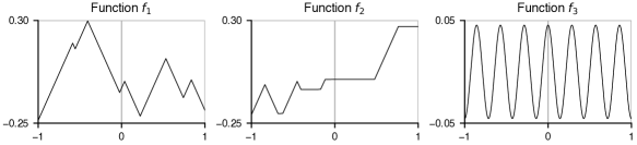
Figure 2: Three 1-Lipschitz functions that we attempt to fit with 1-Lip neural networks. All functions have zero mean over the interval $[-1,1]$.

Here, we use 1-Lip networks to fit the three 1-Lipschitz functions $f_{i}\colon[-1,1]\to\mathbb{R}$ in Figure 2. With this experiment, we aim to assess if the architectures achieve the full expressivity in the class of 1-Lipschitz functions on the real line. For $f_{1}$, we have $|\nabla f_{1}|=1$ almost everywhere. Hence, the GNP activation functions are expected to perform well and serve as a baseline against which we compare LLSs. The function $f_{2}$ alternates between $|\nabla f_{2}|=1$ and $|\nabla f_{2}|=0$. It was designed to test the ability of LLS networks to fit functions with constant regions. Lastly, we benchmark all methods on the highly varying function $f_{3}(x)=\sin(7\pi x)/7\pi$, which is challenging to fit under Lipschitz constraints. Additionally, we probe the impact of the two methods described in Sections 3.3.1 and 3.3.2 on the performance of the LLS networks by comparing the proposed implementation (denoted as LLS New) with the one from Bohra et al. (2021) (denoted as LLS Old), which relies on simple normalization.

Each network comes in two variants, namely with orthonormalization and spectral normalization of the weights. The mean squared error (MSE) loss is computed over 1000 uniformly sampled points from $[-1,1]$ for training, and a uniform partition of $[-1,1]$ with 10000 points for testing. For each instance, we tuned the width, the depth, and the hyperparameters of the network for the smallest test loss. ReLU networks have 10 layers and a width of 50; AV, PReLU, and HH networks have 8 layers and a width of 20; GS networks have 7 layers and a width of 20; LSS networks have 4 layers and a width of 10. We initialized the PReLU as the absolute value, we used GS with a group size of 5, and the LLS was initialized as ReLU and had a range of $[-0.5,0.5]$, 100 linear regions, and $\lambda=10^{-7}$ for the $\mathrm{TV}^{(2)}$ regularization. Every network relied on Kaiming initialization (He et al., 2015) and was trained 25 times with a batch size of 10 for 1000 epochs. The LLS networks always used $\eta=$2\text{\cdot}{10}^{-3}$$, while the other ones used $\eta=$4\text{\cdot}{10}^{-3}$$ for $f_{1}$, $f_{2}$ and $\eta=10^{-3}$ for $f_{3}$.

We report the median and the two quartiles of the test losses in Figure 3. For the spectral normalization, it appears that AV, PReLU, and HH tend to get stuck in local minima when fitting $f_{3}$ (the associated upper quartile of the loss is quite large). In return, we observe that LLS consistently outperforms the other architectures in all experiments. Particularly striking is the improvement of LLS New over LLS Old, which confirms the benefits of the two modules described in Sections 3.3.1 and 3.3.2. Accordingly, from now on, we drop LLS Old and only retain LLS New.

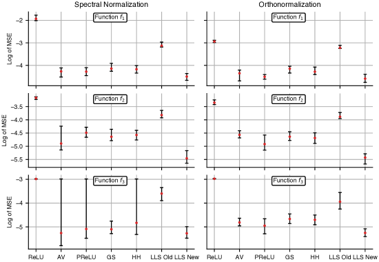
Figure 3: Fitting results for the functions from Figure 2. The red markers represent the median performance. The black bars represent the lower and upper quartiles, respectively.

4.1.2 High-Dimensional Function Fitting: Wasserstein Distances

The Wasserstein-1 distance $W_{1}$ is a metric for probability distributions. It has been used by Arjovsky et al. (2017) to improve the performance of GANs, which were first introduced in Goodfellow et al. (2014). Using the Kantorovich dual formulation (Villani, 2016), we can compute $W_{1}$ by solving an optimization problem over the space of 1-Lipschitz functions

$$W_{1}(P_{1},P_{2})=\sup_{\operatorname{Lip}(f)\leq 1}\mathbb{E}_{\mathbf{x}\sim P_{1}}[f(\mathbf{x})]-\mathbb{E}_{\mathbf{x}\sim P_{2}}[f(\mathbf{x})].$$ (16)

In (16), we can use a neural representations to parameterize the $f$ for optimization purposes. Since expressive architectures are very important in this context, we get another good benchmark. Experimentally, Anil et al. (2019) observed that orthonormalization of the linear layers is superior to spectral normalization for this task. Hence, we only use the former in our experiments. Further, Gulrajani et al. (2017) have shown that, under reasonable assumptions, any $f^{*}$ that maximizes (16) satisfies $|\nabla f^{*}|=1$ almost everywhere. Hence, GNP architectures are expected to perform better. In general, estimating $W_{1}$ for high-dimensional distributions is very challenging, see Korotin et al. (2022) for a recent survey.

Gaussian Mixtures

In our first setting, the distributions are

$$P_{1}=X_{1}Z_{1}+(1-X_{1})Z_{2}\quad\text{ and }\quad P_{2}=X_{2}Z_{3}+(1-X_{2})Z_{4},$$ (17)

where $\mathbb{P}(X_{k}=0)=\mathbb{P}(X_{k}=1)=1/2$ for $k=1,2$ and $Z_{k}\sim\mathcal{N}(\mathbf{\mu}_{k},\mathbf{\Sigma}_{k})$ for $k=1,...,4$. The $\mathbf{\mu}_{k}\in\operatorname{{\mathbb{R}}}^{N}$ and $\mathbf{\Sigma}_{k}\in\operatorname{{\mathbb{R}}}^{N,N}$, $N\in\{5,10,20\}$, are random with $(\mathbf{\mu}_{k})_{n}\sim\mathcal{N}(0,1)$ and $\mathbf{\Sigma}_{k}=\mathbf{A}_{k}^{T}\mathbf{A}_{k}$ with $(\mathbf{A}_{k})_{nm}\sim\mathcal{N}(0,1)$ and $1\leq n,m\leq N$. For each instance, we tuned the width and the depth of the fully connected neural representation for best performance. Irrespective of $N$, ReLU architectures had 30 layers and a width of 1024; all other architectures had 10 layers and a width of 2048. The PReLUs were initialized as the ReLU for $N\in\{5,10\}$, and as MaxMin for $N=20$. We used GS with a group size of 2 for $N\in\{5,20\}$ and 4 for $N=4$. The LLS had 50 linear regions for $N=5$ and 100 for $N\in\{10,20\}$. Their range was $[-1,1]$, $[-5,5]$, and $[-10,10]$ for $N=$ 5, 10 and 20, respectively. Further, we set $\lambda=10^{-10}$ for the $\mathrm{TV}^{(2)}$ regularization, and initialized the LLS as the ReLU for $N\in\{5,10\}$ and as MaxMin for $N=20$. The additional LLS coefficients increased the architecture parameters by at most 0.7$\%$. All neural representations used orthogonal initialization (Saxe et al., 2014) and were optimized for 10000 gradient steps with $\eta=$5\text{\cdot}{10}^{-3}$$ and batches of 4096 samples.

In Table 1, we report the mean and standard deviation over five runs of the Monte Carlo estimation for $W_{1}$ as in (16) with the learned $f$ and $10^{5}$ samples. ReLU leads to an estimate that is significantly lower than the others, which is, most likely, due to its lack of expressivity. Otherwise, the estimates are quite similar. LLS has the best estimate for $N\in\{5,10\}$ but is slightly outperformed for $N=20$.

Table 1: Estimated Wasserstein distance for the Gaussian mixtures.

$N$	ReLU	AV	PReLU	GS	HH	LLS
5	2.009/0.004	2.271/0.006	2.279/0.006	2.271/0.006	2.272/0.006	2.283/0.006
10	5.960/0.014	6.461/0.011	6.465/0.012	6.475/0.012	6.461/0.012	6.486/0.011
20	11.638/0.007	13.187/0.012	13.245/0.012	13.251/0.012	13.247/0.012	13.243/0.012

MNIST

Here, $P_{1}$ is a uniform distribution over a set of real MNIST images and $P_{2}$ is the generator distribution of a GAN trained to generate MNIST images. The architecture of this GAN is taken from Chen et al. (2016). All neural representations of $f$ are fully connected with a width of 1024, and various depths. They were optimized 5 times each for 2000 epochs with $\eta=$2\text{\cdot}{10}^{-3}$$ and orthogonal initialization (Saxe et al., 2014). For a depth of 3, GS has group size of 8, and PReLU and LLS were initialized as the absolute value. For a depth of 5 or 7, GS has a group size of 2, and PReLU and LLS were initialized as MaxMin. The LLS have a range of $[-0.15,0.15]$, 20 linear regions, and $\lambda=10^{-10}$. Their coefficients only increase the total number of parameters in the architecture by 2%. We optimize the neural representation on 54000 images from the MNIST training set and use the 6000 remaining ones as validation set. The test set contains 10000 MNIST images.

In Table 2, we report the estimated $W_{1}$ metric between the MNIST images of the test set and the ones generated by the GAN. Again, ReLU leads to an estimate that is significantly lower than the others. Otherwise, the results are more or less similar except for AV and HH with depth 7 and 3, respectively, which are worse than the others.

Table 2: Mean and standard deviation of the estimated Wasserstein distance over five trials for several architectures.

Depth	ReLU	AV	PReLU	GS	HH	LLS
3	0.727/0.001	1.190/0.002	1.190/0.002	$1.189/0.001$	1.165/0.001	1.190/0.002
5	$0.881/0.001$	$1.368/0.003$	$1.371/0.002$	$1.369/0.002$	$1.369/0.002$	1.373/0.003
7	0.960/0.001	$1.406/0.008$	$1.437/0.002$	$1.436/0.001$	1.440/0.003	$1.439/0.001$

4.1.3 1-Lipschitz Wasserstein GAN Training

We train Wasserstein GANs to generate MNIST images. To this end, we use the same framework and optimization process as Anil et al. (2019), where the discriminators have strict Lipschitz constraints instead of the commonly used relaxation in terms of a gradient penalty. On the contrary, the generators themselves are unconstrained. Thus, we use ReLUs as their activation functions and only plug the activation functions from Section 2.2 into the discriminator. Here, GS has a group size of 2, PReLU was initialized as MaxMin, LLS was initialized as the absolute value, has range $[-0.1,0.1]$, 20 linear regions, and $\lambda=10^{-6}.$ The spline coefficients only increase the total number of parameters in the neural network by 0.2%. The Wasserstein GANs were trained on the MNIST training set.

We report the inception score on the MNIST test set using the implementation from Li et al. (2017) in Table 3. As expected, the limited expressivity of the ReLU leads to the lowest score. LLS yields the best score of all schemes and its ability to generate realistic digits can be appreciated visually in Figure 4. Still, we should keep in mind that the main purpose of this experiment is an expressivity comparison and not generative performance.

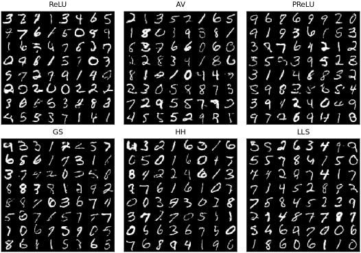
Figure 4: Digits generated by the Wasserstein GANs with different activation functions.

Table 3: Inception scores for MNIST digit generation.

	ReLU	AV	PReLU	GS	HH	LLS
Inception score	1.88	2.19	2.13	2.17	2.07	2.38

4.2 Image Reconstruction via Plug-and-Play

Many image-reconstruction tasks can be formulated as a linear inverse problem. Specifically, the task is to recover an image $\mathbf{x}\in\mathbb{R}^{n}$ from the noisy measurement

$$\mathbf{y}=\mathbf{Hx}+\mathbf{n}\in\mathbb{R}^{m},$$ (18)

where $\mathbf{H}\in\mathbb{R}^{m\times n}$ is a measurement operator and $\mathbf{n}\in\mathbb{R}^{m}$ is random noise. Problem (18) is nondeterministic and often ill-posed, in the sense that multiple images yield the same measurements. To make (18) well-posed, one usually incorporates prior knowledge about the unknown image $\mathbf{x}$ by adding regularization. This leads to the reconstruction problem

$$\min_{\mathbf{x}\in\mathbb{R}^{n}}f(\mathbf{y},\mathbf{H}\mathbf{x})+g(\mathbf{x}),$$ (19)

where $f\colon\operatorname{{\mathbb{R}}}^{m}\times\operatorname{{\mathbb{R}}}^{m}\to\operatorname{{\mathbb{R}}}^{+}$ is a data-fidelity term and $g\colon\operatorname{{\mathbb{R}}}^{n}\to\operatorname{{\mathbb{R}}}^{+}$ is a prior that favors certain types of solutions. If $f$ is differentiable and $g$ is convex, (19) can be minimized by the iterative forward-backward splitting (FBS) algorithm (Combettes and Wajs, 2005) with

$$\mathbf{x}^{k+1}=\operatorname{prox}_{\alpha g}\bigl{(}\mathbf{x}^{k}-\alpha\boldsymbol{\nabla}f(\mathbf{y},\mathbf{Hx}^{k})\bigr{)}.$$ (20)

Here, the proximal operator of $g$ is defined as $\operatorname{prox}_{g}(\mathbf{z})=\operatorname*{arg\,min}_{\mathbf{x}\in\operatorname{{\mathbb{R}}}^{d}}\tfrac{1}{2}\|\mathbf{x}-\mathbf{z}\|^{2}+g(\mathbf{x})$. The idea behind PnP algorithms (Venkatakrishnan et al., 2013) is to replace $\operatorname{prox}_{\alpha g}$ with a generic denoiser $D\colon\mathbb{R}^{n}\to\mathbb{R}^{n}$. While not necessarily corresponding to an explicit regularizer $g$, this approach has led to improved results compared to conventional methods as it allows the use of powerful deep-learning-based denoisers, as done in Ryu et al. (2019); Sun et al. (2021); Ye et al. (2018). The convergence of the PnP-FBS iterations

$$\mathbf{x}^{k+1}=D\bigl{(}\mathbf{x}^{k}-\alpha\boldsymbol{\nabla}f(\mathbf{y},\mathbf{Hx}^{k})\bigr{)}$$ (21)

can be guaranteed (Hertrich et al., 2021, Proposition 15) if

• $D$ is averaged, i.e., of the form $D=\beta R+(1-\beta)\operatorname{Id}$ with a 1-Lipschitz $R$ and $\beta\in(0,1)$;

• $f(\mathbf{y},\mathbf{H}\cdot)$ is convex, differentiable with $L$-Lipschitz gradient, and $\alpha\in(0,2/L)$.

In addition, we now prove the Lipschitz continuity of the data-to-reconstruction map, which is an important property for image reconstruction methods.

Proposition 4

Let $\mathbf{x}_{1}^{*}$ and $\mathbf{x}_{2}^{*}$ be fixed points of (21) for measurements $\mathbf{y}_{1}$ and $\mathbf{y}_{2}$, respectively. If $D$ is averaged with $\beta\leq 1/2$ and $f(\mathbf{y},\mathbf{Hx})=\frac{1}{2}\|\mathbf{y}-\mathbf{Hx}\|_{2}^{2}$, then it holds that

$$\|\mathbf{H}\mathbf{x}_{1}^{*}-\mathbf{H}\mathbf{x}_{2}^{*}\|\leq\|\mathbf{y}_{1}-\mathbf{y}_{2}\|.$$ (22)

If $\mathbf{H}$ is invertible, this yields the direct relation

$$\|\mathbf{x}_{1}^{*}-\mathbf{x}_{2}^{*}\|\leq\frac{1}{\sigma_{\text{min}}(\mathbf{H}^{T}\mathbf{H})}\|\mathbf{y}_{1}-\mathbf{y}_{2}\|.$$ (23)

Under slightly stronger constraints on $D$, we also have a result for non-invertible $\mathbf{H}$.

Proposition 5

In the setting of Proposition 4, it holds for $K$-Lipschitz $D$, $K<1$, that

$$\|\mathbf{x}_{1}^{*}-\mathbf{x}_{2}^{*}\|\leq\frac{\alpha\|\mathbf{H}\|K}{1-K}\|\mathbf{y}_{1}-\mathbf{y}_{2}\|.$$ (24)

Propositions 4 and 5 are proven in Appendix E. In principle, the model (19) leads to better data consistency than the one provided by the end-to-end neural network frameworks that directly reconstruct $\mathbf{x}$ from $\mathbf{y}$. Those latter approaches are also known to suffer from stability issues (Antun et al., 2020) and, more importantly, have been found to remove or hallucinate structure (Nataraj and Otazo, 2020; Muckley et al., 2021), which is unacceptable in diagnostic imaging. In sharp contrast, our PnP approach (21) comes with the stability estimates (22), (23) and (24) which typically do not hold for other PnP methods.

4.2.1 Learning a Denoiser for PnP

A good denoising network is the backbone of most PnP methods. Unfortunately, most common architectures (Ronneberger et al., 2015; Zhang et al., 2017; Liang et al., 2021) are not natively 1-Lipschitz. They rely on dedicated modules designed to improve the denoising performance, such as skip connections, batch normalization, and attention modules. These make it challenging to build provably averaged denoisers. Instead, we use a plain CNN architecture that is equivalent to the DnCNN of Zhang et al. (2017) without the residual. This architecture is easy to constrain and still provides competitive performance. In detail, we train 1-Lip denoisers that are composed of 8 orthogonal convolutional layers and the activation functions from Section 2.2. The convolutional layers are parameterized with the BCOP framework (Li et al., 2019) and have kernels of size $(3\times 3)$. For the LLS, we take 64 channels. To compensate for the additional spline parameters, we train every other model with 68 channels.

The training dataset consists of 238400 patches of size $(40\times 40)$ taken from the BSD500 image dataset (Arbeláez et al., 2011). All images take values in $[0,1]$. We train denoisers for Gaussian noise with standard deviation $\sigma=5/255,10/255,15/255$. All denoisers are trained for 50 epochs with a batch size of 128, $\eta=$4\text{\cdot}{10}^{-5}$$, and the MSE loss function. The PReLU activation functions were initialized as the absolute value. GS has a group size of 2. The LLS activation functions have 50 linear regions, a range of 0.1, and were initialized as the identity. In this experiment, we also investigated the effect of the $\mathrm{TV}^{(2)}$ regularization parameter $\lambda$ on the performance and the number of linear regions in the LLSs. The performances on the BSD68 test set are provided in Table 5. For each noise level, LLS performs best, and, as expected, ReLU is doing worse than all the others.

The number of linear regions for the LLS $\sigma_{\ell,n}$ is equal to $\frac{1}{T}\|\mathbf{Lc}_{\ell,n}\|_{0}+1$. This metric can overestimate the number of linear regions due to numerical imprecisions. Instead, we define the effective number of linear regions as $(|\{1\leq k\leq K_{\ell,n}:|(\mathbf{L}\mathbf{c}_{\ell,n})_{k}|>0.01\}|+1)$. For each LSS network, we report in Table 5 the average number of effective linear regions (AELR) over all the $\sigma_{\ell,n}$. An AELR close to one indicates that the majority of neurons become skip connection, which corresponds to a simplification of the network. Without regularization, the $\sigma_{\ell,n}$ have an AELR of 8.07 to 9.24 out of the 50 available linear regions. The $\mathrm{TV}^{(2)}$ regularization drastically sparsifies the $\sigma_{\ell,n}$. With $\lambda\in[10^{-6},10^{-4}]$, the AELR is between 1.07 and 1.44, which is a large decrease without degradation in the denoising performances. For $\lambda=10^{-3}$, the $\sigma_{\ell,n}$ are even further sparsified at the cost of a small loss of performance. We observe a significant loss of performance when $\lambda$ is increased to $10^{-2}$, where the network is almost an affine mapping. Notice that the AELR is 2 for ReLU and AV, meaning that LLS outperforms them while being simpler. Another interesting observation is that, despite being very sparse on average, the LLS networks with $\lambda\in[10^{-6},10^{-3}]$ have at least one $\sigma_{\ell,n}$ with at least three linear regions. This suggests that most of the common activation functions might be suboptimal as they have only two linear regions.

Table 4: PSNR and SSIM values on BSD68 for each activation function and noise level.

Noise level	$\sigma=5/255$		$\sigma=10/255$		$\sigma=15/255$
Metric	PSNR	SSIM	PSNR	SSIM	PSNR	SSIM
ReLU	36.10	0.9386	31.92	0.8735	29.76	0.8203
AV	36.58	0.9499	32.33	0.8889	30.09	0.8375
PReLU	36.58	0.9498	32.25	0.8887	30.11	0.8367
GS	36.54	0.9489	32.23	0.8845	30.11	0.8346
HH	36.47	0.9476	32.25	0.8866	30.11	0.8350
LLS ($\lambda=0$)	36.85	0.9540	32.59	0.8978	30.35	0.8464
LLS ($\lambda=10^{-6}$)	36.86	0.9546	32.55	0.8962	30.38	0.8479
LLS ($\lambda=10^{-5}$)	36.86	0.9543	32.55	0.8960	30.34	0.8455
LLS ($\lambda=10^{-4}$)	36.82	0.9534	32.57	0.8970	30.36	0.8468
LLS ($\lambda=10^{-3}$)	36.63	0.9497	32.47	0.8924	30.31	0.8437
LLS ($\lambda=10^{-2}$)	35.15	0.9142	32.00	0.8782	29.73	0.8156

Table 5: Average number of effective linear regions (AELR) for several $\lambda$ and noise levels.

Noise level	$\lambda=0$	$\lambda=10^{-6}$	$\lambda=10^{-5}$	$\lambda=10^{-4}$	$\lambda=10^{-3}$	$\lambda=10^{-2}$
$\sigma=5/255$	9.24	1.21	1.11	1.07	1.02	1.00
$\sigma=10/255$	8.76	1.24	1.15	1.14	1.06	1.01
$\sigma=15/255$	8.07	1.44	1.24	1.25	1.10	1.02

4.2.2 Numerical Results for PnP-FBS

Now, we want to deploy the learned denoisers $D_{\sigma}$ (which are learned with $\lambda=10^{-6}$ for LLS) in the PnP-FBS algorithm for image reconstruction, where we use the data-fidelity term $f(\mathbf{y},\mathbf{Hx})=\frac{1}{2}\|\mathbf{y}-\mathbf{Hx}\|_{2}^{2}$. To ensure convergence, we set $\alpha=1/\|\mathbf{H}^{*}\mathbf{H}\|$, and we tune the noise level $\sigma$ of $D_{\sigma}$ on the validation set over $\sigma=5/255,10/255,15/255$. To further adapt the denoising strength and to make them $\beta$-averaged, we replace the $D_{\sigma}$ by $D_{\sigma,\beta}=\beta D_{\sigma}+(1-\beta)\operatorname{Id}$, where the parameter $\beta\in[0,1)$ is also tuned on the validation set. In our experiments, we actually noticed that the best $\beta$ is always lower than 1/2, which means that the conditions in Proposition 4 are met. As the GS activation function involves sorting of the feature map along its 68 channels, it takes significantly more time than the other activation functions. Hence, it is impractical to tune the hyperparameters, and we do not use it for this image reconstruction experiment.

Single-Coil MRI

Here, we want to recover $\mathbf{x}$ from $\mathbf{y}=\mathbf{MFx}+\mathbf{n}\in\mathbb{C}^{M}$, where $\mathbf{M}$ is a subsampling mask (identity matrix with some missing entries), $\mathbf{F}$ is the discrete Fourier transform matrix, and $\mathbf{n}$ is a realization of a complex-valued Gaussian noise characterized by $\sigma_{\mathbf{n}}$ for the real and imaginary parts. This noise level is not to be confused with the noise level $\sigma$ that appears in $D_{\sigma,\beta}$. We use fully sampled knee MR images of size $(320\times 320)$ from the fastMRI dataset (Knoll et al., 2020) as ground truths. Specifically, we create validation and test sets consisting of 100 and 99 images, respectively, which are individually normalized within the range $[0,1]$. For our experiments, the subsampling mask $\mathbf{M}$ is specified by two parameters: the acceleration $M_{\text{acc}}$ and the center fraction $M_{\text{cf}}$. It selects the $\lfloor 320M_{\text{cf}}\rfloor$ columns in the center of the k-space (low frequencies). Further, it selects columns uniformly at random from the other regions in the k-space such that the total number of selected columns is $\lfloor 320/M_{\text{acc}}\rfloor$. The measurements are simulated with $\sigma_{\mathbf{n}}=0.01$.

The reconstruction performances over the test set are reported in Table 8. We observe a significant gap between LLS and the other activation functions for both masks $M$ in terms of PSNR and SSIM. Actually, LLS outperforms the other schemes on every single image from the test set. In Figure 7, we observe stripe-like structures in the zero-fill reconstruction. These are typical aliasing artifacts that result from the subsampling in the horizontal direction in Fourier space. They are significantly reduced in the LLS reconstruction.

Multi-Coil MRI with 15 Coils

Here, the data is given by $\mathbf{y}=(\mathbf{y}_{1},\ldots,\mathbf{y}_{15})$ with $\mathbf{y}_{k}=\mathbf{MFS}_{k}\mathbf{x}+\mathbf{n}_{k}$ and complex-valued diagonal matrices $\mathbf{S}_{k}\in\mathbb{C}^{n\times n}$ (called sensitivity maps). These maps were estimated from the data $\mathbf{y}$ using the ESPIRiT algorithm (Uecker et al., 2014), which is part of the BART toolbox (Uecker et al., 2013). Again, the ground-truth images are from the fastMRI dataset (Knoll et al., 2020), but both with (PDFS) and without (PD) fat suppression. The Fourier subsampling is performed with the parametric Cartesian mask from before. Gaussian noise with standard deviation $\sigma_{\mathbf{n}}=$2\text{\cdot}{10}^{-3}$$ is added to the real and imaginary parts of the measurements. The reconstruction performances over the test set are reported in Table 8. Again, we observe a significant gap in terms of PSNR and SSIM between LLS and the other activation functions for both masks. LLS outperforms the other schemes on every single image from the test set.

Computed Tomography (CT)

The groundtruth comes from human abdominal CT scans for 10 patients provided by Mayo Clinic for the low-dose CT Grand Challenge (McCollough, 2016). The validation set consists of 6 images taken uniformly from the first patient of the training set from Mukherjee et al. (2021). We use the same test set as Mukherjee et al. (2021), more precisely, 128 slices with size $(512\times 512)$ that correspond to one patient. The data $\mathbf{y}$ is simulated through a parallel-beam acquisition geometry with 200 angles and 400 detectors. These measurements are corrupted by Gaussian noise with standard deviation $\sigma_{\mathbf{n}}\in\{0.5,1,2\}$. The reconstruction performance in terms of PSNR and SSIM over the test set are reported in Table 8. Again, we observe a significant gap between LLS and the other activation functions. LLS outperforms the other schemes on every single image from the testing set. Reconstructions for one image are reported in Figure 7.

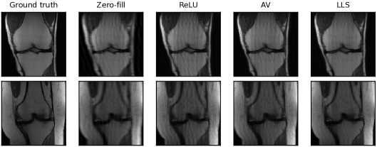
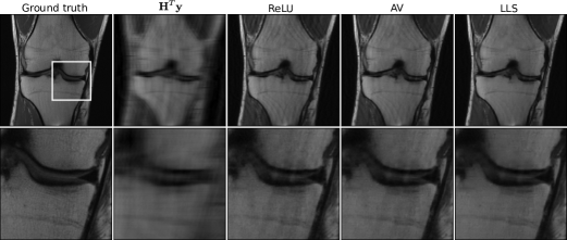
Figure 5: The ground truth, the zero-fill reconstruction $\mathbf{H}^{T}\mathbf{y}$, and the PnP-FBS reconstruction using networks with ReLU, LLS, and AV for the single-coil MRI experiment.

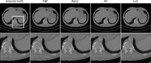
Figure 6: The ground truth, the zero-fill reconstruction $\mathbf{H}^{T}\mathbf{y}$, and the PnP-FBS reconstruction using networks with ReLU, LLS, and AV for the multi-coil MRI experiment.

Figure 7: Reconstructions for the CT experiment. We report the ground truth, the filtered backprojection and the PnP-FBS reconstruction using networks with ReLU, LLS, and AV.

Table 6: PSNR and SSIM values for the single-coil MRI reconstruction experiment.

($M_{\text{acc}}$, $M_{\text{cf}}$)	(4, 0.08)		(6, 0.06)
Metric	PSNR	SSIM	PSNR	SSIM
Zero-fill	27.55	0.6895	25.55	0.6223
ReLU	29.97	0.7574	26.87	0.6781
AV	30.61	0.7721	27.35	0.6921
PReLU	30.58	0.7716	27.32	0.6906
HH	30.55	0.7696	27.34	0.6887
LLS	31.54	0.7924	28.04	0.7108

Table 7: PSNR and SSIM values for the multi-coil MRI experiment.

($M_{\text{acc}}$, $M_{\text{cf}}$)		(4, 0.08)				(8, 0.04)
	PSNR		SSIM		PSNR		SSIM
	PD	PDFS	PD	PDFS	PD	PDFS	PD	PDFS
Zero-fill	27.71	29.94	0.751	0.759	23.80	27.19	0.648	0.681
ReLU	37.21	37.06	0.929	0.915	31.37	32.57	0.837	0.822
AV	37.81	37.48	0.935	0.919	31.82	32.95	0.845	0.829
PReLU	37.71	37.51	0.934	0.919	31.67	33.11	0.845	0.832
HH	37.66	37.39	0.933	0.919	31.68	32.91	0.843	0.829
LLS	38.68	37.96	0.943	0.924	32.75	33.61	0.859	0.835

Table 8: PSNR and SSIM values for the CT experiment.

	$\sigma_{\mathbf{n}}$=0.5		$\sigma_{\mathbf{n}}$=1		$\sigma_{\mathbf{n}}$=2
	PSNR	SSIM	PSNR	SSIM	PSNR	SSIM
FBP	32.14	0.697	27.05	0.432	21.29	0.204
ReLU	36.94	0.914	33.65	0.860	30.34	0.782
AV	37.15	0.926	34.19	0.885	31.07	0.813
PReLU	37.18	0.927	34.21	0.887	30.87	0.812
HH	36.94	0.918	34.11	0.877	30.92	0.809
LLS	38.19	0.931	35.15	0.897	31.85	0.844

5 Conclusion

In this paper, we proposed a framework to efficiently train $1$-Lipschitz neural networks with learnable linear-spline activation functions. First, we formulated the training stage as an optimization task and showed that the solution set contains networks with linear-spline activation functions. Our implementation of this framework embeds the required $1$-Lipschitz constraint on the splines directly into the forward pass. Further, we added learnable scaling factors, which preserve the Lipschitz constant of the splines and enhance the overall expressivity of the network. For the practically relevant PnP image reconstruction, our approach significantly outperforms $1$-Lipschitz architectures that rely on other (popular) activation functions such as the parametric ReLU and Householder. In this setting, classical choices such as ReLU suffer from limited expressivity and should not be used. Our observations are a starting point for the exploration of other architectural constraints and learnable non-component-wise activation functions within the framework of $1$-Lipschitz networks.

Appendix A Proof of Proposition 1

We express the activation functions in terms of each other using weights $\mathbf{W}_{k}$ with $\|\mathbf{W}_{k}\|_{2}\leq 1$. Choose $B$ such that $x+B>0$ for all $x\in D$ and any pre-activation in the network.

AV as Expressive as PReLU:

We can express AV using PReLU with $a=-1$. For the other direction, we have that

$$\operatorname{PReLU}_{a}(x)$$

$$= \begin{bmatrix}\sqrt{(1+a)/2}&-\sqrt{(1-a)/2}\end{bmatrix}\operatorname{AV}\left(\begin{bmatrix}\sqrt{(1+a)/2}\\ \sqrt{(1-a)/2}\end{bmatrix}x+\begin{bmatrix}\sqrt{(1+a)/2}B\\ 0\end{bmatrix}\right)-\frac{1+a}{2B}.$$ (25)

AV as Expressive as GS:

This was already proven in Anil et al. (2019), but we include the expressions for the sake of completeness. It holds that

$$\begin{bmatrix}\max(x_{1})\\ \min(x_{2})\end{bmatrix}=\mathbf{M}\operatorname{AV}\left(\mathbf{M}\begin{bmatrix}x_{1}\\ x_{2}\end{bmatrix}+\begin{bmatrix}B\\ 0\end{bmatrix}\right)-\begin{bmatrix}\sqrt{2}B\\ 0\end{bmatrix},$$ (26)

where

$$\mathbf{M}=\frac{1}{\sqrt{2}}\begin{bmatrix}1&1\\ 1&-1\end{bmatrix}.$$ (27)

For the reverse direction, we have that

$$\operatorname{AV}(x)=\begin{bmatrix}\frac{1}{\sqrt{2}}&-\frac{1}{\sqrt{2}}\end{bmatrix}\operatorname{MaxMin}\left(\begin{bmatrix}\frac{1}{\sqrt{2}}\\ \frac{1}{\sqrt{2}}\end{bmatrix}x\right).$$ (28)

GS as Expressive as HH:

For $\mathbf{v}=\frac{1}{\sqrt{2}}(1,-1)$ we have that $\text{HH}_{\mathbf{v}}=\text{MaxMin}$. Further, we can also express $\text{HH}_{\mathbf{v}}$ using MaxMin as

$$\operatorname{HH}_{\mathbf{v}}\left(\mathbf{z}\right)=\mathbf{R}(\mathbf{v})\operatorname{MaxMin}\bigl{(}\mathbf{R}(\mathbf{v})^{T}\mathbf{z}\bigr{)},$$ (29)

where $\mathbf{R}(\mathbf{v})$ is the rotation matrix

$$\mathbf{R}(\mathbf{v})=\begin{bmatrix}\cos\gamma(v_{1},v_{2})&-\sin\gamma(v_{1},v_{2})\\ \sin\gamma(v_{1},v_{2})&\cos\gamma(v_{1},v_{2})\end{bmatrix}\text{ with }\gamma(v_{1},v_{2})=\frac{\pi}{4}+2\arctan\frac{v_{2}}{1+v_{1}}.$$ (30)

$\blacksquare$

Appendix B Proof of Theorem 2

Without loss of generality, we assume that all biases in $f_{\theta}$ are zero as they can be integrated into the $\sigma_{\ell}$. First, we show that solutions for (7) exist. For $\ell=1,\ldots,(L-1)$ and $\bar{\sigma}_{1}=\sigma_{1}$, we can iteratively replace the $\sigma_{\ell}$ in $f_{\theta}$ by $u_{\ell}$ without changing the output as in

$$\sigma_{\ell+1}\bigl{(}\mathbf{W}_{\ell+1}\bar{\sigma}_{\ell}(\mathbf{z})\bigr{)}=\sigma_{\ell+1}\bigl{(}\mathbf{W}_{\ell+1}(\bar{\sigma}_{\ell}(\mathbf{z})-\bar{\sigma}_{\ell}(\mathbf{0}))+\mathbf{W}_{\ell+1}\bar{\sigma}_{\ell}(\mathbf{0})\bigr{)}=\bar{\sigma}_{\ell+1}\bigl{(}\mathbf{W}_{\ell}u_{\ell}(\mathbf{z})\bigr{)},$$ (31)

where $u_{\ell}=\bar{\sigma}_{\ell}-\bar{\sigma}_{\ell}(\mathbf{0})\in\operatorname{BV}^{(2)}(\operatorname{{\mathbb{R}}})$ and $\bar{\sigma}_{\ell+1}=\sigma_{\ell+1}(\,\cdot+\mathbf{W}_{\ell}\bar{\sigma}_{\ell}(\mathbf{0}))$. For the last layer, we set

$$\bar{\sigma}_{L}\bigl{(}\mathbf{W}_{L}u_{L-1}(\mathbf{z})\bigr{)}=u_{L}\bigl{(}\mathbf{W}_{L}u_{L-1}(\mathbf{z})\bigr{)}+\mathbf{a}_{L},$$ (32)

where $u_{L}=\bar{\sigma}_{L}-\bar{\sigma}_{L}(\mathbf{0})\in\operatorname{BV}^{(2)}(\operatorname{{\mathbb{R}}})$ and $\mathbf{a}_{L}=\bar{\sigma}_{L}(\mathbf{0})=f_{\theta}(\mathbf{0})\in\operatorname{{\mathbb{R}}}^{N_{L}}$. Consequently, $\mathrm{TV}^{(2)}\left(u_{\ell,n}\right)=\mathrm{TV}^{(2)}\left(\sigma_{\ell,n}\right)$ and $u_{\ell}(\mathbf{0})=\mathbf{0}$. Hence, a solution of (7) exists if the restricted problem

$$\operatorname*{arg\,min}_{\begin{subarray}{c}\mathbf{W}_{\ell},\sigma_{\ell,n}\in\operatorname{BV}^{(2)}(\mathbb{R})\\ \text{s.t.}\operatorname{Lip}(\sigma_{\ell,n})\leq 1,\,\|\mathbf{W}_{\ell}\|\leq 1\\ \sigma_{\ell,n}(0)=0,|\sigma_{\ell,n}(1)|\leq 1\\ \mathbf{a}_{L}\in{\mathbb{R}}^{N_{L}}\end{subarray}}\left(\sum_{m=1}^{M}E\bigl{(}\mathbf{y}_{m},f_{\theta}\left(\mathbf{x}_{m}\right)+\mathbf{a}_{L}\bigr{)}+\lambda\sum_{\ell=1}^{L}\sum_{n=1}^{N_{\ell}}\mathrm{TV}^{(2)}\left(\sigma_{\ell,n}\right)\right)$$ (33)

has a nonempty solution set. Since $f_{\theta}$ is $1$-Lipschitz, it holds that

$$\|f_{\theta}(\mathbf{x}_{m})-\mathbf{a}_{L}\|=\|f_{\theta}(\mathbf{x}_{m})-f_{\theta}(\mathbf{0})\|\leq\|\mathbf{x}_{m}\|.$$ (34)

In addition, we have that

$$2\|\mathbf{a}_{L}\|=\|(f_{\theta}(\mathbf{x}_{m})-\mathbf{a}_{L})-(f_{\theta}(\mathbf{x}_{m})+\mathbf{a}_{L})\|\leq\|f_{\theta}(\mathbf{x}_{m})-\mathbf{a}_{L}\|+\|f_{\theta}(\mathbf{x}_{m})+\mathbf{a}_{L}\|$$ (35)

and, therefore, that

$$\|f_{\theta}(\mathbf{x}_{m})+\mathbf{a}_{L}\|\geq 2\|\mathbf{a}_{L}\|-\|\mathbf{x}_{m}\|.$$ (36)

The fact that $E$ is coercive and positive implies that

$$\lim_{\|\mathbf{a}_{L}\|\to+\infty}\sum_{m=1}^{M}E\bigl{(}\mathbf{y}_{m},f_{\theta}\left(\mathbf{x}_{m}\right)+\mathbf{a}_{L}\bigr{)}=+\infty.$$ (37)

We conclude that there exists a constant $A>0$ such that it suffices to minimize over $\|\mathbf{a}_{L}\|\leq A$ in (33). Now, the remaining steps for the proof of existence are the same as in the proof of Theorem 3 in Aziznejad et al. (2020).

For the second part of the claim, we follow the reasoning in Unser (2019). Let $f_{\tilde{\theta}}$ be a solution of (7) with weights $\tilde{\mathbf{W}}_{\ell}$, biases $\tilde{\mathbf{b}}_{\ell}$, and activation functions $\tilde{\sigma}_{\ell,n}$. When evaluating $f_{\tilde{\theta}}$ at the data point $\mathbf{x}_{m}$, we iteratively generate vectors $\mathbf{z}_{m,\ell},\tilde{\mathbf{y}}_{m,\ell}\in\mathbb{R}^{N_{\ell}}$ as follows.

1. Initialization (input of the network): $\tilde{\mathbf{y}}_{m,0}=\mathbf{x}_{m}$.

2. Iterative update: For $\ell=1,\ldots,L$, calculate

   $$\mathbf{z}_{m,\ell}=\left(z_{m,\ell,1},\ldots,z_{m,\ell,N_{\ell}}\right)=\tilde{\mathbf{W}}_{\ell}\tilde{\mathbf{y}}_{m,\ell-1}+\tilde{\mathbf{b}}_{\ell}$$ (38)

   and define $\tilde{\mathbf{y}}_{m,\ell}=\left(\tilde{y}_{m,\ell,1},\ldots,\tilde{y}_{m,\ell,N_{\ell}}\right)\in\mathbb{R}^{N_{\ell}}$ as

   $$\tilde{y}_{m,\ell,n}=\tilde{\sigma}_{\ell,n}\left(z_{m,\ell,n}\right),\quad n=1,\ldots,N_{\ell}.$$ (39)

We directly observe that $\tilde{\mathbf{y}}_{m,\ell}$ only depends on the values of $\tilde{\sigma}_{\ell,n}\colon\mathbb{R}\rightarrow\mathbb{R}$ at the locations $z_{m,\ell,n}$. Hence, the optimal $\tilde{\sigma}_{\ell,n}$ are the $1$-Lipschitz interpolations between these points with minimal second-order total variation, as the regularizers for $\tilde{\sigma}_{\ell,n}$ in (33) do not depend on each other. More precisely, the $\tilde{\sigma}_{\ell,n}$ solve the problem

$$\tilde{\sigma}_{\ell,n}\in\operatorname*{arg\,min}_{\begin{subarray}{c}f\in\mathrm{BV}^{(2)}(\mathbb{R})\\ \text{s.t.}\operatorname{Lip}(f)\leq 1\end{subarray}}\mathrm{TV}^{(2)}(f)\quad\text{s.t.}\quad f\left(z_{m,\ell,n}\right)=\tilde{y}_{m,\ell,n},\;m=1,\ldots,M.$$ (40)

We assume that ${z}_{m,\ell,n}$ are distinct for $m=1,\ldots,M$. Otherwise, we can remove the duplicates as ${z}_{m_{1},\ell,n}={z}_{m_{2},\ell,n}$ implies that $\tilde{y}_{m_{1},\ell,n}=\tilde{y}_{m_{2},\ell,n}$. The unconstrained problem

$$\min_{\begin{subarray}{c}f\in\mathrm{BV}^{(2)}(\mathbb{R})\end{subarray}}\mathrm{TV}^{(2)}(f)\quad\text{s.t.}\quad f\left(z_{m,\ell,n}\right)=\tilde{y}_{m,\ell,n},\;m=1,\ldots,M,$$ (41)

has a linear-spline solution $v_{\ell,n}$ with no more than $M-2$ knots (Debarre et al., 2022, Proposition 5). It can be shown (Aziznejad et al., 2022) that the Lipschitz constant of this canonical solution is given by $\max_{m_{1}\neq m_{2}}|\tilde{y}_{m_{1},\ell,n}-\tilde{y}_{m_{2},\ell,n}|/|{z}_{m_{1},\ell,n}-{z}_{m_{2},\ell,n}|\leq\mathrm{Lip}(\tilde{\sigma}_{\ell,n})$. Hence, there exists a linear-spline $v_{\ell,n}$ with $\tilde{\sigma}_{\ell,n}({z}_{m,\ell,n})=v_{\ell,n}({z}_{m,\ell,n})$ for all $m=1,\ldots,M$, $\operatorname{Lip}(v_{\ell,n})\leq\operatorname{Lip}(\tilde{\sigma}_{\ell,n})$, and $\mathrm{TV}^{(2)}(v_{\ell,n})=\mathrm{TV}^{(2)}(\tilde{\sigma}_{\ell,n})$. $\blacksquare$

Appendix C Properties of SplineProj

The Least-Square Projection onto $\{\mathbf{c}\in\mathbb{R}^{K}:\|\mathbf{D}\mathbf{c}\|_{\infty}\leq T\}$ Preserves the Mean:

Let $\mathbf{x}\in\mathbb{R}^{K}$ and $\mathbf{y}\in\{\mathbf{c}\in\mathbb{R}^{K}:\|\mathbf{Dc}\|_{\infty}\leq T\}$ and $\mathbf{x}=\bar{\mathbf{x}}+\mu_{x}\mathbf{1}$, $\mathbf{y}=\bar{\mathbf{y}}+\mu_{y}\mathbf{1}$, where $\bar{\mathbf{x}}$ and $\bar{\mathbf{y}}$ have zero mean. It holds that

$$\|\mathbf{x}-\mathbf{y}\|_{2}^{2}=\|\bar{\mathbf{x}}-\bar{\mathbf{y}}+\mathbf{1}(\mu_{x}-\mu_{y})\|_{2}^{2}=\|\bar{\mathbf{x}}-\bar{\mathbf{y}}\|_{2}^{2}+(\mu_{x}-\mu_{y})^{2}K^{2}.$$ (42)

Hence, we can add $(\mu_{x}-\mu_{y})\mathbf{1}$ to $\mathbf{y}$ and decrease $\|\mathbf{x}-\mathbf{y}\|$ without violating $\|\mathbf{D}\mathbf{c}\|_{\infty}\leq T$.

SplineProj Maps $\mathbb{R}^{K}$ to $\{\mathbf{x}\in\mathbb{R}^{K}:\|\mathbf{D}\mathbf{x}\|_{\infty}\leq T\}$:

We have, for any $\mathbf{c}\in\mathbb{R}^{K}$, that

$$\|\mathbf{D}\operatorname{SplineProj}(\mathbf{c})\|_{\infty} =\|\mathbf{D}\mathbf{D}^{\dagger}\operatorname{Clip}_{T}(\mathbf{D}\mathbf{c})+\mathbf{D}\mathbf{1}\frac{1}{K}\sum_{k=1}^{K}c_{k}\|_{\infty}=\|\operatorname{Clip}_{T}(\mathbf{D}\mathbf{c})\|_{\infty}\leq T.$$ (43)

Here, we used the fact that $\mathbf{D}\mathbf{D}^{\dagger}=\textbf{Id}\in\mathbb{R}^{K-1,K-1}$ and that $\mathbf{D}\mathbf{1}=\mathbf{0}\in\mathbb{R}^{K}$.

SplineProj is a Projection:

Using the same properties as above, it holds that

$$\operatorname{SplineProj}(\operatorname{SplineProj(\mathbf{c})}) =\mathbf{D}^{\dagger}\operatorname{Clip}_{T}(\mathbf{D}\mathbf{D}^{\dagger}\operatorname{Clip}_{T}(\mathbf{D}\mathbf{c})+\mathbf{D}\mathbf{1}\frac{1}{K}\sum_{k=1}^{K}c_{k})+\mathbf{1}\frac{1}{K}\sum_{k=1}^{K}c_{k}$$

$$=\mathbf{D}^{\dagger}\operatorname{Clip}_{T}(\operatorname{Clip}_{T}(\mathbf{D}\mathbf{c}))+\mathbf{1}\frac{1}{K}\sum_{k=1}^{K}c_{k}$$

$$=\mathbf{D}^{\dagger}\operatorname{Clip}_{T}(\mathbf{D}\mathbf{c})+\mathbf{1}\frac{1}{K}\sum_{k=1}^{K}c_{k}=\operatorname{SplineProj}(\mathbf{c}).$$ (44)

SplineProj Preserves the Mean of $\mathbf{c}$:

From the properties of the Moore-Penrose inverse, we have that $\operatorname{ker}((\mathbf{D}^{\dagger})^{T})=\operatorname{ker}\left(\mathbf{D}\right)$, therefore, $\mathbf{1}^{T}\mathbf{D}^{\dagger}=\mathbf{0}$ and

$$\frac{1}{K}\mathbf{1}^{T}\operatorname{SplineProj}(\mathbf{c}) =\frac{1}{K}\mathbf{1}^{T}\mathbf{D}^{\dagger}\operatorname{Clip}_{T}(\mathbf{D}\mathbf{c})+\mathbf{1}^{T}\mathbf{1}\frac{1}{K^{2}}\sum_{k=1}^{K}c_{k}=\frac{1}{K}\sum_{k=1}^{K}c_{k}.$$ (45)

SplineProj is Differentiable Almost Everywhere with Respect to $\mathbf{c}$:

The $\operatorname{Clip}_{T}$ function is differentiable everywhere except at $T$ and $-T$. Therefore, $\mathbf{D}^{\dagger}\operatorname{Clip}_{T}(\mathbf{D}\mathbf{c})$ is differentiable everywhere except on

$$S=\bigcup_{k=1}^{K-1}\bigl{\{}\mathbf{x}\in\mathbb{R}^{K}\colon|(\mathbf{D}\mathbf{x})_{k}|=T\bigr{\}}.$$ (46)

As a union of $2(K-1)$ hyperplanes of dimension $K-1$, the set $S$ has measure zero in $\mathbb{R}^{K}$.

Appendix D Second-Order Total Variation

Here, we mainly follow the exposition from Unser (2019). Let $\mathcal{S}(\mathbb{R})$ denote the Schwartz space of smooth and rapidly decaying test functions equipped with the usual Schwartz topology, see Schwartz (1966). The topological dual space of distributions is denoted by $\mathcal{S}^{\prime}(\mathbb{R})$ and can be equipped with the total-variation norm

$$\|f\|_{\mathcal{M}}\coloneqq\sup_{\varphi\in\mathcal{S}(\mathbb{R}):\|\varphi\|_{\infty}\leq 1}\langle f,\varphi\rangle.$$ (47)

As $\mathcal{S}(\mathbb{R})$ is dense in $C_{0}(\mathbb{R})$, the associated space $\mathcal{M}(\mathbb{R})=\{f\in\mathcal{S}^{\prime}(\mathbb{R}):\|f\|_{\mathcal{M}}<\infty\}$ can be identified as the Banach space of Radon measures. Next, we require the second-order distributional derivative $\mathrm{D}^{2}\colon\mathcal{S}^{\prime}(\mathbb{R})\to\mathcal{S}^{\prime}(\mathbb{R})$ defined via the identity

$$\langle\mathrm{D}^{2}f,\varphi\rangle=\Bigl{\langle}f,\frac{\,\mathrm{d}^{2}}{\,\mathrm{d}x^{2}}\varphi\Bigr{\rangle}\qquad\forall\varphi\in\mathcal{S}(\operatorname{{\mathbb{R}}}).$$ (48)

Based on this operator, the second-order total variation of $f\in\mathcal{S}^{\prime}(\mathbb{R})$ is defined as

$$\mathrm{TV}^{(2)}(f)=\|\mathrm{D}^{2}f\|_{\mathcal{M}}=\sup_{\varphi\in\mathcal{S}(\mathbb{R}):\|\varphi\|_{\infty}\leq 1}\Bigl{\langle}f,\frac{\,\mathrm{d}^{2}}{\,\mathrm{d}x^{2}}\varphi\Bigr{\rangle}.$$ (49)

In order to make things more interpretable, we introduce the space of continuous functions $C_{b,1}(\operatorname{{\mathbb{R}}})=\{f\in C(\operatorname{{\mathbb{R}}}):\|f\|_{\infty,1}<\infty\}$ that grow at most linearly, which is equipped with the norm $\|f\|_{\infty,1}\coloneqq\sup_{x\in\operatorname{{\mathbb{R}}}}|f(x)|(1+|x|)^{-1}$. Now, we are ready to define the space of distributions with bounded second-order total variation as

$$\mathrm{BV}^{(2)}(\mathbb{R})=\{f\in\mathcal{S}^{\prime}(\operatorname{{\mathbb{R}}}):\mathrm{TV}^{(2)}(f)<\infty\}=\{f\in C_{b,1}(\operatorname{{\mathbb{R}}}):\mathrm{TV}^{(2)}(f)<\infty\}.$$ (50)

Note that $\mathrm{TV}^{(2)}(f)=0$ if $f$ is affine and, consequently, $\mathrm{TV}^{(2)}$ is only a seminorm.

Scale Invariance of $\mathrm{TV}^{(2)}$:

For $\alpha\neq 0$ and $\sigma\in\mathrm{BV}^{(2)}(\operatorname{{\mathbb{R}}})$, it holds that the rescaling $\tilde{\sigma}=\frac{1}{\alpha}\sigma(\alpha\cdot)\in\mathrm{BV}^{(2)}(\operatorname{{\mathbb{R}}})$ satisfies the following invariance

$$\mathrm{TV}^{(2)}(\tilde{\sigma}) =\!\sup_{\varphi\in\mathcal{S}(\mathbb{R}):\|\varphi\|_{\infty}\leq 1}\int_{\operatorname{{\mathbb{R}}}}\frac{1}{\alpha}\sigma(\alpha x)\frac{\,\mathrm{d}^{2}}{\,\mathrm{d}x^{2}}\varphi(x)\,\mathrm{d}x=\!\sup_{\varphi\in\mathcal{S}(\mathbb{R}):\|\varphi\|_{\infty}\leq 1}\int_{\operatorname{{\mathbb{R}}}}\frac{1}{\alpha^{2}}\sigma(x)\frac{\,\mathrm{d}^{2}}{\,\mathrm{d}x^{2}}\varphi(x/\alpha)\,\mathrm{d}x$$

$$=\!\sup_{\varphi\in\mathcal{S}(\mathbb{R}):\|\varphi\|_{\infty}\leq 1}\int_{\operatorname{{\mathbb{R}}}}\sigma(x)\frac{\,\mathrm{d}^{2}}{\,\mathrm{d}x^{2}}\varphi(\cdot/\alpha)(x)\,\mathrm{d}x=\mathrm{TV}^{(2)}(\sigma).$$ (51)

Appendix E Proofs for the PnP Stability Results

Proposition 4:

If $D$ is $\beta$-averaged with $\beta\leq 1/2$, then $2D-\operatorname{Id}$ is 1-Lipschitz since

$$\|(2D-\operatorname{Id})(\mathbf{z}_{1}-\mathbf{z}_{2})\| =\|2\beta(R(\mathbf{z}_{1})-R(\mathbf{z}_{2}))+(1-2\beta)(\mathbf{z}_{1}-\mathbf{z}_{2})\|$$

$$\leq 2\beta\|R(\mathbf{z}_{1})-R(\mathbf{z}_{2})\|+(1-2\beta)\|\mathbf{z}_{1}-\mathbf{z}_{2}\|$$

$$\leq\|\mathbf{z}_{1}-\mathbf{z}_{2}\|,\quad\forall\mathbf{z}_{1},\mathbf{z}_{2}\in\mathbb{R}^{n}.$$ (52)

Using this property, we get that

$$\|(2D-\operatorname{Id})(\mathbf{x}_{1}^{*}-\alpha\boldsymbol{\nabla}f(\mathbf{H}\mathbf{x}_{1}^{*},\mathbf{y}_{1}))-(2D-\operatorname{Id})(\mathbf{x}_{2}^{*}-\alpha\boldsymbol{\nabla}f(\mathbf{H}\mathbf{x}_{2}^{*},\mathbf{y}_{2}))\|$$

$$\leq\|(\mathbf{x}_{1}^{*}-\alpha\boldsymbol{\nabla}f(\mathbf{H}\mathbf{x}_{1}^{*},\mathbf{y}_{1}))-(\mathbf{x}_{2}^{*}-\alpha\boldsymbol{\nabla}f(\mathbf{H}\mathbf{x}_{2}^{*},\mathbf{y}_{2}))\|.$$ (53)

From the fixed-point property of $\mathbf{x}_{1}^{*}$ and $\mathbf{x}_{2}^{*}$, we further get that

$$\|2(\mathbf{x}_{1}^{*}-\mathbf{x}_{2}^{*})-(\mathbf{x}_{1}^{*}-\alpha\boldsymbol{\nabla}f(\mathbf{H}\mathbf{x}_{1}^{*},\mathbf{y}_{1}))+(\mathbf{x}_{2}^{*}-\alpha\boldsymbol{\nabla}f(\mathbf{H}\mathbf{x}_{2}^{*},\mathbf{y}_{2}))\|$$

$$\leq\|(\mathbf{x}_{1}^{*}-\alpha\boldsymbol{\nabla}f(\mathbf{H}\mathbf{x}_{1}^{*},\mathbf{y}_{1}))-(\mathbf{x}_{2}^{*}-\alpha\boldsymbol{\nabla}f(\mathbf{H}\mathbf{x}_{2}^{*},\mathbf{y}_{2}))\|.$$ (54)

Using the fact that $\boldsymbol{\nabla}f(\mathbf{H}\mathbf{x},\mathbf{y})=\mathbf{H}^{T}(\mathbf{H}\mathbf{x}-\mathbf{y})$ and developing on both sides, we get that

$$\langle\mathbf{x}_{1}^{*}-\mathbf{x}_{2}^{*},\mathbf{H}^{T}(\mathbf{H}\mathbf{x}_{2}^{*}-\mathbf{y}_{2})-\mathbf{H}^{T}(\mathbf{H}\mathbf{x}_{1}^{*}-\mathbf{y}_{1})\rangle\geq 0.$$ (55)

The claim follows by moving $\mathbf{H}^{T}$ to the other side and using the Cauchy-Schwartz inequality

$$\|\mathbf{H}(\mathbf{x}_{1}^{*}-\mathbf{x}_{2}^{*})\|\|\mathbf{y}_{1}-\mathbf{y}_{2}\|\geq\langle\mathbf{H}(\mathbf{x}_{1}^{*}-\mathbf{x}_{2}^{*}),\mathbf{y}_{1}-\mathbf{y}_{2}\rangle\geq\|\mathbf{H}(\mathbf{x}_{1}^{*}-\mathbf{x}_{2}^{*})\|^{2}.$$ (56)

Proposition 5:

We show the relation between the difference of the $k$th iterate of the PnP algorithm and the difference of its starting points using the fact that the matrix $\mathbf{I}-\alpha\mathbf{H}^{T}\mathbf{H}$ has a spectral norm of one when $\alpha$ has an appropriate value. The modulus is

$$\|\mathbf{x}_{1}^{k}-\mathbf{x}_{2}^{k}\| =\|D(\mathbf{x}_{1}^{k-1}-\alpha\mathbf{H}^{T}(\mathbf{H}\mathbf{x}_{1}^{k-1}-\mathbf{y}_{1})-D(\mathbf{x}_{2}^{k-1}-\alpha\mathbf{H}^{T}(\mathbf{H}\mathbf{x}_{2}^{k-1}-\mathbf{y}_{2})\|$$

$$\leq K\|(\mathbf{I}-\alpha\mathbf{H}^{T}\mathbf{H})(\mathbf{x}_{1}^{k-1}-\mathbf{x}_{2}^{k-1})-\alpha\mathbf{H}^{T}(\mathbf{y}_{1}-\mathbf{y}_{2})\|$$

$$\leq K\|\mathbf{x}_{1}^{k-1}-\mathbf{x}_{2}^{k-1}\|+\alpha K\|\mathbf{H}\|\|\mathbf{y}_{1}-\mathbf{y}_{2}\|$$

$$\leq K^{2}\|\mathbf{x}_{1}^{k-2}-\mathbf{x}_{2}^{k-2}\|+\alpha\|\mathbf{H}\|(K+K^{2})\|\mathbf{y}_{1}-\mathbf{y}_{2}\|$$

$$\leq K^{k}\|\mathbf{x}_{1}^{0}-\mathbf{x}_{2}^{0}\|+\alpha\|\mathbf{H}\|\|\mathbf{y}_{1}-\mathbf{y}_{2}\|\sum_{n=1}^{k}K^{n}.$$ (57)

Taking the limit $k\rightarrow\infty$, we get that $\|\mathbf{x}_{1}^{*}-\mathbf{x}_{2}^{*}\|\leq\frac{\alpha\|\mathbf{H}\|K}{1-K}\|\mathbf{y}_{1}-\mathbf{y}_{2}\|$.

References

- Agostinelli et al. (2015) Forest Agostinelli, Matthew Hoffman, Peter Sadowski, and Pierre Baldi. Learning activation functions to improve deep neural networks. International Conference on Learning Representations, 2015.
- Anil et al. (2019) Cem Anil, James Lucas, and Roger Grosse. Sorting out Lipschitz function approximation. In International Conference on Machine Learning, volume 97 of Proceedings of Machine Learning Research, pages 291–301, 2019.
- Antun et al. (2020) Vegard Antun, Francesco Renna, Clarice Poon, Ben Adcock, and Anders C. Hansen. On instabilities of deep learning in image reconstruction and the potential costs of AI. Proceedings of the National Academy of Sciences, 117(48):30088–30095, 2020.
- Arbeláez et al. (2011) Pablo Arbeláez, Michael Maire, Charless Fowlkes, and Jitendra Malik. Contour detection and hierarchical image segmentation. IEEE Transactions on Pattern Analysis and Machine Intelligence, 33(5):898–916, 2011.
- Arjovsky et al. (2017) Martin Arjovsky, Soumith Chintala, and Léon Bottou. Wasserstein generative adversarial networks. In International Conference on Machine Learning, volume 70 of Proceedings of Machine Learning Research, pages 214–223, 2017.
- Aziznejad et al. (2020) Shayan Aziznejad, Harshit Gupta, Joaquim Campos, and Michael Unser. Deep neural networks with trainable activations and controlled Lipschitz constant. IEEE Transactions on Signal Processing, 68:4688–4699, 2020.
- Aziznejad et al. (2022) Shayan Aziznejad, Thomas Debarre, and Michael Unser. Sparsest univariate learning models under Lipschitz constraint. IEEE Open Journal of Signal Processing, 3:140–154, 2022.
- Bartlett et al. (2017) Peter Bartlett, Dylan Foster, and Matus Telgarsky. Spectrally-normalized margin bounds for neural networks. Advances in Neural Information Processing Systems, 31:6241–6250, 2017.
- Bohra et al. (2020) Pakshal Bohra, Joaquim Campos, Harshit Gupta, Shayan Aziznejad, and Michael Unser. Learning activation functions in deep (spline) neural networks. IEEE Open Journal of Signal Processing, 1:295–309, 2020.
- Bohra et al. (2021) Pakshal Bohra, Dimitris Perdios, Alexis Goujon, Sébastien Emery, and Michael Unser. Learning Lipschitz-controlled activation functions in neural networks for Plug-and-Play image reconstruction methods. In NeurIPS 2021 Workshop on Deep Learning and Inverse Problems, 2021.
- Bungert et al. (2021) Leon Bungert, René Raab, Tim Roith, Leo Schwinn, and Daniel Tenbrinck. CLIP: Cheap Lipschitz training of neural networks. In Scale Space and Variational Methods in Computer Vision, pages 307–319, 2021.
- Chen et al. (2016) Xi Chen, Yan Duan, Rein Houthooft, John Schulman, Ilya Sutskever, and Pieter Abbeel. InfoGAN: Interpretable representation learning by information maximizing generative adversarial nets. Advances in Neural Information Processing Systems, 29:2172–2180, 2016.
- Cisse et al. (2017) Moustapha Cisse, Piotr Bojanowski, Edouard Grave, Yann Dauphin, and Nicolas Usunier. Parseval networks: Improving robustness to adversarial examples. In International Conference on Machine Learning, pages 854–863, 2017.
- Combettes and Wajs (2005) Patrick Combettes and Valérie Wajs. Signal recovery by proximal forward-backward splitting. Multiscale Modeling Simulation, 4:1168–1200, 2005.
- Debarre et al. (2022) Thomas Debarre, Quentin Denoyelle, Michael Unser, and Julien Fageot. Sparsest piecewise-linear regression of one-dimensional data. Journal of Computational and Applied Mathematics, 406(C):114044, 2022.
- Engstrom et al. (2019) Logan Engstrom, Brandon Tran, Dimitris Tsipras, Ludwig Schmidt, and Aleksander Madry. Exploring the landscape of spatial robustness. International Conference on Machine Learning, 36:1802–1811, 2019.
- Goodfellow et al. (2014) Ian Goodfellow, Jean Pouget-Abadie, Mehdi Mirza, Bing Xu, David Warde-Farley, Sherjil Ozair, Aaron Courville, and Yoshua Bengio. Generative adversarial nets. Advances in Neural Information Processing Systems, 27:2672–2680, 2014.
- Gulrajani et al. (2017) Ishaan Gulrajani, Faruk Ahmed, Martin Arjovsky, Vincent Dumoulin, and Aaron C. Courville. Improved training of Wasserstein GANs. Advances in Neural Information Processing Systems, 30:2644–2655, 2017.
- Hagemann and Neumayer (2021) Paul Hagemann and Sebastian Neumayer. Stabilizing invertible neural networks using mixture models. Inverse Problems, 37(8), 2021.
- He et al. (2015) Kaiming He, Xiangyu Zhang, Shaoqing Ren, and Jian Sun. Delving deep into rectifiers: Surpassing human-level performance on ImageNet classification. In IEEE International Conference on Computer Vision, pages 1026–1034, 2015.
- Hertrich et al. (2021) Johannes Hertrich, Sebastian Neumayer, and Gabriele Steidl. Convolutional proximal neural networks and plug-and-play algorithms. Linear Algebra and Its Applications, 631:203–234, 2021.
- Huster et al. (2018) Todd Huster, Cho-Yu Chiang, and Ritu Chadha. Limitations of the Lipschitz constant as a defense against adversarial examples. Joint European Conference on Machine Learning and Knowledge Discovery in Databases, 11329:16–29, 2018.
- Jin et al. (2016) Xiaojie Jin, Chunyan Xu, Jiashi Feng, Yunchao Wei, Junjun Xiong, and Shuicheng Yan. Deep learning with S-shaped rectified linear activation units. AAAI Conference on Artificial Intelligence, 30:1737–1743, 2016.
- Kingma and Ba (2015) Diederik Kingma and Jimmy Ba. Adam: A method for stochastic optimization. In International Conference on Learning Representations, 2015.
- Knoll et al. (2020) Florian Knoll, Jure Zbontar, Anuroop Sriram, Matthew J. Muckley, Mary Bruno, Aaron Defazio, Marc Parente, Krzysztof J. Geras, Joe Katsnelson, Hersh Chandarana, Zizhao Zhang, Michal Drozdzalv, Adriana Romero, Michael Rabbat, Pascal Vincent, James Pinkerton, Duo Wang, Nafissa Yakubova, Erich Owens, C. Lawrence Zitnick, Michael P. Recht, Daniel K. Sodickson, and Yvonne W. Lui. fastMRI: A publicly available raw k-space and DICOM dataset of knee images for accelerated MR image reconstruction using machine learning. Radiology: Artificial Intelligence, 2(1), 2020.
- Korotin et al. (2022) Alexander Korotin, Alexander Kolesov, and Evgeny Burnaev. Kantorovich strikes back! wasserstein gans are not optimal transport? In Advances in Neural Information Processing Systems, volume 35, pages 13933–13946. Curran Associates, Inc., 2022.
- Li et al. (2017) Chunyuan Li, Hao Liu, Changyou Chen, Yuchen Pu, Liqun Chen, Ricardo Henao, and Lawrence Carin. ALICE: Towards Understanding Adversarial Learning for Joint Distribution Matching. In Advances in Neural Information Processing Systems, volume 30. Curran Associates, Inc., 2017.
- Li et al. (2019) Qiyang Li, Saminul Haque, Cem Anil, James Lucas, Roger B. Grosse, and Joern-Henrik Jacobsen. Preventing Gradient Attenuation in Lipschitz Constrained Convolutional Networks. In Advances in Neural Information Processing Systems, volume 32, 2019.
- Liang et al. (2021) Jingyun Liang, Jiezhang Cao, Guolei Sun, Kai Zhang, Luc Van Gool, and Radu Timofte. SwinIR: Image restoration using swin transformer. In International Conference on Computer Vision Workshops, pages 1833–1844. IEEE, 2021.
- Luxburg and Bousquet (2004) Ulrike von Luxburg and Olivier Bousquet. Distance–based classification with Lipschitz functions. Journal of Machine Learning Research, 5:669–695, 2004.
- Madry et al. (2019) Aleksander Madry, Aleksandar Makelov, Ludwig Schmidt, Dimitris Tsipras, and Adrian Vladu. Towards deep learning models resistant to adversarial attacks. In International Conference on Machine Learning, 2019.
- McCollough (2016) C. McCollough. TU-FG-207A-04: Overview of the low dose CT grand challenge. Medical Physics, 43(6Part35):3759–3760, 2016. doi: https://doi.org/10.1118/1.4957556.
- Meinhardt et al. (2017) Tim Meinhardt, Michael Moeller, Caner Hazirbas, and Daniel Cremers. Learning proximal operators: Using denoising networks for regularizing inverse imaging problems. In IEEE International Conference on Computer Vision, pages 1799–1808, 2017.
- Miyato et al. (2018) Takeru Miyato, Toshiki Kataoka, Masanori Koyama, and Yuichi Yoshida. Spectral normalization for generative adversarial networks. In International Conference on Learning Representations, 2018.
- Muckley et al. (2021) Matthew J. Muckley, Bruno Riemenschneider, Alireza Radmanesh, Sunwoo Kim, Geunu Jeong, Jingyu Ko, Yohan Jun, Hyungseob Shin, Dosik Hwang, Mahmoud Mostapha, Simon Arberet, Dominik Nickel, Zaccharie Ramzi, Philippe Ciuciu, Jean-Luc Starck, Jonas Teuwen, Dimitrios Karkalousos, Chaoping Zhang, Anuroop Sriram, Zhengnan Huang, Nafissa Yakubova, Yvonne W. Lui, and Florian Knoll. Results of the 2020 fastMRI Challenge for Machine Learning MR Image Reconstruction. IEEE Transactions on Medical Imaging, 40(9):2306–2317, September 2021. ISSN 0278-0062, 1558-254X. doi: 10.1109/TMI.2021.3075856.
- Mukherjee et al. (2021) Subhadip Mukherjee, Sören Dittmer, Zakhar Shumaylov, Sebastian Lunz, Ozan Öktem, and Carola-Bibiane Schönlieb. Learned convex regularizers for inverse problems, March 2021.
- Nataraj and Otazo (2020) Gopal Nataraj and Ricardo Otazo. Model-free deep mri reconstruction: A robustness study. In ISMRM Workshop on Data Sampling and Image, 2020.
- Neumayer et al. (2023) Sebastian Neumayer, Alexis Goujon, Pakshal Bohra, and Michael Unser. Approximation of Lipschitz functions using deep spline neural networks. SIAM Journal on Mathematics of Data Science, 5(2):306–322, 2023.
- Neyshabur et al. (2017) Behnam Neyshabur, Srinadh Bhojanapalli, David McAllester, and Nathan Srebro. Exploring generalization in deep learning. Advances in Neural Information Processing Systems, 31:5949–5958, 2017.
- Pauli et al. (2022) Patricia Pauli, Anne Koch, Julian Berberich, Paul Kohler, and Frank Allgöwer. Training robust neural networks using Lipschitz bounds. IEEE Control Systems Letters, 6:121–126, 2022.
- Ronneberger et al. (2015) Olaf Ronneberger, Philipp Fischer, and Thomas Brox. U-Net: Convolutional Networks for Biomedical Image Segmentation. In Nassir Navab, Joachim Hornegger, William M. Wells, and Alejandro F. Frangi, editors, Medical Image Computing and Computer-Assisted Intervention – MICCAI 2015, Lecture Notes in Computer Science, pages 234–241, Cham, 2015. Springer International Publishing. ISBN 978-3-319-24574-4.
- Ross and Doshi-Velez (2018) Andrew Ross and Finale Doshi-Velez. Improving the adversarial robustness and interpretability of deep neural networks by regularizing their input gradients. Proceedings of the AAAI Conference on Artificial Intelligence, 32(1), 2018.
- Ryu et al. (2019) Ernest Ryu, Jialin Liu, Sicheng Wang, Xiaohan Chen, Zhangyang Wang, and Wotao Yin. Plug-and-play methods provably converge with properly trained denoisers. In International Conference on Machine Learning, pages 5546–5557. PMLR, 2019.
- Saxe et al. (2014) Andrew Saxe, James McClelland, and Surya Ganguli. Exact solutions to the nonlinear dynamics of learning in deep linear neural networks. In International Conference on Learning Representations, 2014.
- Schwartz (1966) Laurent Schwartz. Théorie des Distributions. Publications de l’Institut de Mathématique de l’Université de Strasbourg, IX-X. Hermann, Paris, 1966.
- Singla et al. (2022) Sahil Singla, Surbhi Singla, and Soheil Feizi. Improved deterministic l2 robustness on CIFAR-10 and CIFAR-100. International Conference on Learning Representations, 2022.
- Sokolić et al. (2017) Jure Sokolić, Raja Giryes, Guillermo Sapiro, and Miguel Rodrigues. Robust large margin deep neural networks. IEEE Transactions on Signal Processing, 65(16):4265–4280, 2017.
- Sreehariand et al. (2016) Suhas Sreehariand, Singanallur Venkatakrishnan, Brendt Wohlberg, Gregery Buzzard, Lawrence Drummy, Jeffrey Simmons, and Charles Bouman. Plug-and-play priors for bright field electron tomography and sparse interpolation. IEEE Transactions on Computational Imaging, 2(4):408–423, 2016.
- Su et al. (2022) Jiahao Su, Wonmin Byeon, and Furong Huang. Scaling-up Diverse Orthogonal Convolutional Networks by a Paraunitary Framework. In Proceedings of the 39th International Conference on Machine Learning, June 2022.
- Sun et al. (2021) Yu Sun, Zihui Wu, Xiaojian Xu, Brendt Wohlberg, and Ulugbek S. Kamilov. Scalable plug-and-play ADMM with convergence guarantees. IEEE Transactions on Computational Imaging, 7:849–863, 2021.
- Tsipras et al. (2019) Dimitris Tsipras, Shibani Santurkar, Logan Engstrom, Alexander Turner, and Aleksander Madry. Robustness may be at odds with accuracy. In International Conference on Learning Representations, ICLR, 2019.
- Tsuzuku et al. (2018) Yusuke Tsuzuku, Issei Sato, and Masashi Sugiyama. Lipschitz-margin training: Scalable certification of perturbation invariance for deep neural networks. Advances in Neural Information Processing Systems, 31:6542–6551, 2018.
- Uecker et al. (2013) Martin Uecker, Patrick Virtue, Frank Ong, Mark J Murphy, Marcus T Alley, Shreyas S Vasanawala, and Michael Lustig. Software toolbox and programming library for compressed sensing and parallel imaging. In ISMRM Workshop on Data Sampling and Image Reconstruction, page 41, 2013.
- Uecker et al. (2014) Martin Uecker, Peng Lai, Mark J Murphy, Patrick Virtue, Michael Elad, John M Pauly, Shreyas S Vasanawala, and Michael Lustig. ESPIRiT-an eigenvalue approach to autocalibrating parallel MRI: Where SENSE meets GRAPPA. Magn. Reson. Med., 71(3):990–1001, March 2014.
- Unser (2019) Michael Unser. A representer theorem for deep neural networks. Journal of Machine Learning Research, 20(110):1–30, 2019.
- Venkatakrishnan et al. (2013) Singanallur Venkatakrishnan, Charles Bouman, and Brendt Wohlberg. Plug-and-play priors for model based reconstruction. IEEE Global Conference on Signal and Information Processing, pages 945–948, 2013.
- Villani (2016) C. Villani. Optimal Transport: Old and New. Grundlehren der Mathematischen Wissenschaften. Springer, Heidelberg, 2016.
- Virmaux and Scaman (2018) Aladin Virmaux and Kevin Scaman. Lipschitz regularity of deep neural networks: Analysis and efficient estimation. Advances in Neural Information Processing Systems, 31:3839–3848, 2018.
- Ye et al. (2018) Dong Hye Ye, Somesh Srivastava, Jean-Baptiste Thibault, Ken Sauer, and Charles Bouman. Deep residual learning for model-based iterative CT reconstruction using Plug-and-Play framework. In IEEE International Conference on Acoustics, Speech and Signal Processing, pages 6668–6672, 2018.
- Zhang et al. (2021) Bohang Zhang, Tianle Cai, Zhou Lu, Di He, and Liwei Wang. Towards Certifying L-infinity Robustness using Neural Networks with L-inf-dist Neurons. In International Conference on Machine Learning, pages 12368–12379, 2021.
- Zhang et al. (2022) Bohang Zhang, Du Jiang, Di He, and Liwei Wang. Rethinking Lipschitz Neural Networks and Certified Robustness: A Boolean Function Perspective. Advances in Neural Information Processing Systems, 35:19398–19413, 2022.
- Zhang et al. (2017) Kai Zhang, Wangmeng Zuo, Yunjin Chen, Deyu Meng, and Lei Zhang. Beyond a Gaussian Denoiser: Residual Learning of Deep CNN for Image Denoising. IEEE Transactions on Image Processing, 26(7):3142–3155, 2017.