Generalised model of wear in contact problems: the case of oscillatory load

Abstract.

In this short paper, we consider a sliding punch problem under recently proposed model of wear which is based on the Riemann-Liouville fractional integral relation between pressure and worn volume, and incorporates another additional effect pertinent to relaxation. A particular case of oscillatory (time-harmonic) load is studied. The time-dependent stationary state is identified in terms of eigenfunctions of an auxiliary integral operator. Convergence to this stationary state is quantified. Moreover, numerical simulations have been conducted in order to illustrate the obtained results and study qualitative dependence on two main model parameters.

1. Introduction

Due to its practical importance, contact problems with wear has been an area of active research for decades. A problem when indented wearable punch slides with a constant speed on an elastic layer or a half-space is a classical setting (see e.g. [1, 2]). Numerous empirical laws of wear were proposed to fit predictions of different models [7, 8, 9, 10, 13, 14, 20] to experiments such as a pin on a rotating disk. Recently, a Riemann-Liouville relation, generalising the classical simple integral relation between worn volume and pressure, was motivated in [6]. Mathematical analysis of that model and its further extension was given in [16]. Namely, in addition to the fractional order integration [12], another generalisation of the model has been incorporated aiming to account for possible relaxation effects [19]. The long-time behavior of the pressure profile has been investigated in the set-ups where the exterior load was either constant or eventually constant (i.e. the so-called transitional load describing a smooth switch between two values over some finite time interval).

In the present work, we are concerned with analysis of the long-time behavior of the solution of the generalised model in the situation where the exterior load is time-harmonic. The applied analysis also automatically applies to the classical model (with worn volume and pressure related through the basic Archard’s law [5, 11]) as a particular case.

The structure of the paper is as follows. In Section 2, we briefly recall the previously proposed model as well as some auxiliary functions and their properties that are going to be essential for the present work. Section 3 is dedicated to the analysis of the solution of the model: we will identify time-dependent stationary state for the pressure profile and estimate the convergence rate depending on the value of the model parameter $\alpha$. We illustrate the obtained results numerically in Section 4 and conclude with their discussion in Section 5.

2. Model

According to [3, 7, 8, 9, 11, 15, 18], the pressure under the punch satisfies the following equation for displacements

(2.1) $$\eta p\left(x,t\right)+\int_{-a}^{a}K\left(x-\xi\right)p\left(\xi,t\right)\mathrm{d}\xi=\delta\left(t\right)-w\left[p\right]\left(x,t\right)-\Delta\left(x\right),\hskip 10.00002ptx\in\left(-a,a\right),\hskip 10.00002ptt\geq 0,$$

and the force equilibrium condition

(2.2) $$\int_{-a}^{a}p\left(x,t\right)\mathrm{d}x=P\left(t\right),\hskip 10.00002ptt\geq 0.$$

The contact load is denoted $P\left(t\right)$ and, in the present work, we study its particular form, namely,

(2.3) $$P\left(t\right)=P_{0}-P_{\Delta}+P_{\Delta}\cos\left(\omega t\right)$$

for some given constants $P_{0}$, $P_{\Delta}$, $\omega>0$.

The interval $\left(-a,a\right)$ corresponds to the contact area under the punch, $K\left(x\right)$ is a kernel function of the “pressure-to-displacement” operator. Such an operator stems from the Green’s function pertinent to a given geometry. In particular, we are interested in an elastic half-space problem which is the limiting case of the thick-layer problem. In this case, we have

(2.4) $$K\left(x\right):=-\log\left|x\right|+C_{K},$$

for some constant $C_{K}>\log a$.

The illustration of the problem geometry is given in Figure 2.1.

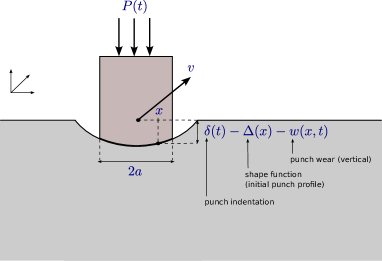
Figure 2.1. Illustration of the geometry of the problem

The first term on the left-hand side of (2.1) accounts for the additional deformation due to the presence of a coating or to model surface roughness [4, 14]. The strength of this effect is measured by the constant $\eta>0$.
The initial punch profile $\Delta\left(x\right)$ is a known function whereas the punch indentation $\delta\left(t\right)$ is a function of only time. Its initial value $\delta\left(0\right)$ can be found from solving

(2.5) $$\eta p\left(x,0\right)+\int_{-a}^{a}K\left(x-\xi\right)p\left(\xi,0\right)\mathrm{d}\xi=\delta\left(0\right)-\Delta\left(x\right),\hskip 10.00002ptx\in\left(-a,a\right),$$

and requiring that $\int_{-a}^{a}p\left(x,0\right)\mathrm{d}x=P_{0}$, as follows from (2.1) and (2.2), respectively, evaluated at $t=0$.
Finally, $w\left[p\right]\left(x,t\right)$ is the wear term which is an operator acting on the contact pressure $p\left(x,t\right)$. Following the discussion in [16, Sec. 3], we take it as

(2.6) $$w\left[p\right]\left(x,t\right)=-\nu\mu^{1/\alpha-1}\int_{0}^{t}\mathcal{E}_{\alpha}\left(\mu^{1/\alpha}\left(t-\tau\right)\right)p\left(x,\tau\right)\mathrm{d}\tau,$$

where $\mu>0$ is a constant and the special function $\mathcal{E}_{\alpha}$ can be defined as

(2.7) $$\mathcal{E_{\alpha}}\left(x\right):=\frac{\alpha}{x}\sum_{k=1}^{\infty}\frac{\left(-1\right)^{k}kx^{\alpha k}}{\Gamma\left(\alpha k+1\right)},\hskip 10.00002ptx>0,\hskip 10.00002pt\alpha>0,$$

with $\Gamma$ being the Gamma function. Note that, in particular case, when $\alpha=1,$we have $\mathcal{E}_{1}\left(x\right)=-\exp\left(-x\right)$.
We will make use of the following asymptotics

(2.8) $$\mathcal{E_{\alpha}}\left(x\right)=-\frac{\alpha}{\Gamma\left(1+\alpha\right)}\frac{1}{x^{1-\alpha}}+\mathcal{O}\left(\frac{1}{x^{1-2\alpha}}\right),\hskip 10.00002pt\hskip 10.00002pt\left|x\right|\ll 1,$$

(2.9) $$\mathcal{E_{\alpha}}\left(x\right)=\begin{cases}-\frac{\alpha}{\Gamma\left(1-\alpha\right)}\frac{1}{x^{\alpha+1}}+\mathcal{O}\left(\frac{1}{x^{2\alpha+1}}\right),&\alpha\in\left(0,1\right)\cup\left(1,2\right),\\ -\exp\left(-x\right),&\alpha=1,\end{cases}\hskip 10.00002pt\hskip 10.00002ptx\gg 1,$$

as well as the integral relation

(2.10) $$\int_{0}^{x_{0}}\mathcal{E}_{\alpha}\left(\lambda^{1/\alpha}x\right)\mathrm{d}x=\lambda^{-1/\alpha}\left[E_{\alpha}\left(-\lambda x_{0}^{\alpha}\right)-1\right],\hskip 10.00002ptx_{0}>0,\hskip 10.00002pt\alpha>0,\hskip 10.00002pt\lambda>0,$$

where $E_{\alpha}$ is the Mittag-Leffler function defined as

(2.11) $$E_{\alpha}\left(z\right):=\sum_{k=0}^{\infty}\frac{z^{k}}{\Gamma\left(\alpha k+1\right)},\hskip 10.00002ptz\in\mathbb{C},\hskip 10.00002pt\alpha>0.$$

In particular, we have $E_{1}\left(z\right)=\exp z$, $z\in\mathbb{C}$, and $E_{\alpha}\left(0\right)=1$, $\alpha>0$. Moreover, the following useful asymptotic holds true

(2.12) $$E_{\alpha}\left(-x\right)=\begin{cases}\frac{1}{\Gamma\left(1-\alpha\right)}\frac{1}{x}+\mathcal{O}\left(\frac{1}{x^{2}}\right),&\alpha\in\left(0,1\right)\cup\left(1,2\right),\\ \exp\left(-x\right),&\alpha=1,\end{cases}\hskip 10.00002pt\hskip 10.00002ptx\gg 1.$$

References for the above mentioned results can be found in [16, Appendix A].

Finally, we recall from [16, Sec. 3] that when $\alpha=1$ and $\mu=0$ (or more precisely, in the limit of $\mu\searrow 0$), the relation (2.6) reduces to what is consistent with the classical Archard’s law [5]:

(2.13) $$w\left[p\right]\left(x,t\right)=-\nu\int_{0}^{t}p\left(x,\tau\right)\mathrm{d}\tau.$$

3. Analysis

The model (2.1)–(2.2) has been rigorously analysed in [16, Sec. 4]. We adapt here a general theory [16, Thm 6] using the result of [16, Prop. 14] valid for the particular form of the kernel function (2.4). Namely, we have the following theorem.

Theorem 1.

Assume that $\mu\geq 0$, $\eta$, $\nu>0$, $\alpha\in\left(0,2\right)$, $a\neq 2$, and $p\left(\cdot,0\right)\in L^{2}\left(-a,a\right)$ solves (2.5) with $K$ given by (2.4) and $\delta\left(0\right)$ such that $\int_{-a}^{a}p\left(x,0\right)\mathrm{d}x=P_{0}$ for some $P_{0}>0$. Suppose $P\left(t\right)$ is as in (2.3) and $w\left[p\right]$ is defined in (2.6). Then, the unique solution $p\in C_{b}\left(\mathbb{R}_{+};L^{2}\left(-a,a\right)\right)$ of (2.1) satisfying (2.2) is given by

(3.1) $$p\left(x,t\right)=\frac{P\left(t\right)}{2a}+\sum_{k=1}^{\infty}d_{k}\left(t\right)\phi_{k}\left(x\right),\hskip 10.00002ptx\in\left(-a,a\right),\hskip 10.00002ptt\geq 0,$$

where

(3.2) $$d_{k}\left(t\right):= d_{k}^{0}\left[1+\frac{\nu}{\mu\left(\eta+\sigma_{k}\right)+\nu}\left(E_{\alpha}\left(-\left(\mu+\frac{\nu}{\eta+\sigma_{k}}\right)t^{\alpha}\right)-1\right)\right]-\frac{l_{k}}{2a\left(\eta+\sigma_{k}\right)}\left(P\left(t\right)-P\left(0\right)\right)$$

$$-\frac{\nu l_{k}}{2a\left(\eta+\sigma_{k}\right)^{2}}\left(\mu+\frac{\nu}{\eta+\sigma_{k}}\right)^{1/\alpha-1}\int_{0}^{t}\mathcal{E}_{\alpha}\left(\left(\mu+\frac{\nu}{\eta+\sigma_{k}}\right)^{1/\alpha}\left(t-\tau\right)\right)\left[P\left(\tau\right)-P\left(0\right)\right]\mathrm{d}\tau,\hskip 10.00002ptk\geq 1,$$

(3.3) $$d_{k}^{0}:=\int_{-a}^{a}p\left(\xi,0\right)\phi_{k}\left(\xi\right)\mathrm{d}\xi,\hskip 10.00002pt\hskip 10.00002ptl_{k}:=\frac{1}{2a}\int_{-a}^{a}\int_{-a}^{a}K\left(\zeta-\xi\right)\phi_{k}\left(\xi\right)\mathrm{d}\zeta\mathrm{d}\xi,\hskip 10.00002ptk\geq 1.$$

Here, $\mathcal{E}_{\alpha}$ and $E_{\alpha}$ are as in (2.7) and (2.11), respectively, whereas $\phi_{k}\in L_{0}^{2}\left(-a,a\right)$, $\sigma_{k}>0$, $k\geq 1$, are normalised eigenfunctions and eigenvalues of the compact self-adjoint operator

(3.4) $$\mathcal{K}_{2}\left[\phi\right]\left(x\right):=\int_{-a}^{a}\left[K\left(x-\xi\right)-\frac{1}{2a}\int_{-a}^{a}\left(K\left(\zeta-x\right)+K\left(\zeta-\xi\right)\right)\mathrm{d}\zeta\right]\phi\left(\xi\right)\mathrm{d}\xi$$

defined on the functional space

(3.5) $$L_{0}^{2}\left(-a,a\right):=\left\{f\in L^{2}\left(-a,a\right):\;\int_{-a}^{a}f\left(x\right)\mathrm{d}x=0\right\}.$$

Proof.

The statement of the theorem is merely a rephrasement of several results from [16]. First of all, it is straightforward (see also [16, Prop. 11]) to verify that the kernel function (2.4) and the exterior load (2.3) satisfy all assumptions of [16, Thm 6]. Then, thanks to [16, Prop. 14], we observe that a form of the solution given by [16, Thm 6] simplifies since $\text{Ker }\mathcal{K}_{2}$, the kernel space of the auxiliary operator $\mathcal{K}_{2}$, is empty. This last part calls for the additional assumption $a\neq 2$ appearing in the formulation. Finally, the fact that $\sigma_{k}>0$ for $k\geq 1$ follows from [16, Prop. 4] and another use of [16, Prop. 14]. ∎

We now proceed with the main goal of the paper. We identify the stationary state and perform long-time behaviour analysis to study qualitative character and speed of the convergence of the solution to this stationary state.

Proposition 2.

Under assumptions of Theorem (1), there exists $\delta_{p}\in C\left(\mathbb{R}_{+};L^{2}\left(-a,a\right)\right)$, $\left\|\delta_{p}\left(\cdot,t\right)\right\|_{L^{2}\left(-a,a\right)}\longrightarrow 0$ as $t\rightarrow+\infty$, such that the solution $p\left(x,t\right)$ to the model (2.1)–(2.2) can be written as

(3.6) $$p\left(x,t\right)=\widetilde{p}_{\infty}\left(x\right)-W_{0}\left(x\right)\cos\left(\omega t-\psi\left(x\right)\right)+\delta_{p}\left(x,t\right)=:p_{\infty}\left(x,t\right)+\delta_{p}\left(x,t\right),$$

where

(3.7) $$\widetilde{p}_{\infty}\left(x\right):=\frac{1}{2a}\left(P_{0}-P_{\Delta}\right)+\sum_{k=1}^{\infty}\left(d_{k}^{0}\frac{\mu\left(\eta+\sigma_{k}\right)}{\mu\left(\eta+\sigma_{k}\right)+\nu}+\frac{P_{\Delta}\mu l_{k}}{2a\left[\mu\left(\eta+\sigma_{k}\right)+\nu\right]}\right)\phi_{k}\left(x\right),$$

(3.8) $$W_{0}\left(x\right):=\left[W_{1}\left(x\right)+W_{2}\left(x\right)\right]^{1/2},\hskip 10.00002pt\hskip 10.00002pt\psi\left(x\right):=\textnormal{sign}\left(W_{2}\left(x\right)\right)\arccos\frac{W_{1}\left(x\right)}{W_{0}\left(x\right)},$$

(3.9) $$W_{1}\left(x\right):=-1+\frac{P_{\Delta}}{2a}\sum_{k=1}^{\infty}\frac{l_{k}}{\eta+\sigma_{k}}\left[\left(\mu+\frac{\nu}{\eta+\sigma_{k}}\right)^{1/\alpha-1}\frac{\nu}{\eta+\sigma_{k}}C_{k}^{c,\omega}+1\right]\phi_{k}\left(x\right),$$

(3.10) $$W_{2}\left(x\right):=\frac{P_{\Delta}}{2a}\sum_{k=1}^{\infty}\frac{\nu l_{k}}{\left(\eta+\sigma_{k}\right)^{2}}\left(\mu+\frac{\nu}{\eta+\sigma_{k}}\right)^{1/\alpha-1}C_{k}^{s,\omega}\phi_{k}\left(x\right),$$

(3.11) $$C_{k}^{c,\omega}:=\int_{0}^{\infty}\mathcal{E}_{\alpha}\left(\left(\mu+\frac{\nu}{\eta+\sigma_{k}}\right)^{1/\alpha}\tau\right)\cos\left(\omega\tau\right)\mathrm{d}\tau,\hskip 10.00002pt\hskip 10.00002ptC_{k}^{s,\omega}:=\int_{0}^{\infty}\mathcal{E}_{\alpha}\left(\left(\mu+\frac{\nu}{\eta+\sigma_{k}}\right)^{1/\alpha}\tau\right)\sin\left(\omega\tau\right)\mathrm{d}\tau.$$

Moreover, we have

(3.12) $$\left\|\delta_{p}\left(\cdot,t\right)\right\|_{L^{2}\left(-a,a\right)}=\mathcal{O}\left(\exp\left(-\left(\mu+\frac{\nu}{\eta+\sigma_{1}}\right)t\right)\right),\hskip 10.00002ptt\gg 1,\hskip 10.00002pt\alpha=1,$$

(3.13) $$\left\|\delta_{p}\left(\cdot,t\right)\right\|_{L^{2}\left(-a,a\right)}=\mathcal{O}\left(\frac{1}{t^{\alpha}}\right),\hskip 10.00002ptt\gg 1,\hskip 10.00002pt\alpha\in\left(0,1\right)\cup\left(1,2\right).$$

Proof.

Plugging (2.3) into (3.2) and employing (2.10), we obtain

$$d_{k}\left(t\right)= d_{k}^{0}-\frac{P_{\Delta}l_{k}}{2a\left(\eta+\sigma_{k}\right)}\left[\cos\left(\omega t\right)-1\right]+\frac{\nu}{\mu\left(\eta+\sigma_{k}\right)+\nu}\left(d_{k}^{0}+\frac{P_{\Delta}l_{k}}{2a\left(\eta+\sigma_{k}\right)}\right)\left[E_{\alpha}\left(-\left(\mu+\frac{\nu}{\eta+\sigma_{k}}\right)t^{\alpha}\right)-1\right]$$

$$-\frac{\nu l_{k}P_{\Delta}}{2a\left(\eta+\sigma_{k}\right)^{2}}\left(\mu+\frac{\nu}{\eta+\sigma_{k}}\right)^{1/\alpha-1}\left[\cos\left(\omega t\right)\int_{0}^{t}\mathcal{E}_{\alpha}\left(\left(\mu+\frac{\nu}{\eta+\sigma_{k}}\right)^{1/\alpha}\tau\right)\cos\left(\omega\tau\right)\mathrm{d}\tau\right.$$

$$\left.-\sin\left(\omega t\right)\int_{0}^{t}\mathcal{E}_{\alpha}\left(\left(\mu+\frac{\nu}{\eta+\sigma_{k}}\right)^{1/\alpha}\tau\right)\sin\left(\omega\tau\right)\mathrm{d}\tau\right].$$

Note that, due to (2.9), the integrals here are converging even when $t\rightarrow+\infty$. Hence, using the definitions in (3.11), we can write

$$\int_{0}^{t}\mathcal{E}_{\alpha}\left(\left(\mu+\frac{\nu}{\eta+\sigma_{k}}\right)^{1/\alpha}\tau\right)\cos\left(\omega\tau\right)\mathrm{d}\tau=C_{k}^{c,\omega}-\int_{t}^{\infty}\mathcal{E}_{\alpha}\left(\left(\mu+\frac{\nu}{\eta+\sigma_{k}}\right)^{1/\alpha}\tau\right)\cos\left(\omega\tau\right)\mathrm{d}\tau,$$

$$\int_{0}^{t}\mathcal{E}_{\alpha}\left(\left(\mu+\frac{\nu}{\eta+\sigma_{k}}\right)^{1/\alpha}\tau\right)\sin\left(\omega\tau\right)\mathrm{d}\tau=C_{k}^{s,\omega}-\int_{t}^{\infty}\mathcal{E}_{\alpha}\left(\left(\mu+\frac{\nu}{\eta+\sigma_{k}}\right)^{1/\alpha}\tau\right)\sin\left(\omega\tau\right)\mathrm{d}\tau.$$

Consequently, we arrive at

(3.14) $$d_{k}\left(t\right)= d_{k}^{0}\frac{\mu\left(\eta+\sigma_{k}\right)}{\mu\left(\eta+\sigma_{k}\right)+\nu}+\frac{l_{k}P_{\Delta}}{2a}\frac{\mu\left(\eta+\sigma_{k}\right)}{\mu\left(\eta+\sigma_{k}\right)+\nu}-\frac{l_{k}P_{\Delta}}{2a}\frac{\nu}{\left(\eta+\sigma_{k}\right)^{2}}\left(\mu+\frac{\nu}{\eta+\sigma_{k}}\right)^{1/\alpha-1}\left(C_{k}^{c,\omega}+1\right)\cos\left(\omega t\right)$$

$$-\frac{l_{k}P_{\Delta}}{2a}\frac{\nu}{\left(\eta+\sigma_{k}\right)^{2}}\left(\mu+\frac{\nu}{\eta+\sigma_{k}}\right)^{1/\alpha-1}C_{k}^{s,\omega}\sin\left(\omega t\right)+r_{k}\left(t\right),$$

where

(3.15) $$r_{k}\left(t\right):= \frac{\nu}{\mu\left(\eta+\sigma_{k}\right)+\nu}\left(d_{k}^{0}+\frac{P_{\Delta}l_{k}}{2a\left(\eta+\sigma_{k}\right)}\right)E_{\alpha}\left(-\left(\mu+\frac{\nu}{\eta+\sigma_{k}}\right)t^{\alpha}\right)$$

$$+\frac{l_{k}P_{\Delta}}{2a}\frac{\nu}{\left(\eta+\sigma_{k}\right)^{2}}\left(\mu+\frac{\nu}{\eta+\sigma_{k}}\right)^{1/\alpha-1}\int_{t}^{\infty}\mathcal{E}_{\alpha}\left(\left(\mu+\frac{\nu}{\eta+\sigma_{k}}\right)^{1/\alpha}\tau\right)\cos\left(\omega\left(t-\tau\right)\right)\mathrm{d}\tau.$$

Substitution of (3.14) into (3.1) and taking into account (3.7)–(3.10) yields (3.6) with

(3.16) $$\delta_{p}\left(x,t\right):=\sum_{k=1}^{\infty}r_{k}\left(t\right)\phi_{k}\left(x\right).$$

It now remains to deduce (3.12)–(3.13). To this effect, we first note that, due to the mutual orthogonality of functions $\left\{\phi_{k}\right\}_{k=1}^{\infty}$, we have

(3.17) $$\left\|\delta_{p}\left(\cdot,t\right)\right\|_{L^{2}\left(-a,a\right)}=\left(\sum_{k=1}^{\infty}\left|r_{k}\left(t\right)\right|^{2}\right)^{1/2}.$$

Using the fact that $0<\sigma_{k}\leq\sigma_{k-1}$ for $k>1$, we can estimate, for sufficiently large $t>0$,

(3.18) $$\left(\sum_{k=1}^{\infty}\left|\frac{\nu}{\mu\left(\eta+\sigma_{k}\right)+\nu}E_{\alpha}\left(-\left(\mu+\frac{\nu}{\eta+\sigma_{k}}\right)t^{\alpha}\right)d_{k}^{0}\right|^{2}\right)^{1/2}$$

$$\leq\frac{\nu}{\mu\eta+\nu}\left|E_{\alpha}\left(-\left(\mu+\frac{\nu}{\eta+\sigma_{1}}\right)t^{\alpha}\right)\right|\left\|p_{0}\left(\cdot,t\right)\right\|_{L^{2}\left(-a,a\right)},$$

(3.19) $$\left(\sum_{k=1}^{\infty}\left|\frac{P_{\Delta}\nu}{2a\left(\eta+\sigma_{k}\right)\left[\mu\left(\eta+\sigma_{k}\right)+\nu\right]}E_{\alpha}\left(-\left(\mu+\frac{\nu}{\eta+\sigma_{k}}\right)t^{\alpha}\right)l_{k}\right|^{2}\right)^{1/2}$$

$$\leq\frac{P_{\Delta}\nu}{2a\eta\left(\mu\eta+\nu\right)}\left|E_{\alpha}\left(-\left(\mu+\frac{\nu}{\eta+\sigma_{1}}\right)t^{\alpha}\right)\right|\left\|K_{1}\right\|_{L^{2}\left(-a,a\right)},$$

with

$$K_{1}\left(x\right):=\int_{-a}^{a}K\left(\zeta-x\right)\mathrm{d}\zeta=2a\left(1+C_{K}\right)-\left(a+x\right)\log\left(a+x\right)-\left(a-x\right)\log\left(a-x\right).$$

Here, we employed the Parseval’s identity $\sum_{k=1}^{\infty}\left|d_{k}^{0}\right|^{2}=\left\|p\left(\cdot,0\right)\right\|_{L^{2}\left(-a,a\right)}^{2}$, $\sum_{k=1}^{\infty}\left|l_{k}\right|^{2}=\left\|K_{1}\right\|_{L^{2}\left(-a,a\right)}^{2}$ and the fact that $E_{\alpha}\left(-t\right)$ is a monotonous function for sufficiently large values of $t$ (as follows from (2.9)).

Then, thanks to the triangle inequality for the Euclidean $l^{2}$ norm, we estimate (3.17) using (3.15) and (3.18)–(3.19) as

(3.20) $$\left\|\delta_{p}\left(\cdot,t\right)\right\|_{L^{2}\left(-a,a\right)}\leq \frac{\nu}{\mu\eta+\nu}\left[\left\|p\left(\cdot,0\right)\right\|_{L^{2}\left(-a,a\right)}+\frac{P_{\Delta}}{2a\eta}\left\|K_{1}\right\|_{L^{2}\left(-a,a\right)}\right]\left|E_{\alpha}\left(-\left(\mu+\frac{\nu}{\eta+\sigma_{1}}\right)t^{\alpha}\right)\right|$$

$$+\frac{P_{\Delta}\nu}{2a\eta^{2}}\left\|K_{1}\right\|_{L^{2}\left(-a,a\right)}\sup_{k\geq 1}\left(\mu+\frac{\nu}{\eta+\sigma_{k}}\right)^{1/\alpha-1}\left|\int_{t}^{\infty}\mathcal{E}_{\alpha}\left(\left(\mu+\frac{\nu}{\eta+\sigma_{k}}\right)^{1/\alpha}\tau\right)\cos\left(\omega\left(t-\tau\right)\right)\mathrm{d}\tau\right|.$$

In case $\alpha=1$, the functions $E_{\alpha}$ and $\mathcal{E}_{\alpha}$ in (3.20) reduce to exponential functions. Employing the simple result

$$\int_{t}^{\infty}e^{-\beta_{k}\tau}\cos\left(\omega\left(t-\tau\right)\right)\mathrm{d}\tau=\frac{\beta_{k}e^{-\beta_{k}t}}{\beta_{k}^{2}+\omega^{2}}$$

with $\beta_{k}:=\left(\mu+\frac{\nu}{\eta+\sigma_{k}}\right)^{1/\alpha}$, we have

$$\sup_{k\geq 1}\left(\mu+\frac{\nu}{\eta+\sigma_{k}}\right)^{1/\alpha-1}\left|\int_{t}^{\infty}\mathcal{E}_{\alpha}\left(\left(\mu+\frac{\nu}{\eta+\sigma_{k}}\right)^{1/\alpha}\tau\right)\cos\left(\omega\left(t-\tau\right)\right)\mathrm{d}\tau\right| \leq\sup_{k\geq 1}\frac{\beta_{k}^{2-\alpha}e^{-\beta_{k}t}}{\beta_{k}^{2}+\omega^{2}}$$

$$\leq e^{-\beta_{1}t},$$

and thus deduce (3.12).

In case $\alpha\in\left(0,1\right)\cup\left(1,2\right)$, we first use (2.12) in the first line of (3.20) to deduce the $\mathcal{O}\left(1/t^{\alpha}\right)$ decay of the corresponding term. Next, we estimate

$$\left(\mu+\frac{\nu}{\eta+\sigma_{k}}\right)^{1/\alpha-1}\left|\int_{t}^{\infty}\mathcal{E}_{\alpha}\left(\left(\mu+\frac{\nu}{\eta+\sigma_{k}}\right)^{1/\alpha}\tau\right)\cos\left(\omega\left(t-\tau\right)\right)\mathrm{d}\tau\right|\leq\frac{C_{\alpha}}{\alpha}\frac{1}{t^{\alpha}},$$

which is due to the finiteness of the constant $C_{\alpha}:=\sup_{\tau>0}\tau^{1+\alpha}\left|\mathcal{E}_{\alpha}\left(\tau\right)\right|$ entailed by the continuity of $\mathcal{E}_{\alpha}$ (away from $t=0$) and asymptotics (2.8)–(2.9). Therefore, the decay result (3.13) follows. ∎

4. Numerical illustrations

We fix the following set of parameters $a=1$, $\nu=2$, $\eta=1$, $\mu=1.2$, $C_{K}=\log 5\simeq 1.61$. We take the oscillatory load profile (2.3) with $P_{0}=6$, $P_{\Delta}=0.5$, $\omega=1.5$. For simplicity, we assume that the punch profile $\Delta\left(x\right)$ is such that

(4.1) $$p\left(x,0\right)=\frac{2P_{0}}{a^{2}\pi}\sqrt{a^{2}-x^{2}},\hskip 10.00002ptx\in\left(-a,a\right),$$

which is a reasonable initial pressure form.

All computations are performed using $60$ terms in the expansion (3.1).

We illustrate the results for 3 different values of the parameter $\alpha$ ($\alpha\in\left\{0.8,1.0,1.8\right\}$) with the parameter $\mu=1.2$ and again with $\mu=0$. In the latter case, the model is purely of a fractional order (no relaxation effect). Also, recall that when $\alpha=1$, the model reduces to that which does not involve fractional calculus (with or without relaxation, depending on $\mu$).

In Figure 4.1, we plot the stationary state pressure profile (or, more precisely, a collection of curves $p_{\infty}\left(\cdot,t\right)$ evaluated for $t\in\left[0,2\pi/\omega\right]$) and investigate the dependence of its envelope (given by $\widetilde{p}_{\infty}\pm W_{0}$) on the choice of model parameters $\alpha$ and $\mu$. Evidently, for $\mu=1.2$ the impact of the parameter $\alpha$ on the stationary state is almost undetectable, which is not the case when $\mu=0$.

Figure 4.2 shows the character and the speed of convergence of the solution to the stationary state $p_{\infty}$ measured by the quantity $\left\|\delta_{p}\left(\cdot,t\right)\right\|_{L^{\infty}\left(-a,a\right)}:=\left\|p\left(\cdot,t\right)-p_{\infty}\left(\cdot,t\right)\right\|_{L^{\infty}\left(-a,a\right)}$. Since the initial profile (4.1) is bounded, the pressure values at larger times are expected to remain bounded too. This is why we replaced the $L^{2}$ norm with the $L^{\infty}$ norm in visualising the solution convergence. Clearly, the results are in direct correspondence to the analytical prediction given by (3.12)–(3.13).

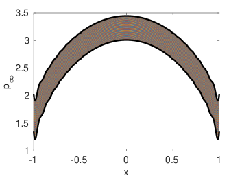
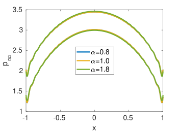
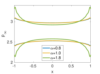
Figure 4.1. Stationary state $p_{\infty}\left(x,t\right)$ for multiple values of $t$ over the period $T=2\pi/\omega\simeq 4.19$ with $\mu=1.2$ (above) and its envelope for 3 different values of $\alpha$ (below) with $\mu=1.2$ (left) and $\mu=0$ (right)

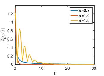
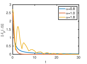
Figure 4.2. Convergence of the solution to the stationary state for 3 different values of $\alpha$
with $\mu=1.2$ (left) and $\mu=0$ (right)

5. Discussion and conclusion

We have revisited the classical sliding punch problem with a recently proposed generalised model of wear. In particular, we have investigated long-time evolution of the pressure profile under a practically important case of exterior time-harmonic load. We have derived an explicit form of the stationary pressure distribution in terms of eigenfunctions of an auxiliary integral operator. Moreover, we have analysed a speed of the convergence of the model solution to this distribution. We note that, in contrast to previous results when the load was constant (or eventually constant, see [16, Sec. 5]), here the stationary distribution $p_{\infty}$ is a function of both space and time. Its time dependence is, nevertheless, clear and structurally simple: it is harmonic with the same frequency as the exterior load but with a phase shift that depends on the spatial variable (see (3.6)).

Numerical simulations have been performed to illustrate the obtained results. In particular, the focus was on the dependence of the mentioned results on the parameters $\alpha$, $\mu$ which are characteristic for the present model. It is remarkable that the dependence of the stationary state on the model order $\alpha$ is insignificant when $\mu\neq 0$. The parameter $\alpha$, however, has an essential impact on the speed of the convergence towards the stationary state: the convergence is exponential for $\alpha=1$, whereas for $\alpha\in\left(0,1\right)\cup\left(1,2\right)$, it is algebraic but its rate grows with the increase of $\alpha$. Moreover, when $\alpha\in\left(1,2\right)$ the convergence happens in a non-monotone fashion. The similar effect of $\alpha$ on the convergence rate was observed in the previous work [16] when the load was constant or eventually constant. We thus confirm here the previous observation that the model parameters $\mu$ and $\alpha$ affect essentially the stationary state profile and the speed of convergence, respectively. These statements would constitute important guidelines when trying to fit the new model to experimental data. Such a fit would be essential for a practical validation of the model.

References

• [1] Alblas, J. B., Kuipers, M.: Contact problems of a rectangular block on an elastic layer of finite thickness: the thin layer. Acta Mech., 8 (3), 133–145 (1969).
• [2] Alblas, J. B., Kuipers, M.: Contact problems of a rectangular block on an elastic layer of finite thickness: the thick layer. Acta Mech., 9 (1), 1–12 (1970).
• [3] Aleksandrov, V. M., Kovalenko, E. V.: Mathematical methods in problems with wear (in Russian). Nonlinear Models and Problems of Mechanics of Solids, Contributions edited by K. V. Frolov (1984).
• [4] Aleksandrov, V. M., Kovalenko, E. V.: On the theory of contact problems in the presence of nonlinear wear (in Russian). Mech. Solids. 4, 98–108 (1982).
• [5] Archard, J. F.: Contact and Rubbing of Flat Surfaces. Journal of Applied Physics 24, 981 (1953).
• [6] Argatov, I. I.: A Fractional Time-Derivative Model for Severe Wear: Hypothesis and Implications. Frontiers in Mechanical Engineering, 8 (2022).
• [7] Argatov, I. I., Chai, Y. S.: Effective wear coefficient and wearing-in period for a functionally graded wear-resisting punch. Acta Mech. 230, 2295–2307 (2019).
• [8] Argatov, I. I., Chai, Y. S.: Wear contact problem with friction: Steady-state regime and wearing-in period. Int. J. Sol. Struct. 193–194, 213–221 (2020).
• [9] Argatov, I. I., Fadin, Yu. A.: A Macro-Scale Approximation for the Running-In Period. Tribol. Lett. 42, 311–317 (2011).
• [10] Feppon, F., Sidebottom, M. A., Michailidis, G., Krick, B. A., Vermaak, N.: Efficient steady-state computation for wear of multimaterial composites. Journal of Tribology, 138 (3), 2016.
• [11] Galin L. A.: Contact problems of the theory of elasticity in the presence of wear. J. Appl.Math. Mech. 40 (6), 931–936, 1976.
• [12] Gorenflo, R., Mainardi, F.: Fractional Calculus: Integral and Differential Equations of Fractional Order. arXiv:0805.3823, 56 pp. (2008).
• [13] Goryacheva, I. G.: Contact Mechanics in Tribology. Springer (1998).
• [14] Kovalenko, E. V.: On an efficient method of solving contact problems with linearly deformable base with a reinforcing coating (in Russian). Mechanics. Proceedings of National Academy of Sciences of Armenia 32 (2), 76–82 (1979).
• [15] Komogortsev, V. F.: Contact between a moving stamp and an elastic half-plane when there is wear. J. Appl. Maths Mechs 49, 243–246 (1985).
• [16] Ponomarev, D.: A generalised time-evolution model for contact problems with wear and its analysis, arXiv:2203.03066 (2022).
• [17] Samko, S. G., Kilbas, A. A., Marichev, O. I.: Fractional Integrals and Derivatives - Theory and Applications. Gordon and Breach Science Publishers (1993).
• [18] Vorovich I. I, Aleksandrov, V. M., Babeshko, V. A.: Non-classical mixed contact problems in elasticity theory (in Russian). Nauka (1974).
• [19] Yevtushenko, A. A., Pyr’yev, Yu. A.: The applicability of a hereditary model of wear with an exponential kernel in the one-dimensional contact problem taking frictional heat generation into account. J. Appl. Maths Mechs 63 (5), 795–801 (1996).
• [20] Zhu, D., Martini, A., Wang, W., Hu, Y., Lisowsky, B., Wang, Q. J.: Simulation of Sliding Wear in Mixed Lubrication. ASME. J. Tribol. 129 (3), 544–552 (2007).