Enhanced spin-mechanical interaction with levitated micromagnets

Abstract

Spin-mechanical hybrid systems have been widely used in quantum information processing. However, the spin-mechanical interaction is generally weak, making it a critical challenge to enhance the spin-mechanical interaction into the strong coupling or even ultra-strong coupling regime. Here, we propose a protocol that can significantly enhance the spin-mechanical coupling strength with a diamond spin vacancy and a levitated micromagnet. A driving electrical current is used to modulate the mechanical motion of the levitated micromagnet, which induces a two-phonon drive and can exponentially enhance the spin-phonon and phonon-medicated spin-spin coupling strengths. Furthermore, a high fidelity Schrödinger cat state and an unconventional 2-qubit geometric phase gate with high fidelity and faster gate speed can be achieved using this hybrid system. This protocol provides a promising platform for quantum information processing with NV spins coupled to levitated micromagnets.

I introduction

Hybrid quantum systems, which combine the advantages of various quantum systems to overcome their shortcomings, have been widely used in quantum information processing [1, 2, 3]. Several proposals for hybrid systems in cavity-QED [4], circuit-QED [5], and spin-mechanical hybrid systems [6, 7, 8, 9, 10, 11, 12, 13, 14, 15, 16, 17, 18, 19, 20, 21, 22, 23, 24, 25, 26, 27, 28, 29] have already been implemented in recent years. The spin-mechanical hybrid system combines quantum systems with long coherence time, such as trapped atoms or ions [30, 31, 32, 33, 34], solid-state spins [35, 36, 37, 38, 39, 40, 41], and mechanical oscillators with high-quality factors, such as cantilevers [17, 16, 23, 22, 21, 18, 20, 19] and nanobeams [14, 12, 13, 11]. It has been widely used in the preparation of a non-classical quantum state of mechanical motion [25, 24], ground-state cooling [16, 14, 15], ultrasensitive sensing [10, 42], as well as the generation of interaction between two distant quantum systems [20, 18, 19, 17]. The greatest impediment to its possible applications is the unavoidable dissipation of the oscillators interacting with the environment. To reduce dissipation, researchers have developed levitated devices [43, 44, 45, 46, 47, 48, 49, 50, 51, 52, 53, 54, 55, 56, 57, 58, 59, 60, 61, 62, 63, 64, 65, 66, 67, 64] that readily isolated the oscillators from the environment.

Optical, electrical, and magnetic levitation are the three types of suspending setups that can all work in a vacuum environment. The magnetic trap with a passive field [43, 44, 51, 52, 53, 50, 49, 55, 54, 48, 47, 46, 56, 45] is simpler than the optical trap with lasers [60, 59, 57, 58] and the electrical trap with radio-frequency modulation of a high voltage electric field [32, 31, 34, 33]. Photon recoil, damage to suspended particles caused by the laser’s thermal effect, and clamping losses can all be avoided via magnetostatic field levitation [56]. For these suspended schemes, the suspension objectives are diverse. Glass spheres [59], superconductor spheres [62], superconductor rings [46, 67], magnetic microspheres [43, 42], silicon particles [58, 64] and diamond particles [56, 57, 54, 55] have all been investigated on various platforms. Because of their isolation, they have been used to construct ultra-sensitive sensors [43, 42] as well as to couple superconducting circuits [48] and solid-state spins [15, 34, 64]. Magnetic microspheres, particularly YIG (yttrium iron garnet) spheres due to their high spin density [68], have received a great attention [69, 70, 71, 72, 73, 74, 75, 76, 77]. There have been investigations on magnon coupling to cavity modes such as a sphere cavity [72], co-axis cavity [73], 3D cavity [74], and so on. Classical Rabi-like oscillation [75], magnetically induced transparency [75], bistable states [76], and other intriguing quantum effects have been observed. Furthermore, the YIG sphere can couple to microwave photons and solid-state spins, which has been utilized to improve the coupling strength between a solid-state spin and a photon mode [77]. In addition, the levitated micromagnets coupled to solid-state spins have been studied [51]. Recent study has showed the interaction of a nitrogen-vacancy (NV) center in diamond with a levitated micromagnet through the magnetic field gradient produced by the micromagnet [51]. The coupling strength, however, is so weak that it can not be used for quantum information tasks.

Inspired from previous experimental and theoretical progress, we propose a useful approach to exponentially enhance the spin-mechanical coupling strength in a spin-magnetomechanical system. An NV center is situated near the hard spherical micromagnet, which levitates above a type-II superconductor. The magnetic field gradient generated by the micromagnet couples the NV center to the center-of-mass motion of the micromagnet. Many schemes have been proposed to enhance the single-quantum interaction on various platforms. Nonlinear resources [78, 79, 80, 81, 82] and parametric drive [83, 84] (for example, two-photon drive) have been utilized to increase light-matter interactions. The modulation of voltage in a trapped-ion system is used to achieve parametric amplification [85, 86, 87]. Modulating the spring constant of a cantilever [88] increases the spin-phonon coupling strength exponentially in a spin-mechanical system [17]. This work suggests a classical electrical-current-driven approach for achieving exponential enhancement of spin-mechanical interactions in a suspended micromagnet platform. The driving current is located above the levitated micromagnet. The trap potential is modified by the magnetic field of the current, which modulates the oscillation frequency of the micromagnet’s mechanical motion. This modulation process can provide a two-phonon drive capable of amplifying the mechanical zero-point fluctuations, hence increasing the spin-mechanical interaction. In other words, despite merely employing a classical drive current, we obtain a nonlinear resource and, as a consequence, achieve the strong coupling regime without adding any nonlinear sources into the system. Utilizing the strongly coupled spin-mechanical system, one can prepare a high fidelity superposition state of the levitated micromagnet. In addition, the phonon-mediated spin-spin coupling can be obtained when two NV centers are coupled to the same mechanical oscillator [18, 20, 19, 17], and the interaction can also be exponentially amplified with a driving current. With the enhanced spin-spin coupling, the two-NV protocol can also construct an unconventional 2-qubit geometric phase gate with the property of high fidelity, shorter operation time, and universality.

II Setup and protocol

II.1 The setup

Fig. 1(a) presents a hybrid system that includes a micromagnet, an NV center, and a driving current. The hard spherical micromagnet with radius $a$, mass $m$, levitates on the type-II superconductor because of the flux trapping effect, the superconductor freezing or trapping the magnetic flux that penetrates it during the cooldown (see Fig. 1(a)) [51, 89, 63]. The microfabricated pocket provides a stable vacuum environment to isolate the micromagnet from the environment, enabling the dissipation of the system to be decreased. A cosine-function drive is provided by the current above the micromagnet, and the NV center is placed nearby the micromagnet. Fig. 1(b) depicts the principle of this setup. The micromagnet trapped in the magnetostatic field, which can be calculated via the frozen dipole model (Fig. 1(c)), can be compared to a simple harmonic oscillator that couples to the NV center. The NV center transition (Fig. 1(d)) is driven by a linearly polarized microwave in the $y$-direction, and the transverse static magnetic field (i.e. $x$-direction) results in a mix of the eigenstates of $\hat{\sigma}_{z}$. The energy level structure of the mixed states is depicted in Fig. 1(e). Fig. 1(f) presents the energy level splitting of the mixed states varying with the $x$-direction magnetic field.

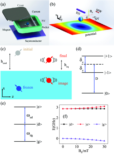
Figure 1: Setup sketch: (a) the model of our proposal. (b) shows the principle of our setup. (c) displays the frozen dipole model. (d) the energy level structure of NV centers. It will produce the Zeeman splitting when a $z$-direction magnetic field is applied. (e) the energy level structure of the mixed states. (f) the energy level splitting of the mixed states varys with the $x$-direction magnetic field.

II.2 Levitation of the micromagnet

As shown in Fig. 1(b), the position of the levitated micromagnet with mass $m$ and radius $a$ in the direction of gravity is represented by $x$. The acceleration of gravity is $g=9.8m/s^{2}$. According to the frozen dipole model [89], the effective magnetic field $\bm{B_{eff}}$ at the position of the levitated micromagnet consists of the magnetic field $\bm{B_{f}}$ generated by frozen dipole and the magnetic field $\bm{B_{i}}$ generated by image dipole, as depicted in Fig. 1(c). Then the potential energy of the levitated micromagnet is given by

$$U=\bm{-\mu\cdot B_{eff}}+mgx,$$ (1)

where the $\bm{B_{eff}}=\bm{B_{f}}+1/2\bm{B_{i}}$ is the effective magnetic field produced by the interaction between the micromagnet and type-II superconductor [51]. We can derive an analytic formula for the potential energy $U$ as

$$U=U_{s}\left(\alpha_{s}x_{s}+g_{u}\right),$$ (2)

where $l_{s}=l/a$ ($l=x,y,z$), $\alpha_{s}=a/\alpha_{crit}$, $U_{s}=mg\alpha_{crit}$, and $\alpha_{crit}=B_{r}^{2}/(16g\rho\mu_{0})$. $B_{r}$, $\rho$, and $\mu_{0}$ are residual flux density, density of the micromagnet, and vacuum permeability. The dimensionless potential energy defined by $u_{s}=\alpha_{s}x_{s}+g_{u}$ in Eq. (2) is plotted in Fig. 2, showing that the micromagnet can be steadily trapped in the potential trap. Fig. 2(a), (b), and (c) present the dimensionless potential energy $u_{s}$ of the micromagnet in the $zy$-plane, $zx$-plane, and $\theta\phi$-plane, respectively. In the $zy$-direction, the potential energy exhibits strong symmetry. As depicted in Fig. 2(c), the equilibrium orientation of the levitation micromagnet $\theta$ and $\phi$ is, interestingly, the same as the initial orientation $\theta_{cool}$ and $\phi_{cool}$. It means that the rotation of the micromagnet can be neglected, or that the ultimate orientation can be set as $\theta=\theta_{cool}=0$, $\phi=\phi_{cool}=\pi/2$. The potential energy distribution along the $z$-axis illustrated in Fig. 2(d) can be well approximated as a harmonic potential, implying that the motion of the micromagnet is harmonic. In addition, the levitated micromagnet provides a strong magnetic field gradient for spin-mechanical coupling.

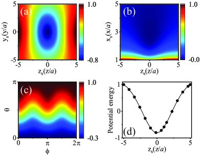
Figure 2: The potential energy of the levitated micromagnet. The dimensionless potential energy $u_{s}$ in $zy$-plane, $zx$-plane, $\theta\phi$-plane and $z$-direction are shown in (a), (b), (c), and (d), respectively. Here, the radius and the density of the micromagnet are $a=22.4\mu m$ and $\rho=7430kg/m^{3}$, respectively. The initial position and the equilibrium position are both $3a$. The initial orientation is $\phi_{cool}=\pi/2$ and $\theta_{cool}=0$. And residual induction is $B_{r}=750mT$.

II.3 Hamiltonian of the system

The NV center is coupled to the micromagnet in this protocol through the magnetic field gradient induced by the micromagnet in the $z$-direction. In the presence of a homogeneous static magnetic field in the $x$-direction $\bm{B_{s}}=B_{0}\bm{\hat{e}_{x}}$, the ground state Hamiltonian of the NV center can be written as $\hat{H}_{NV}=D\hat{S}_{z}^{2}+\gamma_{e}\bm{\hat{S}\cdot B_{s}}$, where $\gamma_{e}=g_{e}\mu_{B}$ is the electron gyromagnetic factor and $D/2\pi=2.87$ GHz is the zero-field splitting between sublevel $|m_{s}=0\rangle$ and $|m_{s}=\pm 1\rangle$ (see Fig. 1(d)). $g_{e}\simeq 2$ and $\mu_{B}=14$MHz/mT are the Landaé factor of electron and Bohr magneton, respectively. $\bm{\hat{S}}$ is electron spin operator including the components $\hat{S}_{x}$, $\hat{S}_{y}$, and $\hat{S}_{z}$. The microwave (MW) drive $B_{y}(t)=B_{y}^{0}\cos\omega_{p}t$ polarized in the $y$-direction is applied to drive the transition between the sublevels, where $B_{y}^{0}$ and $\omega_{p}$ are the amplitude and the microwave frequency of the drive respectively. Then the Hamiltonian is given by

$$\hat{H}_{NV}=D\hat{S}_{z}^{2}+\delta\hat{S}_{x}+\Omega_{p}{\rm cos}\left(\omega_{p}t\right)\hat{S}_{y},$$ (3)

where $\Omega_{p}=\gamma_{e}B_{y}^{0}$ is the Rabi frequency and $\delta=\gamma_{e}B_{0}$.

The motion of a levitated micromagnet can be regarded as three independent harmonic motions in three directions around the equilibrium position. Only the harmonic motion of the $z$-direction, which is the same as the spin direction of the NV center, is considered here. Its Hamiltonian is

$$\hat{H}_{ma}=\frac{\hat{p}_{z}^{2}}{2m}+\frac{1}{2}k_{ma}\hat{z}^{2}$$ (4)

with

$$k_{ma}=\frac{3\mu_{0}\mu_{m}^{2}}{4\pi(h_{eq}+h_{cool})^{5}},$$ (5)

where $\hat{p}_{z}$ and $\hat{z}$ are the momentum and position operators, respectively, and $\mu_{m}$ is the magnetic moment of the micromagnet. $h_{eq}$ and $h_{cool}$ represent the initial position and equilibrium position of the micromagnet respectively. The trapping frequency of the levitated micromagnet is defined by $\omega_{ma}=\sqrt{k_{ma}/m}$, which is related to the cooling down conditions. With $\hat{p}_{z}=-i\sqrt{m\omega_{ma}/2}(\hat{a}-\hat{a}^{\dagger})$, $\hat{z}=z_{0}(\hat{a}+\hat{a}^{\dagger})$, and zero-point fluctuation $z_{0}=\sqrt{1/(2m\omega_{ma})}$, we can simplify the Hamiltonian of the micromagnet. The result is

$$\hat{H}_{ma}=\omega_{ma}\hat{a}^{\dagger}\hat{a},$$ (6)

The interaction between the NV center and the micromagnet will be the subject of our next discussion. The micromagnet can be described as a magnetic dipole in classical electrodynamics, with

$$\bm{B}=\frac{\mu_{0}}{4\pi}\left[\frac{3\bm{r}(\bm{\mu}\cdot\bm{r})}{r^{5}}-\frac{\bm{\mu}}{r^{3}}\right]$$ (7)

describing the magnetic field surrounding it. Only the magnetic field in the $z$-direction is concerned here, which is given by $\bm{B}=2\mu_{0}\mu_{m}\bm{\hat{e}_{z}}/[4\pi(d-z)^{3}]$. The magnetic field is represented by

$$\bm{B}\simeq\frac{2\mu_{0}\mu_{m}\bm{\hat{e}_{z}}}{4\pi d^{3}}+\frac{3\mu_{0}\mu_{m}\hat{z}\bm{\hat{e}_{z}}}{4\pi d^{4}}+O(\hat{z}^{2})$$ (8)

around the equilibrium position. After removing the high order and constant components, and quantizing the motion (more details in Appendix B), the interaction Hamiltonian is expressed as

$$\hat{H}_{int}=\lambda(\hat{a}+\hat{a}^{\dagger})\hat{S}_{z},$$ (9)

where $\lambda=\gamma_{e}B_{r}a^{3}z_{0}/d^{4}$ is the coupling strength and $d$ is the distance between the NV center and the micromagnet.

Finally, $I_{cu}=I_{0}{\rm cos}2\omega_{cu}t$ is the drive current placed above the micromagnet, where $\omega_{cu}$ is the driving current frequency and $I_{0}$ is the amplitude of the driven electrical current. The Hamiltonian of the driving current is given by $\hat{H}_{cu}=1/2k_{cu}^{2}\hat{z}^{2}{\rm cos}2\omega_{cu}t$. After quantization (Appendix C), we can have

$$\hat{H}_{cu}=-g_{cu}(\hat{a}+\hat{a}^{\dagger})^{2}{\rm cos}2\omega_{cu}t,$$ (10)

where $g_{cu}=k_{cu}z_{0}^{2}/2$ defines the coupling strength between the driving current and the micromagnet. The nonlinear term or the parametric amplification is obtained by the linear drive. The spin-mechanic coupling strength can be exponentially enhanced with such a nonlinear term, as demonstrated below.

III enhancing the coupling strength

III.1 One NV

Based on the foregoing analysis, the total Hamiltonian of the hybrid system is

$$\hat{H}_{TO}=\hat{H}_{NV}+\hat{H}_{ma}+\hat{H}_{int}+\hat{H}_{cu}.$$ (11)

The first term is the Hamiltonian of NV centers. The second corresponds to the free Hamiltonian of the micromagnet, the third describes the interaction between the NV center and micromagnet, and the last is the drive-current Hamiltonian. In the absence of the microwave drive, the Hamiltonian $\hat{H}_{NV}$ is given by

$$\hat{H}_{NV}=D\hat{S}_{z}^{2}+\delta\hat{S}_{x}.$$ (12)

The eigenstates of Eq. (12) are mixed states $|e\rangle={\rm sin}\theta|0\rangle+{\rm cos}\theta|b\rangle$, $|g\rangle={\rm cos}\theta|0\rangle-{\rm sin}\theta|b\rangle$, and $|d\rangle=\left(|+1\rangle-|-1\rangle\right)/\sqrt{2}$, where $|b\rangle=\left(|-1\rangle+|+1\rangle\right)/\sqrt{2}$ and ${\rm tan}2\theta=2\delta/D$, corresponding to the eigenenergy $\omega_{e/g}=D[1\pm\sqrt{1+(2\delta/D)^{2}}]/2$, and $\omega_{d}=D$.

We assume that the microwave is solely used to drive the transition between the mixed states $|g\rangle$ and $|d\rangle$, i.e. $\omega_{p}\simeq\omega_{d}-\omega_{g}=\omega_{dg}$. Transforming to the frame at the microwave frequency and using the rotating-wave approximation, the Hamiltonian in the basis $|e,d,g\rangle$ of the NV center can be reduced as

$$\hat{H}_{NV}=\left(\begin{array}[]{ccc}-\frac{\Delta}{2}&0&0\\ 0&\frac{\Delta}{2}&0\\ 0&0&\omega_{e}^{\prime\prime}\end{array}\right)+\frac{1}{2i}\left(\begin{array}[]{ccc}0&-\Omega_{p}^{\prime}&0\\ \Omega_{p}^{\prime}&0&0\\ 0&0&0\end{array}\right),$$ (13)

where $\Delta=\omega_{p}-\omega_{dg}$, $\omega_{e}^{\prime\prime}=\omega_{e}-(\omega_{d}+\omega_{g}+\omega_{p})/2$, and $\Omega_{p}^{\prime}=\Omega_{p}cos\theta$. We consider a new basis for further diagonalization, consisting of the eigenstates of Eq. (13), which are $|e\rangle$, $|+\rangle=i\sin\alpha|g\rangle+{\cos}\alpha|d\rangle$, and $|-\rangle=-i{\cos}\alpha|g\rangle+{\sin}\alpha|d\rangle$, with eigenenergies $\omega_{e}^{\prime\prime}$ and $\omega_{\pm}=\pm\sqrt{\Delta^{2}+\Omega_{p}^{\prime 2}}/2$, where ${\tan}2\alpha=\Omega_{p}^{\prime}/\Delta$. Using the new eigen basis ${|e,\pm\rangle}$ and the unitary transformation $U={\rm exp}(-i\hat{H}_{u}t)$ with $\hat{H}_{u}=\omega_{cu}(\hat{\sigma}_{z}/2+\hat{a}^{\dagger}\hat{a})$, the Hamiltonian of the hybrid system is represented as

$$\hat{H}_{TO}=\frac{\delta_{0}}{2}\hat{\sigma}_{z}+\delta_{m}\hat{a}^{\dagger}\hat{a}+\Lambda\left(\hat{a}\hat{\sigma}^{+}+\hat{a}^{\dagger}\hat{\sigma}^{-}\right)$$ (14)

$$-\frac{g_{cu}}{2}\left(\hat{a}^{2}+\hat{a}^{\dagger^{2}}\right),$$

where $\hat{\sigma}_{z}\equiv|e\rangle\langle e|-|+\rangle\langle+|$, $\hat{\sigma}_{x}=\hat{\sigma}_{+}+\hat{\sigma}_{-}$, $\hat{\sigma}_{+}\equiv|e\rangle\langle+|$, $\hat{\sigma}_{-}\equiv|+\rangle\langle e|$, $\delta_{0}=\omega_{0}-\omega_{cu}$, $\omega_{0}=\omega_{e}^{\prime\prime}-\omega_{+}$, and $\delta_{m}=\omega_{ma}-\omega_{cu}$. Here only the states $|m,+\rangle$ and $|n,e\rangle$ are resonant with the condition $\left\lvert m-n\right\rvert=1$, $m$ and $n$ being the phonon numbers (see Fig. 3(a)). Under the aforesaid resonant condition, the spin-phonon coupling strength is given by $\Lambda=\lambda{\rm cos}\theta{\rm cos}\alpha$, which is related to the transverse magnetic field $B_{0}$ and $\alpha$, dependent on the microwave frequency $\Omega_{p}^{\prime}$ and $\Delta$, as shown in Fig. 3(b). The coupling strength increases as $B_{0}$ and $\alpha$ decrease, showing that we should choose an appropriate value to make the system work well.

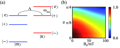
Figure 3: Spin-phonon coupling. (a) shows couplings between the spin and phonons. The intensity of the spin-phonon coupling as a function of $\alpha$ and the transverse static magnetic field $B_{0}$ is shown in (b).

Using the Bogoliubov transformation [83, 90, 87] $\hat{b}=\hat{a}^{\dagger}{\rm cosh}r-\hat{a}{\rm sinh}r$, with ${\rm tanh}2r=g_{cu}/\delta_{m}$, the total Hamiltonian can be expressed in a simple form

$$\hat{H}_{TO}=\hat{H}_{RO}+\hat{H}_{Sq},$$ (15)

$$\hat{H}_{RO}=\frac{\delta_{0}}{2}\hat{\sigma}_{z}+\Delta_{m}\hat{b}^{\dagger}\hat{b}+\Lambda_{eff}\left(\hat{b}+\hat{b}^{\dagger}\right)\hat{\sigma}_{x},$$ (16)

$$\hat{H}_{Sq}=\frac{\Lambda e^{-r}}{2}\left(\hat{b}-\hat{b}^{\dagger}\right)\left(\hat{\sigma}^{-}-\hat{\sigma}^{+}\right),$$ (17)

where $\Lambda_{eff}=\Lambda e^{r}/2$ and $\Delta_{m}=\delta_{m}/{\rm cosh}2r$. $\hat{b}$ ($\hat{b}^{\dagger}$) is the annihilation (creation) operator of Bogoliubov modes. Because of the driving current, the spin-phonon coupling strength can be enhanced exponentially. The spin-phonon coupling strength is orders of magnitude larger than the original one, as seen in Fig. 4(a). Because the item $e^{-r}$ decreases to zero as the squeezing parameter $r$ increases, the term $\hat{H}_{Sq}$ can be ignored.

To quantify the spin-mechanic coupling strength the cooperativity $C_{nd}=\Lambda^{2}/(\kappa_{ma}\gamma_{NV})$, a dimensionless parameter, is introduced, where $\kappa_{ma}$ and $\gamma_{NV}$ are the mechanical dissipation and the spin dephasing, respectively. Inevitably, as the coupling strength is amplified, so is the mechanical noise. To alleviate the negative consequences of amplified mechanical noise, the dissipative squeezed scheme proposed in the literature [17, 91, 92] can be used. Through the dissipative squeezed method, the $b$-mode is always in the ground state in the squeezed picture. In this case, the Lindblad master equation of the system can be expressed as

$$\dot{\hat{\rho}}=-i[\hat{H}_{RO},\hat{\rho}]+\kappa_{ma}^{au}D(\hat{b})\hat{\rho}+\gamma_{NV}D(\hat{\sigma}_{z})\hat{\rho},$$ (18)

where $D(\hat{O})\hat{\rho}=\hat{O}\hat{\rho}\hat{O}^{\dagger}-\{\hat{O}^{\dagger}\hat{O},\hat{\rho}\}/2$ is the Lindblad operator, and $\kappa_{ma}^{au}$ is the effective mechanical dissipation resulting from the interaction between the mechanical mode and the auxiliary bath. And then effective cooperativity with the driving current is given by $C_{d}=\Lambda_{eff}^{2}/(\kappa_{ma}^{au}\gamma_{NV})$. As a result, we can get $C_{d}/C_{nd}\sim e^{2r}$, which is magnified exponentially, as shown in Fig. 4(a). Using the master equation (18), we numerically evaluate the dynamic processes with and without the driving current. In the absence of the driving current, the coupling strength between spins and phonons is extremely weak, resulting in no Rabi oscillation; in the presence of the driving current, the spin-phonon coupling strength is greatly enhanced, resulting in Rabi oscillations, as illustrated in Fig. 4(b) and (c). To put it in other words, the driving current can be employed to enhance the spin-phonon coupling.

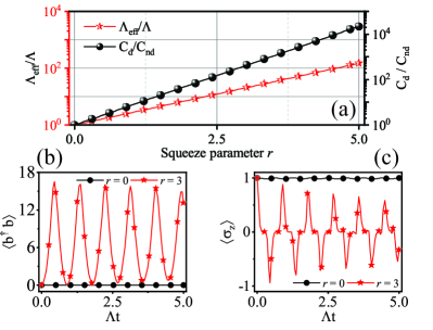
Figure 4: Spin-phonon and phonon-mediated spin-spin coupling. (a) shows $\Lambda_{eff}/\Lambda$ and $C_{d}/C_{nd}$ as a function of the squeezing parameter $r$. The spin-phonon coupling strength appears to be enhanced exponentially. The dynamic processes with ($r=3$) and without ($r=0$) the drive current are shown in (b) and (c). Here the initial state is $|0\rangle|\uparrow\rangle$, where the $|\uparrow\rangle$ represents the excited state $|e\rangle$. The coefficients are $\delta_{m}=10\Lambda$, $\delta_{0}=0$, and $r=0,3$. The dephasing of NV centers and the dissipation of the micromagnet are $\gamma_{NV}=0.01\Lambda$ and $\kappa_{ma}=0.01\Lambda$, respectively.

III.2 Geometric phase

Now we focus on the process of enhancement in phase space. Considering Eq. (16), for the sake of simplicity, we set $\delta_{0}=0$ and move into the Bogoliubov-mode interaction representation. The time evolution operator of the system $U_{RO}(t)=D[\alpha(t)]{\rm exp}[i\Phi(t)\hat{\sigma}_{x}^{2}]$ is obtained via Magnus expansion [93, 94, 95, 96], where $D[\alpha(t)]={\rm exp}{[\alpha(t)\hat{b}^{\dagger}-\alpha^{*}(t)\hat{b}]\hat{\sigma}_{x}}$ is the displacement operator and $\alpha(t)=\Lambda_{eff}/\Delta_{m}(1-e^{i\Delta_{m}t})$ is the coherent displacement of the phonon in phase space. The spin and phonon are decoupled at time $t=2\pi N/\Delta_{m}$ with $N=1,2,3,\cdots$, as shown by the time evolution operator $U_{RO}(t)$, and the phonon returns to its initial state. In Fig. 5(a), the phonon-mode trajectory is shown in phase space. Due to the driving current, the phase space trajectory is magnified and covers a broader area. In addition, the phonon migration direction in phase space is correlated to the spin state, as indicated in equation $D[\alpha(t)]$. Under the original representation, i.e., the interaction representation of phonons, the phase space displacement of phonons is written as $\alpha_{I}(t)=\Lambda/(2\Delta_{m})[({\rm cos}\Delta_{m}t-1)e^{2r}-i{\rm sin}\Delta_{m}t]$  [85, 87].

The geometric phase $\Phi$ is determined only by the enclosed area swept away by phonon trajectories in phase space, as given by

$$\Phi=Im\left[\int_{0}^{t}\alpha^{*}(t^{\prime})\,d\alpha(t^{\prime})\right].$$ (19)

The geometric phase with the driving current at time $t=2\pi/\Delta_{m}$ (phonons orbit once in phase space) is given by $\Phi_{d}=2\pi(\Lambda_{eff}/\Delta_{m})^{2}$. In Fig. 5(b), $\Phi_{d}/\Phi_{nd}\varpropto(e^{r}{\rm cosh}2r)^{2}$ is shown as a function of the squeezing parameter $r$, where $\Phi_{nd}=2\pi(\Lambda/\delta_{m})^{2}$ is the geometric phase sans drive. The geometric phase is roughly exponentially increased. We currently consider acquiring a certain geometric phase $\Phi_{0}$. After that, we can get $t_{d}/t_{nd}\varpropto 1/(e^{r}{\rm cosh}2r)$, where $t_{d}$ and $t_{nd}$ are the time required to acquire $\Phi_{0}$ with and without a drive, respectively. As seen in Fig. 5(b), increasing the squeezing parameter $r$ reduces the time required to acquire a given phase $\Phi_{0}$.

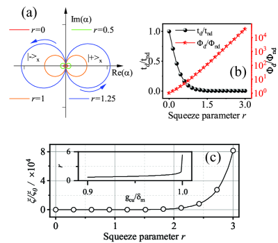
Figure 5: In (a), the phonon trajectory in phase space is depicted, which encloses a larger area as the squeeze parameter increases. (b) geometric phase (in one period) and time (required to acquire a given geometric phase) are depicted as a function of the squeezing parameter $r$. (c) shows that the phonon-mediated spin-spin coupling strength varies with the squeezing parameter $r$. The squeezing parameter $r$ is plotted as a function of the ratio $g_{cu}/\delta_{m}$ in the inset.

III.3 Two NV

We now discuss the interaction of two NV centers with a micromagnet. Two NVs are symmetrically arranged on either side of the micromagnet along the magnetic field direction, coupling to the micromagnet center of mass motion via a strong magnetic field gradient. In the squeezing frame (i.e. with the Bogoliubov transformation [83, 90, 87] $\hat{b}=\hat{a}^{\dagger}{\rm cosh}r-\hat{a}{\rm sinh}r$ and ${\rm tanh}2r=g_{cu}/\delta_{m}$), the Hamiltonian of the hybrid system consisting of the NVs and micromagnet is given by

$$\hat{H}_{RT}=\frac{\delta_{0}}{2}\left(\hat{\sigma}_{z}^{1}+\hat{\sigma}_{z}^{2}\right)+\Delta_{m}\hat{b}^{\dagger}\hat{b}$$ (20)

$$+\Lambda_{eff}\left(\hat{b}+\hat{b}^{\dagger}\right)\left(\hat{\sigma}_{x}^{1}-\hat{\sigma}_{x}^{2}\right).$$

(The complete derivation is given in Appendix D.) With $\delta_{0}=0$, the Hamiltonian can be reduced using the Schrieffer-Wolff transformation [11, 97] $\hat{H}_{RT}^{eff}=e^{S}\hat{H}_{RT}e^{-S}$, where $S=\eta(\hat{b}^{\dagger}-\hat{b})(\hat{\sigma}_{x}^{1}-\hat{\sigma}_{x}^{2})$ and $\eta=\Lambda_{eff}/\Delta_{m}$. It is worth noting that the parameter $\eta$ is usually much smaller than one, indicating that it satisfies the Lamb-Dicke condition $\eta\ll 1$, which is similar to that for trapped ions [98]. The effective Hamiltonian is given by

$$\hat{H}_{RT}^{eff}=\Delta_{m}\hat{b}^{\dagger}\hat{b}\\ -\xi\left(\hat{b}+\hat{b}^{\dagger}\right)\left(\hat{\sigma}_{x}^{1}-\hat{\sigma}_{x}^{2}\right)^{2},$$ (21)

where $\xi=\Lambda_{eff}^{2}/\Delta_{m}$. Retaining only the terms containing $\xi$, we obtain the Ising interaction Hamiltonian

$$\hat{H}_{Ising}=\xi\left(\hat{\sigma}_{x}^{1}-\hat{\sigma}_{x}^{2}\right)^{2},$$ (22)

corresponding to the one-axis twisting interaction [99]. In this scenario, the effective spin-spin interaction of the two NVs is obtained, and the phonon is only virtually excited. Fig. 5(c) shows the coupling strength between two NVs and the insert depicts the squeezing parameter $r$ as a function of $g_{cu}/\delta_{m}$. The ratio of the amplified spin-spin coupling ($\xi=\Lambda_{eff}^{2}/\Delta_{m}$) to the bare coupling ($\xi_{0}=\Lambda^{2}/\delta_{m}$), given by $\xi/\xi_{0}\varpropto(e^{2r}{\rm cosh}2r)^{2}$, exponentially increases. The phonon-mediated spin-spin interaction can be enhanced up to several orders of magnitude stronger than the bare coupling, as the squeezing parameter $r$ increases. It is independent of the specific frame of the phonon since the phonon mode has been adiabatically eliminated. The spin-spin interaction is at the heart of several quantum technologies, such as qubit gates, which are vital for quantum computer implementation. In part IV.2, we will consider a 2-qubit gate with excellent fidelity and faster gate speed.

IV application

IV.1 Preparing Schrödinger cat states

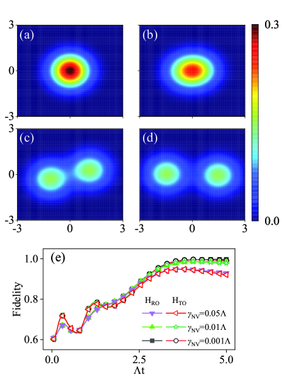
Figure 6: Schrödinger cat states. With $\kappa_{ma}=\gamma_{NV}=0.001\Lambda$, the Winger functions of the phonon mode are displayed in (a), (b), (c), and (d), corresponding to the situations $\Lambda t=0$, $\Lambda t=1.5$, $\Lambda t=3$, and $\Lambda t=4.5$, respectively. (e) The fidelity of the cat state is evaluated with different dephasing rates of the NV center. Furthermore, the dynamic process resulting from $\hat{H}_{RO}$ is identical to that resulting from $\hat{H}_{TO}$. Here, $r(t)=r_{max}\tanh(\Lambda t/2)$ where $r_{max}=1.25$.

The single NV hybrid system can be utilized to prepare a Schrödinger cat state [24, 100], which is a linear superposition of two coherent states. According to the analysis of part III.1, the coupling strength of the NV center and micromagnet has been greatly enhanced, which is critical for preparing a cat state with the spin-mechanical interaction. We assign $\delta_{0}=0$ for the Hamiltonian (14). The Hamiltonian can be diagonalized with the Bogoliubov transformation [83, 90, 87] $\hat{b}=\hat{a}^{\dagger}{\rm cosh}r(t)-\hat{a}{\rm sinh}r(t)$ with ${\rm tanh}2r(t)=g_{cu}(t)/\delta_{m}$, which reads

$$\hat{H}_{TO}=\hat{H}_{RO}+\hat{H}_{Sq}+\hat{H}_{Err},$$ (23)

$$\hat{H}_{RO}=\Delta_{m}\left(t\right)\hat{b}^{\dagger}\hat{b}+\Lambda_{eff}\left(t\right)\left(\hat{b}+\hat{b}^{\dagger}\right)\hat{\sigma}_{x},$$ (24)

$$\hat{H}_{Sq}=\frac{\Lambda e^{-r(t)}}{2}\left(\hat{b}-\hat{b}^{\dagger}\right)\left(\hat{\sigma}^{-}-\hat{\sigma}^{+}\right),$$ (25)

$$\hat{H}_{Err}=-i\frac{\dot{r}(t)}{2}\left(\hat{b}^{\dagger^{2}}-\hat{b}^{2}\right),$$ (26)

where $\Lambda_{eff}\left(t\right)=\Lambda e^{r(t)}/2$ and $\Delta_{m}\left(t\right)=\delta_{m}/{\rm cosh}2r(t)$. $\hat{b}$ ($\hat{b}^{\dagger}$) corresponds to the annihilation (creation) operator of the Bogoliubov mode. The Hamiltonian Eq. (24) is the time-dependent Rabi model, and the undesirable corrections are $\hat{H}_{Sq}$ and $\hat{H}_{Err}$. The Hamiltonian $\hat{H}_{Sq}$ can be ignored since it contains $e^{-r(t)}$, as previously stated. We assume that the pump varies slowly over time to maintain adiabaticity during the dynamical process, such that the correction item $\hat{H}_{Err}$ can be ignored because $\dot{r(t)}\approx 0$. Utilizing Magnus expansion [93, 94, 95, 96], then, the time evolution operator can be written as $U_{RO}(t)=D[\alpha(t)]{\rm exp}[-i\chi(t,0)\hat{b}^{\dagger}\hat{b}]$, where $D[\alpha(t)]={\rm exp}{[\alpha(t)\hat{b}^{\dagger}-\alpha^{*}(t)\hat{b}]\hat{\sigma}_{x}}$ is the displacement operator and $\alpha(t)=-i\Lambda/2\int_{0}^{t}{\rm exp}[r(t^{\prime})-i\chi(t,t^{\prime})]\,dt^{\prime}$ is the coherent displacement of phonons in phase space, with $\chi(t,t^{\prime})=\int_{t^{\prime}}^{t}\Delta_{m}(t^{\prime\prime})\,dt^{\prime\prime}$. The spin-mechanical system is prepared in the initial state $|\Psi_{0}\rangle=|0\rangle|\downarrow\rangle$, with $|\downarrow\rangle$ representing the ground state, and the time evolution operator is then applied to the initial state. Finally, we can obtain an entangled cat state,

$$\Psi_{final}=\frac{|\alpha\left(t\right)\rangle|+\rangle_{x}-|-\alpha\left(t\right)\rangle|-\rangle_{x}}{\sqrt{2}},$$ (27)

where the states $|\pm\alpha(t)\rangle$ are the phonon mode coherent states, and $|\pm\rangle_{x}=(|\uparrow\rangle\pm|\downarrow\rangle)/\sqrt{2}$ are the eigenstates of the operator $\hat{\sigma}_{x}$, with $|\uparrow\rangle$ being the excited state $|e\rangle$. From $t=0$ to $t=t_{f}$, the ideal Rabi Hamiltonian Eq. (24) and the total Hamiltonian Eq. (23) are used to carry out the dynamic simulations of the aforementioned process, respectively. If we assume that the initial state is $|0\rangle|\downarrow\rangle$, the spin dephasing is $\gamma_{NV}$, and the phonon dissipation is $\kappa_{ma}$, the dynamic evolution follows the Lindblad master equation

$$\dot{\hat{\rho}}=-i[\hat{H}_{RO}/\hat{H}_{TO},\hat{\rho}]+\gamma_{NV}D\left(\hat{\sigma}_{z}\right)\hat{\rho}+\kappa_{ma}D(\hat{b})\hat{\rho},$$ (28)

where $D(\hat{O})\hat{\rho}=\hat{O}\hat{\rho}\hat{O}^{\dagger}-\{\hat{O}^{\dagger}\hat{O},\hat{\rho}\}/2$ is the Lindblad operator. Figs. 6(a), (b), (c), and (d) depict the evolution of the phonon-mode Winger function over time using the Hamiltonian $\hat{H}_{RO}$. At the initial time $t=0$, the squeezed parameter $r(0)=0$, indicating that the current drive is zero, and the system is prepared in the initial state $|0\rangle|\downarrow\rangle$ [84, 17]. The current drive is loaded adiabatically over time and then, the transformed-$b$-mode evolves into a well-separated Schrödinger cat state in phase space. In addition, the fidelity of the cat state is depicted in Fig. 6(e) (with the Hamiltonian $\hat{H}_{RO}$), achieving $99.7\%$ when $\gamma_{NV}=0.001\Lambda$, $98.3\%$ when $\gamma_{NV}=0.01\Lambda$, and $92.8\%$ when $\gamma_{NV}=0.05\Lambda$. It is worth noticing that the evolution predicted by $\hat{H}_{RO}$ (solid lines with open symbols) matches that predicted by $\hat{H}_{TO}$ (the solid line with close symbols). It suggests that the unwanted corrections produced by $\hat{H}_{Sq}$ and $\hat{H}_{Err}$ can be ignored.

IV.2 Two-qubit gate

Quantum logic gates [101, 102, 94, 103, 104] are the core of quantum computation. Geometric quantum computing refers to the quantum computation associated with the pure geometric phase [105, 106]. Based on the different methods of obtaining geometric phase, the geometric phase gate can be divided into two categories: (i) the conventional geometric phase gate, which acquires the pure geometric phase with adiabatic evolution of qubits; and (ii) the unconventional geometric phase gate, which acquires the pure geometric phase with the evolution of the bose mode along a close trajectory in the phase space [105, 107]. Conventional geometric phase gates have been studied with many platforms [106, 108, 109]. The two-NV proposal, as discussed in part III.3, can be utilized to build an unconventional geometric phase 2-qubit gate with high fidelity and faster gate speed. The hybrid system containing two NVs is described by the Hamiltonian (20). As previously discussed, we set $\delta_{0}=0$, and $\hat{b}$ ($\hat{b}^{\dagger}$) corresponds to the Bogoliubov mode annihilation (creation) operator. Moving in the Bogoliubov-mode interaction frame, we can get

$$\hat{H}_{RT}^{I}=\Lambda_{eff}\left(\hat{b}e^{-i\Delta_{m}t}+\hat{b}^{\dagger}e^{i\Delta_{m}t}\right)\left(\hat{\sigma}_{x}^{1}-\hat{\sigma}_{x}^{2}\right).$$ (29)

Then, utilizing the Magnus expansion [93, 94, 95, 96], the time evolution operator is given by

$$U_{RT}(t)=D[\alpha(t)]E_{ij}[\beta(t)],$$ (30)

where $D[\alpha(t)]={\rm exp}{[\alpha(t)\hat{b}^{\dagger}-\alpha^{*}(t)\hat{b}]\hat{\sigma}_{x}}$ denotes the displacement operator, and $\alpha(t)=\Lambda_{eff}/\Delta_{m}(1-e^{i\Delta_{m}t})$ is the coherent displacement of phonons in phase space. The second item describing spin-spin interaction is given by

$$E_{ij}[\beta(t)]={\rm exp}\left(\sum_{i,j}^{2}\beta\eta_{ij}\hat{\sigma}_{x}^{i}\hat{\sigma}_{x}^{j}\right),$$ (31)

where

$$\eta_{ij}=\left\{\begin{array}[]{c}1,i=j\\ -1,i\neq j\end{array}\right..$$ (32)

The phonon mode returning to its initial state, a gate operation is completed. As a result, the gate time is determined by $\tau=2\pi/\Delta_{m}$, at which point the time evolution operator can be represented as

$$U_{RT}(\tau)={\exp}\left(-i2\pi\frac{\Lambda_{eff}^{2}}{\Delta_{m}^{2}}\sum_{i,j}^{2}\eta_{ij}\hat{\sigma}_{x}^{i}\hat{\sigma}_{x}^{j}\right).$$ (33)

Adjusting the ratio between $\Lambda_{eff}$ and $\Delta_{m}$, qubit gates corresponding to different phases can be constructed, such as the $\pi/2$-2-qubit gate described by $U_{RT}(\tau)={\rm exp}(-i\frac{\pi}{8}\sum_{i,j}^{2}\eta_{ij}\hat{\sigma}_{x}^{i}\hat{\sigma}_{x}^{j})$. Supposing that the initial state is the eigenstate of $\hat{\sigma}_{x}$, then, at time $\tau$, the final state is

$$\begin{array}[]{c}|+\rangle_{x}|+\rangle_{x}\rightarrow|+\rangle_{x}|+\rangle_{x},\\ |-\rangle_{x}|-\rangle_{x}\rightarrow|-\rangle_{x}|-\rangle_{x},\\ |+\rangle_{x}|-\rangle_{x}\rightarrow e^{-i\pi/2}|+\rangle_{x}|-\rangle_{x},\\ |-\rangle_{x}|+\rangle_{x}\rightarrow e^{-i\pi/2}|-\rangle_{x}|+\rangle_{x}.\end{array}$$ (34)

The 2-qubit gate only adds phase to $|+\rangle_{x}|-\rangle_{x}$ and $|-\rangle_{x}|+\rangle_{x}$, not $|+\rangle_{x}|+\rangle_{x}$ and $|-\rangle_{x}|-\rangle_{x}$, because the time evolution operator at time $\tau$ is $\hat{I}$ when the initial state is the latter. Furthermore, the 2-qubit gate is universal, as demonstrated in the literature [110].

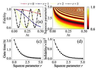
Figure 7: 2-qubit gate. The dynamic process of the $2$-qubit gate is presented in (a), (b) with the varying squeezing parameter $r$. When the phonon mode evolves back to the original state, a gate operation is accomplished. In (c) and (d), gate time and the infidelity of the $2$-qubit gate are shown as a function of the squeezing parameter $r$. The larger the squeezing parameter $r$, the shorter the gate-time and the smaller the gate infidelity. Here, the parameters are $\kappa_{ma}=\gamma_{NV}^{1}=\gamma_{NV}^{2}=0.01\Lambda$, $\delta_{0}=0$, $\Delta_{m}=4\Lambda_{eff}$ and the initial state is $|+\rangle_{x}|-\rangle_{x}$.

Utilizing Eq. (20) for numerical simulations with the dissipation of the phonon mode $\kappa_{ma}$ and the dephasing of NVs $\gamma_{NV}^{1}$ and $\gamma_{NV}^{2}$, the dynamic process can be described by the Lindblad master equation

$$\dot{\hat{\rho}}=-i[\hat{H}_{RT},\hat{\rho}]+\kappa_{ma}D(\hat{b})\hat{\rho}$$ (35)

$$+\gamma_{NV}^{1}D(\hat{\sigma}_{z}^{1})\hat{\rho}+\gamma_{NV}^{2}D(\hat{\sigma}_{z}^{2})\hat{\rho},$$

where $D(\hat{O})\hat{\rho}=\hat{O}\hat{\rho}\hat{O}^{\dagger}-\{\hat{O}^{\dagger}\hat{O},\hat{\rho}\}/2$. As depicted in Figs. 7(a)(b), when the fidelity of the phonon mode reaches its maximum value, a gate operation is finished. It reveals that 2-qubit gate time decreases as the squeezing parameter $r$ increases. Furthermore, Fig. 7(c) indicates that with the squeezing parameter $r$ increasing, the gate time decreases dramatically. The 2-qubit-gate infidelity, arising from the dephasing of the spins is also affected by the squeezing parameter $r$ shown in Fig. 7(d). It indicates that a 2-qubit gate with higher fidelity and shorter gate time can be achieved, with the fidelity being more than $99.9\%$ when the squeezing parameter $r=3$.

V Experimental feasibility

To verify the experimental feasibility of the scheme proposed in this paper, we consider the scheme based on the experimental parameters given in ref. [51], which include the radius $a=0.25\rm~{}{\mu}m$, cooling height $h_{cool}=3a$, equilibrium position $h_{eq}=3a$, cooling angle $\phi_{cool}=\pi/2$ and $\theta_{cool}=0$, equilibrium angle $\phi=\pi/2$ and $\theta=0$, the density of micromagnet $\rho=7430\rm~{}{kg/m^{3}}$, and residual induction $B_{r}=750\rm~{}{mT}$. In this case, the coupling strength between the NV center and the micromagnet is $2.9$ kHz, which is consistent with ref. [51]. A driving current is applied to the hybrid system, with the position $h_{cu}=2h_{eq}$ and amplitude $I_{0}=10\rm~{}{mA}$. The magnetic field induced by the current in the position of the NV center is $2\rm~{}{mT}$. If the static transverse magnetic field is $10$ times larger than the magnetic field induced by the driving current, the influence of the current on the NV center can be neglected.

Fig. 8(a) shows the coupling strength between the driving current and the micromagnet as a function of the distance between them $d_{CU-MA}$. As the distance between them grows, it decreases, reaching $10$ MHz when $d_{CU-MA}=0.3\rm~{}{\mu}m$. The coupling strength between the NV center and the micromagnet as a function of the distance between them $d_{NV-MA}$ and the squeezing parameter $r$ is depicted in Fig. 8(b). This shows that the coupling strength can be amplified when decreasing the distance and increasing the squeezing parameter $r$, reaching $1.2$ MHz if $d_{NV-MA}=0.3\rm~{}{\mu}m$ and the squeezing parameter $r=5$, indicating that it can reach the strong and even ultra-strong regime. To summarize, we can choose appropriate parameters based on the actual experimental conditions. In addition, the proposal is simple to implement under current experimental circumstances.

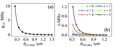
Figure 8: (a) the coupling strength between the driving current and the micromagnet varies with the distance between them. (b) indicates that the coupling strength of the NV and micromagnet grows as the distance between them decreases and the squeezing parameter $r$ increases.

VI Conclusion

Utilizing NV centers and a levitated micromagnet, we propose a hybrid quantum spin-mechanical system. A time-dependent driving current is applied to the hybrid system, which offers the critical nonlinear resource for the enhancement of the coupling strength. As a result, the spin-phonon and phonon-medicated spin-spin coupling strengths can be enhanced exponentially. The system can be utilized to construct an unconventional 2-qubit geometric phase gate with high fidelity and shorter gate time, as well as to prepare Schrödinger cat states with high fidelity. Furthermore, the Ground-state cooling approach, which requires the ultrastrong interaction between qubits and oscillators described by ref. [15], could be more simply implemented with this proposal. In addition, because the trapped frequency is related to the levitated height and the radius of the micromagnet, a wide frequency range can be easily obtained. Our proposal can also be extended to other solid-state spin systems, such as the silicon-vacancy center, germanium-vacancy center, and tin-vacancy center in diamond [37, 17, 40], allowing for more quantum information processing applications based on quantum levitodynamics.

Appendix A Levitation of the micromagnet

In our scheme, we use a Type-II superconductor to levitate a micromagnet. The principle of levitation can be analytically analyzed by the frozen dipole model [89, 51]. As shown in Fig. 1(c), the position vector of frozen and image dipoles are $\bm{R_{f}}=(-h_{cool},0,0)$ and $\bm{R_{\rm i}}=(-x,y,z)$, respectively. The orientation corresponds to $\bm{\mu_{f}}=\mu_{m}({\rm sin}\theta_{cool},0,-{\rm cos}\theta_{cool})$ and $\bm{\mu_{\rm i}}=\mu_{m}(-{\rm cos}\phi{\rm sin}\theta,{\rm sin}\phi{\rm sin}\theta,{\rm cos}\theta)$, respectively. The magnetic field produced by a dipole $\bm{\mu}$ at a position $\bm{r}$ is given by

$$\bm{B}=\frac{\mu_{0}}{4\pi}\left(\frac{3\bm{r}\left(\bm{\mu\cdot r}\right)}{r^{5}}-\frac{\bm{\mu}}{r^{3}}\right).$$ (36)

The effective magnetic field $\bm{B_{eff}}$ is composed of the magnetic field generated by the frozen dipole and image dipole, which is written as $\bm{B_{eff}}=\bm{B_{f}}+\bm{B_{i}}/2$  [51]. In this case, the total potential energy of the levitated micromagnet is given by

$$U=-\bm{\mu\cdot B_{eff}}+mgx,$$ (37)

where $\bm{\mu}=\mu_{m}({\rm cos}\phi{\rm sin}\theta,{\rm sin}\phi{\rm sin}\theta,{\rm cos}\theta)$, $g=9.8m/s^{2}$, and $m$ is the mass of the micromagnet. For convenience, the potential energy in dimensionless form with $x_{s}=x/a$, $y_{s}=y/a$, and $z_{s}=z/a$ can be represented as

$$U=U_{s}\left(\alpha_{s}x_{s}+g_{u}\right),$$ (38)

where $\alpha_{s}=a/\alpha_{crit}$, $U_{s}=mg\alpha_{crit}$, $\alpha_{crit}=B_{r}^{2}/(16g\rho\mu_{0})$, and

$$g_{u}=\frac{1+\left({\rm cos}\phi{\rm sin}\theta\right)^{2}}{3x^{3}}$$

$$-\frac{16}{3}\frac{g_{c}{\rm cos}\theta+g_{s}{\rm sin}\theta}{\left[\left(x+h_{cool}\right)^{2}+y^{2}+z^{2}\right]^{5/2}},$$ (39a)

$$g_{c}=\left[\left(x+h_{cool}\right)^{2}+y^{2}-2z^{2}\right]{\rm cos}\theta_{cool}$$

$$+3z\left(x+h_{cool}\right){\rm sin}\theta_{cool},$$ (39b)

$$g_{s}=\left[-3z\left(x+h_{cool}\right){\rm cos}\phi-3zy{\rm sin}\phi\right]{\rm cos}\theta_{cool}$$

$$+\Big{\{}\left[2\left(x+h_{cool}\right)^{2}-y^{2}-z^{2}\right]{\rm cos}\phi$$

$$+3y\left(x+h_{cool}\right){\rm sin}\phi\Big{\}}{\rm sin}\theta_{cool}.$$ (39c)

We now consider solely the potential energy along the $z$-direction, denoted by

$$\mathrm{U}=U_{s}\left\{\frac{16}{3}\frac{2z^{2}-\left(h_{eq}+h_{cool}\right)^{2}}{\left[\left(h_{eq}+h_{cool}\right)^{2}+z^{2}\right]^{5/2}}+\frac{1}{3h_{eq}^{3}}+\alpha_{s}h_{eq}\right\},$$ (40)

where $h_{eq}$ and $h_{cool}$ correspond to the equilibrium position and the cooling height, respectively. According to the analysis in part II.2, we assign $\phi=\phi_{cool}=\pi/2$ and $\theta=\theta_{cool}=0$, which means that the direction of levitation represented by $\theta$ and $\phi$ is the same as the initial orientation $\theta_{cool}$ and $\phi_{cool}$. This indicates that the rotation of the micromagnet is neglected. By expanding at the equilibrium position and removing the constant and high order components, the potential energy can be written as simple harmonic potential

$$U=\frac{1}{2}k_{ma}z^{2},$$ (41)

where

$$k_{ma}=\frac{\mu_{0}\mu_{m}^{2}}{4\pi}\frac{3}{\left(h_{eq}+h_{cool}\right)^{5}}.$$ (42)

The motion of the levitated micromagnet along the $z$-direction can be regarded as a simple harmonic motion, as represented by

$$\hat{H}_{magnet}=\frac{\hat{p}^{2}}{2m}+\frac{1}{2}k_{ma}\hat{z}^{2},$$ (43)

where $\hat{p}_{z}$ and $\hat{z}$ are momentum and position operators, respectively. By quantizing the Hamiltonian with $\hat{p}_{z}=-i\sqrt{m\omega_{ma}/2}(\hat{a}-\hat{a}^{\dagger})$, $\hat{z}=z_{0}(\hat{a}+\hat{a}^{\dagger})$, and $z_{0}=\sqrt{1/(2m\omega_{ma})}$, we can obtain

$$\hat{H}_{magnet}=\omega_{ma}\hat{a}^{\dagger}\hat{a},$$ (44)

where $\omega_{ma}=\sqrt{k_{ma}/m}$ represents the trapping frequency associated with the cooling conditions, and $\hat{a}$ ($\hat{a}^{\dagger}$) represents the annihilation (creation) operator.

Appendix B Interaction between NV and micromagnet

The NV center is coupled to the levitated micromagnet via a strong magnetic field gradient. Firstly, we investigate how one NV center interacts with a micromagnet. In our proposal, the micromagnet is described as a dipole with $\bm{\mu}=\mu_{m}({\rm cos}\phi{\rm sin}\theta,{\rm sin}\phi{\rm sin}\theta,{\rm cos}\theta)$ at position $(x,y,z)$. At position $(h_{eq},0,d)$ of the NV center, the magnetic field induced by the micromagnet along the $z$-direction is given by

$$\bm{B_{ma}}=\frac{\mu_{0}\mu_{m}}{2\pi\left(d-z\right)^{3}}\bm{\hat{e}_{z}}.$$ (45)

By expanding at the equilibrium position, removing the constant and high order terms, the magnetic field can be written as

$$\bm{B_{ma}}=\frac{3\mu_{0}\mu_{m}}{4\pi d^{4}}z\bm{\hat{e}_{z}}.$$ (46)

Therefore, the interaction Hamiltonian is given by

$$\hat{H}_{int}=\gamma_{e}\frac{3\mu_{0}\mu_{m}}{4\pi d^{4}}\hat{z}\hat{S}_{z}.$$ (47)

Quantizing the Hamiltonian, we can obtain

$$\hat{H}_{int}=\lambda\left(\hat{a}+\hat{a}^{\dagger}\right)\hat{S}_{z},$$ (48)

where $\lambda=\gamma_{e}B_{r}a^{3}z_{0}/d^{4}$ is the coupling strength.

What is more intriguing is that two NVs are symmetrically placed at positions $(h_{eq},0,d)$ and $(h_{eq},0,-d)$ on either side of the micromagnet along the direction of magnetization. Along the $z$-axis, the magnetic field produced by the micromagnet is given by

$$\bm{B_{1}}=\frac{\mu_{0}\mu_{m}}{2\pi\left(d-z\right)^{3}}\bm{\hat{e}_{z}},$$ (49a)

$$\bm{B_{2}}=\frac{\mu_{0}\mu_{m}}{2\pi\left(d+z\right)^{3}}\bm{\hat{e}_{z}}.$$ (49b)

After expanding at the equilibrium position, omitting constant items and high order components, the magnetic field can be represented as

$$\bm{B_{1}}=\frac{3\mu_{0}\mu_{m}}{4\pi d^{4}}z\bm{\hat{e}_{z}},$$ (50a)

$$\bm{B_{2}}=-\frac{3\mu_{0}\mu_{m}}{4\pi d^{4}}z\bm{\hat{e}_{z}}.$$ (50b)

In the same way as the one-NV process, we can get the interaction Hamiltonian of two NV centers, which reads

$$\hat{H}_{int}=\lambda\left(\hat{a}+\hat{a}^{\dagger}\right)\left(\hat{S}_{z}^{1}-\hat{S}_{z}^{2}\right),$$ (51)

where $\lambda=\gamma_{e}B_{r}a^{3}z_{0}/d^{4}$ is the coupling strength.

Appendix C The Hamiltonian of drive current

Current pumping $I_{cu}(t)=I_{0}{\rm cos}2\omega_{cu}t$ is added to the hybrid system to enhance coupling strength. The position of origin current and image current in the $zx$-plane are $\bm{R_{or}}=(h_{cu},0,0)$ and $\bm{R_{im}}=(-h_{cu},0,0)$, respectively. When just the magnetic field in the $z$-direction near the equilibrium position is considered, the total magnetic field created by the origin and image current is given by

$$\bm{B_{cu}}=\bm{B_{or}}+\bm{B_{im}}=\frac{\mu_{0}I}{2\pi}\left(\frac{1}{r_{or}}+\frac{1}{r_{im}}\right)\bm{\hat{e}_{z}}.$$ (52)

Then the potential energy of the micromagnet in the magnetic field generated by the current can be written as

$$U_{cu}=-\bm{\mu\cdot B_{cu}},$$ (53a)

$$U_{cu}=-\frac{\mu_{0}\mu_{m}I}{2\pi}\left[\frac{1}{\sqrt{\left(h_{eq}-h_{cu}\right)^{2}+z^{2}}}\right]$$

$$-\frac{\mu_{0}\mu_{m}I}{2\pi}\left[\frac{1}{\sqrt{\left(h_{eq}+h_{cu}\right)^{2}+z^{2}}}\right].$$ (53b)

By expanding at the equilibrium position, dropping constant items and high order terms, the magnetic field can be represented as

$$U_{cu}=-\frac{1}{2}k_{cu}\hat{z}^{2}{\rm cos}2\omega_{cu}t,$$ (54)

where

$$k_{cu}=\frac{\mu_{0}\mu_{m}I_{0}}{2\pi}\left[\frac{1}{\left(h_{cu}-h_{eq}\right)^{3}}+\frac{1}{\left(h_{cu}+h_{eq}\right)^{3}}\right].$$ (55)

Quantizing the potential energy, the Hamiltonian is given by

$$\hat{H}_{cu}=-g_{cu}\left(\hat{a}+\hat{a}^{\dagger}\right)^{2}{\rm cos}2\omega_{cu}t,$$ (56)

where $g_{cu}=k_{cu}z_{0}^{2}/2$ is the coupling strength between the drive current and the micromagnet.

Appendix D The total Hamiltonian of the hybrid system (two NVs)

This section will derive the Hamiltonian, which describes the interaction between two NVs and the micromagnet. Two NV centers are symmetrically arranged on either side of the micromagnet, coupling to the center of mass motion of the micromagnet through a strong magnetic field gradient produced by the micromagnet. The Hamiltonian of the hybrid system is given by

$$\hat{H}_{TT}=\frac{\omega_{0}}{2}\left(\hat{\sigma}_{z}^{1}+\hat{\sigma}_{z}^{2}\right)+\omega_{ma}\hat{a}^{\dagger}\hat{a}$$ (57)

$$+\Lambda\left(\hat{a}+\hat{a}^{\dagger}\right)\left(\hat{\sigma}_{x}^{1}-\hat{\sigma}_{x}^{2}\right)-g_{cu}\left(\hat{a}+\hat{a}^{\dagger}\right)^{2}{\rm cos}2\omega_{cu}t.$$

Moving in the rotation frame, the Hamiltonian can be simplified as

$$\hat{H}_{TT}=\frac{\omega_{0}}{2}\left(\hat{\sigma}_{z}^{1}+\hat{\sigma}_{z}^{2}\right)+\omega_{ma}\hat{a}^{\dagger}\hat{a}$$ (58)

$$+\Lambda\left[\hat{a}\left(\hat{\sigma}_{1}^{+}-\hat{\sigma}_{2}^{+}\right)+\hat{a}^{\dagger}\left(\hat{\sigma}_{1}^{-}-\hat{\sigma}_{2}^{-}\right)\right]-\frac{g_{cu}}{2}\left(\hat{a}^{2}+\hat{a}^{\dagger^{2}}\right).$$

Utilizing the Bogoliubov transformation [83, 90, 87] $\hat{b}=\hat{a}^{\dagger}{\rm cosh}r-\hat{a}{\rm sinh}r$ and ${\rm tanh}2r=g_{cu}/\delta_{m}$, the total Hamiltonian can be diagonalized and represented as

$$H_{RT}=\frac{\delta_{0}}{2}\left(\hat{\sigma}_{z}^{1}+\hat{\sigma}_{z}^{2}\right)+\Delta_{m}\hat{b}^{\dagger}\hat{b}$$ (59)

$$+\Lambda_{eff}\left(\hat{b}+\hat{b}^{\dagger}\right)\left(\hat{\sigma}_{x}^{1}-\hat{\sigma}_{x}^{2}\right).$$

Without loss of generality, we assume the $\delta_{0}=0$, such that the Hamiltonian can be simplified by a Schrieffer-Wolff transformation [11, 97] $\hat{H}_{RT}^{eff}=e^{S}\hat{H}_{RT}e^{-S}$, where $S=\eta(\hat{b}^{\dagger}-\hat{b})(\hat{\sigma}_{x}^{1}-\hat{\sigma}_{x}^{2})$ with $\eta=\Lambda_{eff}/\Delta_{m}$ and the Lamb-Dicke condition $\eta\ll 1$. The effective Hamiltonian is given by

$$\hat{H}_{RT}^{eff}=\Delta_{m}\hat{b}^{\dagger}\hat{b}-\xi\left(\hat{b}+\hat{b}^{\dagger}\right)\left(\hat{\sigma}_{x}^{1}-\hat{\sigma}_{x}^{2}\right)^{2},$$ (60)

where $\xi=\Lambda_{eff}^{2}/\Delta_{m}$. Retaining only the terms containing $\xi$, we obtain the Ising interaction Hamiltonian

$$\hat{H}_{Ising}=\xi\left(\hat{\sigma}_{x}^{1}-\hat{\sigma}_{x}^{2}\right)^{2},$$ (61)

which corresponds to the one-axis twisting interaction.

References

- Xiang et al. [2013] Z.-L. Xiang, S. Ashhab, J. Q. You, and F. Nori, Hybrid quantum circuits: Superconducting circuits interacting with other quantum systems, Rev. Mod. Phys. 85, 623 (2013).
- Clerk et al. [2020] A. A. Clerk, K. W. Lehnert, P. Bertet, J. R. Petta, and Y. Nakamura, Hybrid quantum systems with circuit quantum electrodynamics, Nat. Phys. 16, 257 (2020).
- Wallquist et al. [2009] M. Wallquist, K. Hammerer, P. Rabl, M. Lukin, and P. Zoller, Hybrid quantum devices and quantum engineering, Phys. Scr. T137, 014001 (2009).
- Walther et al. [2006] H. Walther, B. T. H. Varcoe, B.-G. Englert, and T. Becker, Cavity quantum electrodynamics, Rep. Prog. Phys. 69, 1325 (2006).
- Blais et al. [2021] A. Blais, A. L. Grimsmo, S. M. Girvin, and A. Wallraff, Circuit quantum electrodynamics, Rev. Mod. Phys. 93, 025005 (2021).
- Huillery et al. [2020] P. Huillery, T. Delord, L. Nicolas, M. Van Den Bossche, M. Perdriat, and G. Hétet, Spin mechanics with levitating ferromagnetic particles, Phys. Rev. B 101, 134415 (2020).
- Dong et al. [2021] X.-L. Dong, P.-B. Li, T. Liu, and F. Nori, Unconventional quantum sound-matter interactions in spin-optomechanical-crystal hybrid systems, Phys. Rev. Lett. 126, 203601 (2021).
- Arcizet et al. [2011] O. Arcizet, V. Jacques, A. Siria, P. Poncharal, P. Vincent, and S. Seidelin, A single nitrogen-vacancy defect coupled to a nanomechanical oscillator, Nat. Phys. 7, 879 (2011).
- Hong et al. [2012] S. Hong, M. S. Grinolds, P. Maletinsky, R. L. Walsworth, M. D. Lukin, and A. Yacoby, Coherent, mechanical control of a single electronic spin, Nano. Lett. 12, 3920 (2012).
- Kolkowitz et al. [2012] S. Kolkowitz, A. C. B. Jayich, Q. P. Unterreithmeier, S. D. Bennett, P. Rabl, J. G. E. Harris, and M. D. Lukin, Coherent sensing of a mechanical resonator with a single-spin qubit, Science 335, 1603 (2012).
- Wilson-Rae et al. [2004] I. Wilson-Rae, P. Zoller, and A. Imamoḡlu, Laser cooling of a nanomechanical resonator mode to its quantum ground state, Phys. Rev. Lett. 92, 075507 (2004).
- Li et al. [2015] P.-B. Li, Y.-C. Liu, S.-Y. Gao, Z.-L. Xiang, P. Rabl, Y.-F. Xiao, and F.-L. Li, Hybrid quantum device based on centers in diamond nanomechanical resonators plus superconducting waveguide cavities, Phys. Rev. Applied 4, 044003 (2015).
- Bennett et al. [2013] S. D. Bennett, N. Y. Yao, J. Otterbach, P. Zoller, P. Rabl, and M. D. Lukin, Phonon-induced spin-spin interactions in diamond nanostructures: Application to spin squeezing, Phys. Rev. Lett. 110, 156402 (2013).
- Kepesidis et al. [2013] K. V. Kepesidis, S. D. Bennett, S. Portolan, M. D. Lukin, and P. Rabl, Phonon cooling and lasing with nitrogen-vacancy centers in diamond, Phys. Rev. B 88, 064105 (2013).
- Streltsov et al. [2021] K. Streltsov, J. S. Pedernales, and M. B. Plenio, Ground-state cooling of levitated magnets in low-frequency traps, Phys. Rev. Lett. 126, 193602 (2021).
- Rabl et al. [2009] P. Rabl, P. Cappellaro, M. V. G. Dutt, L. Jiang, J. R. Maze, and M. D. Lukin, Strong magnetic coupling between an electronic spin qubit and a mechanical resonator, Phys. Rev. B 79, 041302 (2009).
- Li et al. [2020] P.-B. Li, Y. Zhou, W.-B. Gao, and F. Nori, Enhancing spin-phonon and spin-spin interactions using linear resources in a hybrid quantum system, Phys. Rev. Lett. 125, 153602 (2020).
- Xu et al. [2009] Z. Y. Xu, Y. M. Hu, W. L. Yang, M. Feng, and J. F. Du, Deterministically entangling distant nitrogen-vacancy centers by a nanomechanical cantilever, Phys. Rev. A 80, 022335 (2009).
- Chotorlishvili et al. [2013] L. Chotorlishvili, D. Sander, A. Sukhov, V. Dugaev, V. R. Vieira, A. Komnik, and J. Berakdar, Entanglement between nitrogen vacancy spins in diamond controlled by a nanomechanical resonator, Phys. Rev. B 88, 085201 (2013).
- Zhou et al. [2010] L.-g. Zhou, L. F. Wei, M. Gao, and X.-b. Wang, Strong coupling between two distant electronic spins via a nanomechanical resonator, Phys. Rev. A 81, 042323 (2010).
- Rabl et al. [2010] P. Rabl, S. J. Kolkowitz, F. H. L. Koppens, J. G. E. Harris, P. Zoller, and M. D. Lukin, A quantum spin transducer based on nanoelectromechanical resonator arrays, Nat. Phys. 6, 602 (2010).
- Ovartchaiyapong et al. [2014] P. Ovartchaiyapong, K. W. Lee, B. A. Myers, and A. C. B. Jayich, Dynamic strain-mediated coupling of a single diamond spin to a mechanical resonator, Nat. Commun. 5, 4429 (2014).
- Teissier et al. [2014] J. Teissier, A. Barfuss, P. Appel, E. Neu, and P. Maletinsky, Strain coupling of a nitrogen-vacancy center spin to a diamond mechanical oscillator, Phys. Rev. Lett. 113, 020503 (2014).
- Asjad and Vitali [2014] M. Asjad and D. Vitali, Reservoir engineering of a mechanical resonator: generating a macroscopic superposition state and monitoring its decoherence, J. Phys. B: At. Mol. Opt. Phys. 47, 045502 (2014).
- Sánchez Muñoz et al. [2018] C. Sánchez Muñoz, A. Lara, J. Puebla, and F. Nori, Hybrid systems for the generation of nonclassical mechanical states via quadratic interactions, Phys. Rev. Lett. 121, 123604 (2018).
- MacQuarrie et al. [2013] E. R. MacQuarrie, T. A. Gosavi, N. R. Jungwirth, S. A. Bhave, and G. D. Fuchs, Mechanical spin control of nitrogen-vacancy centers in diamond, Phys. Rev. Lett. 111, 227602 (2013).
- Pigeau et al. [2015] B. Pigeau, S. Rohr, L. Mercier de Lépinay, A. Gloppe, V. Jacques, and O. Arcizet, Observation of a phononic mollow triplet in a multimode hybrid spin-nanomechanical system, Nat. Commun. 6, 8603 (2015).
- Carter et al. [2018] S. G. Carter, A. S. Bracker, G. W. Bryant, M. Kim, C. S. Kim, M. K. Zalalutdinov, M. K. Yakes, C. Czarnocki, J. Casara, M. Scheibner, and D. Gammon, Spin-mechanical coupling of an inas quantum dot embedded in a mechanical resonator, Phys. Rev. Lett. 121, 246801 (2018).
- Li et al. [2016a] P.-B. Li, Z.-L. Xiang, P. Rabl, and F. Nori, Hybrid quantum device with nitrogen-vacancy centers in diamond coupled to carbon nanotubes, Phys. Rev. Lett. 117, 015502 (2016a).
- Lemmer et al. [2013] A. Lemmer, A. Bermudez, and M. B. Plenio, Driven geometric phase gates with trapped ions, New J. Phys. 15, 083001 (2013).
- Porras and Cirac [2004] D. Porras and J. I. Cirac, Effective quantum spin systems with trapped ions, Phys. Rev. Lett. 92, 207901 (2004).
- Britton et al. [2012] J. W. Britton, B. C. Sawyer, A. C. Keith, C. C. J. Wang, J. K. Freericks, H. Uys, M. J. Biercuk, and J. J. Bollinger, Engineered two-dimensional ising interactions in a trapped-ion quantum simulator with hundreds of spins, Nature 484, 489 (2012).
- Martinetz et al. [2020] L. Martinetz, K. Hornberger, J. Millen, M. S. Kim, and B. A. Stickler, Quantum electromechanics with levitated nanoparticles, npj Quantum Inf. 6, 101 (2020).
- Delord et al. [2017] T. Delord, L. Nicolas, Y. Chassagneux, and G. Hétet, Strong coupling between a single nitrogen-vacancy spin and the rotational mode of diamonds levitating in an ion trap, Phys. Rev. A 96, 063810 (2017).
- Barry et al. [2020] J. F. Barry, J. M. Schloss, E. Bauch, M. J. Turner, C. A. Hart, L. M. Pham, and R. L. Walsworth, Sensitivity optimization for nv-diamond magnetometry, Rev. Mod. Phys. 92, 015004 (2020).
- Doherty et al. [2013] M. W. Doherty, N. B. Manson, P. Delaney, F. Jelezko, J. Wrachtrup, and L. C. Hollenberg, The nitrogen-vacancy colour centre in diamond, Phys. Rep. 528, 1 (2013).
- Bradac et al. [2019] C. Bradac, W. Gao, J. Forneris, M. E. Trusheim, and I. Aharonovich, Quantum nanophotonics with group iv defects in diamond, Nat. Commun. 10, 5625 (2019).
- Meesala et al. [2018] S. Meesala, Y.-I. Sohn, B. Pingault, L. Shao, H. A. Atikian, J. Holzgrafe, M. Gündoğan, C. Stavrakas, A. Sipahigil, C. Chia, R. Evans, M. J. Burek, M. Zhang, L. Wu, J. L. Pacheco, J. Abraham, E. Bielejec, M. D. Lukin, M. Atatüre, and M. Lončar, Strain engineering of the silicon-vacancy center in diamond, Phys. Rev. B 97, 205444 (2018).
- Lemonde et al. [2018] M.-A. Lemonde, S. Meesala, A. Sipahigil, M. J. A. Schuetz, M. D. Lukin, M. Loncar, and P. Rabl, Phonon networks with silicon-vacancy centers in diamond waveguides, Phys. Rev. Lett. 120, 213603 (2018).
- Hepp et al. [2014] C. Hepp, T. Müller, V. Waselowski, J. N. Becker, B. Pingault, H. Sternschulte, D. Steinmüller-Nethl, A. Gali, J. R. Maze, M. Atatüre, and C. Becher, Electronic structure of the silicon vacancy color center in diamond, Phys. Rev. Lett. 112, 036405 (2014).
- Chen et al. [2021] J.-Q. Chen, Y.-F. Qiao, X.-L. Dong, X.-L. Hei, and P.-B. Li, Dissipation-assisted preparation of steady spin-squeezed states of siv centers, Phys. Rev. A 103, 013709 (2021).
- Prat-Camps et al. [2017] J. Prat-Camps, C. Teo, C. C. Rusconi, W. Wieczorek, and O. Romero-Isart, Ultrasensitive inertial and force sensors with diamagnetically levitated magnets, Phys. Rev. Applied 8, 034002 (2017).
- Timberlake et al. [2019] C. Timberlake, G. Gasbarri, A. Vinante, A. Setter, and H. Ulbricht, Acceleration sensing with magnetically levitated oscillators above a superconductor, Appl. Phys. Lett. 115, 224101 (2019).
- Vinante et al. [2020] A. Vinante, P. Falferi, G. Gasbarri, A. Setter, C. Timberlake, and H. Ulbricht, Ultralow mechanical damping with meissner-levitated ferromagnetic microparticles, Phys. Rev. Applied 13, 064027 (2020).
- Slezak et al. [2018] B. R. Slezak, C. W. Lewandowski, J.-F. Hsu, and B. D’Urso, Cooling the motion of a silica microsphere in a magneto-gravitational trap in ultra-high vacuum, New J. Phys. 20, 063028 (2018).
- Navau et al. [2021] C. Navau, S. Minniberger, M. Trupke, and A. Sanchez, Levitation of superconducting microrings for quantum magnetomechanics, Phys. Rev. B 103, 174436 (2021).
- Rusconi et al. [2017] C. C. Rusconi, V. Pöchhacker, J. I. Cirac, and O. Romero-Isart, Linear stability analysis of a levitated nanomagnet in a static magnetic field: Quantum spin stabilized magnetic levitation, Phys. Rev. B 96, 134419 (2017).
- Johnsson et al. [2016] M. T. Johnsson, G. K. Brennen, and J. Twamley, Macroscopic superpositions and gravimetry with quantum magnetomechanics, Sci. Rep. 6, 37495 (2016).
- Walker et al. [2019] L. S. Walker, G. R. M. Robb, and A. J. Daley, Measurement and feedback for cooling heavy levitated particles in low-frequency traps, Phys. Rev. A 100, 063819 (2019).
- Leng et al. [2021] Y. Leng, R. Li, X. Kong, H. Xie, D. Zheng, P. Yin, F. Xiong, T. Wu, C.-K. Duan, Y. Du, Z.-q. Yin, P. Huang, and J. Du, Mechanical dissipation below with a cryogenic diamagnetic levitated micro-oscillator, Phys. Rev. Applied 15, 024061 (2021).
- Gieseler et al. [2020] J. Gieseler, A. Kabcenell, E. Rosenfeld, J. D. Schaefer, A. Safira, M. J. A. Schuetz, C. Gonzalez-Ballestero, C. C. Rusconi, O. Romero-Isart, and M. D. Lukin, Single-spin magnetomechanics with levitated micromagnets, Phys. Rev. Lett. 124, 163604 (2020).
- Xiong et al. [2021] F. Xiong, T. Wu, Y. Leng, R. Li, C.-K. Duan, X. Kong, P. Huang, Z. Li, Y. Gao, X. Rong, and J. Du, Searching spin-mass interaction using a diamagnetic levitated magnetic-resonance force sensor, Phys. Rev. Research 3, 013205 (2021).
- Romero-Isart et al. [2012] O. Romero-Isart, L. Clemente, C. Navau, A. Sanchez, and J. I. Cirac, Quantum magnetomechanics with levitating superconducting microspheres, Phys. Rev. Lett. 109, 147205 (2012).
- Gunawan et al. [2020] O. Gunawan, J. Kristiano, and H. Kwee, Magnetic-tip trap system, Phys. Rev. Research 2, 013359 (2020).
- O’Brien et al. [2019] M. C. O’Brien, S. Dunn, J. E. Downes, and J. Twamley, Magneto-mechanical trapping of micro-diamonds at low pressures, Appl. Phys. Lett. 114, 053103 (2019).
- Hsu et al. [2016] J.-F. Hsu, P. Ji, C. W. Lewandowski, and B. D’Urso, Cooling the motion of diamond nanocrystals in a magneto-gravitational trap in high vacuum, Sci. Rep. 6, 30125 (2016).
- Yin et al. [2013] Z.-q. Yin, T. Li, X. Zhang, and L. M. Duan, Large quantum superpositions of a levitated nanodiamond through spin-optomechanical coupling, Phys. Rev. A 88, 033614 (2013).
- Delić et al. [2020] U. Delić, M. Reisenbauer, K. Dare, D. Grass, V. Vuletić, N. Kiesel, and M. Aspelmeyer, Cooling of a levitated nanoparticle to the motional quantum ground state, Science 367, 892 (2020).
- Li et al. [2011] T. Li, S. Kheifets, and M. G. Raizen, Millikelvin cooling of an optically trapped microsphere in vacuum, Nat. Phys. 7, 527 (2011).
- Tebbenjohanns et al. [2020] F. Tebbenjohanns, M. Frimmer, V. Jain, D. Windey, and L. Novotny, Motional sideband asymmetry of a nanoparticle optically levitated in free space, Phys. Rev. Lett. 124, 013603 (2020).
- Millen et al. [2020] J. Millen, T. S. Monteiro, R. Pettit, and A. N. Vamivakas, Optomechanics with levitated particles, Rep. Prog. Phys. 83, 026401 (2020).
- Latorre et al. [2020] M. G. Latorre, J. Hofer, M. Rudolph, and W. Wieczorek, Chip-based superconducting traps for levitation of micrometer-sized particles in the meissner state, Supercond. Sci. Technol. 33, 105002 (2020).
- Yang et al. [1989] Z. Yang, T. Johansen, H. Bratsberg, G. Helgesen, and A. Skjeltorp, Vibrations of a magnet levitated over a flat superconductor, Physica C: Superconductivity 160, 461 (1989).
- Ma et al. [2017] Y. Ma, T. M. Hoang, M. Gong, T. Li, and Z.-q. Yin, Proposal for quantum many-body simulation and torsional matter-wave interferometry with a levitated nanodiamond, Phys. Rev. A 96, 023827 (2017).
- Millen and Stickler [2020] J. Millen and B. A. Stickler, Quantum experiments with microscale particles, Contemp. Phys. 61, 155 (2020).
- Perdriat et al. [2021] M. Perdriat, C. Pellet-Mary, P. Huillery, L. Rondin, and G. Hétet, Spin-mechanics with nitrogen-vacancy centers and trapped particles, Micromachines 12, 651 (2021).
- Cirio et al. [2012] M. Cirio, G. K. Brennen, and J. Twamley, Quantum magnetomechanics: Ultrahigh--levitated mechanical oscillators, Phys. Rev. Lett. 109, 147206 (2012).
- Bourhill et al. [2016] J. Bourhill, N. Kostylev, M. Goryachev, D. L. Creedon, and M. E. Tobar, Ultrahigh cooperativity interactions between magnons and resonant photons in a YIG sphere, Phys. Rev. B 93, 144420 (2016).
- Gonzalez-Ballestero et al. [2020a] C. Gonzalez-Ballestero, D. Hümmer, J. Gieseler, and O. Romero-Isart, Theory of quantum acoustomagnonics and acoustomechanics with a micromagnet, Phys. Rev. B 101, 125404 (2020a).
- Tabuchi et al. [2014] Y. Tabuchi, S. Ishino, T. Ishikawa, R. Yamazaki, K. Usami, and Y. Nakamura, Hybridizing ferromagnetic magnons and microwave photons in the quantum limit, Phys. Rev. Lett. 113, 083603 (2014).
- Gonzalez-Ballestero et al. [2020b] C. Gonzalez-Ballestero, J. Gieseler, and O. Romero-Isart, Quantum acoustomechanics with a micromagnet, Phys. Rev. Lett. 124, 093602 (2020b).
- Soykal and Flatté [2010] O. O. Soykal and M. E. Flatté, Strong field interactions between a nanomagnet and a photonic cavity, Phys. Rev. Lett. 104, 077202 (2010).
- Lambert et al. [2015] N. J. Lambert, J. A. Haigh, and A. J. Ferguson, Identification of spin wave modes in yttrium iron garnet strongly coupled to a co-axial cavity, J. Appl. Phys. 117, 053910 (2015).
- Kostylev et al. [2016] N. Kostylev, M. Goryachev, and M. E. Tobar, Superstrong coupling of a microwave cavity to yttrium iron garnet magnons, Appl. Phys. Lett. 108, 062402 (2016).
- Zhang et al. [2014] X. Zhang, C.-L. Zou, L. Jiang, and H. X. Tang, Strongly coupled magnons and cavity microwave photons, Phys. Rev. Lett. 113, 156401 (2014).
- Wang et al. [2018] Y.-P. Wang, G.-Q. Zhang, D. Zhang, T.-F. Li, C.-M. Hu, and J. Q. You, Bistability of cavity magnon polaritons, Phys. Rev. Lett. 120, 057202 (2018).
- Hei et al. [2021] X.-L. Hei, X.-L. Dong, J.-Q. Chen, C.-P. Shen, Y.-F. Qiao, and P.-B. Li, Enhancing spin-photon coupling with a micromagnet, Phys. Rev. A 103, 043706 (2021).
- Qin et al. [2018] W. Qin, A. Miranowicz, P.-B. Li, X.-Y. Lü, J. Q. You, and F. Nori, Exponentially enhanced light-matter interaction, cooperativities, and steady-state entanglement using parametric amplification, Phys. Rev. Lett. 120, 093601 (2018).
- Chen et al. [2019] Y.-H. Chen, W. Qin, and F. Nori, Fast and high-fidelity generation of steady-state entanglement using pulse modulation and parametric amplification, Phys. Rev. A 100, 012339 (2019).
- Groszkowski et al. [2020] P. Groszkowski, H.-K. Lau, C. Leroux, L. C. G. Govia, and A. A. Clerk, Heisenberg-limited spin squeezing via bosonic parametric driving, Phys. Rev. Lett. 125, 203601 (2020).
- Lü et al. [2015] X.-Y. Lü, Y. Wu, J. R. Johansson, H. Jing, J. Zhang, and F. Nori, Squeezed optomechanics with phase-matched amplification and dissipation, Phys. Rev. Lett. 114, 093602 (2015).
- Li et al. [2016b] P.-B. Li, H.-R. Li, and F.-L. Li, Enhanced electromechanical coupling of a nanomechanical resonator to coupled superconducting cavities, Sci. Rep. 6, 19065 (2016b).
- Lemonde et al. [2016] M.-A. Lemonde, N. Didier, and A. A. Clerk, Enhanced nonlinear interactions in quantum optomechanics via mechanical amplification, Nat. Commun. 7, 11338 (2016).
- Leroux et al. [2018] C. Leroux, L. C. G. Govia, and A. A. Clerk, Enhancing cavity quantum electrodynamics via antisqueezing: Synthetic ultrastrong coupling, Phys. Rev. Lett. 120, 093602 (2018).
- Ge et al. [2019a] W. Ge, B. C. Sawyer, J. W. Britton, K. Jacobs, J. J. Bollinger, and M. Foss-Feig, Trapped ion quantum information processing with squeezed phonons, Phys. Rev. Lett. 122, 030501 (2019a).
- Ge et al. [2019b] W. Ge, B. C. Sawyer, J. W. Britton, K. Jacobs, M. Foss-Feig, and J. J. Bollinger, Stroboscopic approach to trapped-ion quantum information processing with squeezed phonons, Phys. Rev. A 100, 043417 (2019b).
- Burd et al. [2021] S. C. Burd, R. Srinivas, H. M. Knaack, W. Ge, A. C. Wilson, D. J. Wineland, D. Leibfried, J. J. Bollinger, D. T. C. Allcock, and D. H. Slichter, Quantum amplification of boson-mediated interactions, Nat. Phys. 17, 898 (2021).
- Rugar and Grütter [1991] D. Rugar and P. Grütter, Mechanical parametric amplification and thermomechanical noise squeezing, Phys. Rev. Lett. 67, 699 (1991).
- Kordyuk [1998] A. A. Kordyuk, Magnetic levitation for hard superconductors, J. Appl. Phys. 83, 610 (1998).
- Burd et al. [2019] S. C. Burd, R. Srinivas, J. J. Bollinger, A. C. Wilson, D. J. Wineland, D. Leibfried, D. H. Slichter, and D. T. C. Allcock, Quantum amplification of mechanical oscillator motion, Science 364, 1163 (2019).
- Pirkkalainen et al. [2015] J.-M. Pirkkalainen, E. Damskägg, M. Brandt, F. Massel, and M. A. Sillanpää, Squeezing of quantum noise of motion in a micromechanical resonator, Phys. Rev. Lett. 115, 243601 (2015).
- Wollman et al. [2015] E. E. Wollman, C. U. Lei, A. J. Weinstein, J. Suh, A. Kronwald, F. Marquardt, A. A. Clerk, and K. C. Schwab, Quantum squeezing of motion in a mechanical resonator, Science 349, 952 (2015).
- Zhu et al. [2006] S.-L. Zhu, C. Monroe, and L.-M. Duan, Arbitrary-speed quantum gates within large ion crystals through minimum control of laser beams, Europhys. Lett. 73, 485 (2006).
- Roos [2008] C. F. Roos, Ion trap quantum gates with amplitude-modulated laser beams, New J. Phys. 10, 013002 (2008).
- Arnal et al. [2018] A. Arnal, F. Casas, and C. Chiralt, A general formula for the magnus expansion in terms of iterated integrals of right-nested commutators, J. Phys. Commun. 2, 035024 (2018).
- Blanes et al. [2009] S. Blanes, F. Casas, J. Oteo, and J. Ros, The magnus expansion and some of its applications, Phys. Rep. 470, 151 (2009).
- Albrecht et al. [2013] A. Albrecht, A. Retzker, F. Jelezko, and M. B. Plenio, Coupling of nitrogen vacancy centres in nanodiamonds by means of phonons, New J. Phys. 15, 083014 (2013).
- Wang and Lekavicius [2020] H. Wang and I. Lekavicius, Coupling spins to nanomechanical resonators: Toward quantum spin-mechanics, Appl. Phys. Lett. 117, 230501 (2020).
- Kitagawa and Ueda [1993] M. Kitagawa and M. Ueda, Squeezed spin states, Phys. Rev. A 47, 5138 (1993).
- Das et al. [2017] M. Das, J. K. Verma, and P. K. Pathak, Generation of the superposition of mesoscopic states of a nanomechanical resonator by a single two-level system, Phys. Rev. A 96, 033837 (2017).
- Chen and Yin [2019] X.-Y. Chen and Z.-q. Yin, Universal quantum gates between nitrogen-vacancy centers in a levitated nanodiamond, Phys. Rev. A 99, 022319 (2019).
- Leung et al. [2018] P. H. Leung, K. A. Landsman, C. Figgatt, N. M. Linke, C. Monroe, and K. R. Brown, Robust 2-qubit gates in a linear ion crystal using a frequency-modulated driving force, Phys. Rev. Lett. 120, 020501 (2018).
- Lee et al. [2005] P. J. Lee, K.-A. Brickman, L. Deslauriers, P. C. Haljan, L.-M. Duan, and C. Monroe, Phase control of trapped ion quantum gates, J. Opt. B: Quantum Semiclass. Opt. 7, S371 (2005).
- Leibfried et al. [2003] D. Leibfried, B. DeMarco, V. Meyer, D. Lucas, M. Barrett, J. Britton, W. M. Itano, B. Jelenković, C. Langer, T. Rosenband, and D. J. Wineland, Experimental demonstration of a robust, high-fidelity geometric two ion-qubit phase gate, Nature 422, 412 (2003).
- Joshi and Xiao [2006] A. Joshi and M. Xiao, Cavity-qed-based unconventional geometric phase gates with bichromatic field modes, Phys. Lett. A 359, 390 (2006).
- Falci et al. [2000] G. Falci, R. Fazio, G. M. Palma, J. Siewert, and V. Vedral, Detection of geometric phases in superconducting nanocircuits, Nature 407, 355 (2000).
- Zheng [2004] S.-B. Zheng, Unconventional geometric quantum phase gates with a cavity qed system, Phys. Rev. A 70, 052320 (2004).
- Jones et al. [2000] J. A. Jones, V. Vedral, A. Ekert, and G. Castagnoli, Geometric quantum computation using nuclear magnetic resonance, Nature 403, 869 (2000).
- Duan et al. [2001] L.-M. Duan, J. I. Cirac, and P. Zoller, Geometric manipulation of trapped ions for quantum computation, Science 292, 1695 (2001).
- Deutsch et al. [1995] D. Deutsch, A. Barenco, and A. Ekert, Universality in quantum computation, Proc. R. Soc. Lond. 449, 669 (1995).