Revan–degree indices on random graphs

Abstract

Given a simple connected non-directed graph $G=(V(G),E(G))$, we consider two families of graph invariants: $RX_{\Sigma}(G)=\sum_{uv\in E(G)}F(r_{u},r_{v})$ (which has gained interest recently) and $RX_{\Pi}(G)=\prod_{uv\in E(G)}F(r_{u},r_{v})$ (that we introduce in this work); where $uv$ denotes the edge of $G$ connecting the vertices $u$ and $v$, $r_{u}$ is the Revan degree of the vertex $u$, and $F$ is a function of the Revan vertex degrees. Here, $r_{u}=\Delta+\delta-d_{u}$ with $\Delta$ and $\delta$ the maximum and minimum degrees among the vertices of $G$ and $d_{u}$ is the degree of the vertex $u$. Particularly, we apply both $RX_{\Sigma}(G)$ and R$X_{\Pi}(G)$ on two models of random graphs: Erdös-Rényi graphs and random geometric graphs. By a thorough computational study we show that $\left<RX_{\Sigma}(G)\right>$ and $\left<\ln RX_{\Pi}(G)\right>$, normalized to the order of the graph, scale with the average Revan degree $\left<r\right>$; here $\left<\cdot\right>$ denotes the average over an ensemble of random graphs. Moreover, we provide analytical expressions for several graph invariants of both families in the dense graph limit.

(Received June 5, 2020)

1 Introduction

We can identify two families of graph invariants which have been extensively studied in chemical graph theory, namely

$$X_{\Sigma}(G)=\sum_{uv\in E(G)}F(d_{u},d_{v})$$ (1)

and

$$X_{\Pi}(G)=\prod_{uv\in E(G)}F(d_{u},d_{v})\,.$$ (2)

Here $uv$ denotes the edge of the graph $G=(V(G),E(G))$ connecting the vertices $u$ and $v$, $d_{u}$ is the degree of the vertex $u$, and $F(x,y)$ is a given function of the vertex degrees, see e.g. [1]. While both $X_{\Sigma}(G)$ and $X_{\Pi}(G)$ are referred as topological indices in the literature, to make a distinction between them, here we name $X_{\Sigma}(G)$ and $X_{\Pi}(G)$ as topological indices (TIs) and multiplicative topological indices (MTIs), respectively.

In fact, within a statistical approach on random graphs, it has been recently shown that the average values of indices of the type $X_{\Sigma}(G)$, normalized to the order of the graph $n$, scale with the average degree $\left<d\right>$; see e.g. Refs. [2, 3, 4, 5, 6]. That is, $\left<X_{\Sigma}(G)\right>/n$ is a function of $\left<d\right>$ only:

$$\frac{\left<X_{\Sigma}(G)\right>}{n}\equiv f_{\Sigma}(\left<d\right>)\,.$$ (3)

More recently, a number of new TIs with the form

$$RX_{\Sigma}(G)=\sum_{uv\in E(G)}F(r_{u},r_{v})$$ (4)

have been proposed and studied, see e.g. Refs. [7, 8, 9, 10]. Above, $r_{u}$ is the Revan vertex degree of the vertex $u$ which is defined as

$$r_{u}=\Delta+\delta-d_{u},$$ (5)

where $\Delta$ and $\delta$ are the maximum and minimum degrees among the vertices of the graph $G$, respectively. Note that $RX_{\Sigma}(G)$ is the Revan version of $X_{\Sigma}(G)$.

Thus, inspired by the scaling law of Eq. (3), in this paper we explore the statistical properties of $\left<RX_{\Sigma}(G)\right>$ on random graphs and look for the scaling parameter and the corresponding scaling law. Moreover, to complete the panorama of Revan-degree--based indices, we introduce Revan versions of MTIs:

$$RX_{\Pi}(G)=\prod_{uv\in E(G)}F(r_{u},r_{v})\,,$$ (6)

and also study their statistical and scaling properties on random graphs.

2 Statistical analysis of Revan-degree--based TIs on random graphs

Among the recently introduced Revan-degree--based indices, $RX_{\Sigma}(G)$, we can mention [7, 8, 9]

$$R_{1}(G)=\sum_{uv\in E(G)}r_{u}+r_{v}\,,\qquad R_{2}(G)=\sum_{uv\in E(G)}r_{u}r_{v}\,,$$

$$FR(G)=\sum_{uv\in E(G)}r_{u}^{2}+r_{v}^{2}\,,$$

and

$$RSO(G)=\sum_{uv\in E(G)}\sqrt{r_{u}^{2}+r_{v}^{2}}\,.$$

Evidently, these TIs are the Revan versions of the first and second Zagreb indices [11],

$$M_{1}(G)=\sum_{uv\in E(G)}d_{u}+d_{v}\,,\qquad M_{2}(G)=\sum_{uv\in E(G)}d_{u}d_{v}\,,$$

the forgotten index [12]

$$F(G)=\sum_{uv\in E(G)}d_{u}^{2}+d_{v}^{2}\,,$$

and the Sombor index [13]

$$SO(G)=\sum_{uv\in E(G)}\sqrt{d_{u}^{2}+d_{v}^{2}}\,,$$

respectively.

In what follows we compute $R_{1}(G)$, $R_{2}(G)$, $FR(G)$ and $RSO(G)$ on two models of random graphs: Erdös-Rényi (ER) graphs and random geometric (RG) graphs. ER graphs [14, 15] $G_{\mbox{\tiny ER}}(n,p)$ are formed by $n$ vertices connected independently with probability $p\in[0,1]$. While RG graphs [16, 17] $G_{\mbox{\tiny RG}}(n,r)$ consist of $n$ vertices uniformly and independently distributed on the unit square, where two vertices are connected by an edge if their Euclidean distance is less or equal than the connection radius $\ell\in[0,\sqrt{2}]$. Moreover, since a given parameter pair [$(n,p)$ or $(n,\ell)$] represents an infinite-size ensemble of random [ER or RG] graphs, the computation of a graph invariant on a single graph may be irrelevant. In contrast, the computation of the average value of a graph invariant over a large ensemble of random graphs, all characterized by the same parameter pair, may provide useful average information about the full ensemble. This statistical approach, well known in random matrix theory studies, has been recently applied to random graphs and networks by means of degree--based TIs, see e.g. Refs. [2, 3, 4, 5, 6, 10].

2.1 Revan-degree--based TIs on Erdős-Rényi graphs

In Fig. 1 we present the average values of the Revan-degree--based TIs $R_{1}(G_{\mbox{\tiny ER}})$, $R_{2}(G_{\mbox{\tiny ER}})$, $FR(G_{\mbox{\tiny ER}})$ and $RSO(G_{\mbox{\tiny ER}})$ as a function of the probability $p$ of ER graphs of four different sizes $n$ (full lines). For comparison purposes in each panel of Fig. 1 we include the corresponding average degree--based TIs; that is, we plot the average values of $M_{1}(G_{\mbox{\tiny ER}})$, $M_{2}(G_{\mbox{\tiny ER}})$, $F(G_{\mbox{\tiny ER}})$ and $SO(G_{\mbox{\tiny ER}})$, respectively (dashed lines).

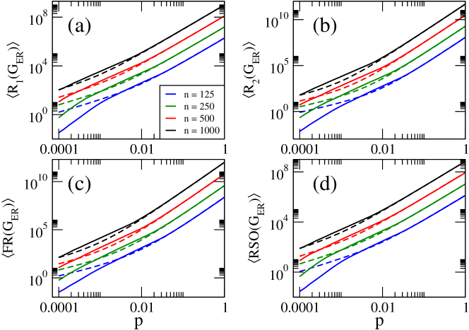
Figure 1: (a) $\left\langle R_{1}(G_{\mbox{\tiny ER}})\right\rangle$, (b) $\left\langle R_{2}(G_{\mbox{\tiny ER}})\right\rangle$, (c) $\left\langle FR(G_{\mbox{\tiny ER}})\right\rangle$, and (d) $\left\langle RSO(G_{\mbox{\tiny ER}})\right\rangle$ as a function of the probability $p$ of Erdős-Rényi graphs $G_{\mbox{\tiny ER}}(n,p)$ of sizes $n\in[125,1000]$. Dashed lines are (a) $\left\langle M_{1}(G_{\mbox{\tiny ER}})\right\rangle$, (b) $\left\langle M_{2}(G_{\mbox{\tiny ER}})\right\rangle$, (c) $\left\langle F(G_{\mbox{\tiny ER}})\right\rangle$, and (d) $\left\langle SO(G_{\mbox{\tiny ER}})\right\rangle$. Each data value was computed by averaging over $10^{6}$ random graphs $G_{\mbox{\tiny ER}}(n,p)$.

It is interesting to note, from Fig. 1, that $\left\langle RX_{\Sigma}(G_{\mbox{\tiny ER}})\right\rangle\approx\left\langle X_{\Sigma}(G_{\mbox{\tiny ER}})\right\rangle$ once $p>0.01$. Moreover, given that $RX_{\Sigma}(G_{\mbox{\tiny ER}})$ and $X_{\Sigma}(G_{\mbox{\tiny ER}})$ have the same functional form on $r$ and $d$, respectively, $\left\langle RX_{\Sigma}(G_{\mbox{\tiny ER}})\right\rangle\approx\left\langle X_{\Sigma}(G_{\mbox{\tiny ER}})\right\rangle$ must be the consequence of

$$\left\langle r(G_{\mbox{\tiny ER}})\right\rangle=\left\langle\Delta(G_{\mbox{\tiny ER}})\right\rangle+\left\langle\delta(G_{\mbox{\tiny ER}})\right\rangle-\left\langle d(G_{\mbox{\tiny ER}})\right\rangle\approx\left\langle d(G_{\mbox{\tiny ER}})\right\rangle,$$ (7)

for large $p$. Indeed, in Fig. 2(a) we plot $\left\langle r(G_{\mbox{\tiny ER}})\right\rangle$ (full lines) and $\left\langle d(G_{\mbox{\tiny ER}})\right\rangle$ (dashed lines) and clearly verify that $\left\langle r(G_{\mbox{\tiny ER}})\right\rangle\approx\left\langle d(G_{\mbox{\tiny ER}})\right\rangle$ for large $p$. Thus, the approximation in Eq. (7) implies that $\left\langle d(G_{\mbox{\tiny ER}})\right\rangle\approx[\left\langle\Delta(G_{\mbox{\tiny ER}})\right\rangle+\left\langle\delta(G_{\mbox{\tiny ER}})\right\rangle]/2$. This rough estimate of the mean from the max and min values is validated in Fig. 2(b) where we contrast $[\left\langle\Delta(G_{\mbox{\tiny ER}})\right\rangle+\left\langle\delta(G_{\mbox{\tiny ER}})\right\rangle]/2$ with $\left\langle d(G_{\mbox{\tiny ER}})\right\rangle$ and show that they certainly coincide for large enough $p$.

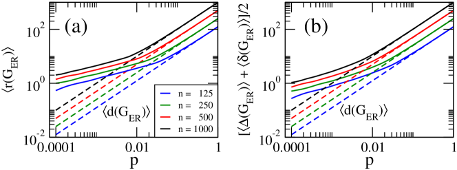
Figure 2: (a) Average Revan vertex degree $\left\langle r(G_{\mbox{\tiny ER}})\right\rangle$ and (b) $[\left\langle\Delta(G_{\mbox{\tiny ER}})\right\rangle+\left\langle\delta(G_{\mbox{\tiny ER}})\right\rangle]/2$ as a function of the probability $p$ of Erdős-Rényi graphs $G_{\mbox{\tiny ER}}(n,p)$ of sizes $n\in[125,1000]$. Dashed lines in (a,b) are the corresponding average degrees $\left\langle d(G_{\mbox{\tiny ER}})\right\rangle$. Each data value was computed by averaging over $10^{6}$ random graphs $G_{\mbox{\tiny ER}}(n,p)$.

Therefore, in the dense limit, i.e. when $\left\langle d(G_{\mbox{\tiny ER}})\right\rangle\gg 1$, we can estimate the Revan-degree--based TIs by the use of the approximations $r_{u}\approx r_{v}\approx\left\langle r(G_{\mbox{\tiny ER}})\right\rangle$ and $\left\langle d(G_{\mbox{\tiny ER}})\right\rangle\approx\left\langle r(G_{\mbox{\tiny ER}})\right\rangle$. For example, for $R_{1}(G_{\mbox{\tiny ER}})$ we can write

$$R_{1}(G_{\mbox{\tiny ER}})=\sum_{uv\in E(G_{\mbox{\tiny ER}})}r_{u}+r_{v}\approx\sum_{uv\in E(G_{\mbox{\tiny ER}})}2\left\langle r(G_{\mbox{\tiny ER}})\right\rangle\approx n\left\langle d(G_{\mbox{\tiny ER}})\right\rangle\left\langle r(G_{\mbox{\tiny ER}})\right\rangle\approx n\left\langle r(G_{\mbox{\tiny ER}})\right\rangle^{2}$$

or

$$\frac{R_{1}(G_{\mbox{\tiny ER}})}{n}\approx\left\langle r(G_{\mbox{\tiny ER}})\right\rangle^{2}.$$ (8)

Above we have used $|E(G_{\mbox{\tiny ER}})|=n\left\langle d(G_{\mbox{\tiny ER}})\right\rangle/2$. Similar approximations give

$$\frac{R_{2}(G_{\mbox{\tiny ER}})}{n}\approx\frac{1}{2}\left\langle r(G_{\mbox{\tiny ER}})\right\rangle^{3},$$ (9)

$$\frac{FR(G_{\mbox{\tiny ER}})}{n}\approx\left\langle r(G_{\mbox{\tiny ER}})\right\rangle^{3},$$ (10)

and

$$\frac{RSO(G_{\mbox{\tiny ER}})}{n}\approx\frac{1}{\sqrt{2}}\left\langle r(G_{\mbox{\tiny ER}})\right\rangle^{2}.$$ (11)

From Eqs. (8-11) we can see that the ratio $RX_{\Sigma}(G_{\mbox{\tiny ER}})/n$ should depend on $\left\langle r(G_{\mbox{\tiny ER}})\right\rangle$ only in the dense limit.

Then, in Fig. 3 we plot $\left<RX_{\Sigma}(G_{\mbox{\tiny ER}})\right>/n$ vs. $\left<r(G_{\mbox{\tiny ER}})\right>$ (full lines) and observe a good correspondence with Eqs. (8-11) (orange dashed lines) in the dense limit, i.e. when $\left\langle r(G_{\mbox{\tiny ER}})\right\rangle\geq 10$. Furthermore, except for a small-size effect evident at small $\left<r(G_{\mbox{\tiny ER}})\right>$, we notice that the curves $\left<RX_{\Sigma}(G_{\mbox{\tiny ER}})\right>/n$ vs. $\left<r(G_{\mbox{\tiny ER}})\right>$ do not depend on $n$ (that is, the curves for different graph sizes fall one on top of the other) even for $\left\langle r(G_{\mbox{\tiny ER}})\right\rangle<10$. Therefore, a scaling relation for $\left<RX_{\Sigma}(G_{\mbox{\tiny ER}})\right>$ can be stated as

$$\frac{\left<RX_{\Sigma}(G_{\mbox{\tiny ER}})\right>}{n}\approx g_{\Sigma}(\left<r(G_{\mbox{\tiny ER}})\right>)\,.$$ (12)

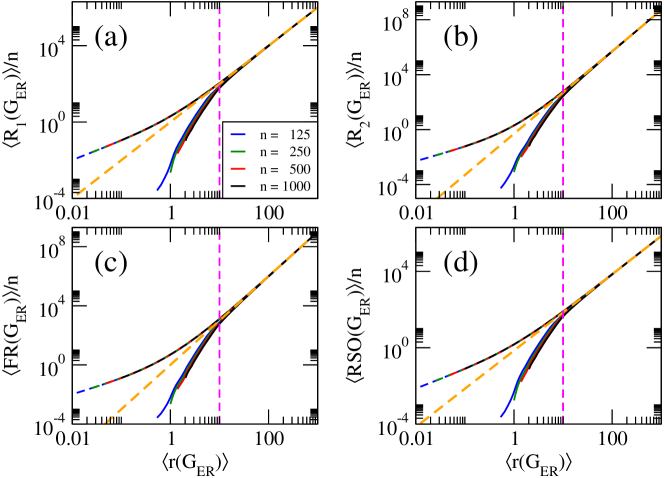
Figure 3: (a) $\left\langle R_{1}(G_{\mbox{\tiny ER}})\right\rangle/n$, (b) $\left\langle R_{2}(G_{\mbox{\tiny ER}})\right\rangle/n$, (c) $\left\langle FR(G_{\mbox{\tiny ER}})\right\rangle/n$, and (d) $\left\langle RSO(G_{\mbox{\tiny ER}})\right\rangle/n$ as a function of the average Revan vertex degree $\left\langle r(G_{\mbox{\tiny ER}})\right\rangle$ of Erdős-Rényi graphs $G_{\mbox{\tiny ER}}(n,p)$ of sizes $n\in[125,1000]$. Dashed lines are (a) $\left\langle M_{1}(G_{\mbox{\tiny ER}})\right\rangle/n$, (b) $\left\langle M_{2}(G_{\mbox{\tiny ER}})\right\rangle/n$, (c) $\left\langle F(G_{\mbox{\tiny ER}})\right\rangle/n$, and (d) $\left\langle SO(G_{\mbox{\tiny ER}})\right\rangle/n$ as a function of the average degree $\left\langle d(G_{\mbox{\tiny ER}})\right\rangle$. Same data of Fig. 1. Orange dashed lines are (a) Eq. (8), (b) Eq. (9), (c) Eq. (10), and (d) Eq. (11). The vertical magenta dashed lines indicate $\left\langle r(G_{\mbox{\tiny ER}})\right\rangle=10$.

Note that scaling (12) is the Revan version of scaling (3). Also note that in those expressions we deliberately named the functions on the rhs as $g_{\Sigma}$ and $f_{\Sigma}$, respectively, to stress that they are different. Nevertheless, as can be clearly seen in Fig. 3 where we also include the curves $\left<X_{\Sigma}(G_{\mbox{\tiny ER}})\right>/n$ vs. $\left<d(G_{\mbox{\tiny ER}})\right>$ (dashed lines), once $\left\langle r(G_{\mbox{\tiny ER}})\right\rangle\geq 10$ the curves $\left<X_{\Sigma}(G_{\mbox{\tiny ER}})\right>/n$ vs. $\left<d(G_{\mbox{\tiny ER}})\right>$ and $\left<RX_{\Sigma}(G_{\mbox{\tiny ER}})\right>/n$ vs. $\left<r(G_{\mbox{\tiny ER}})\right>$ coincide. This means that Eqs. (8-11) with $RX\to X$ and $r\to d$ also describe the corresponding degree--based indices $X_{\Sigma}(G_{\mbox{\tiny ER}})$ when $\left\langle d(G_{\mbox{\tiny ER}})\right\rangle\geq 10$; or equivalently, the functions $f_{\Sigma}$ and $g_{\Sigma}$ in the scalings (3) and (12), respectively, must be equal in the dense limit.

2.2 Revan-degree--based TIs on random geometric graphs

Now, in Fig. 4 we present the average values of the Revan-degree--based TIs $R_{1}(G_{\mbox{\tiny RG}})$, $R_{2}(G_{\mbox{\tiny RG}})$, $FR(G_{\mbox{\tiny RG}})$ and $RSO(G_{\mbox{\tiny RG}})$ as a function of the connection radius $\ell$ of RG graphs of four different sizes $n$ (full lines). In this figure we also include the corresponding average degree--based TIs as dashed lines. In addition, in Figs. 5(a) and 5(b) we plot $\left\langle r(G_{\mbox{\tiny RG}})\right\rangle$ (full lines) and $[\left\langle\Delta(G_{\mbox{\tiny RG}})\right\rangle+\left\langle\delta(G_{\mbox{\tiny RG}})\right\rangle]/2$ (full lines) as a function of $\ell$, respectively.

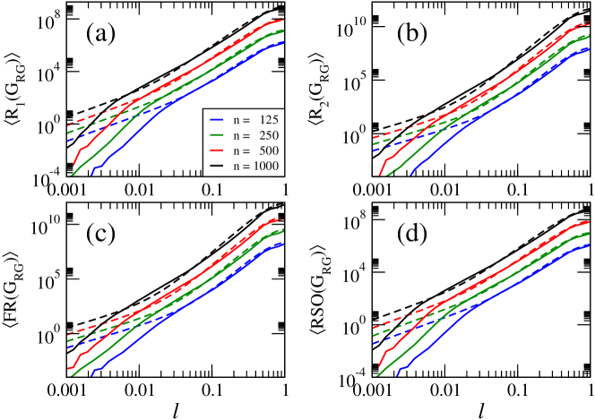
Figure 4: (a) $\left\langle R_{1}(G_{\mbox{\tiny RG}})\right\rangle$, (b) $\left\langle R_{2}(G_{\mbox{\tiny RG}})\right\rangle$, (c) $\left\langle FR(G_{\mbox{\tiny RG}})\right\rangle$, and (d) $\left\langle RSO(G_{\mbox{\tiny RG}})\right\rangle$ as a function of the connection radius $\ell$ of random geometric graphs $G_{\mbox{\tiny RG}}(n,\ell)$ of sizes $n\in[125,1000]$. Dashed lines are (a) $\left\langle M_{1}(G_{\mbox{\tiny RG}})\right\rangle$, (b) $\left\langle M_{2}(G_{\mbox{\tiny RG}})\right\rangle$, (c) $\left\langle F(G_{\mbox{\tiny RG}})\right\rangle$, and (d) $\left\langle SO(G_{\mbox{\tiny RG}})\right\rangle$. Each data value was computed by averaging over $10^{6}$ random graphs $G_{\mbox{\tiny RG}}(n,\ell)$.

Figure 5: (a) Average Revan vertex degree $\left\langle r(G_{\mbox{\tiny RG}})\right\rangle$ and (b) $[\left\langle\Delta(G_{\mbox{\tiny RG}})\right\rangle+\left\langle\delta(G_{\mbox{\tiny RG}})\right\rangle]/2$ as a function of the connection radius $\ell$ of random geometric graphs $G_{\mbox{\tiny RG}}(n,\ell)$ of sizes $n\in[125,1000]$. Dashed lines are the corresponding average degrees $\left\langle d(G_{\mbox{\tiny RG}})\right\rangle$. Each data value was computed by averaging over $10^{6}$ random graphs $G_{\mbox{\tiny RG}}(n,\ell)$.

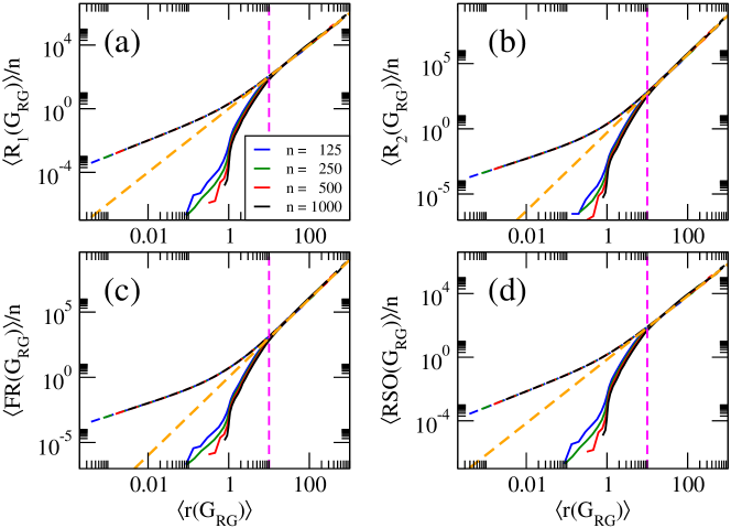
Figure 6: (a) $\left\langle R_{1}(G_{\mbox{\tiny RG}})\right\rangle/n$, (b) $\left\langle R_{2}(G_{\mbox{\tiny RG}})\right\rangle/n$, (c) $\left\langle FR(G_{\mbox{\tiny RG}})\right\rangle/n$, and (d) $\left\langle RSO(G_{\mbox{\tiny RG}})\right\rangle/n$ as a function of the average Revan vertex degree $\left\langle r(G_{\mbox{\tiny RG}})\right\rangle$ of random geometric graphs $G_{\mbox{\tiny RG}}(n,\ell)$ of sizes $n\in[125,1000]$. Dashed lines are (a) $\left\langle M_{1}(G_{\mbox{\tiny RG}})\right\rangle/n$, (b) $\left\langle M_{2}(G_{\mbox{\tiny RG}})\right\rangle/n$, (c) $\left\langle F(G_{\mbox{\tiny RG}})\right\rangle/n$, and (d) $\left\langle SO(G_{\mbox{\tiny RG}})\right\rangle/n$ as a function of the average degree $\left\langle d(G_{\mbox{\tiny RG}})\right\rangle$. Same data of Fig. 4. Orange dashed lines are (a) Eq. (8), (b) Eq. (9), (c) Eq. (10), and (d) Eq. (11) with $G_{\mbox{\tiny ER}}\to G_{\mbox{\tiny RG}}$. The vertical magenta dashed lines indicate $\left\langle r(G_{\mbox{\tiny RG}})\right\rangle=10$.

For comparison purposes, Figs. 1 and 2 for ER graphs are equivalent to Figs. 4 and 5 for RG graphs. In fact, all observations and conclusions made in the previous Subsection for ER graphs are also valid for RG graphs, namely:

• $\left\langle RX_{\Sigma}(G_{\mbox{\tiny RG}})\right\rangle\approx\left\langle X_{\Sigma}(G_{\mbox{\tiny RG}})\right\rangle$ for large $\ell$, see Fig. 4,

• $\left\langle d(G_{\mbox{\tiny RG}})\right\rangle\approx[\left\langle\Delta(G_{\mbox{\tiny RG}})\right\rangle+\left\langle\delta(G_{\mbox{\tiny RG}})\right\rangle]/2$ for large $\ell$, see Fig. 5(b), thus

• $\left\langle r(G_{\mbox{\tiny RG}})\right\rangle\approx\left\langle d(G_{\mbox{\tiny RG}})\right\rangle$ for large $\ell$, see Fig. 5(a). Therefore,

• Eqs. (8-11) with $G_{\mbox{\tiny ER}}\to G_{\mbox{\tiny RG}}$ should also be valid for RG graphs in the dense limit. This is indeed verified in Fig. 6 where we have plotted $\left<RX_{\Sigma}(G_{\mbox{\tiny RG}})\right>/n$ vs. $\left<r(G_{\mbox{\tiny RG}})\right>$ (full lines) together with Eqs. (8-11) (orange dashed lines).

• Finally, from Fig. 6, the scaling law

  $$\frac{\left<RX_{\Sigma}(G_{\mbox{\tiny RG}})\right>}{n}\approx g_{\Sigma}(\left<r(G_{\mbox{\tiny RG}})\right>)$$ (13)

  can be stated.

3 Statistical analysis of Revan-degree--based MTIs on random graphs

We now introduce the multiplicative versions of the Revan-degree--based TIs, $RX_{\Pi}(G)$, studied in the previous Section:

$$R_{1\Pi}(G)=\prod_{uv\in E(G)}r_{u}+r_{v}\,,\qquad R_{2\Pi}(G)=\prod_{uv\in E(G)}r_{u}r_{v}\,,$$

$$FR_{\Pi}(G)=\prod_{uv\in E(G)}r_{u}^{2}+r_{v}^{2}\,,$$

and

$$RSO_{\Pi}(G)=\prod_{uv\in E(G)}\sqrt{r_{u}^{2}+r_{v}^{2}}\,.$$

These MTIs are the Revan versions of the multiplicative Zagreb indices [18, 19]

$$\Pi_{1}^{*}(G)=\prod_{uv\in E(G)}d_{u}+d_{v}\,,\qquad\Pi_{2}(G)=\prod_{uv\in E(G)}d_{u}d_{v}\,,$$

the multiplicative forgotten index

$$F_{\Pi}(G)=\prod_{uv\in E(G)}d_{u}^{2}+d_{v}^{2}\,,$$ (14)

and the multiplicative Sombor index

$$SO_{\Pi}(G)=\prod_{uv\in E(G)}\sqrt{d_{u}^{2}+d_{v}^{2}}\,,$$ (15)

respectively. Note that (as far as we know) neither $F_{\Pi}(G)$ nor $SO_{\Pi}(G)$ have been considered before.

It is fair to recall that a statistical study of degree--based MTIs, $X_{\Pi}(G)$, on random graphs has been already reported in Ref. [20]. There, the multiplicative Zagreb indices, the multiplicative Randić connectivity index, the multiplicative harmonic index, the multiplicative sum-connectivity index, the multiplicative inverse degree index, as well as the Narumi-Katayama index were applied to ER graphs, RG graphs and bipartite random graphs. There it was demonstrated that $\left<\ln X_{\Pi}(G)\right>$ normalized to the order of the graph scale with the corresponding average degree:

$$\frac{\left<\ln X_{\Pi}(G)\right>}{n}\equiv f_{\Pi}(\left<d\right>)\ .$$ (16)

Note that scaling (16) can be considered as the multiplicative version of scaling (3).

Then, in what follows we apply the Revan-degree--based MTIs defined above on ER and RG graphs.

In Figs. 7 and 8 we present the average values of the Revan-degree--based MTIs $R_{1\Pi}(G)$, $R_{2\Pi}(G)$, $FR_{\Pi}(G)$ and $RSO_{\Pi}(G)$ for ER (Fig. 7) and RG (Fig. 8) graphs of four different sizes $n$ (full lines). In these figures we also plot the corresponding average degree--based MTIs as dashed lines. For both random graph models we observe that $\left\langle RX_{\Pi}(G)\right\rangle\approx\left\langle X_{\Pi}(G)\right\rangle$ for large enough $p$ and large enough $\ell$, respectively.

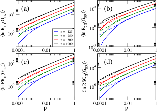
Figure 7: (a) $\left\langle\ln R_{1\Pi}(G_{\mbox{\tiny ER}})\right\rangle$, (b) $\left\langle\ln R_{2\Pi(}G_{\mbox{\tiny ER}})\right\rangle$, (c) $\left\langle\ln FR_{\Pi}(G_{\mbox{\tiny ER}})\right\rangle$, and (d) $\left\langle\ln RSO_{\Pi}(G_{\mbox{\tiny ER}})\right\rangle$ as a function of the probability $p$ of Erdős-Rényi graphs $G_{\mbox{\tiny ER}}(n,p)$ of sizes $n\in[125,1000]$. Dashed lines are (a) $\left\langle\ln\Pi^{*}_{1}(G_{\mbox{\tiny ER}})\right\rangle$, (b) $\left\langle\ln\Pi_{2}(G_{\mbox{\tiny ER}})\right\rangle$, (c) $\left\langle\ln F_{\Pi}(G_{\mbox{\tiny ER}})\right\rangle$, and (d) $\left\langle\ln SO_{\Pi}(G_{\mbox{\tiny ER}})\right\rangle$. Each data value was computed by averaging over $10^{6}$ random graphs $G_{\mbox{\tiny ER}}(n,p)$.

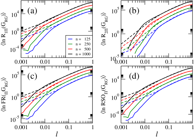
Figure 8: (a) $\left\langle\ln R_{1\Pi}(G_{\mbox{\tiny RG}})\right\rangle$, (b) $\left\langle\ln R_{2\Pi}(G_{\mbox{\tiny RG}})\right\rangle$, (c) $\left\langle\ln FR_{\Pi}(G_{\mbox{\tiny RG}})\right\rangle$, and (d) $\left\langle\ln RSO_{\Pi}(G_{\mbox{\tiny RG}})\right\rangle$ as a function of the connection radius $\ell$ of random geometric graphs $G_{\mbox{\tiny RG}}(n,\ell)$ of sizes $n\in[125,1000]$. Dashed lines are (a) $\left\langle\ln\Pi^{*}_{1}(G_{\mbox{\tiny RG}})\right\rangle$, (b) $\left\langle\ln\Pi_{2}(G_{\mbox{\tiny RG}})\right\rangle$, (c) $\left\langle\ln F_{\Pi}(G_{\mbox{\tiny RG}})\right\rangle$, and (d) $\left\langle\ln SO_{\Pi}(G_{\mbox{\tiny RG}})\right\rangle$. Each data value was computed by averaging over $10^{6}$ random graphs $G_{\mbox{\tiny RG}}(n,\ell)$.

Indeed, as for the Revan-degree--based TIs, here we can also estimate the Revan-degree--based MTIs in the dense limit by the use of the approximations $r_{u}\approx r_{v}\approx\left\langle r(G)\right\rangle$ and $\left\langle d(G)\right\rangle\approx\left\langle r(G)\right\rangle$. Thus, for $R_{1\Pi}(G)$ we write

$$R_{1\Pi}(G)=\prod_{uv\in E(G)}r_{u}+r_{v}\approx\prod_{uv\in E(G)}2\left\langle r(G)\right\rangle\approx[2\left\langle r(G)\right\rangle]^{n\left\langle d(G)\right\rangle/2}$$

which leads to

$$\ln R_{1\Pi}(G)\approx\frac{1}{2}n\left\langle d(G)\right\rangle\ln[2\left\langle r(G)\right\rangle]\approx\frac{1}{2}n\left\langle r(G)\right\rangle\ln[2\left\langle r(G)\right\rangle]$$

or

$$\frac{\ln R_{1\Pi}(G)}{n}\approx\frac{1}{2}\left\langle r(G)\right\rangle\ln[2\left\langle r(G)\right\rangle].$$ (17)

Similar approximations give

$$\frac{\ln R_{2\Pi}(G)}{n}\approx\left\langle r(G)\right\rangle\ln\left\langle r(G)\right\rangle,$$ (18)

$$\frac{\ln FR_{\Pi}(G)}{n}\approx\left\langle r(G)\right\rangle\ln[\sqrt{2}\left\langle r(G)\right\rangle],$$ (19)

and

$$\frac{\ln RSO_{\Pi}(G)}{n}\approx\frac{1}{2}\left\langle r(G)\right\rangle\ln[\sqrt{2}\left\langle r(G)\right\rangle].$$ (20)

Note that Eqs. (17-20) should work for both ER and RG graphs.

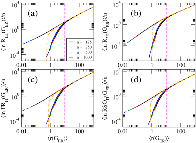
Figure 9: (a) $\left\langle\ln R_{1\Pi}(G_{\mbox{\tiny ER}})\right\rangle/n$, (b) $\left\langle\ln R_{2\Pi}(G_{\mbox{\tiny ER}})\right\rangle/n$, (c) $\left\langle\ln FR_{\Pi}(G_{\mbox{\tiny ER}})\right\rangle/n$, and (d) $\left\langle\ln RSO_{\Pi}(G_{\mbox{\tiny ER}})\right\rangle/n$ as a function of the average Revan vertex degree $\left\langle r(G_{\mbox{\tiny ER}})\right\rangle$ of Erdős-Rényi graphs $G_{\mbox{\tiny ER}}(n,p)$ of sizes $n\in[125,1000]$. Dashed lines are (a) $\left\langle\ln\Pi^{*}_{1}(G_{\mbox{\tiny ER}})\right\rangle/n$, (b) $\left\langle\ln\Pi_{2}(G_{\mbox{\tiny ER}})\right\rangle/n$, (c) $\left\langle\ln F_{\Pi}(G_{\mbox{\tiny ER}})\right\rangle/n$, and (d) $\left\langle\ln SO_{\Pi}(G_{\mbox{\tiny ER}})\right\rangle/n$ as a function of the average degree $\left\langle d(G_{\mbox{\tiny ER}})\right\rangle$. Same data of Fig. 7. Orange dashed lines are (a) Eq. (17), (b) Eq. (18), (c) Eq. (19), and (d) Eq. (20). The vertical magenta dashed lines indicate $\left\langle r(G_{\mbox{\tiny ER}})\right\rangle=10$.

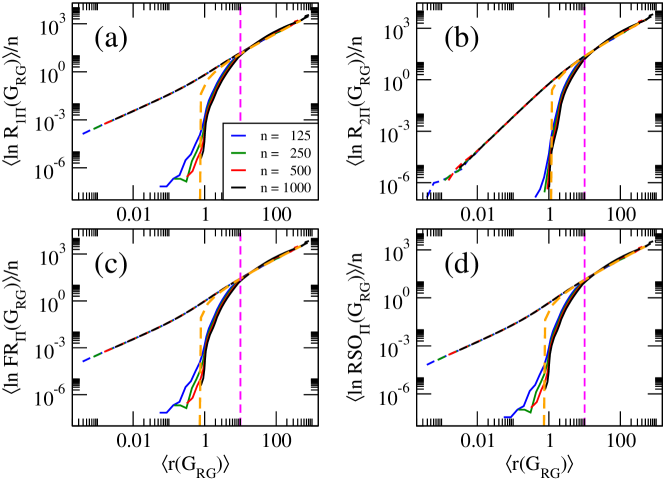
Figure 10: (a) $\left\langle\ln R_{1\Pi}(G_{\mbox{\tiny RG}})\right\rangle/n$, (b) $\left\langle\ln R_{2\Pi}(G_{\mbox{\tiny RG}})\right\rangle/n$, (c) $\left\langle\ln FR_{\Pi}(G_{\mbox{\tiny RG}})\right\rangle/n$, and (d) $\left\langle\ln RSO_{\Pi}(G_{\mbox{\tiny RG}})\right\rangle/n$ as a function of the average Revan vertex degree $\left\langle r(G_{\mbox{\tiny RG}})\right\rangle$ of random geometric graphs $G_{\mbox{\tiny RG}}(n,\ell)$ of sizes $n\in[125,1000]$. Dashed lines are (a) $\left\langle\ln\Pi^{*}_{1}(G_{\mbox{\tiny RG}})\right\rangle/n$, (b) $\left\langle\ln\Pi_{2}(G_{\mbox{\tiny RG}})\right\rangle/n$, (c) $\left\langle\ln F_{\Pi}(G_{\mbox{\tiny RG}})\right\rangle/n$, and (d) $\left\langle\ln SO_{\Pi}(G_{\mbox{\tiny RG}})\right\rangle/n$ as a function of the average degree $\left\langle d(G_{\mbox{\tiny RG}})\right\rangle$. Same data of Fig. 8. Orange dashed lines are (a) Eq. (17), (b) Eq. (18), (c) Eq. (19), and (d) Eq. (20). The vertical magenta dashed lines indicate $\left\langle r(G_{\mbox{\tiny RG}})\right\rangle=10$.

Therefore, in Figs. 9 and 10 we plot $\left<RX_{\Pi}(G)\right>/n$ vs. $\left<r(G)\right>$ (full lines) for ER and RG graphs, respectively, together with Eqs. (17-20) (orange dashed lines). Indeed, we observe a very good correspondence between predictions (17-20) and the numerical data for both random graph models in dense limit, i.e. when $\left\langle r(G)\right\rangle\geq 10$. From these figures, except for a small-size effect at small $\left<r(G_{\mbox{\tiny ER}})\right>$, we can state the scaling of the Revan-degree--based MTIs as

$$\frac{\left<\ln RX_{\Pi}(G)\right>}{n}\approx g_{\Pi}(\left<r(G)\right>)\,.$$ (21)

Note that scalings (16) and (21) indeed coincide for $\left\langle r(G)\right\rangle\geq 10$ as can be clearly seen in Figs. 9 and 10 where we also include the curves $\left<X_{\Pi}(G_{\mbox{\tiny ER}})\right>/n$ vs. $\left<d(G_{\mbox{\tiny ER}})\right>$ (dashed lines). This means that Eqs. (17-20) with $RX\to X$ and $r\to d$ also describe the corresponding degree--based indices $X_{\Pi}(G)$ when $\left\langle d(G)\right\rangle\geq 10$; or equivalently, the functions $f_{\Pi}$ and $g_{\Pi}$ in the scalings (16) and (21), respectively, must be equal in the dense limit.

4 Summary

Motivated by potential theoretical--practical applications of topological indices, in this work we perform a thorough numerical study of two families of Revan-degree--based graph invariants: $RX_{\Sigma}(G)=\sum_{uv\in E(G)}F(r_{u},r_{v})$ and $RX_{\Pi}(G)=\prod_{uv\in E(G)}F(r_{u},r_{v})$. In particular while $RX_{\Sigma}(G)$ has gained interest recently, see e.g. Refs. [7, 8, 9, 10], we are introducing $RX_{\Pi}(G)$ here. Specifically, we have considered the Revan-degree--based versions of the first and second Zagrev indices, the forgotten index, and the Sombor index. We have applied both $X_{\Sigma}(G)$ and $X_{\Pi}(G)$ on ensembles of Erdös-Rényi graphs and random geometric graphs, see Figs. 1, 4, 7 and 8.

We would like to add that we have also introduced here the multiplicative forgotten index $F_{\Pi}(G)$ and the multiplicative Sombor index $SO_{\Pi}(G)$, see Eqs. (14) and (15), respectively.

On the one hand we have shown that $\left<RX_{\Sigma}(G)\right>$ and $\left<\ln RX_{\Pi}(G)\right>$, normalized to the order of the graph $n$, scale with the average Revan degree $\left<r\right>$; that is,

$$\frac{\left<RX_{\Sigma}(G)\right>}{n}\approx g_{\Sigma}(\left<r(G)\right>)\qquad\mbox{and}\qquad\frac{\left<\ln RX_{\Pi}(G)\right>}{n}\approx g_{\Pi}(\left<r(G)\right>)\,,$$ (22)

see Figs. 3, 6, 9 and 10. On the the other hand we have provided expressions for both $\left<RX_{\Sigma}(G)\right>$ and $\left<\ln RX_{\Pi}(G)\right>$ in the dense graph limit, see Eqs. (8-11) and Eqs. (17-20), respectively.

In addition, we have found that $\left\langle r(G)\right\rangle\approx\left\langle d(G)\right\rangle$ and $\left\langle RX_{\Sigma}(G)\right\rangle\approx\left\langle X_{\Sigma}(G)\right\rangle$ in the dense limit, i. e. when $\left\langle r(G)\right\rangle\geq 10$. This makes the scalings in (22) to reproduce the scalings (3) and (16) reported in Refs. [2, 3, 4, 5, 6] and [20], respectively. Therefore, Eqs. (8-11) and Eqs. (17-20) also describe the corresponding degree-based topological indices in the dense limit. Furthermore, it is relevant to stress that the clear difference between Revan-degree--based indices and degree--based indices for $\left\langle r(G)\right\rangle<10$, makes Revan-degree--based indices particularly useful in that regime where they could provide additional information to standard degree--based indices.

We hope that our study may motivate further computational as well as theoretical studies of Revan-degree--based topological indices.