STaSy: Score-based Tabular data Synthesis

Abstract

Tabular data synthesis is a long-standing research topic in machine learning. Many different methods have been proposed over the past decades, ranging from statistical methods to deep generative methods. However, it has not always been successful due to the complicated nature of real-world tabular data. In this paper, we present a new model named Score-based Tabular data Synthesis (STaSy) and its training strategy based on the paradigm of score-based generative modeling. Despite the fact that score-based generative models have resolved many issues in generative models, there still exists room for improvement in tabular data synthesis. Our proposed training strategy includes a self-paced learning technique and a fine-tuning strategy, which further increases the sampling quality and diversity by stabilizing the denoising score matching training. Furthermore, we also conduct rigorous experimental studies in terms of the generative task trilemma: sampling quality, diversity, and time. In our experiments with 15 benchmark tabular datasets and 7 baselines, our method outperforms existing methods in terms of task-dependant evaluations and diversity. Code is available at https://github.com/JayoungKim408/STaSy.

1 Introduction

Table 1: Summary of experimental results. We report the average sampling quality and diversity scores, and time.

Methods		Quality $\uparrow$		Diversity $\uparrow$		Runtime $\downarrow$
		(F1 & $R^{2}$)		(coverage)		(second)
VEEGAN		0.006		0.038		0.109
CTGAN		0.569		0.352		0.704
TableGAN		0.501		0.434		0.046
OCT-GAN		0.567		0.381		26.926
RNODE		0.490		0.328		13.392
Naïve-STaSy		0.717		0.637		8.855
STaSy		0.733		0.658		10.663

Tabular data synthesis is of non-trivial importance in real-world applications for various reasons: protecting the privacy of original tabular data by releasing fake tabular data (Park et al., 2018; Lee et al., 2021), augmenting the original tabular data with fake data for better training machine learning models (Chawla et al., 2002; Han et al., 2005; He et al., 2008; Kim et al., 2022), and so on. However, it is well-known that tabular data frequently has such peculiar characteristics that deep generative models are not able to synthesize all possible details of the original tabular data  (Park et al., 2018; Xu et al., 2019) — given a set of columns in tabular data, columns typically follow unpredictable (multi-modal) distributions and therefore, it is hard to model their joint probability.

A couple of recent methods, however, showed remarkable successes (with some failure cases) in synthesizing fake tabular data, such as CTGAN (Xu et al., 2019), TVAE (Xu et al., 2019), IT-GAN (Lee et al., 2021), and OCT-GAN (Kim et al., 2021). In addition, a recent generative model paradigm, called score-based generative modeling (SGMs), successfully resolves the two problems of the generative learning trilemma (Xiao et al., 2021), i.e., score-based generative models provide high sampling quality and diversity, although their training/sampling time is relatively longer than other deep generative models. In this paper, we adopt a score-based generative modeling paradigm and design a Score-based Tabular data Synthesis (STaSy) method.

Our model designs significantly outperform all existing baselines in terms of the sampling quality and diversity (cf. Naïve-STaSy and STaSy in Table 1) — Naïve-STaSy is a naive conversion of SGMs toward tabular data, and STaSy additionally uses our proposed self-paced learning and fine-tuning methods. However, Figure 1 shows the difficulty of training Naïve-STaSy. The uneven and long-tailed loss distribution of Naïve-STaSy at the end of its training process means that the training is not stable for some records in training tabular data. In contrast, STaSy with our two proposed training methods yields many loss values around the left corner (i.e., close to 0).

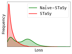
Figure 1: Distributions of denoising score matching loss in Shoppers

In order to alleviate the training difficulty of Naïve-STaSy, we design i) a self-paced learning method, and ii) a fine-tuning approach. Our proposed self-paced learning technique trains a model from easy to hard records based on their loss values. In addition, our proposed fine-tuning method, which modestly adjusts the model parameters, can further improve the sampling quality and diversity.

In Table 1, we summarize our experimental results, where we compare our STaSy with other existing tabular data synthesis methods in terms of the sampling quality, diversity, and time. As shown, our basic model even without our proposed self-paced learning and fine-tuning, denoted Naïve-STaSy, significantly outperforms all baselines except for runtime.

In summary, our contributions are as follows: i) We design a score-based generative model for tabular data synthesis. ii) We alleviate the training difficulty of the denoising score matching loss by designing a self-paced learning strategy and further enhance the sampling quality and diversity using a proposed fine-tuning method. STaSy, thus, clearly balances among the generative learning trilemma: sampling quality, diversity, and time. iii) Our proposed method outperforms other deep learning methods in all cases by large margins, which we consider a significant advance in the field of tabular data synthesis. iv) We evaluate various methods in terms of the generative learning trilemma in a rigorous manner.

2 Related work

2.1 Score-based generative models

Score-based generative models (SGMs) use a diffusion process defined by the following Itô stochastic differential equation (SDE):

$$d\mathbf{x}=\mathbf{f}(\mathbf{x},t)dt+g(t)d\mathbf{w},$$ (1)

where $\mathbf{f}(\mathbf{x},t)=f(t)\mathbf{x}$, $f$ and $g$ are drift and diffusion coefficients of $\mathbf{x}(t)$, and $\mathbf{w}$ is the standard Wiener process. Depending on the types of $f$ and $g$, SGMs can be divided into variance exploding (VE), variance preserving (VP), and sub-variance preserving (sub-VP) models (Song et al., 2021). The definitions of $f$ and $g$ are in Appendix A. The reverse of the diffusion process is a denoising process as follows:

$$d\mathbf{x}=\big{(}\mathbf{f}(\mathbf{x},t)-g^{2}(t)\nabla_{\mathbf{x}}\log p_{t}(\mathbf{x})\big{)}dt+g(t)d\mathbf{w},$$ (2)

where this reverse SDE is a process of generating samples. The score function $\nabla_{\mathbf{x}}\log p_{t}(\mathbf{x})$ is approximated by a time-dependent score-based model $S_{\bm{\theta}}(\mathbf{x},t)$, called score network.

In general, following the diffusion process in Equation 1, we can derive $\mathbf{x}(t)$ at time $t\in[0,T]$, where $\mathbf{x}(0)$ and $\mathbf{x}(T)$ means a real and noisy sample, respectively. The transition probability $p(\mathbf{x}(t)|\mathbf{x}(0))$ at time $t$ is easily approximated by this process, and it always follows a Gaussian distribution. It allows us to collect the gradient of the log transition probability, $\nabla_{\mathbf{x}(t)}\log p(\mathbf{x}(t)|\mathbf{x}(0))$, during the diffusion process. Therefore, we can train a score network $S_{\bm{\theta}}(\mathbf{x},t)$ as follows:

$$\operatorname*{arg\,min}_{\bm{\theta}}\mathbb{E}_{t}\mathbb{E}_{\mathbf{x}(t)}\mathbb{E}_{\mathbf{x}(0)}\Big{[}\lambda(t)\|S_{\bm{\theta}}(\mathbf{x}(t),t)-\nabla_{\mathbf{x}(t)}\log p(\mathbf{x}(t)|\mathbf{x}(0))\|_{2}^{2}\Big{]},$$ (3)

where $\lambda(t)$ is to control the trade-off between the sampling quality and likelihood. This is called the denoising score matching, and $\bm{\theta}^{*}$ solving Equation 3 can accurately solve the reverse SDE in Equation 2 (Vincent, 2011).

After the training process, we can synthesize fake data records with i) the predictor-corrector framework or ii) the probability flow method, a deterministic method based on the ordinary differential equation (ODE) whose marginal distribution is equal to that of  Equation 1 (Song et al., 2021). In particular, the latter enables fast sampling and exact log-probability computation.

2.2 Tabular data synthesis

Many distinct methods exist for tabular data synthesis, which creates realistic synthetic tables depending on the data types. For example, a recursive table modeling utilizing a Gaussian copula is used to synthesize continuous variables (Patki et al., 2016). Discrete variables can be generated by Bayesian networks (Zhang et al., 2017; Aviñó et al., 2018) and decision trees (Reiter, 2005). Several data synthesis methods based on GANs have been presented to generate tabular data in recent years. RGAN (Esteban et al., 2017) creates continuous time-series healthcare records, whereas MedGAN (Choi et al., 2017) and corrGAN (Patel et al., 2018) generate discrete records. EhrGAN (Che et al., 2017) utilizes semi-supervised learning to generate plausible labeled records to supplement limited training data. PATE-GAN (Jordon et al., 2019) generates synthetic data without jeopardizing the privacy of real data. TableGAN (Park et al., 2018) employs convolutional neural networks to enhance tabular data synthesis and maximize label column prediction accuracy. CTGAN and TVAE (Xu et al., 2019) adopt column-type-specific preprocessing steps to deal with multi-modality in the original dataset distribution. OCT-GAN (Kim et al., 2021) is a generative model design based on neural ODEs. SOS (Kim et al., 2022) proposed a style-transfer-based oversampling method for imbalanced tabular data using SGMs, whose main strategy is converting a major sample to a minor sample. Since its task is not compatible to our task to generate from the scratch, direct comparisons are not possible. However, we convert our method to an oversampling method following their design guidance and compare with SOS in Appendix B.

2.3 Self-paced learning

Self-paced learning (SPL) is a training strategy related to curriculum learning to select training records in a meaningful order, inspired by the learning process of humans (Kumar et al., 2010b; Jiang et al., 2014). It refers to training a model only with a subset of data that has low training losses and gradually expanding to the entire training data. We denote the training set as $\mathcal{D}=\{\mathbf{x}_{i}\}^{N}_{i=1}$, where $\mathbf{x}_{i}$ is the $i$-th record. The model $M$ with parameters $\bm{\theta}$ has a loss $l_{i}=L(M(\mathbf{x}_{i},\bm{\theta}))$, where $L$ is the loss function. A vector $\mathbf{v}=[v_{i}]^{N}_{i=1},v_{i}\in\{0,1\}$ indicates whether $\mathbf{x}_{i}$ is easy or not for all $i$. SPL aims to learn the model parameter $\bm{\theta}$ and the selection importance $\mathbf{v}$ by minimizing:

$$\min_{\bm{\theta},\mathbf{v}}\mathbb{E}(\bm{\theta},\mathbf{v})=\sum_{i=1}^{N}v_{i}L(M(\mathbf{x}_{i},\bm{\theta}))-\frac{1}{K}\sum_{i=1}^{N}v_{i},$$ (4)

where $K$ is a parameter to control the learning pace. In general, the second term in Equation 4, called a self-paced regularizer, can be customized for a downstream task.

The alternative convex search (ACS) (Bazaraa et al., 1993) is typically used to solve Equation 4 (Kumar et al., 2010a; Tang et al., 2012). By alternately optimizing variables while fixing others, we can optimize Equation 4, i.e., update $\mathbf{v}$ after fixing $\bm{\theta}$, and vice versa. With fixed $\bm{\theta}$, the global optimum $\mathbf{v}^{*}=[v^{*}_{i}]^{N}_{i=1}$ is defined as follows:

$$v^{*}_{i} =\begin{cases}1,&l_{i}<\frac{1}{K},\\ 0,&l_{i}\geq\frac{1}{K},\\ \end{cases}$$ (5)

When updating $\mathbf{v}$ with fixed $\bm{\theta}$, a record $\mathbf{x}_{i}$ with $l_{i}<\frac{1}{K}$ is regarded as an easy record and will be chosen for training. Only easy records are used to train the model. Otherwise, $\mathbf{x}_{i}$ is regarded as a hard record and will be unselected. To involve more records in the training process, $K$ is gradually decreased.

3 Proposed method

STaSy is an SGM-based method for tabular data synthesis. STaSy uses SPL to ensure its training stability. The suggested fine-tuning method takes advantage of a favorable property of SGMs, which is that we can measure the log-probabilities of records.

3.1 Score network architecture & miscellaneous designs

It is known that each column in tabular data typically has complicated distributions, whereas pixel values in image datasets typically follow Gaussian distributions (Xu et al., 2019). Moreover, tabular synthesis models should learn the joint probability of multiple columns to generate a record, which is one main reason why tabular data synthesis is difficult. However, one good design point is that the dimensionality of tabular data is typically far less than that of image data, e.g., 784 pixels even in MNIST, one of the simplest image datasets, vs. 30 columns in Credit.

We found through our preliminary experiments that the SDE in Equations 1 and 2 can well model the joint probability iff its score network, which approximates $\nabla_{\mathbf{x}}\log p_{t}(\mathbf{x})$, is well trained. We carefully design our score network for tabular data synthesis considering these points. Our proposed score network architecture is in Appendix C.

Since SGMs were theoretically designed from the idea of perturbing data with an infinite number of noise scales, SGMs typically require large-scale computation, e.g., $T=1,000$ for images in (Song et al., 2021), as an approximation to the infinite number. With a large number of steps, the denoising process requires a long time to complete, which is one part of the generative learning trilemma. However, we found that $T=50$ steps in Equation 1 are enough to train a network to approximate the gradient of the log-likelihood, which means that our STaSy naturally has less sampling time than SGMs for images with $T=1,000$ steps.

Pre/post-processing of tabular data To handle mixed types of data, which is a challenge in tabular data generation, we pre/post-process columns. We use the min-max scaler to pre-process numerical columns, and its reverse scaler is used for post-processing after generation. We also apply one-hot encoding to pre-process categorical columns, and use the softmax function, followed by the rounding function, when generating.

How to generate After sampling a noisy vector $\mathbf{z}\sim\mathcal{N}(\bm{\mu},\sigma^{2}\mathbf{I})$, the reverse SDE can convert $\mathbf{z}$ into a fake record. The prior distribution $\mathbf{z}\sim\mathcal{N}(\bm{\mu},\sigma^{2}\mathbf{I})$ varies depending on the type of SDEs: $\mathcal{N}(\mathbf{0},\sigma^{2}_{max}\mathbf{I})$ for VE, and $\mathcal{N}(\mathbf{0},\mathbf{I})$ for VP and sub-VP. $\sigma_{max}$ is a hyperparameter. In particular, we adopt the probability flow method to solve the reverse SDE, which will be shortly described in Equation 10.

3.2 Self-paced learning approach

In order to alleviate the training difficulty, we apply a curriculum learning technique for STaSy, more specifically, self-paced learning. Instead of letting $v_{i}\in\{0,1\}$, we use a “soft” record sampling method, i.e., $v_{i}\in[0,1]$. If $l_{i}$, which is the denoising score matching objective on $i$-th record, is less than a threshold, we set $v_{i}$ to 1 to ensure that the record is fully involved in training. At the end of the training, $v_{i}$ must be set to 1 for all $i$ to train the model with the entire data. The denoising score matching loss for $i$-th training record $\mathbf{x}_{i}$ is defined as follows:

$$l_{i}=\mathbb{E}_{t}\mathbb{E}_{\mathbf{x}_{i}(t)}\Big{[}\lambda(t)\|S_{\bm{\theta}}(\mathbf{x}_{i}(t),t)-\nabla_{\mathbf{x}_{i}(t)}\log p(\mathbf{x}_{i}(t)|\mathbf{x}_{i}(0))\|_{2}^{2}\Big{]}.$$ (6)

Then, we have the following STaSy objective:

$$\underset{\bm{\theta},\mathbf{v}}{min}\sum_{i=1}^{N}v_{i}l_{i}+r(\mathbf{v};\alpha,\beta),$$ (7)

where $0\leq v_{i}\leq 1$ for all $i$, $r(\cdot)$ is a self-paced regularizer. $\alpha\in[0,1]$ and $\beta\in[0,1]$ are variables to define thresholds, which are monotonically increasing as training goes on (see Appendix D for their exact controlling mechanism).

Definition 1

Let $Q(p)$ be a quantile function defined as $\inf\{l\in\mathbb{R}:p\leq F(l)\}$, where $F$ is a cumulative distribution function of the denoising score matching objective. That is, $Q(p)$ is the minimum value for which the CDF is greater than or equal to the given probability $p$.

Theorem 1

Let the self-paced regularizer $r(\mathbf{v};\alpha,\beta)$ is defined as follows:

$$r(\mathbf{v};\alpha,\beta)=-\frac{Q(\alpha)-Q(\beta)}{2}\sum_{i=1}^{N}v_{i}^{2}-Q(\beta)\sum_{i=1}^{N}v_{i},$$ (8)

where the closed-form optimal solution for $\mathbf{v}^{*}=[v_{1}^{*},v_{2}^{*},\dots,v_{N}^{*}]$, given fixed $\bm{\theta}$, is defined as follows — its proof is in Appendix E:

$$v_{i}^{*}=\begin{dcases*}1,&if $l_{i}\leq Q(\alpha)$,\\ 0,&if $l_{i}\geq Q(\beta)$,\\ \frac{l_{i}-Q(\beta)}{Q(\alpha)-Q(\beta)},&otherwise.\end{dcases*}$$ (9)

Specifically, records with $l_{i}\leq Q(\alpha)$ are considered easy records and will be selected for training, whereas records with $l_{i}\geq Q(\beta)$ are considered complicated (or potentially noisy) and will not be selected. If not both cases, records will be partially selected during training, i.e., $v_{i}\in[0,1]$. $\alpha$ and $\beta$ are gradually increased to 1 from the initial values $\alpha_{0}$ and $\beta_{0}$, proportionally to training progress to ensure that all data records are involved in training. As $\alpha$ and $\beta$ increase, the difficult records are gradually involved in training, and the model also becomes more robust to those difficult cases. We set $\alpha_{0}$ and $\beta_{0}$ in such a way that more than 80% of the training records are included in the learning process from the beginning.

1

2

3Initialize $\bm{\theta},\mathbf{v}$

/* Train SGM based on our SPL training strategy */

4 for each mini-batch of records do

5      

6      Update $\bm{\theta}$ after fixing $\mathbf{v}$ with Equation 7

7      

8      Update $\mathbf{v}$ with Equation 9

9       Update $\alpha$ and $\beta$ with the control method in Appendix D

10      

/* Fine-tune the trained model using log-probability */

11

12$\tau_{i}\leftarrow\log p(\mathbf{x}_{i})$

13 $\mathcal{F}\leftarrow\{\mathbf{x}_{i}|\log p(\mathbf{x}_{i})\textrm{, where $\mathbf{x}_{i}\in\mathcal{D}$, is smaller than the average (or median) log-probability}.\}$

14 for each fine-tune epoch do

15       for each $\mathbf{x}_{i}\in\mathcal{F}$ do

16             Update $\bm{\theta}$ with Equation 6

17      $\mathcal{F}\leftarrow\{\mathbf{x}_{i}|\log p({\mathbf{x}}_{i})<{\tau}_{i}\}$

18return $\bm{\theta}$

Algorithm 1 How to train STaSy

3.3 Fine-tuning approach

For solving the reverse SDE process, score-based generative models rely on various numerical approaches. One of the techniques is the probability flow method in Equation 10 (Song et al., 2021), which uses a deterministic process whose marginal probability is the same as the SDE. With the approximated score function $S_{\bm{\theta}}(\cdot)$, the probability flow method uses the following neural ordinary differential equation (NODE) based model (Chen et al., 2018):

$$d\mathbf{x}=\big{(}\mathbf{f}(\mathbf{x},t)-{1\over 2}g(t)^{2}\nabla_{\mathbf{x}}\log p_{t}(\mathbf{x})\big{)}dt.$$ (10)

In our experiments, the probability flow shows better quality than other methods to solve the original reverse SDE, and our default solver is the probability flow (see Section 4.3). In addition, NODEs facilitate computing the log-probability defined in Equation 10 through the instantaneous change of variables theorem. Consequently, we can calculate the exact log-probability efficiently with the unbiased Hutchinson’s estimator (Hutchinson, 1989; Grathwohl et al., 2018). Thus, we propose to fine-tune based on the exact log-probability.

After learning the model parameter $\bm{\theta}$ as described in Section 3.2, we set the sample-wise threshold $\tau_{i}$ to $\log p(x_{i})$ (cf. Line 1 of Algorithm 1). We then prepare the fine-tuning candidate set $\mathcal{F}$ (cf. Line 1 of Algorithm 1). After fine-tuning for the samples in $\mathcal{F}$, we update the candidate set (cf. Line 1 of Algorithm 1). Our goal is for achieving a better log-probability than the initial one $\tau_{i}$ before the fine-tuning process.

3.4 Training algorithm

Algorithm 1 shows the overall training process for our STaSy. Firstly, we initialize the parameters of the score network $\bm{\theta}$ and the selection importance $\mathbf{v}$. Utilizing ACS, we then train STaSy with the SPL training strategy. At this step, we iteratively optimize $\bm{\theta}$ and $\mathbf{v}$. We can obtain an optimal $\bm{\theta}$ by optimizing Equation 7 with fixed $\mathbf{v}$, and the global optimum $\mathbf{v}$ is calculated by Equation 9. We also update $\alpha$ and $\beta$ in proportion to training progress. After finishing the main SPL training step, we can generate fake records from the model. However, we further improve the score network in the fine-tuning step. We retrain our model for every record $\mathbf{x}_{i}$ whose log-probabilities are less than its threshold $\tau_{i}$. At Line 1 of Algorithm 1, one can use the log-probability instead of Equation 6 as a fine-tuning objective. However, we found that Equation 6 is more effective (see Appendix F).

4 Experiments

We analyze various methods in terms of the generative learning trilemma. We list only aggregated results over all the tested datasets in the main paper, but in Appendix G detailed results with their mean and std. dev. scores from 5 different executions are reported.

4.1 Experimental environments

A brief description of our experimental environments is as follows: i) We use 15 real-world tabular datasets for classification and regression and 7 baseline methods. To be specific about our models, Naïve-STaSy is a naive conversion of SGMs without our proposed training strategies, and STaSy is trained with self-paced learning and the fine-tuning method. ii) In general, we follow the “train on synthetic, test on real (TSTR)” framework (Esteban et al., 2017; Jordon et al., 2019), which is a widely used evaluation method for tabular data (Xu et al., 2019; Kim et al., 2021; Lee et al., 2021), to evaluate the quality of sampling — in other words, we train various models, including DecisionTree, AdaBoost, Logistic/Linear Regression, MLP classifier/regressor, RandomForest, and XGBoost, with fake data and test them with real data. For Identity, we train with real training data and test with real testing data, whose score can be a criterion to evaluate the sampling quality of various generative methods in a dataset. iii) We use various metrics to evaluate in various aspects. For the sampling quality, we mainly use average F1 for classification, and also report AUROC and Weighted-F1. We use $R^{2}$ and RMSE for regression. For the sampling diversity, we use coverage (Naeem et al., 2020), which was proposed to measure the diversity of generated records. Full results are in Appendix G. Detailed environments and hyperparameter settings are in Appendix H and I, respectively.

4.2 Experimental results

Table 2: Classification/regression with real data. We report average F1 (resp. macro F1), AUROC, and Weighted-F1 for binary (resp. multi-class) classification, and $R^{2}$ and RMSE for regression. The best (resp. the second best) results are highlighted in bold face (resp. with underline).

Methods		Classification				Regression
		F1	AUROC	Weighted-F1		$R^{2}$	RMSE
Identity		0.806	0.934	0.818		0.366	4109.424
MedGAN		0.252	0.628	0.243		-inf	inf
VEEGAN		0.371	0.704	0.356		-2.369	8540.780
CTGAN		0.639	0.849	0.649		0.113	4096.279
TVAE		0.603	0.839	0.608		0.107	4218.457
TableGAN		0.582	0.836	0.586		-0.026	4535.514
OCT-GAN		0.630	0.865	0.637		0.160	4105.729
RNODE		0.545	0.839	0.550		0.130	4112.928
Naïve-STaSy		0.777	0.922	0.786		0.324	4076.596
STaSy		0.792	0.925	0.801		0.350	4071.643

4.2.1 Sampling quality

Table 2 summarizes the key results on the sampling quality. We use task-oriented metrics, such as F1, $R^{2}$, and so on, under the TSTR evaluation framework. MedGAN and VEEGAN, two early GAN-based methods, show relatively lower test scores than other GAN-based methods, i.e., CTGAN, TableGAN, and OCT-GAN. In general, CTGAN and OCT-GAN show reliable quality among the baselines. However, our two score-based models always mark the best and the second best quality.

Our methods, Naïve-STaSy and STaSy, significantly outperform all the baselines by large margins. In particular, our methods perform well in small datasets, e.g., Crowdsource, Obesity, and Robot, while other methods show poor quality, as shown in Table 14 of Appendix G.1. These multi-class classification datasets have a small number of per class record, e.g., the smallest class in Crowdsource has 79 records in the training set, which means that our methods are able to capture fine-grained modes from the original data. Moreover, in Credit, which has a severe class imbalance ratio of 99.7% for class 0 and 0.3% for class 1, more than half of the baselines failed to generate the minority class, showing an F1 score close to 0 in Table 11 of Appendix G.1. CTGAN and TableGAN also achieve a good F1 score close to that of Identity, but Naïve-STaSy and STaSy take the first and the second places again.

Table 3: The median of the log-probabilities of testing records, averaged over all datasets

Methods		Log-probability
RNODE		59.327
STaSy w/o fine-tuning		129.293
STaSy		131.734

As flow-based generative models and SGMs with the probability flow method can calculate the exact log-probability of records, we present the log-probability as another metric for the sampling quality. Table 3 shows the median of the log-probabilities of testing records, averaged over all datasets. Since the log-probability is not bounded, we take a median of them to handle the case of outliers. Our methods, even without the fine-tuning, show a much better log-probability than RNODE, which optimizes the log-probability as its objective. Moreover, the median log-probability of testing records even improves after the proposed fine-tuning method.

Putting it all together, our proposed score-based generative models, i.e., Naïve-STaSy and STaSy, show reasonable performance in all cases regarding the machine learning efficacy and log-probability. Furthermore, as shown in Tables 2 and 3, the sampling quality always improves with the proposed training strategies, i.e., the self-paced learning and the fine-tuning, which justifies their efficacy.

4.2.2 Sampling diversity

Table 4: Sampling diversity in terms of coverage averaged over all datasets

Methods		Coverage
MedGAN		0.037
VEEGAN		0.038
CTGAN		0.352
TVAE		0.494
TableGAN		0.434
OCT-GAN		0.381
RNODE		0.328
Naïve-STaSy		0.637
STaSy w/o fine-tuning		0.655
STaSy		0.658

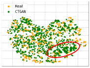
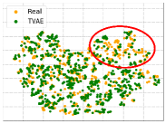
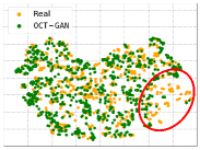
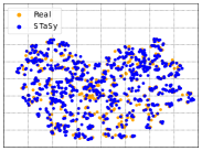
Figure 2: t-SNE visualizations of fake and the original records in Robot.

For the quantitative evaluation of the sampling diversity between existing methods and our proposed method, we use the coverage score (Naeem et al., 2020), which is bounded between 0 and 1. Coverage is the ratio of real records that have at least one fake record in its manifold. A manifold is a sphere around the sample with radius $r$, where $r$ is the distance between the sample and the $k$-th nearest neighborhood. Table 4 summarizes the averaged coverage of each method. MedGAN and VEEGAN show poor coverage scores, close to 0. This trend is also shown in the t-SNE visualizations in Appendix J.2. Among the baseline methods, CTGAN performs the best in terms of the sampling quality, whereas it shows relatively inferior coverage performance than others. In specific, in Robot, STaSy shows a coverage of 0.94, while other three top-performing baselines, CTGAN, TableGAN, and OCT-GAN, show coverage scores less than 0.26 in Table 20 of Appendix G.2. Figure 2 also presents the diversity of each fake data by each method qualitatively, which reflects the results of coverage. In general, STaSy shows stable performance across the sampling quality and the sampling diversity, outperforming others by large margins.

In Figure 3 (Left and Middle), the fake data by STaSy shows an almost identical distribution to that of real data. In contrast, OCT-GAN, which was proposed to address the multi-modality issue of tabular data, fails to do it. This means that STaSy is able to capture every mode in the columns, while OCT-GAN is not. In Figure 3 (Right), CTGAN generates some out-of-distribution records, highlighted in red.

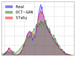
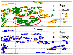
Figure 3: (Left and Middle) Histograms of values in two columns of Bean. (Right) t-SNE (van der Maaten & Hinton, 2008) visualizations of the fake and original records in Obesity. More visualizations are in Appendix J.

4.2.3 Sampling time

Table 5: Runtime evaluation results, averaged over all datasets

Methods	MedGAN	VEEGAN	CTGAN	TVAE	TableGAN	OCT-GAN	RNODE	Naïve-STaSy	STaSy
Runtime	0.246	0.109	0.704	0.100	0.046	26.926	13.392	8.855	10.663

We summarize runtime in Table 5. In order to compare the runtime of all methods, we measure the wall-clock time taken to sample $N$ records, where $N$ is training size, 5 times, and average them. In general, simple GAN-based methods, especially TableGAN and TVAE, show faster runtime. On the other hand, SGMs, OCT-GAN, and RNODE take a relatively long time for sampling. Our proposed methods, Naïve-STaSy and STaSy, take a long sampling time compared to simple GAN-based methods but are faster than OCT-GAN and RNODE, which means a well-balanced trade-off between the sampling quality, diversity, and time.

4.3 Ablation & sensitivity studies

Table 6: Ablation study. We report F1 (resp. $R^{2}$) for classification (resp. regression).

Datasets	Naïve-STaSy	w/o fine-tuning	w/o SPL	STaSy
Credit	0.782±0.042	0.782±0.044	0.790±0.028	0.794±0.035
Default	0.509±0.014	0.517±0.009	0.511±0.016	0.523±0.007
Shoppers	0.635±0.017	0.642±0.009	0.635±0.018	0.642±0.015
Contraceptive	0.418±0.018	0.437±0.012	0.434±0.015	0.451±0.017
Crowdsource	0.710±0.104	0.738±0.099	0.730±0.108	0.743±0.104
Shuttle	0.791±0.056	0.807±0.088	0.816±0.045	0.865±0.072
Beijing	0.625±0.141	0.670±0.166	0.635±0.145	0.672±0.166

Table 7: Sensitivity analyses. We report F1 (resp. $R^{2}$) for classification (resp. regression).

Datasets	SDE Type	Metric	$\alpha_{0}$	Metric	$\beta_{0}$	Metric
Spambase	VE	0.866±0.036	0.05	0.890±0.026	0.70	0.890±0.023
	VP	0.875±0.029	0.10	0.888±0.024	0.80	0.893±0.025
	sub-VP	0.893±0.025	0.30	0.888±0.027	0.90	0.890±0.028
Crowdsource	VE	0.743±0.104	0.05	0.715±0.103	0.75	0.712±0.097
	VP	0.717±0.102	0.10	0.713±0.099	0.80	0.692±0.127
	sub-VP	0.667±0.116	0.30	0.709±0.105	0.95	0.700±0.111
Beijing	VE	0.672±0.166	0.05	0.663±0.162	0.70	0.669±0.165
	VP	0.594±0.144	0.10	0.667±0.164	0.75	0.668±0.165
	sub-VP	0.525±0.082	0.30	0.666±0.164	0.95	0.668±0.165

We define three ablation models: ‘Naïve-STaSy’ without SPL and fine-tuning, ‘w/o fine-tuning’ without fine-tuning but with SPL, and ‘w/o SPL’ without SPL but with fine-tuning. All ablation models are inferior to STaSy in Table 6, showing the effectiveness of SPL and fine-tuning. In particular, SPL improves the sampling diversity as in Figure 4. Naïve-STaSy suffers from mild mode collapses, as highlighted in red.

Table 7 shows sensitivity analyses w.r.t. some important hyperparameters. In general, all settings show reasonable results, outperforming the baselines. We recommend 0.2 and 0.25 for $\alpha_{0}$ and 0.9 and 0.95 for $\beta_{0}$.

We can adopt a variety of methods to solve the reverse SDE process in Equation 2. Our method can generate fake records with the predictor-corrector framework (Pred. Corr.) or the probability flow (PF) method (Song et al., 2021). The former uses the ancestral sampling (AS), reverse diffusion (RD), or Euler-Maruyama (EM) method for solving the reverse SDE, and for the correction process, the Langevin corrector. In Table 8, the probability flow method in Equation 10 mostly leads to successful results, and other datasets also show similar results.

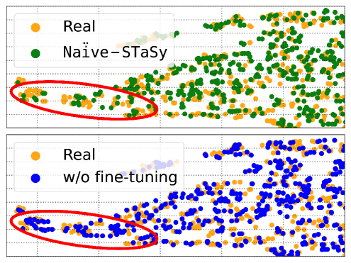
Figure 4: t-SNE visualizations of the fake and original records in Beijing

Table 8: Results of Naïve-STaSy by various reverse SDE solvers in Magic, where ‘Pred.’ means the predictor-only method. We report F1.

Predictor	Pred.	Pred. Corr.
AS	0.752±0.025	0.777±0.048
RD	0.779±0.052	0.775±0.054
EM	0.779±0.052	0.771±0.048
PF	0.781±0.054	No Corr.

5 Conclusions and discussions

Synthesizing tabular data is an important yet non-trivial task, as it requires modeling a joint probability of multi-modal columns. To this end, we presented our detailed designs and experimental results with thorough analyses. Our proposed method, STaSy, is a score-based model equipped with our proposed self-paced learning and fine-tuning methods. In our experiments with 15 benchmark datasets and 7 baselines, STaSy outperforms other deep learning methods in terms of the sampling quality and diversity (and with an acceptable sampling time). Based on these considerations, we believe that STaSy shows significant advancements in tabular data synthesis. We expect much follow-up work in utilizing SGMs for tabular data synthesis.

Limitations. Although our model shows the best balance for the deep generative task trilemma, we think that there exists room to improve runtime further — existing simple GAN-based methods are faster than our method for sampling fake records. In addition, SGMs are known to be sometimes unstable for high-dimensional data, e.g., high-resolution images, but in general, stable for low-dimensional data, e.g., tabular data. Therefore, we think that SGMs have much potential for tabular data synthesis in the future.

6 Ethics statement

Indeed, people do not always use artificial intelligence technology for righteous purposes. One can use our method to achieve his/her wrongful goals, e.g., selling high-quality fake data generated by our method, and retrieving private original data records from synthetic data. However, we believe that our research has much more beneficial points. One can use our method to generate fake data and share (after hiding the original data) to prevent potential privacy leakages. We, of course, need more studies to achieve the privacy protection goal based on our model. However, a research trend exists where researchers try to use a deep generative model to protect privacy (Park et al., 2018; Lee et al., 2021).

7 Reproducibility statement

To reproduce the experimental results, we have made the following efforts: 1) Source codes used in the experiments are available in the supplementary material. By following the README guidance, the main results are easily reproducible. 2) All the experiments are repeated five times, and their mean and standard deviation values are reported in Appendix. 3) We provide extensive experimental details in Appendix H.

Appendix A VE, VP, and sub-VP SDEs

We introduce the definitions of $f$ and $g$ as follows:

$$f(t) =\begin{cases}0,&\textrm{ if VE,}\\ -\frac{1}{2}\gamma(t)\mathbf{x},&\textrm{ if VP,}\\ -\frac{1}{2}\gamma(t)\mathbf{x},&\textrm{ if sub-VP,}\\ \end{cases}$$ (11)

$$g(t) =\begin{cases}\sqrt{\frac{\texttt{d}[\sigma^{2}(t)]}{\texttt{d}t}},&\textrm{ if VE,}\\ \sqrt{\gamma(t)},&\textrm{ if VP,}\\ \sqrt{\gamma(t)(1-e^{-2\int_{0}^{t}\gamma(s)\,\texttt{d}s})},&\textrm{ if sub-VP,}\\ \end{cases}$$ (12)

where $\sigma(t)$ and $\gamma(t)$ are noise functions w.r.t. time $t$. $\sigma(t)=\sigma_{min}\left(\frac{\sigma_{max}}{\sigma_{min}}\right)^{t}$ for $t\in[0,1]$, where $\sigma_{min}$ and $\sigma_{max}$ are hyperparameters, and we use $\sigma_{min}=\{0.01,0.1\}$ and $\sigma_{max}=\{5.0,10.0\}$. $\gamma(t)=\gamma_{min}+t\left(\gamma_{max}-\gamma_{min}\right)$ for $t\in[0,1]$, where $\gamma_{min}$ and $\gamma_{max}$ are hyperparameters, and we use $\gamma_{min}=\{0.01,0.1\}$ and $\gamma_{max}=\{5.0,10.0\}$.

Appendix B Comparison between SOS and STaSy for the oversampling task

Table 9: Comparison between SOS and STaSy in terms of Weighted-F1

Methods		HTRU		Magic		Robot
Identity		0.8657±0.0163		0.7807±0.0348		0.9031±0.0848
SOS		0.8767±0.0017		0.7949±0.0011		0.9197±0.0040
STaSy		0.8803±0.0027		0.7960±0.0015		0.9270±0.0029

In this section, we discuss the difference between SOS and STaSy. They are both based on SGMs, but they are optimized towards different goals by using different objective functions and training strategies. SOS has many design points specialized to augment minor classes only (rather than synthesizing entire tabular data) — for instance, SOS adopts a style-transfer-based idea to convert a major class sample to a minor one via their own SGM model without any consideration on the training difficulty of the denoising score matching. However, our STaSy more focuses on synthesizing entire tabular data by proposing special self-paced training and fine-tuning methods.

Since STaSy can be converted to an oversampling method following the design guidance of SOS, we conduct oversampling experiments with STaSy to compare with SOS (Kim et al., 2022). We train, for fair comparison, STaSy w/o fine-tuning for each minor class and generate minority samples to be the same size of the majority class. We compare the two models in terms of the sampling quality using Weighted-F1 which is specialized in evaluating imbalanced data. We note that Identity means that we do not use any oversampling methods, which is, therefore, a minimum quality requirement upon oversampling.

As shown in Table 9, STaSy w/o fine-tuning outperforms SOS. The result shows that our proposed training strategy, i.e., the self-paced learning, improves the model training regardless of tasks.

Appendix C Network architecture

We propose the following score network $S_{\bm{\theta}}(\mathbf{x}(t),t)$:

$$\mathbf{h}_{0} =\mathbf{x}(t),$$

$$\mathbf{h}_{i} =\omega(\mathtt{H}_{i}(\mathbf{h}_{i-1},t)\oplus\mathbf{h}_{i-1}),1\leq i\leq d_{N}$$

$$S_{\bm{\theta}}(\mathbf{x}(t),t) =\texttt{FC}(\mathbf{h}_{d_{N}}),$$

where $\mathbf{x}(t)$ is a record (or a row) at time $t$ in tabular data, $\mathbf{h}_{i}$ is the $i$-th hidden vector, and $\omega$ is an activation function. $d_{N}$ is the number of hidden layers. For various layer types of $\mathtt{H}_{i}(\mathbf{h}_{i-1},t)$, we provide the following options:

$$\mathtt{H}_{i}(\mathbf{h}_{i-1},t) =\begin{cases}\texttt{FC}_{i}(\mathbf{h}_{i-1})\odot\psi(\texttt{FC}^{t}_{i}(t)),&\textrm{ if Squash,}\\ \texttt{FC}_{i}(t\oplus\mathbf{h}_{i-1}),&\textrm{ if Concat,}\\ \texttt{FC}_{i}(\mathbf{h}_{i-1})\odot\psi(\texttt{FC}^{gate}_{i}(t)+\texttt{FC}^{bias}_{i}(t)),&\textrm{ if Concatsquash,}\end{cases}$$

where we can choose one of the three possible layer types as a hyperparameter, $\odot$ means the element-wise multiplication, $\oplus$ means the concatenation operator, $\psi$ is the Sigmoid function, and FC is a fully connected layer. We modify the architecture of (Song et al., 2021) by using the layer types, being inspired by (Grathwohl et al., 2018).

Appendix D Threshold controlling mechanism

Our threshold controlling mechanism is designed to meet the following 3 requirements: i) it can control when the entire dataset is used for training, starting from a subset, ii) it should gradually increase the size of used training records while logarithmically decreasing the number of hard records (that are not involved in training), and iii) it should be a monotonically increasing/decreasing function to guarantee that the training difficulty gets more challenging as the training process goes on.

The threshold controlling variables $\alpha$ and $\beta$, where $0\leq\alpha\leq\beta\leq 1$, are gradually increased to 1 to involve the entire data records for training. We increase them proportionally to training steps, where $\alpha=\alpha_{0}+\log\Big{(}1+c\Big{(}\frac{e-1}{S}\Big{)}(1-\alpha_{0})\Big{)}$ and $\beta=\beta_{0}+\log\Big{(}1+c\Big{(}\frac{e-1}{S}\Big{)}(1-\beta_{0})\Big{)}$. $e$ is the base of the natural logarithm, $\alpha_{0}$ and $\beta_{0}$ are initial values of $\alpha$ and $\beta$, $c$ is the current training step, and $S$ determines when to utilize the entire data records. We use 10,000 for $S$. We set $\beta_{0}$ at least 0.8 to ensure 80% of the data records are involved in training at the start of the training.

Appendix E Proof of Theorem 1

As defined in Section 3.2, the STaSy objective is as follows:

$$\underset{\bm{\theta},\mathbf{v}}{min}\sum_{i=1}^{N}v_{i}l_{i}-\frac{Q(\alpha)-Q(\beta)}{2}\sum_{i=1}^{N}v_{i}^{2}-Q(\beta)\sum_{i=1}^{N}v_{i},$$ (13)

where $l_{i}$ is the score matching loss for $i$-th training record as in Equation 6. We can rewrite the optimal solution for each training record $v_{i}$ with respect to fixed $\bm{\theta}$ in the vertex form. Let $\mathcal{L}(v_{i})$ be the objective with fixed $\bm{\theta}$, which is a quadratic function with respect to $v_{i}$. Then,

$$\begin{split}\mathcal{L}(v_{i})&=v_{i}l_{i}-\frac{Q(\alpha)-Q(\beta)}{2}v_{i}^{2}-Q(\beta)v_{i}\\ &=-\frac{Q(\alpha)-Q(\beta)}{2}v_{i}^{2}+(l_{i}-Q(\beta))v_{i}\\ &=-\frac{Q(\alpha)-Q(\beta)}{2}\Big{(}v_{i}^{2}-\frac{2(l_{i}-Q(\beta))}{Q(\alpha)-Q(\beta)}v_{i}\Big{)}\\ &=-\frac{Q(\alpha)-Q(\beta)}{2}\Big{\{}v_{i}^{2}-\frac{2(l_{i}-Q(\beta))}{Q(\alpha)-Q(\beta)}v_{i}+\Big{(}\frac{l_{i}-Q(\beta)}{Q(\alpha)-Q(\beta)}\Big{)}^{2}-\Big{(}\frac{l_{i}-Q(\beta)}{Q(\alpha)-Q(\beta)}\Big{)}^{2}\Big{\}}\\ &=-\frac{Q(\alpha)-Q(\beta)}{2}\Big{(}v_{i}-\frac{l_{i}-Q(\beta)}{Q(\alpha)-Q(\beta)}\Big{)}^{2}+\frac{Q(\alpha)-Q(\beta)}{2}\Big{(}\frac{l_{i}-Q(\beta)}{Q(\alpha)-Q(\beta)}\Big{)}^{2}.\end{split}$$ (14)

Because $\frac{Q(\alpha)-Q(\beta)}{2}$ is less than or equal to 0 and $\frac{Q(\alpha)-Q(\beta)}{2}\Big{(}\frac{l_{i}-Q(\beta)}{Q(\alpha)-Q(\beta)}\Big{)}^{2}$ is a constant, the solution $v_{i}$ which minimizes Equation 14 is $v_{i}=\frac{l_{i}-Q(\beta)}{Q(\alpha)-Q(\beta)}$. Considering $v_{i}\in[0,1]$, we can get the optimal ${v_{i}}$ as follows:

$$v_{i}^{*}=\begin{dcases*}1,&if $l_{i}\leq Q(\alpha)$,\\ 0,&if $l_{i}\geq Q(\beta)$,\\ \frac{l_{i}-Q(\beta)}{Q(\alpha)-Q(\beta)},&otherwise.\end{dcases*}$$ (15)

Appendix F The Hutchinson’s estimation as a fine-tuning objective

We use the denoising score matching loss in Line 1 of Algorithm 1. In this section, we describe the results of an additional experiment in which the Hutchinson’s log-probability estimation is used for the fine-tuning objective.

Table 10 summarizes the F1 score and the median of log-probabilities when we use the denoising score matching loss and the Hutchinson’s estimation as the tine-tuning objective. In Shoppers and Crowdsource, there does not exist a clear winner between the two fine-tuning objectives, and similar results are also shown in other datasets. However, in some datasets, e.g., Default and Contraceptive, the former shows better F1 scores and better medians of the log-probabilities than the latter by large margins. In addition, when we update $\bm{\theta}$ using the Hutchinson’s estimation, in Default, the sampling quality is lower than before fine-tuning. Considering these results, we use the denoising score matching loss, which shows the generalizability, as our default fine-tuning objective.

Table 10: We report the F1 score and the median of the log-probabilities of testing records according to fine-tuning objective.

Datasets	STaSy			Fine-tine with			Fine-tune with
	w/o fine-tuning			the denoising score matching loss			the Hutchinson’s estimation
	F1	Log-probability		F1	Log-probability		F1	Log-probability
Default	0.517±0.009	131.011		0.523±0.007	131.122		0.510±0.012	106.184
Shoppers	0.642±0.009	189.422		0.642±0.015	220.589		0.643±0.005	206.924
Contraceptive	0.437±0.012	225.334		0.451±0.017	225.638		0.438±0.012	225.392
Crowdsource	0.738±0.099	47.567		0.743±0.104	48.905		0.744±0.086	48.683

Appendix G Additional experimental results

G.1 Sampling quality

We mainly use F1 (resp. $R^{2}$) for the classfication (resp. regression) TSTR evaluation, and also report AUROC and Weighted-F1 (resp. RMSE) results. Full results for all datasets are in Tables 11,  12, and  13 for binary classification, Tables 14,  15, and  16 for multi-class classification, and Table 17 for regression. We train and test various base classifiers/regressors and report their mean and standard deviation. Moreover, we use the log-probability as another metric for the sampling quality. Full results are in Table 18. The best results are highlighted in bold face and the second best results with underline. As shown, Naïve-STaSy and STaSy consistently show the best and the second best performances.

Table 11: Classification with real data. We report F1 for binary classification.

Methods		Binary classification
		Credit	Default	HTRU	Magic	Phishing	Shoppers	Spambase
Identity		0.775±0.071	0.452±0.044	0.884±0.010	0.782±0.059	0.950±0.023	0.611±0.063	0.940±0.023
MedGAN		0.000±0.000	0.000±0.000	0.033±0.066	0.566±0.069	0.615±0.001	0.285±0.161	0.489±0.218
VEEGAN		0.002±0.005	0.368±0.000	0.487±0.265	0.571±0.049	0.815±0.061	0.398±0.064	0.586±0.045
CTGAN		0.757±0.064	0.497±0.012	0.853±0.007	0.737±0.035	0.898±0.009	0.510±0.053	0.785±0.019
TVAE		0.000±0.000	0.444±0.029	0.854±0.005	0.701±0.010	0.913±0.007	0.585±0.039	0.758±0.033
TableGAN		0.739±0.038	0.431±0.006	0.843±0.005	0.740±0.045	0.903±0.009	0.603±0.061	0.741±0.104
OCT-GAN		0.127±0.187	0.486±0.018	0.865±0.010	0.728±0.018	0.905±0.007	0.622±0.038	0.859±0.022
RNODE		0.117±0.110	0.407±0.014	0.632±0.047	0.745±0.035	0.899±0.003	0.541±0.024	0.825±0.049
Naïve-STaSy		0.782±0.042	0.509±0.014	0.885±0.009	0.780±0.054	0.925±0.010	0.635±0.017	0.884±0.026
STaSy		0.794±0.035	0.523±0.007	0.885±0.007	0.781±0.054	0.932±0.013	0.642±0.015	0.893±0.025

Table 12: Classification with real data. We report AUROC for binary classification.

Methods		Binary classification
		Credit	Default	HTRU	Magic	Phishing	Shoppers	Spambase
Identity		0.955±0.052	0.769±0.015	0.971±0.004	0.909±0.039	0.991±0.007	0.922±0.015	0.986±0.014
MedGAN		0.500±0.000	0.500±0.000	0.577±0.179	0.704±0.061	0.677±0.149	0.752±0.089	0.825±0.059
VEEGAN		0.661±0.115	0.516±0.055	0.876±0.114	0.789±0.042	0.899±0.065	0.798±0.074	0.733±0.064
CTGAN		0.957±0.034	0.749±0.007	0.954±0.015	0.871±0.027	0.969±0.007	0.849±0.029	0.908±0.026
TVAE		0.500±0.000	0.743±0.012	0.955±0.012	0.840±0.028	0.980±0.005	0.861±0.022	0.906±0.036
TableGAN		0.941±0.031	0.662±0.026	0.959±0.011	0.888±0.028	0.972±0.007	0.859±0.037	0.930±0.046
OCT-GAN		0.813±0.106	0.726±0.011	0.959±0.012	0.868±0.017	0.973±0.006	0.890±0.016	0.950±0.020
RNODE		0.877±0.129	0.723±0.009	0.940±0.029	0.874±0.033	0.966±0.008	0.889±0.020	0.933±0.043
Naïve-STaSy		0.972±0.020	0.749±0.019	0.969±0.009	0.905±0.036	0.984±0.005	0.910±0.009	0.958±0.025
STaSy		0.967±0.036	0.747±0.018	0.966±0.010	0.905±0.037	0.986±0.006	0.910±0.009	0.961±0.027

Table 13: Classification with real data. We report Weighted-F1, which is inversely weighted to its class size, for binary classification.

Methods		Binary classification
		Credit	Default	HTRU	Magic	Phishing	Shoppers	Spambase
Identity		0.775±0.071	0.549±0.034	0.894±0.009	0.822±0.047	0.954±0.021	0.659±0.055	0.949±0.019
MedGAN		0.004±0.005	0.286±0.003	0.514±0.257	0.549±0.091	0.833±0.041	0.461±0.065	0.616±0.053
VEEGAN		0.002±0.000	0.197±0.000	0.115±0.061	0.498±0.180	0.345±0.008	0.369±0.139	0.584±0.131
CTGAN		0.758±0.064	0.579±0.009	0.866±0.007	0.784±0.027	0.908±0.008	0.562±0.048	0.814±0.016
TVAE		0.002±0.000	0.540±0.021	0.866±0.005	0.740±0.008	0.921±0.006	0.635±0.034	0.777±0.033
TableGAN		0.739±0.038	0.510±0.009	0.856±0.004	0.789±0.035	0.913±0.008	0.649±0.054	0.792±0.076
OCT-GAN		0.128±0.187	0.562±0.018	0.876±0.009	0.772±0.015	0.913±0.006	0.666±0.033	0.879±0.019
RNODE		0.119±0.110	0.512±0.010	0.663±0.043	0.789±0.029	0.908±0.003	0.597±0.021	0.855±0.039
Naïve-STaSy		0.782±0.042	0.592±0.011	0.895±0.008	0.819±0.043	0.932±0.009	0.678±0.015	0.902±0.021
STaSy		0.794±0.035	0.600±0.005	0.895±0.006	0.820±0.044	0.938±0.012	0.681±0.013	0.910±0.020

Table 14: Classification with real data. We report macro F1 for multi-class classification.

Methods		Multi-class classification
		Bean	Contraceptive	Crowdsource	Obesity	Robot	Shuttle
Identity		0.934±0.011	0.498±0.017	0.772±0.094	0.969±0.008	0.975±0.038	0.932±0.067
MedGAN		0.058±0.000	0.423±0.010	0.174±0.020	0.208±0.078	0.301±0.049	0.126±0.000
VEEGAN		0.332±0.063	0.343±0.050	0.196±0.017	0.183±0.041	0.307±0.016	0.232±0.025
CTGAN		0.883±0.015	0.364±0.006	0.557±0.075	0.144±0.016	0.651±0.040	0.675±0.149
TVAE		0.895±0.010	0.406±0.011	0.578±0.076	0.462±0.020	0.776±0.042	0.468±0.051
TableGAN		0.620±0.024	0.376±0.016	0.427±0.056	0.313±0.043	0.422±0.028	0.404±0.008
OCT-GAN		0.916±0.014	0.394±0.013	0.594±0.113	0.274±0.031	0.782±0.036	0.637±0.079
RNODE		0.797±0.110	0.385±0.022	0.370±0.050	0.461±0.051	0.503±0.118	0.408±0.007
Naïve-STaSy		0.933±0.010	0.418±0.018	0.710±0.104	0.904±0.024	0.943±0.028	0.791±0.056
STaSy		0.935±0.009	0.451±0.017	0.743±0.104	0.910±0.025	0.944±0.032	0.865±0.072

Table 15: Classification with real data. We report AUROC for multi-class classification.

Methods		Multi-class classification
		Bean	Contraceptive	Crowdsource	Obesity	Robot	Shuttle
Identity		0.992±0.006	0.697±0.011	0.953±0.052	0.998±0.002	0.995±0.007	0.999±0.002
MedGAN		0.500±0.000	0.640±0.020	0.643±0.074	0.711±0.095	0.646±0.082	0.490±0.021
VEEGAN		0.765±0.107	0.621±0.043	0.650±0.075	0.588±0.040	0.604±0.051	0.648±0.051
CTGAN		0.985±0.010	0.565±0.008	0.889±0.043	0.526±0.007	0.828±0.034	0.984±0.018
TVAE		0.985±0.008	0.621±0.025	0.854±0.031	0.835±0.010	0.952±0.029	0.872±0.048
TableGAN		0.913±0.012	0.576±0.006	0.882±0.051	0.755±0.026	0.723±0.018	0.802±0.083
OCT-GAN		0.989±0.009	0.588±0.015	0.915±0.054	0.686±0.036	0.927±0.027	0.968±0.037
RNODE		0.971±0.030	0.579±0.028	0.752±0.043	0.841±0.032	0.851±0.060	0.712±0.001
Naïve-STaSy		0.991±0.008	0.642±0.022	0.948±0.048	0.987±0.013	0.989±0.011	0.984±0.027
STaSy		0.992±0.007	0.680±0.014	0.949±0.050	0.987±0.012	0.989±0.011	0.991±0.014

Table 16: Classification with real data. We report Weighted-F1, which is inversely weighted to its class size, for multi-class classification.

Methods		Multi-class classification
		Bean	Contraceptive	Crowdsource	Obesity	Robot	Shuttle
Identity		0.936±0.011	0.481±0.016	0.746±0.103	0.969±0.008	0.974±0.040	0.922±0.078
MedGAN		0.050±0.000	0.402±0.011	0.096±0.024	0.209±0.079	0.257±0.056	0.032±0.000
VEEGAN		0.335±0.066	0.318±0.056	0.119±0.020	0.182±0.041	0.268±0.016	0.147±0.027
CTGAN		0.885±0.015	0.347±0.008	0.509±0.082	0.145±0.017	0.651±0.048	0.623±0.173
TVAE		0.896±0.011	0.387±0.010	0.528±0.080	0.461±0.020	0.767±0.044	0.380±0.059
TableGAN		0.620±0.025	0.366±0.018	0.361±0.058	0.316±0.043	0.397±0.032	0.314±0.010
OCT-GAN		0.918±0.014	0.385±0.013	0.548±0.122	0.273±0.031	0.780±0.035	0.581±0.092
RNODE		0.795±0.116	0.370±0.022	0.294±0.050	0.461±0.050	0.474±0.137	0.316±0.006
Naïve-STaSy		0.935±0.010	0.398±0.019	0.677±0.114	0.903±0.024	0.941±0.029	0.757±0.066
STaSy		0.936±0.009	0.433±0.018	0.715±0.113	0.910±0.025	0.943±0.033	0.843±0.084

Table 17: Regression with real data. We report $R^{2}$ and RMSE for regression.

Methods		$R^{2}$			RMSE
		Beijing	News		Beijing	News
Identity		0.728±0.196	0.004±0.038		40.935±13.809	8177.913±156.310
MedGAN		-48.753±26.307	-inf		552.597±192.765	inf
VEEGAN		-1.039±0.002	-3.699±2.771		116.869±0.056	16964.690±6020.151
CTGAN		0.207±0.017	0.019±0.011		72.854±0.768	8119.705±45.940
TVAE		0.256±0.033	-0.042±0.010		70.598±1.553	8366.315±41.758
TableGAN		0.155±0.027	-0.206±0.103		75.208±1.194	8995.820±380.286
OCT-GAN		0.307±0.021	0.013±0.016		68.133±1.011	8143.325±64.937
RNODE		0.250±0.029	0.010±0.008		70.869±1.369	8154.987±33.918
Naïve-STaSy		0.625±0.141	0.023±0.011		49.524±8.963	8103.668±45.072
STaSy		0.672±0.166	0.029±0.008		46.123±10.830	8097.163±33.137

Table 18: The median of the log-probabilities of testing records are reported.

	Datasets		RNODE	STaSy w/o fine-tuning	STaSy
Binary	Credit		71.248	117.001	117.404
	Default		55.284	131.011	131.122
	HTRU		27.852	5.435	5.326
	Magic		17.413	30.247	30.216
	Phishing		53.478	228.912	228.914
	Shoppers		62.843	189.422	220.589
	Spambase		140.686	253.935	253.798
Multi.	Bean		46.764	92.555	92.635
	Contraceptive		26.797	225.334	225.638
	Crowdsource		23.323	47.567	48.905
	Obesity		130.018	330.003	333.017
	Robot		14.238	79.233	79.355
	Shuttle		48.875	114.247	114.294
Reg.	Beijing		42.614	17.720	18.192
	News		128.472	76.770	76.600

G.2 Sampling diversity

We use the coverage score as a metric for the sampling diversity. Full results for all datasets are in Tables 19,  20, and  21. We measure the coverage score 5 times with different fake records and report their mean and standard deviation.

Coverage is bounded between 0 and 1, and higher coverage means more diverse samples. This k-NN-based measurement is expected to achieve 100% performance when the real and fake records are identical, but in practice, this is not always the case. For the dataset whose coverage score does not show 1 for two same data records, we choose the hyperparameter $k$ to achieve at least greater than 0.95. In our experiments, $k$ for Phishing is 7, and for others, $k$ is 5. As shown in Tables 19, 20, and  21, in 12 out of 15 datasets, our methods outperform others by large margins.

Table 19: Sampling diversity in terms of coverage for binary classification datasets

Methods		Binary classification
		Credit	Default	HTRU	Magic	Phishing	Shoppers	Spambase
MedGAN		0.000±0.000	0.000±0.000	0.000±0.000	0.001±0.000	0.002±0.001	0.000±0.000	0.002±0.000
VEEGAN		0.000±0.000	0.000±0.000	0.000±0.000	0.003±0.000	0.035±0.000	0.141±0.002	0.201±0.004
CTGAN		0.174±0.001	0.190±0.001	0.461±0.004	0.655±0.003	0.416±0.001	0.723±0.006	0.471±0.007
TVAE		0.373±0.001	0.272±0.002	0.741±0.001	0.650±0.003	0.623±0.002	0.737±0.001	0.698±0.002
TableGAN		0.458±0.002	0.216±0.001	0.299±0.002	0.748±0.002	0.512±0.007	0.698±0.005	0.711±0.005
OCT-GAN		0.000±0.000	0.171±0.000	0.375±0.004	0.634±0.001	0.450±0.003	0.714±0.003	0.470±0.016
RNODE		0.025±0.000	0.293±0.003	0.751±0.006	0.612±0.003	0.272±0.008	0.447±0.004	0.326±0.009
Naïve-STaSy		0.014±0.000	0.149±0.001	0.921±0.002	0.919±0.002	0.655±0.006	0.832±0.005	0.684±0.011
STaSy w/o fine-tuning		0.013±0.000	0.083±0.001	0.907±0.002	0.943±0.003	0.780±0.005	0.796±0.006	0.727±0.006
STaSy		0.014±0.000	0.101±0.001	0.911±0.003	0.944±0.001	0.779±0.005	0.798±0.004	0.727±0.013

Table 20: Sampling diversity in terms of coverage for multi-class classification datasets

Methods		Multi-class classification
		Bean	Contraceptive	Crowdsource	Obesity	Robot	Shuttle
MedGAN		0.000±0.000	0.538±0.007	0.000±0.000	0.007±0.001	0.000±0.000	0.000±0.000
VEEGAN		0.004±0.001	0.082±0.002	0.000±0.000	0.100±0.003	0.005±0.001	0.001±0.000
CTGAN		0.053±0.001	0.753±0.011	0.064±0.000	0.252±0.015	0.140±0.004	0.031±0.000
TVAE		0.118±0.001	0.680±0.011	0.254±0.003	0.297±0.003	0.472±0.014	0.111±0.002
TableGAN		0.116±0.003	0.751±0.001	0.339±0.001	0.440±0.006	0.259±0.003	0.005±0.000
OCT-GAN		0.106±0.001	0.764±0.011	0.133±0.000	0.345±0.010	0.250±0.004	0.023±0.000
RNODE		0.292±0.006	0.547±0.011	0.104±0.003	0.375±0.008	0.113±0.004	0.005±0.000
Naïve-STaSy		0.092±0.003	0.839±0.012	0.920±0.004	0.825±0.006	0.935±0.007	0.133±0.003
STaSy w/o fine-tuning		0.095±0.005	0.879±0.007	0.970±0.002	0.777±0.013	0.937±0.004	0.207±0.001
STaSy		0.100±0.005	0.894±0.010	0.971±0.005	0.778±0.008	0.937±0.004	0.209±0.001

Table 21: Sampling diversity in terms of coverage for regression datasets

Methods		Regression
		Beijing	News
MedGAN		0.000±0.000	0.000±0.000
VEEGAN		0.000±0.000	0.002±0.000
CTGAN		0.532±0.002	0.366±0.001
TVAE		0.720±0.002	0.665±0.001
TableGAN		0.803±0.003	0.154±0.003
OCT-GAN		0.693±0.000	0.582±0.000
RNODE		0.501±0.003	0.255±0.002
Naïve-STaSy		0.876±0.003	0.755±0.003
STaSy w/o fine-tuning		0.943±0.003	0.762±0.004
STaSy		0.941±0.003	0.762±0.002

G.3 Sampling time

Tables 22,  23, and  24 show runtime evaluation results of each method. We measure the wall-clock time taken to sample fake records 5 times, and report their mean and standard deviation. In almost all datasets, Naïve-STaSy and STaSy show faster runtime than OCT-GAN and RNODE. TableGAN and TVAE take a short sampling time, but considering their inferior sampling quality and diversity, only our proposed model resolves the problems of the generative learning trilemma.

Table 22: Wall-clock runtime for binary classification datasets

Methods		Binary classification
		Credit	Default	HTRU	Magic	Phishing	Shoppers	Spambase
MedGAN		0.756±0.328	0.223±0.334	0.201±0.332	0.205±0.333	0.189±0.334	0.203±0.332	0.187±0.328
VEEGAN		0.800±0.031	0.112±0.008	0.051±0.005	0.061±0.007	0.041±0.009	0.041±0.006	0.019±0.002
CTGAN		6.342±0.300	0.546±0.054	0.299±0.085	0.284±0.002	0.163±0.005	0.204±0.005	0.107±0.008
TVAE		0.937±0.185	0.052±0.005	0.028±0.001	0.049±0.004	0.022±0.004	0.039±0.003	0.014±0.005
TableGAN		0.381±0.025	0.043±0.007	0.013±0.001	0.027±0.007	0.019±0.007	0.020±0.007	0.011±0.005
OCT-GAN		241.104±4.724	28.206±3.598	10.312±3.688	11.083±3.701	8.622±3.704	7.741±3.714	4.224 ±3.680
RNODE		10.613±0.139	12.901±0.731	4.346±0.073	2.576±0.622	11.385±0.067	16.461±1.326	21.270±0.121
Naïve-STaSy		79.202±0.350	7.192±0.320	3.275±0.245	3.466±0.254	0.733±0.239	3.774±0.327	2.234±0.229
STaSy		79.085±0.449	9.073±0.319	11.903±0.201	3.788±0.284	3.287±0.267	4.015±0.285	2.173±0.225

Table 23: Wall-clock runtime for multi-class classification datasets

Methods		Multi-class classification
		Bean	Contraceptive	Crowdsource	Obesity	Robot	Shuttle
MedGAN		0.218±0.347	0.174±0.335	0.191±0.336	0.196±0.334	0.181±0.338	0.271±0.330
VEEGAN		0.029±0.006	0.006±0.000	0.033±0.006	0.009±0.001	0.024±0.010	0.102±0.004
CTGAN		0.227±0.009	0.025±0.002	0.252±0.027	0.036±0.002	0.113±0.014	0.712±0.009
TVAE		0.023±0.002	0.004±0.001	0.038±0.005	0.039±0.040	0.009±0.000	0.138±0.008
TableGAN		0.026±0.008	0.002±0.000	0.021±0.007	0.004±0.001	0.006±0.000	0.041±0.007
OCT-GAN		6.595±3.725	2.849±3.678	6.917±3.743	2.885±3.613	5.013±3.670	29.469±3.677
RNODE		5.210±0.234	12.452±0.270	7.985±0.072	23.675±0.432	10.861±0.801	6.819±0.257
Naïve-STaSy		2.797±0.263	1.346±0.220	3.090±0.237	1.387±0.232	1.692±0.215	12.935±0.853
STaSy		2.750±0.241	1.045±0.247	3.126±0.229	1.023±0.237	1.371±0.227	13.352±0.382

Table 24: Wall-clock runtime for regression datasets

Methods		Regression
		Beijing	News
MedGAN		0.212±0.334	0.284±0.341
VEEGAN		0.067±0.005	0.234±0.037
CTGAN		0.346±0.023	0.902±0.013
TVAE		0.036±0.006	0.075±0.003
TableGAN		0.023±0.008	0.052±0.005
OCT-GAN		18.008±3.566	20.866±3.648
RNODE		19.380±0.500	34.955±0.276
Naïve-STaSy		7.338±0.146	2.362±0.241
STaSy		7.818±1.074	16.132±1.241

Appendix H Experimental environments

Our software and hardware environments are as follows: Ubuntu 18.04 LTS, Python 3.8.2, Pytorch 1.8.1, CUDA 11.4, and NVIDIA Driver 470.42.01, i9 CPU, and NVIDIA RTX 3090. Our code for the experiments is mainly based on https://github.com/yang-song/score_sde_pytorch (Apache License 2.0).

H.1 Baselines

We utilize a set of baselines that includes various generative models.

• Identity is a case where we do not synthesize but use original data.

• MedGAN (Choi et al., 2017) is a GAN that incorporates non-adversarial losses to generate discrete medical records.

• VEEGAN (Srivastava et al., 2017) is a GAN for tabular data that avoids mode collapse by adding a reconstructor network.

• CTGAN (Xu et al., 2019) and TVAE (Xu et al., 2019) are a conditional GAN and a VAE for tabular data with mixed types of variables.

• TableGAN (Park et al., 2018) is a GAN for tabular data using convolutional neural networks.

• OCT-GAN (Kim et al., 2021) is a GAN that has a generator and discriminator based on neural ordinary differential equations.

• RNODE (Finlay et al., 2020) is an advanced flow-based model with two regularization terms added to the training objective of FFJORD (Grathwohl et al., 2018).

H.2 Datasets

In this section, we describe 15 real-world tabular datasets for our experiments. We select the datasets for experiments with two metrics: 1) how many times a dataset has been cited/used in previous papers, and 2) how many times a dataset has been viewed/downloaded in famous repositories, such as UCI Machine Learning Repository and Kaggle. Among them, we choose the datasets that can be used for classification and regression tasks, with more than 5 columns and 1,000 rows.

• Credit is a binary classification dataset collected from European cardholders for credit card fraud detection.

• Default (Lichman, 2013) is a binary classification dataset describing the information on credit card clients in Taiwan regarding default payments.

• HTRU (Lyon, 2017) is a binary classification dataset that describes a sample of pulsar candidates collected during the High Time Resolution Universe Survey.

• Magic (Bock, 2007) is a binary classification dataset that simulates the registration of high-energy gamma particles in the atmospheric telescope.

• Phishing (Mohammad, 2015) is a binary classification dataset used to distinguish between phishing and legitimate web pages.

• Shoppers (Sakar et al., 2019) is a binary classification dataset about online shoppers’ intention.

• Spambase (Hopkins et al., 1999) is a binary classification dataset that indicates whether an email is spam or non-spam.

• Bean (Koklu & Ozkan, 2020) is a multi-class classification dataset that includes types of beans with their characteristics.

• Contraceptive (Lim, 1997) is a multi-class classification dataset about Indonesia contraceptive prevalence.

• Crowdsource (Johnson & Iizuka, 2016) is a multi-class classification dataset used to classify satellite images into different land cover classes.

• Obesity (Palechor & de la Hoz Manotas, 2019) is a multi-class classification dataset describing obesity levels based on eating habits and physical condition.

• Robot (Freire et al., 2010) is a multi-class classification dataset collected as the robot moves around the room, following the wall using ultrasound sensors.

• Shuttle (shu, ) is a multi-class classification dataset for extracting conditions in which automatic landing is preferred over manual control of the spacecraft.

• Beijing (Liang et al., 2015) is a regression dataset about PM2.5 air quality in the city of Beijing.

• News (Fernandes et al., 2015) is a regression dataset about online news articles to predict the number of shares in social networks.

The statistical information of datasets used in our experiments is in Table 25. #train, #test, #continuous, #categorical, and #class mean the number of training data, testing data, continuous columns, categorical columns, and class, respectively.

Table 25: Datasets used for our experiments

Datasets	#train	#test	#continuous	#categorical	task (#class)
Credit	264.8K	20K	29	1	Binary classification
Default	24K	6K	13	11	Binary classification
HTRU	14.3K	3.6K	8	1	Binary classification
Magic	15.2K	3.8K	10	1	Binary classification
Phishing	8.8K	2.2K	0	31	Binary classification
Shoppers	9.8K	2.4K	10	8	Binary classification
Spambase	3.7K	0.9K	57	1	Binary classification
Bean	10.8K	2.7K	16	1	Multi-class classification (7)
Contraceptive	1.2K	0.3K	0	10	Multi-class classification (3)
Crowdsource	8.6K	2.1K	28	1	Multi-class classification (6)
Obesity	1.6K	0.4K	7	10	Multi-class classification (7)
Robot	4.4K	1.1K	24	1	Multi-class classification (4)
Shuttle	46.4K	11.6K	9	1	Multi-class classification (7)
Beijing	15.2K	3.8K	8	6	Regression
News	31.6K	8K	45	14	Regression

The raw data of 15 datasets are available online:

• Credit: https://www.kaggle.com/mlg-ulb/creditcardfraud (DbCL 1.0)

• Default: https://archive.ics.uci.edu/ml/datasets/default+of+credit+card+clients (CC BY 4.0)

• HTRU: https://archive.ics.uci.edu/ml/datasets/HTRU2 (CC BY 4.0)

• Magic: https://archive.ics.uci.edu/ml/datasets/magic+gamma+telescope (CC BY 4.0)

• Phishing: https://archive.ics.uci.edu/ml/datasets/phishing+websites (CC BY 4.0)

• Shoppers: https://archive.ics.uci.edu/ml/datasets/Online+Shoppers+Purchasing+Intention+Dataset (CC BY 4.0)

• Spambase: https://archive.ics.uci.edu/ml/datasets/spambase (CC BY 4.0)

• Bean: https://archive.ics.uci.edu/ml/datasets/Dry+Bean+Dataset (CC BY 4.0)

• Contraceptive: https://archive.ics.uci.edu/ml/datasets/Contraceptive+Method+Choice (CC BY 4.0)

• Crowdsource: https://archive.ics.uci.edu/ml/datasets/Crowdsourced+Mapping# (CC BY 4.0)

• Obesity: https://archive.ics.uci.edu/ml/datasets/Estimation+of+obesity+levels+based+on+eating+habits+and+physical+condition+ (CC BY 4.0)

• Robot: https://archive.ics.uci.edu/ml/datasets/Wall-Following+Robot+Navigation+Data (CC BY 4.0)

• Shuttle: https://archive.ics.uci.edu/ml/datasets/Statlog+(Shuttle) (CC BY 4.0)

• Beijing: https://archive.ics.uci.edu/ml/datasets/Beijing+PM2.5+Data (CC BY 4.0)

• News: https://archive.ics.uci.edu/ml/datasets/online+news+popularity (CC BY 4.0)

H.3 Evaluation methods

The reported scores for TSTR results in the paper are calculated as follows:

1. We download a dataset. If used previously, we use their train-test split. If not used before, we perform a new train-test split. The train-test split ratio is 80% and 20%, respectively.

2. Generate fake records which has the same number of records as the original training set for other fake data generation methods.

3. Using the training records from Step2, we train base classifiers/regressors to predict. We search the best hyperparameter set for each classifier/regressor. In Table 26, considered hyperparameters and their candidate settings are summarized. We use DecisionTree, AdaBoost, Logistic Regression, MLP classifiers, RamdomForest, and XGBoost for binary classification tasks; DecisionTree, MLP classifiers, RandomForest, and XGBoost for multi-class classification tasks; MLP regressor, RandomForest, XGBoost, and Linear Regression for regression tasks.

4. Test the classifiers/regressors with a testing data. We use various evaluation metrics for rigorous evaluations as reported earlier.

We repeat Step2 to Step4 5 times for all datasets. We then calculate the average score for each method and for each evaluation metric. Detailed metrics for our experiment are as follows:

1. Binary F1 for binary classification datasets: f1_score from sklearn.metrics after setting the ‘average’ option to ‘binary’.

2. Macro F1 for multi-class classification datasets: f1_score from sklearn.metrics after setting the ‘average’ option to ‘macro’.

3. Weighted-F1 for classification datasets: Weighted-F1 = $\sum_{i=0}^{N}w_{i}s_{i}$, where $N$ is the number of classes, the weight of $i$-th class $w_{i}$ is $\frac{1-p_{i}}{N-1}$, $p_{i}$ is the proportion of $i$-th class’s cardinality in a total dataset, and score $s_{i}$ is a per-class F1 of $i$-th class (in a One-vs-Rest manner). This formula allows us to evaluate synthesized tables with more focus on mode collapse by giving a higher weight to a smaller class, which is more likely to be forgotten by the model.

4. AUROC: roc_auc_score from sklearn.metrics.

5. Coverage: compute_prdc from https://github.com/clovaai/generative-evaluation-prdc.

Table 26: Hyperparameters of the base classifiers/regressors

Models	Hyperparameters	Values
DecisionTree	max_depth	4, 8, 16, 32
	min_samples_split	2, 4, 8
	min_samples_leaf	1, 3, 5
AdaBoost	n_esimators	-10, 50, 100
Logistic Regression	solver	lbfgs
	n_jobs	-1
	max_iter	10, 50, 100
	C	0.01, 0.1, 1.0
	tol	0.0001, 0.01, 0.1
MLP	hidden_layer_sizes	(100, ), (200, ), (100, 100)
	max_iter	50, 100
	alpha	0.0001, 0.001
RandomForest	max_depth	8, 16, Inf
	min_samples_split	2, 4
	min_samples_leaf	1, 3
	n_jobs	-1
XGBoost	n_estimators	10, 50, 100
	min_child_weight	1, 10
	max_depth	5, 10
	gamma	0.0, 1.0
	nthread	-1
Linear Regression	-	-

Appendix I Hyperparameters

Table 27: The best hyperparameters used in Table 2

Datasets	Hyperparameters for SPL of STaSy							Hyperparameters for fine-tuning
	SDE Type	Layer Type	Activation	Learn. Rate	$\alpha_{0}$	$\beta_{0}$		Hutchinson Type	Learn. Rate
Credit	VP	concatsquash	LeakyReLU	2e-03	0.25	0.90		Rademacher	2e-05
Default	VP	concatsquash	ReLU	2e-03	0.30	0.90		Rademacher	2e-04
HTRU	VE	concatsquash	LeakyReLU	2e-04	0.25	0.95		Rademacher	2e-05
Magic	sub-VP	squash	ReLU	2e-03	0.3	0.95		Rademacher	2e-07
Phishing	VP	squash	LeakyReLU	2e-03	0.2	0.95		Rademacher	2e-07
Shoppers	VE	concatsquash	ELU	2e-03	0.30	0.95		Rademacher	2e-07
Spambase	sub-VP	concat	LeakyReLU	2e-04	0.2	0.95		Rademacher	2e-07
Bean	VP	squash	ReLU	2e-03	0.25	0.80		Rademacher	2e-05
Contraceptive	VP	concatsquash	LeakyReLU	2e-03	0.2	0.95		Rademacher	2e-07
Crowdsource	VE	squash	LeakyReLU	2e-03	0.25	0.90		Gaussian	2e-07
Obesity	VP	squash	ELU	2e-03	0.25	0.90		Gaussian	2e-05
Robot	sub-VP	concat	ELU	2e-03	0.3	0.95		Rademacher	2e-07
Shuttle	sub-VP	squash	ReLU	2e-03	0.3	0.95		Rademacher	2e-07
Beijing	VE	concatsquash	LeakyReLU	2e-03	0.25	0.90		Rademacher	2e-07
News	VE	concatsquash	LeakyReLU	2e-03	0.25	0.90		Gaussian	2e-07

Hyperparameter settings for the best models are in Table 27. We have three SDE types, which are VE, VP, and sub-VP, and three layer types as shown in Appendix C: Concat, Squash, and Concatsquash. We use a learning rate in $\{2e-03,2e-04\}$. We search for $\alpha_{0}$ and $\beta_{0}$, in total, with 9 combinations using $\alpha_{0}=\{0.20,0.25,0.30\}$ and $\beta_{0}=\{0.80,0.90,0.95\}$.

We also consider the hyperparameters for the fine-tuning process. To compute the exact log-probability with the Hutchinson’s estimation (Hutchinson, 1989; Grathwohl et al., 2018), we use a Gaussian or a Rademacher distribution for $p(\bm{\epsilon})$, where $\bm{\epsilon}$ is a noise vector. The fine-tuning epoch is $\{1,\dots,20\}$, and the fine-tuning learning rate is $\{2\times 10^{-i}|i=\{4,5,6,7\}\}$.

Appendix J Additional visualizations

We show several visualizations that are missing in the main paper. In each subsection, we show column-wise histograms and t-SNE visualizations on HTRU, Robot, and News, respectively.

J.1 Additional visualizations in HTRU

As shown in Figure 5, the fake data distributions of TVAE, TableGAN, and RNODE are dissimilar to the real data distributions, and these baselines fail to sample high-quality fake records. In Figure 6, CTGAN, TableGAN, OCT-GAN, and RNODE suffer from mode collapses as highlighted in red. In STaSy, however, the mode collapse problem is clearly alleviated, which means that STaSy is effective in enhancing the diversity.

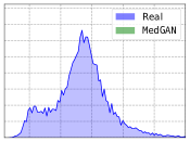
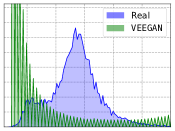
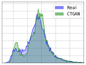
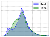
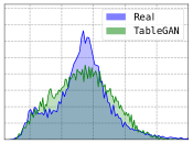
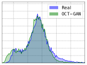
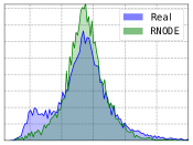
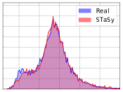
Figure 5: Histograms of values in the excess kurtosis column of HTRU

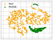
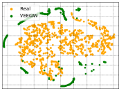
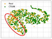
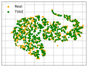
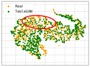
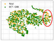
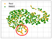
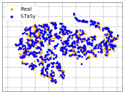
Figure 6: t-SNE visualizations of fake and original records in HTRU

J.2 Additional visualizations in Robot

In Robot, TVAE, OCT-GAN, and STaSy generate relatively similar distribution to that of real data as shown in Figure 7. In Figure 8, CTGAN, TableGAN, and RNODE generate out-of-distribution records as highlighted in red, and TVAE and OCT-GAN suffer from mode collapses. Our proposed methods generate the most diverse records among various methods.

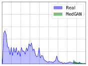
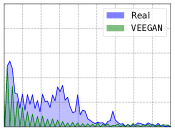
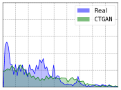
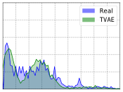
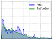
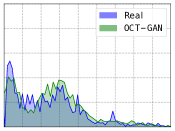
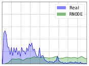
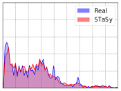
Figure 7: Histograms of values in the ultrasound sensor column of Robot

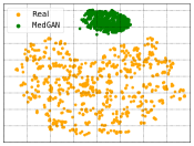
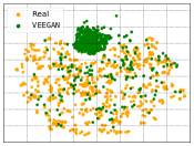
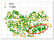
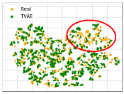
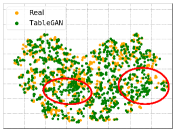
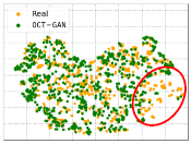
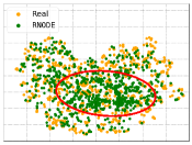
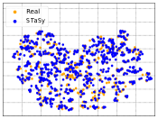
Figure 8: t-SNE visualizations of fake and original records in Robot

J.3 Additional visualizations in News

In News, the fake data by STaSy shows more reliable column-wise histogram than others in Figure 9. As shown in Figure 10, all methods except for TableGAN and RNODE well generate fake records.

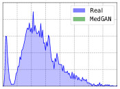
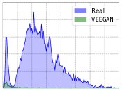
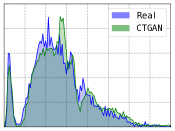
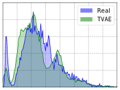
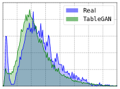
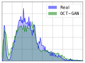
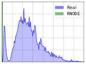
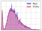
Figure 9: Histograms of values in the min of best keyword column of News

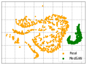
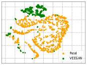
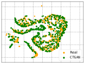
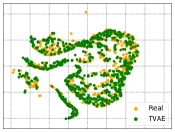
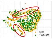
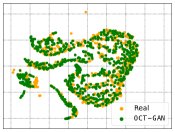
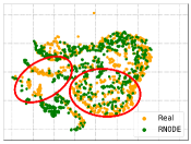
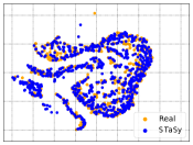
Figure 10: t-SNE visualizations of fake and original records in News

References

- (1) Statlog (Shuttle). UCI Machine Learning Repository.
- Aviñó et al. (2018) Laura Aviñó, Matteo Ruffini, and Ricard Gavaldà. Generating synthetic but plausible healthcare record datasets, 2018.
- Bazaraa et al. (1993) M.S. Bazaraa, H.D. Sherali, and C.M. Shetty. Nonlinear Programming Theory and Algorithms. John Wiley, New York, 1993.
- Bock (2007) R. Bock. MAGIC Gamma Telescope. UCI Machine Learning Repository, 2007.
- Chawla et al. (2002) Nitesh V Chawla, Kevin W Bowyer, Lawrence O Hall, and W Philip Kegelmeyer. Smote: synthetic minority over-sampling technique. Journal of artificial intelligence research, 16:321–357, 2002.
- Che et al. (2017) Zhengping Che, Yu Cheng, Shuangfei Zhai, Zhaonan Sun, and Yan Liu. Boosting deep learning risk prediction with generative adversarial networks for electronic health records. 2017.
- Chen et al. (2018) Tian Chen, Yulia Rubanova, Jesse Bettencourt, and David Duvenaud. Neural ordinary differential equations, 06 2018.
- Choi et al. (2017) Edward Choi, Siddharth Biswal, A. Bradley Maline, Jon Duke, F. Walter Stewart, and Jimeng Sun. Generating multi-label discrete electronic health records using generative adversarial networks. 2017.
- Esteban et al. (2017) Cristóbal Esteban, L. Stephanie Hyland, and Gunnar Rätsch. Real-valued (medical) time series generation with recurrent conditional gans, 2017.
- Fernandes et al. (2015) Kelwin Fernandes, Pedro Vinagre, and Paulo Cortez. A proactive intelligent decision support system for predicting the popularity of online news. In Portuguese conference on artificial intelligence, pp. 535–546. Springer, 2015.
- Finlay et al. (2020) Chris Finlay, Jörn-Henrik Jacobsen, Levon Nurbekyan, and Adam M. Oberman. How to train your neural ode: the world of jacobian and kinetic regularization. In ICML, 2020.
- Freire et al. (2010) Freire, Ananda, Veloso, Marcus, Barreto, and Guilherme. Wall-Following Robot Navigation Data. UCI Machine Learning Repository, 2010.
- Grathwohl et al. (2018) Will Grathwohl, Ricky TQ Chen, Jesse Bettencourt, Ilya Sutskever, and David Duvenaud. Ffjord: Free-form continuous dynamics for scalable reversible generative models. arXiv preprint arXiv:1810.01367, 2018.
- Han et al. (2005) Hui Han, Wen-Yuan Wang, and Bing-Huan Mao. Borderline-smote: A new over-sampling method in imbalanced data sets learning. In Proceedings of the 2005 International Conference on Advances in Intelligent Computing - Volume Part I, ICIC’05, pp. 878–887, Berlin, Heidelberg, 2005. Springer-Verlag. ISBN 3540282262. doi: 10.1007/11538059_91. URL https://doi.org/10.1007/11538059_91.
- He et al. (2008) Haibo He, Yang Bai, Edwardo Garcia, and Shutao Li. Adasyn: Adaptive synthetic sampling approach for imbalanced learning. pp. 1322 – 1328, 07 2008. doi: 10.1109/IJCNN.2008.4633969.
- Hopkins et al. (1999) Hopkins, Mark, Reeber, Erik, Forman, George & Suermondt, and Jaap. Spambase. UCI Machine Learning Repository, 1999.
- Hutchinson (1989) M.F. Hutchinson. A stochastic estimator of the trace of the influence matrix for laplacian smoothing splines. Communication in Statistics- Simulation and Computation, 18:1059–1076, 01 1989. doi: 10.1080/03610919008812866.
- Jiang et al. (2014) Lu Jiang, Deyu Meng, Shoou-I Yu, Zhenzhong Lan, Shiguang Shan, and Alexander Hauptmann. Self-paced learning with diversity. Advances in neural information processing systems, 27, 2014.
- Johnson & Iizuka (2016) Brian A. Johnson and Kotaro Iizuka. Integrating openstreetmap crowdsourced data and landsat time-series imagery for rapid land use/land cover (lulc) mapping: Case study of the laguna de bay area of the philippines. Applied Geography, 67(C):140–149, 2016. doi: 10.1016/j.apgeog.2015.12.006.
- Jordon et al. (2019) James Jordon, Jinsung Yoon, and V. D. Mihaela Schaar. Pate-gan: Generating synthetic data with differential privacy guarantees. In International Conference on Learning Representations, 2019.
- Kim et al. (2021) Jayoung Kim, Jinsung Jeon, Jaehoon Lee, Jihyeon Hyeong, and Noseong Park. Oct-gan: Neural ode-based conditional tabular gans. In TheWebConf, 2021.
- Kim et al. (2022) Jayoung Kim, Chaejeong Lee, Yehjin Shin, Sewon Park, Minjung Kim, Noseong Park, and Jihoon Cho. Sos: Score-based oversampling for tabular data. arXiv preprint arXiv:2206.08555, 2022.
- Koklu & Ozkan (2020) Murat Koklu and Ilker Ali Ozkan. Multiclass classification of dry beans using computer vision and machine learning techniques. Comput. Electron. Agric., 174:105507, 2020.
- Kumar et al. (2010a) M. Kumar, Ben Packer, and Daphne Koller. Self-paced learning for latent variable models. pp. 1189–1197, 01 2010a.
- Kumar et al. (2010b) M Kumar, Benjamin Packer, and Daphne Koller. Self-paced learning for latent variable models. Advances in neural information processing systems, 23, 2010b.
- Lee et al. (2021) Jaehoon Lee, Jihyeon Hyeong, Jinsung Jeon, Noseong Park, and Jihoon Cho. Invertible tabular GANs: Killing two birds with one stone for tabular data synthesis. In NeurIPS, 2021.
- Liang et al. (2015) Xuan Liang, Tao Zou, Bin Guo, Shuo Li, Haozhe Zhang, Shuyi Zhang, Hui Huang, and Song Xi Chen. Assessing beijing’s pm2. 5 pollution: severity, weather impact, apec and winter heating. Proceedings of the Royal Society A: Mathematical, Physical and Engineering Sciences, 471(2182):20150257, 2015.
- Lichman (2013) M. Lichman. UCI machine learning repository, 2013. URL http://archive.ics.uci.edu/ml.
- Lim (1997) Tjen-Sien Lim. Contraceptive Method Choice. UCI Machine Learning Repository, 1997.
- Lyon (2017) Robert Lyon. HTRU2. UCI Machine Learning Repository, 2017.
- Mohammad (2015) Lee Mohammad, Rami & McCluskey. Phishing Websites. UCI Machine Learning Repository, 2015.
- Naeem et al. (2020) Muhammad Ferjad Naeem, Seong Joon Oh, Youngjung Uh, Yunjey Choi, and Jaejun Yoo. Reliable fidelity and diversity metrics for generative models. In International Conference on Machine Learning, pp. 7176–7185. PMLR, 2020.
- Palechor & de la Hoz Manotas (2019) Fabio Mendoza Palechor and Alexis de la Hoz Manotas. Dataset for estimation of obesity levels based on eating habits and physical condition in individuals from colombia, peru and mexico. Data in brief, 25:104344, 2019.
- Park et al. (2018) Noseong Park, Mahmoud Mohammadi, Kshitij Gorde, Sushil Jajodia, Hongkyu Park, and Youngmin Kim. Data synthesis based on generative adversarial networks. arXiv preprint arXiv:1806.03384, 2018.
- Patel et al. (2018) Shreyas Patel, Ashutosh Kakadiya, Maitrey Mehta, Raj Derasari, Rahul Patel, and Ratnik Gandhi. Correlated discrete data generation using adversarial training. 2018.
- Patki et al. (2016) Neha Patki, Roy Wedge, and Kalyan Veeramachaneni. The synthetic data vault. In DSAA, 2016.
- Reiter (2005) P. Jerome Reiter. Using cart to generate partially synthetic, public use microdata. Journal of Official Statistics, 21:441, 01 2005.
- Sakar et al. (2019) C. Okan Sakar, S. Polat, Mete Katircioglu, and Yomi Kastro. Real-time prediction of online shoppers’ purchasing intention using multilayer perceptron and lstm recurrent neural networks. Neural Computing and Applications, 31, 10 2019. doi: 10.1007/s00521-018-3523-0.
- Song et al. (2021) Yang Song, Jascha Sohl-Dickstein, Diederik P Kingma, Abhishek Kumar, Stefano Ermon, and Ben Poole. Score-based generative modeling through stochastic differential equations. In ICLR, 2021.
- Srivastava et al. (2017) Akash Srivastava, Lazar Valkov, Chris Russell, Michael U Gutmann, and Charles Sutton. Veegan: Reducing mode collapse in gans using implicit variational learning. Advances in neural information processing systems, 30, 2017.
- Tang et al. (2012) Kevin Tang, Vignesh Ramanathan, Li Fei-Fei, and Daphne Koller. Shifting weights: Adapting object detectors from image to video. In Proceedings of the 25th International Conference on Neural Information Processing Systems - Volume 1, NIPS’12, pp. 638–646, Red Hook, NY, USA, 2012. Curran Associates Inc.
- van der Maaten & Hinton (2008) Laurens van der Maaten and Geoffrey Hinton. Visualizing data using t-sne. Journal of Machine Learning Research, 9(86), 2008.
- Vincent (2011) Pascal Vincent. A connection between score matching and denoising autoencoders. Neural Comput., 23(7):1661–1674, 2011.
- Xiao et al. (2021) Zhisheng Xiao, Karsten Kreis, and Arash Vahdat. Tackling the generative learning trilemma with denoising diffusion gans, 12 2021.
- Xu et al. (2019) Lei Xu, Maria Skoularidou, Alfredo Cuesta-Infante, and Kalyan Veeramachaneni. Modeling tabular data using conditional gan. In NeurIPS. 2019.
- Zhang et al. (2017) Jun Zhang, Graham Cormode, Cecilia M. Procopiuc, Divesh Srivastava, and Xiaokui Xiao. Privbayes: Private data release via bayesian networks. ACM Transactions on Database Systems, 2017.