Determinantal Coulomb gas ensembles with a class of discrete rotational symmetric potentials

Abstract.

We consider determinantal Coulomb gas ensembles with a class of discrete rotational symmetric potentials whose droplets consist of several disconnected components. Under the insertion of a point charge at the origin, we derive the asymptotic behaviour of the correlation kernels both in the macro- and microscopic scales. In the macroscopic scale, this particularly shows that there are strong correlations among the particles on the boundary of the droplets. In the microscopic scale, this establishes the edge universality. For the proofs, we use the nonlinear steepest descent method on the matrix Riemann-Hilbert problem to derive the asymptotic behaviours of the associated planar orthogonal polynomials and their norms up to the first subleading terms.

1. Introduction and main results

We consider a configuration $\{z_{j}\}_{1}^{N}$ of $N$ points in $\mathbb{C}$ with joint probability distribution

(1.1) $$d\mathbf{P}_{N}=\frac{1}{Z_{N}}\prod_{j>k}|z_{j}-z_{k}|^{2}\prod_{j=1}^{N}e^{-NQ(z_{j})}\,dA(z_{j}),\qquad dA(z):=\frac{d^{2}z}{\pi},$$

where $Z_{N}$ is the normalisation constant and $Q:\mathbb{C}\to\mathbb{R}$ is a suitable function called external potential. The ensemble (1.1) corresponds to the eigenvalue system of the random normal matrix model, which can be interpreted as the two-dimensional Coulomb gas ensemble at a specific inverse temperature $\beta=2$. For a recent account of the theory and various topics on the Coulomb gas ensemble, we refer the reader to [41] and references therein.

By definition, the $k$-point correlation function $R_{N,k}$ of the system (1.1) is given by

(1.2) $$R_{N,k}(z_{1},\cdots,z_{k}):=\frac{N!}{(N-k)!}\int_{\mathbb{C}^{n-k}}\mathbf{P}_{N}\prod_{j=k+1}^{N}dA(z_{j}).$$

The normalised $1$-point function $\frac{1}{N}R_{N,1}$ corresponds to the macroscopic density of the model. It is well known that as $N\to\infty$, the empirical measure of $\{z_{j}\}_{1}^{N}$ converges to Frostman’s equilibrium measure, see e.g. [25, 5]. In particular, the system $\{z_{j}\}_{1}^{N}$ tends to occupy certain compact set $S$ called the droplet.

The $k$-point function $R_{N,k}$ can be effectively analysed in terms of the correlation kernel. To be more concrete, let $p_{k}\equiv p_{k,N}$ be the $k$:th orthonormal polynomial with respect to the weighted Lebesgue measure $e^{-NQ}\,dA$:

(1.3) $$\int_{\mathbb{C}}p_{j}(z)\overline{p_{k}(z)}e^{-NQ(z)}\,dA(z)=\delta_{jk},$$

where $\delta_{jk}$ is the Kronecker delta. We write

(1.4) $$K_{N}(z,w)=e^{-\frac{N}{2}(Q(z)+Q(w))}\sum_{j=0}^{N-1}p_{j}(z)\overline{p_{j}(w)}$$

for the weighted reproducing kernel of analytic polynomials (of degree less than $N-1$) in $L^{2}(e^{-NQ}\,dA)$. Then the $k$-point function $R_{N,k}$ in (1.2) is expressed as

(1.5) $$R_{N,k}(z_{1},\cdots,z_{k})=\det\Big{[}K_{N}(z_{j},z_{l})\Big{]}_{j,l=1}^{k}.$$

We mention that the correlation kernel can be defined up to a sequence of cocycles, i.e.

(1.6) $$\det\Big{[}K_{N}(z_{j},z_{l})\Big{]}_{j,l=1}^{k}=\det\Big{[}g_{N}(z_{j})\,\overline{g_{N}(z_{l})}\cdot K_{N}(z_{j},z_{l})\Big{]}_{j,l=1}^{k},$$

where $g_{N}$ is a continuous unimodular function.

Due to the property (1.5), the system (1.1) is also called the determinantal Coulomb gas ensemble. Moreover, this naturally calls for the investigation of various asymptotic behaviours of $K_{N}$ as $N\to\infty$. Here, one has to distinguish two cases, the macroscopic scale and the microscopic scale.

The asymptotic behaviour in the microscopic scale is closely related to the universality principle in random matrix theory. To describe the local statistics of the model at a given base point $p\in S$, one needs to investigate the asymptotic behaviour of the function

(1.7) $$(z,w)\mapsto K_{N}\Big{(}p+\frac{e^{i\theta}\,z}{\sqrt{N\Delta Q(p)}}\,,p+\frac{e^{i\theta}\,w}{\sqrt{N\Delta Q(p)}}\Big{)}.$$

Here if $p\in\partial S$, the angle $\theta\in[0,2\pi)$ is chosen so that $e^{i\theta}$ is outer normal to $\partial S$ at $p$, and otherwise $\theta=0.$ We remark that the specific choice of the rescaling factor $\sqrt{N\Delta Q(p)}$ in (1.7) (which is often called the “unfolding”) comes from the fact that $\frac{1}{N}R_{N,1}(p)\sim\Delta Q(p)$.

For the bulk case when $p\in\operatorname{Int}S$, it was shown in [8] that for a general external potential $Q$,

(1.8) $$K_{N}\Big{(}p+\frac{z}{\sqrt{N\Delta Q(p)}}\,,p+\frac{w}{\sqrt{N\Delta Q(p)}}\Big{)}\to G(z,w):=e^{z\bar{w}-\frac{|z|^{2}}{2}-\frac{|w|^{2}}{2}}.$$

Here $\operatorname{Int}S$ stands for the interior of $S$, the largest open set of $S$, and the universal scaling limit $G$ in (1.8) is called the Ginibre kernel [32]. For the edge case when $p\in\partial S$, it was shown in a fairly recent work [35] that for a general external potential $Q$,

(1.9) $$K_{N}\Big{(}p+\frac{e^{i\theta}\,z}{\sqrt{N\Delta Q(p)}}\,,p+\frac{e^{i\theta}\,w}{\sqrt{N\Delta Q(p)}}\Big{)}\to G(z,w)\,\frac{1}{2}\operatorname{erfc}\Big{(}\frac{z+\bar{w}}{\sqrt{2}}\Big{)}.$$

The class of potentials $Q$ covered in [35] is quite general but dependent on the topology of the associated droplet.

Turning to the macroscopic scale, recently, Ameur and Cronvall [7] made significant results on the asymptotic behaviour of $K_{N}(z,w)$. For the Ginibre ensemble with $Q(z)=|z|^{2}$, they obtained a precise asymptotic result. Namely, it was obtained in [7, Theorem 1.1] that

(1.10) $$K_{N}(z,w)=\sqrt{\frac{N}{2\pi}}\frac{1}{z\bar{w}-1}(z\bar{w})^{N}e^{N-\frac{N}{2}(|z|^{2}+|w|^{2})}\cdot\Big{(}1+O(\frac{1}{N})\Big{)},$$

where $z\not=w$ and $z\bar{w}$ is outside the Szegő curve

(1.11) $$\mathcal{S}_{1}:=\{z\in\mathbb{C}:|z|\leq 1,|z\,e^{1-z}|=1\}.$$

Here, we intentionally add the subscript $1$ since (1.11) can be realised as a special case of $\SS_{a}$ in (1.13) below with $a=1$. We stress that [7, Theorem 1.1] indeed provides a closed form of large-$N$ expansions of $K_{N}.$ Let us also mention that (1.10) can also be interpreted as an asymptotic result of the incomplete gamma function with complex argument, see [7, Section 1.4] and (A.6). (Cf. this was crucially used in a recent work [20].)

Beyond the Ginibre ensemble, Ameur and Cronvall considered general external potential $Q$ and derived the uniform asymptotic behaviour of $K_{N}(z,w)$ for $z,w$ outside the droplet, see [7, Theorem 1.3]. (We also refer to [3, 31, 42] for similar results on the elliptic Ginibre ensemble.) In particular, they showed that there are strong correlations among the particles on the boundary of the droplet. One of the main ingredients in their proof is the asymptotic behaviour of planar orthogonal polynomials (1.3) due to Hedenmalm and Wennman [35].

The above-mentioned results were mainly obtained for the case where the external potential $Q$ is fixed, i.e. independent of $N$. Nevertheless, the case when $Q$ depends on $N$ is also interesting in particular in the context of the insertion of point charges [11] also known as the induced ensembles [30] or spectral singularities [36]. (Another important example that $N$-dependence of the potential being crucial is the almost-Hermitian regime, see e.g. [6].)

Furthermore, in [35] (and also in the follow-up paper [34]), the asymptotic behaviours of planar orthogonal polynomials were constructed in terms of a conformal map from the outside the droplet onto the outside the unit disc. Accordingly, the asymptotic result in [35] was obtained for the potential $Q$ whose associated droplet is simply connected as a domain on the Riemann sphere. As a consequence, the edge universality (1.9) in [35] as well as the Szegő type asymptotic behaviour in [7] were obtained under the assumption that the associated droplet does not have several disconnected components.

In this work, we aim to provide concrete examples of asymptotic results for the ensembles with a class of $N$-dependent potentials associated with disconnected droplets, see Figure 1.

Figure 1. Illustration of the lemniscate archipelago and zooming process

1.1. Main results

We now precisely introduce our models. It is more convenient to begin with a special case when removing the discrete rotational symmetry. In this case, the model corresponds to the induced Ginibre ensemble [30] with the potential

(1.12) $$Q_{c}(z)\equiv Q_{N,c}(z):=|z|^{2}-\frac{2c}{N}\log|z-a|,$$

where $c>-1$ and $a\geq 0$. From the statistical physics point of view, we insert a point charge $c$ at a given point $a$. When $c$ is an integer, the ensemble (1.1) with the potential (1.12) can also be realised as the Ginibre ensemble conditioned to have eigenvalue $a$ with multiplicity $c$.

The orthogonal polynomials associated with (1.12) reveal a discontinuity at $c=0$. Namely, if $c=0$, since the orthogonal polynomials are simply given by monomials, all the zeros are located at the origin. On the other hand, in [38], it was shown that for any $c\not=0$ and $a>1$, the zeros of orthogonal polynomials tend to occupy the limiting skeleton (also known as mother body, cf. [33])

(1.13) $$\mathcal{S}_{a}:=\Big{\{}z\in\mathbb{C}:\log|z|-a\operatorname{Re}z=\log\Big{(}\frac{1}{a}\Big{)}-1\,,\,\operatorname{Re}z\leq\frac{1}{a}\Big{\}}.$$

Note that $\SS_{a}$ crosses the point $1/a$. The limiting skeleton $\SS_{a}$ plays an important role in the asymptotic behaviours of the orthogonal polynomials. See Figure 2 for the shape of $\SS_{a}$.

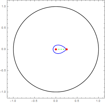
(a) $a=4$

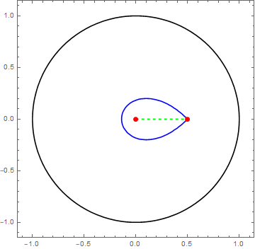
(b) $a=2$

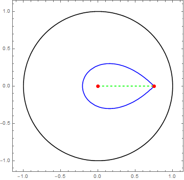
(c) $a=4/3$

Figure 2. The plots display $\SS_{a}$. The red dots show the origin and $1/a$. The green dashed lines indicate the branch cuts in Theorem 1.1.

In our first result, we obtain the following asymptotic behaviour of $K_{N}$ in the macroscopic scaling.

Theorem 1.1.

(Macroscopic asymptotic of the induced Ginibre ensemble) Let $Q$ be the induced Ginibre potential (1.12) with $a>1$ and $c>-1$ $(c\not=0)$. Suppose that $z$ and $w$ are outside $\SS_{a}$, and $|z-w|>\delta$ for some $\delta>0$. Then we have

(1.14) $$K_{N}(z,w)=\sqrt{\frac{N}{2\pi}}\frac{1}{z\bar{w}-1}\,\Big{(}\frac{z}{1-az}\frac{\bar{w}}{1-a\bar{w}}\Big{)}^{c}(z\bar{w})^{N}|(z-a)(w-a)|^{c}e^{N-\frac{N}{2}(|z|^{2}+|w|^{2})}\cdot\Big{(}1+O(\frac{1}{N})\Big{)}.$$

Here the branch cuts for the variables $z$ and $\bar{w}$ are the line segment $[0,1/a]$.

Note that if we formally put $c=0$, the formula (1.14) corresponds (1.10). We mention that the condition $z$ and $w$ being outside the limiting skeleton was also considered in [3] for the elliptic Ginibre ensemble. (In this case, the limiting skeleton is a line segment connecting two foci of the ellipse.)

In the spirit of the edge universality (1.9), we obtain the following.

Theorem 1.2.

(Boundary scaling limits of the induced Ginibre ensemble) Let $Q$ be the induced Ginibre potential (1.12) with $a>1$ and $c>-1$. Let $p$ be a point on the unit circle. Then as $N\to\infty$, we have

(1.15) $$\frac{1}{N}K_{N}\Big{(}p+\frac{p\,z}{\sqrt{N}}\,,\,p+\frac{p\,w}{\sqrt{N}}\Big{)}\to G(z,w)\,\frac{1}{2}\operatorname{erfc}\Big{(}\frac{z+\bar{w}}{\sqrt{2}}\Big{)},$$

uniformly for $z,w$ on compact subsets of $\mathbb{C}$.

We now discuss the ensemble with discrete rotational symmetry. For $a\geq 0$ and $d\in\mathbb{N}$, let

(1.16) $$V(z)=\frac{1}{d}|z^{d}-a|^{2},\qquad V_{c}(z)\equiv V_{N,c}:=V(z)-\frac{2c}{N}\log|z|.$$

We refer to [10, 21, 27] and references therein for recent studies on such models. Note that the induced Ginibre potential (1.12) corresponds to (1.16) with $d=1$ up to a translation. It is well known that the droplet $S_{V}$ associated with the potential $V$ is given by

(1.17) $$S_{V}:=\{z\in\mathbb{C}:|z^{d}-a|\leq 1\},$$

see e.g. [14, Lemma 1]. The density with respect to $dA$ is given by

(1.18) $$\Delta V(z)=d\,|z|^{2d-2}.$$

Due to the explicit formula (1.17), one can easily notice that if $a<1$, $S_{V}$ is connected. On the other hand, if $a>1$, $S_{V}$ consists of $d$-connected components that we call the lemniscate archipelago following [7], see Figure 1.

We denote by $q_{j,N}^{c}$ the orthonormal polynomials associated with the weighted measure $e^{-NV_{c}}\,dA$:

(1.19) $$\int_{\mathbb{C}}q_{j,N}^{c}(z)\overline{q_{k,N}^{c}(z)}|z|^{2c}e^{-NV(z)}\,dA(z)=\delta_{jk}.$$

For $a>1$, it was shown in [13, 38] that as $j\to\infty$, the (non-trivial) zeros of $q_{j,N}^{c}$ tend to accumulate on the curve

(1.20) $$\mathcal{S}_{a}^{d}:=\Big{\{}z\in\mathbb{C}:\log|z^{d}-a|+a\operatorname{Re}z^{d}=\log\Big{(}\frac{1}{a}\Big{)}-1+a^{2}\,,\,\operatorname{Re}z^{d}\geq a-\frac{1}{a}\Big{\}}.$$

Notice that (1.20) and (1.13) are related by the mapping $z\mapsto a-z^{d}$. See Figure 3 for the shape of $\SS_{a}^{d}$.

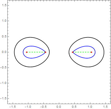
(a) $d=2$

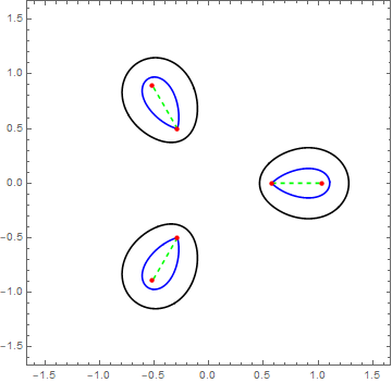
(b) $d=3$

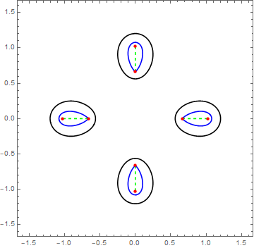
(c) $d=4$

Figure 3. The plots display $\partial S_{V}$ (black) and $\mathcal{S}_{a}^{d}$ (blue), where $a=1.1$. The red dots indicate $(a-\frac{1}{a})^{1/d}\omega^{k}$ and $a^{1/d}\omega^{k}$. The green dashed lines are the branch cuts in (1.22).

Let us consider the associated correlation kernel

(1.21) $$K_{N}^{c}(z,w):=|zw|^{c}e^{-\frac{N}{2}(V(z)+V(w))}\sum_{j=0}^{N-1}q_{j,N}^{c}(z)\overline{q_{j,N}^{c}(w)}.$$

The kernel (1.21) corresponds to the reproducing kernel (1.4) associated with the potential $Q=V_{c}.$ We derive the asymptotic behaviours of $K_{N}^{c}$ in the macroscopic scale.

Theorem 1.3.

(Macroscopic asymptotic of the lemniscate archipelago) Let $d>1$, $a>1$ and $c>-1$ be fixed. Suppose that $z$ and $w$ are outside $\SS_{a}^{d}$, and $|z-w|>\delta$ for some $\delta>0$. If $c=0,1,\dots,d-1$, we further assume that $(z^{d}-a)(\bar{w}^{d}-a)$ is outside $\SS_{1}$. Then as $N\to\infty,$ we have

(1.22) $$\begin{split}K_{dN}^{c}(z,w)&=d\sqrt{\frac{N}{2\pi}}\frac{((z^{d}-a)(\bar{w}^{d}-a))^{N}}{(z^{d}-a)(\bar{w}^{d}-a)-1}\,|z\bar{w}|^{c}e^{N-\frac{dN}{2}(V(z)+V(w))}\\ &\quad\times\Big{(}\frac{z^{d}-a}{az^{d}+1-a^{2}}\frac{\bar{w}^{d}-a}{a\bar{w}^{d}+1-a^{2}}\Big{)}^{\frac{c}{d}}((z^{d}-a)(\bar{w}^{d}-a))^{\frac{1}{d}-1}\\ &\quad\times\frac{(az^{d}+1-a^{2})(a\bar{w}^{d}+1-a^{2})-z^{d}(z^{d}-a)\bar{w}^{d}(\bar{w}^{d}-a)}{(az^{d}+1-a^{2})^{\frac{1}{d}}(a\bar{w}^{d}+1-a^{2})^{\frac{1}{d}}-z(z^{d}-a)^{\frac{1}{d}}\bar{w}(\bar{w}^{d}-1)^{\frac{1}{d}}}\cdot\Big{(}1+O(\frac{1}{N})\Big{)}.\end{split}$$

Here the branch cuts for the variables $z$ and $\bar{w}$ are given by the combination of $d$ line segments connecting $(a-\frac{1}{a})^{1/d}\omega^{k}$ and $a^{1/d}\omega^{k}$, where $\omega=e^{2\pi i/d}$ and $k=0,1,\dots,d-1.$

Note that by (1.16) and (1.17), we have

(1.23) $$|z^{d}-a|=1,\qquad V(z)=\frac{1}{d},\qquad(z\in\partial S_{V}).$$

Then as an immediate consequence of Theorem 1.3, we obtain that for $z,w\in\partial S_{V}$,

(1.24) $$\begin{split}|K_{dN}^{c}(z,w)|&=d\sqrt{\frac{N}{2\pi}}\Big{|}\frac{(z\bar{w})^{c}}{(z^{d}-a)(\bar{w}^{d}-a)-1}\Big{(}(az^{d}+1-a^{2})(a\bar{w}^{d}+1-a^{2})\Big{)}^{-\frac{c}{d}}\Big{|}\\ &\quad\times\Big{|}\frac{(az^{d}+1-a^{2})(a\bar{w}^{d}+1-a^{2})-z^{d}(z^{d}-a)\bar{w}^{d}(\bar{w}^{d}-a)}{(az^{d}+1-a^{2})^{\frac{1}{d}}(a\bar{w}^{d}+1-a^{2})^{\frac{1}{d}}-z(z^{d}-a)^{\frac{1}{d}}\bar{w}(\bar{w}^{d}-1)^{\frac{1}{d}}}\Big{|}\cdot\Big{(}1+O(\frac{1}{N})\Big{)}.\end{split}$$

Thus one can notice that $K_{dN}^{c}(z,w)=O(\sqrt{N})$ for $z,w\in\partial S_{V}$, which indicates that there are strong correlations among the particles on the boundary of the droplets.

To provide a physical realisation of Theorem 1.3, let us consider the Berezin kernel

(1.25) $$B_{N}(z,w):=\frac{R_{N,1}(z)R_{N,1}(w)-R_{N,2}(z,w)}{R_{N,1}(z)}=\frac{|K_{N}^{c}(z,w)|^{2}}{R_{N,1}(z)}.$$

For a given point $z$, the function $w\mapsto B_{N}(z,w)$ corresponds to the probability density of the ensemble conditioned to have a particle at $z.$ See Figure 4 for the graphs of $B_{N}$.

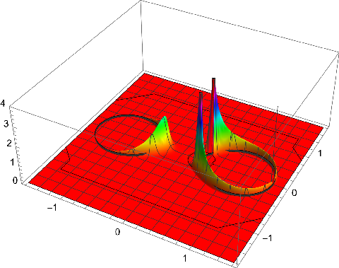
(a) $d=2$

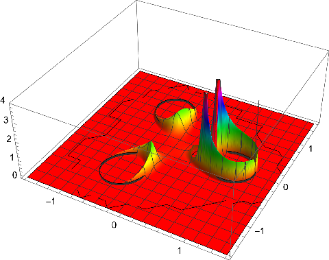
(b) $d=3$

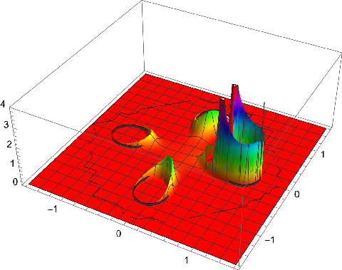
(c) $d=4$

Figure 4. The plots display the approximation of the graphs $w\mapsto B_{N}(z,w)$ in (1.25) (for $w$ away from $z$), where $z=(a-1)^{\frac{1}{d}}\in\partial S_{V}$ and $a=1.1$. Here $c=0$ and $N=600$. For the approximation, we use (1.22) and the fact that $R_{N,1}(z)\sim N\Delta V(z)/2$.

We remark that the asymptotic behaviour (1.22) may involve special functions (in the subleading terms) with certain periodicity such as Jacobi theta functions as observed in [26] for a rotationally symmetric ensemble. We refer to [28, 18] for a discussion on similar situations on Hermitian matrix model.

In our final result, we derive the boundary scaling limits.

Theorem 1.4.

(Boundary scaling limits of the lemniscate archipelago) Let $p\in\partial S_{V}$ and choose $\theta$ so that $e^{i\theta}$ is outer normal to $\partial S_{V}$ at $p$. Then as $N\to\infty$, we have

(1.26) $$\frac{1}{dN\Delta V(p)}K_{dN}^{c}\Big{(}p+\frac{e^{i\theta}\,z}{\sqrt{dN\Delta V(p)}}\,,\,p+\frac{e^{i\theta}\,w}{\sqrt{dN\Delta V(p)}}\Big{)}\to G(z,w)\,\frac{1}{2}\operatorname{erfc}\Big{(}\frac{z+\bar{w}}{\sqrt{2}}\Big{)},$$

uniformly for $z,w$ on compact subsets of $\mathbb{C}$.

We emphasise that Theorem 1.4 provides an example of edge universality for the ensembles with disconnected droplets that are not covered in [35].

1.2. Outline of the proofs

The overall strategy of the proofs is as follows.

• We use the multi-fold transform of the correlation kernels (Lemma 2.1) that relates those of $Q_{c}$ in (1.12) and of $V_{c}$ in (1.16). Due to this property, one can easily derive Theorems 1.3 and  1.4 from Theorems 1.1 and  1.2, respectively.

• We apply the generalised Christoffel-Darboux formula (Proposition 2.2) that allows expressing the correlation kernel only in terms of three monic orthogonal polynomials (of degree $N-1$, $N$, and $N+1$) and their norms.

• Using the steepest descent method to the Riemann-Hilbert problem developed in [12, 38], we derive the asymptotic behaviours of orthogonal polynomials (Proposition 2.3) and norms (Lemma 2.4) up to the first subleading terms. Combined with the Christoffel-Darboux formula, these lead to Theorems 1.1 and  1.2.

The overall strategy described above was introduced in [24] to obtain the microscopic limit of the correlation kernel at multi-criticality $a=1$. We use this strategy when $a>1$ together with new asymptotic behaviours of orthogonal polynomials and their norms (Proposition 2.3 and Lemma 2.4). These are probably of interest by themselves in the spirit of several works [13, 40, 15, 19] on Riemann-Hilbert analysis for planar orthogonal polynomials.

The rest of this paper is organised as follows. In Section 2, we present the overall strategy of the proofs in more detail and show our main results. However it requires Proposition 2.3 and Lemma 2.4 that are only shown in the following section. For the proofs, in Section 3, we use the nonlinear steepest descent method to the Riemann-Hilbert problem associated with the orthogonal polynomials. In Appendix A, we present the proofs of Proposition 2.3 and Lemma 2.4 for the exactly solvable case $c=1$ using well-known properties of some special functions.

2. Proofs of main results

In this section, we present the overall strategy of the proofs and show the main results. In Subsections 2.1 and  2.2 we introduce the multi-fold transform (Lemma 2.1) and the generalised Christoffel-Darboux formula. In Subsection 2.3, we present asymptotic behaviours of orthogonal polynomials (Proposition 2.3) and the norms (Lemma 2.4). In Subsection 2.4, we prove Theorems 1.1 and  1.2. In the last subsection, we show Theorems 1.3 and  1.4.

2.1. Multi-fold transform

We write $p_{j,N}^{c}$ for the orthonormal polynomials satisfying

(2.1) $$\int_{\mathbb{C}}p_{j,N}^{c}(z)\overline{p_{k,N}^{c}(z)}|z|^{2c}e^{-N|z-a|^{2}}\,dA(z)=\delta_{jk}.$$

Then the orthogonal polynomials $q_{j,N}^{c}$ in (1.19) is related to $p_{j,N}^{c}$ as

(2.2) $$q_{dj+l,dN}^{c}(z)=\sqrt{d}\,z^{l}p_{j,N}^{\frac{c+l+1}{d}-1}(z^{d}),$$

see e.g. [15, Section 3] and [24, Section 2]. We now define the correlation kernel

(2.3) $$\widehat{K}_{N}^{c}(z,w)=(z\bar{w})^{c}e^{-\frac{N}{2}(|z-a|^{2}+|w-a|)^{2}}\sum_{j=0}^{N-1}p_{j,N}^{c}(z)\overline{p_{j,N}^{c}(w)}.$$

Notice that we use $(z\bar{w})^{c}$ instead of $|zw|^{c}$.

By (2.2), we have the following multi-fold transform relation, see [24, Section 2] for more detail. (Cf. this idea appeared also in [29, Proposition 2.1], see [1] for the chiral setup.) Recall that $K_{N}^{c}$ is given by (1.21).

Lemma 2.1.

We have

(2.4) $$K_{dN}^{c}(z,w)=d(z\bar{w})^{d-1}\Big{(}\frac{|zw|}{z\bar{w}}\Big{)}^{c}\sum_{l=0}^{d-1}\widehat{K}_{N}^{\frac{c+l+1}{d}-1}(z^{d},w^{d}).$$

Note that in the left-hand side of (2.4) we use $dN$ instead of $N$. This is indeed the key observation for such a transform. Due to Lemma 2.1, it suffices to derive the asymptotics of $\widehat{K}_{N}^{c}$.

2.2. Christoffel-Darboux formula

One can compute asymptotics of $\bar{\partial}_{w}\widehat{K}_{N}^{c}(z,w)$ by virtue of the Christoffel-Darboux formula in [24, Theorem 3.2].

For this, we set some notations. Let $P_{j}\equiv P_{j}^{c}$ be the monic orthogonal polynomial satisfying

(2.5) $$\int_{\mathbb{C}}P_{j}(z)\overline{P_{k}(z)}|z-a|^{2c}e^{-N|z|^{2}}\,dA(z)=h_{j}\,\delta_{jk},$$

where $h_{j}$ is the (squared) orthogonal norm. Note that we have the following relation

(2.6) $$p_{j,N}^{c}(z)=\frac{1}{\sqrt{h_{j}}}P_{j}(a-z).$$

We denote

(2.7) $$W(z)=(z-a)^{c},\qquad\psi_{j}(z):=W(z)P_{j}(z),\qquad\phi_{j}(z):=W(z)\frac{P_{j}(z)}{h_{j}}.$$

Let us define

(2.8) $$\widetilde{K}_{N}^{c}(z,w):=((z-a)(\bar{w}-a))^{c}e^{-Nz\bar{w}}\sum_{j=0}^{N-1}\frac{P_{j}(z)\overline{P_{j}(w)}}{h_{j}}=e^{-Nz\bar{w}}\sum_{j=0}^{N-1}\overline{\phi_{j}(w)}\psi_{j}(z).$$

The kernel $K_{N}$ in (1.4) with $Q$ given by (1.12) is written in terms of $\widetilde{K}_{N}^{c}$ as

(2.9) $$K_{N}(z,w)=\Big{(}\frac{|(z-a)(\bar{w}-a)|}{(z-a)(\bar{w}-a)}\Big{)}^{c}e^{-\frac{N}{2}(|z|^{2}+|w|^{2}-2z\bar{w})}\widetilde{K}_{N}^{c}(z,w).$$

Note also that

(2.10) $$\widetilde{K}_{N}^{c}(a-z,a-w)=(z\bar{w})^{c}e^{-N(a-z)(a-\bar{w})}\sum_{j=0}^{N-1}p_{j,N}^{c}(z)\overline{p_{j,N}^{c}(w)}$$

Thus it is related to $\widehat{K}_{N}^{c}$ in (2.3) as

(2.11) $$\widehat{K}_{N}^{c}(z,w)=e^{-\frac{N}{2}(|z-a|^{2}+|w-a|^{2}-2(z-a)(\bar{w}-a))}\widetilde{K}_{N}^{c}(a-z,a-w).$$

The following version of the Christoffel-Darboux formula was obtained in [24, Theorem 3.2].

Proposition 2.2.

(Christoffel-Darboux formula) Suppose that $a\not=0$ and that

(2.12) $$\langle z\psi_{j}|\phi_{0}\rangle\neq 0,\qquad\phi_{j}(a)\neq 0,\qquad\text{for all }j.$$

Then we have the following form of the Christoffel-Darboux identity:

(2.13) $$\begin{split}{\bar{\partial}}_{w}\widetilde{K}_{N}^{c}(z,w)&=e^{-Nz\bar{w}}\frac{1}{\tfrac{N+c}{N}h_{N-1}-h_{N}}{\bar{\partial}}_{w}\overline{\psi_{N}(w)}\Big{(}\psi_{N}(z)-z\psi_{N-1}(z)\Big{)}\\ &\quad-e^{-Nz\bar{w}}\frac{P_{N+1}(a)}{P_{N}(a)}\frac{N\,h_{N}/h_{N-1}}{\tfrac{N+c+1}{N}h_{N}-h_{N+1}}\overline{\psi_{N-1}(w)}\Big{(}\psi_{N+1}(z)-z\psi_{N}(z)\Big{)}.\end{split}$$

This formula plays a key role in performing asymptotic analysis for Theorems 1.1 and  1.2. We also refer to [37, 2, 16, 22, 20, 23] for various Christoffel-Darboux type identities involving certain differential operators.

2.3. Fine asymptotic behaviours of orthogonal polynomials and norms

Recall that the monic polynomial $P_{j}$ satisfies the orthogonality condition (2.5). The weighted orthogonal polynomial $\psi_{j}$ is given by (2.7). We obtain the strong asymptotic behaviour of $\psi_{j}$ up to the first subleading terms.

Proposition 2.3.

Let $a>1$ and $c>-1$. Then for $z\in\mathbb{C}$ outside $\mathcal{S}_{a}$ in (1.13), we have

(2.14) $$\psi_{N-1}(z) =z^{N+c-1}\Big{(}\frac{z-a}{z-\frac{1}{a}}\Big{)}^{c}\cdot\Big{[}1-\frac{c}{1-az}\Big{(}\frac{1+c}{2}\frac{1}{1-az}+\frac{c}{1-a^{2}}-1\Big{)}\frac{1}{N}+O(\frac{1}{N^{2}})\Big{]},$$

(2.15) $$\psi_{N}(z) =z^{N+c}\Big{(}\frac{z-a}{z-\frac{1}{a}}\Big{)}^{c}\cdot\Big{[}1-\frac{c}{1-az}\Big{(}\frac{1+c}{2}\frac{1}{1-az}+\frac{c}{1-a^{2}}\Big{)}\frac{1}{N}+O(\frac{1}{N^{2}})\Big{]},$$

(2.16) $$\psi_{N+1}(z) =z^{N+c+1}\Big{(}\frac{z-a}{z-\frac{1}{a}}\Big{)}^{c}\cdot\Big{[}1-\frac{c}{1-az}\Big{(}\frac{1+c}{2}\frac{1}{1-az}+\frac{c}{1-a^{2}}+1\Big{)}\frac{1}{N}+O(\frac{1}{N^{2}})\Big{]}.$$

In particular, we have

(2.17) $$\psi_{N}(z)-z\psi_{N-1}(z) =z^{N+c}\Big{(}\frac{z-a}{z-\frac{1}{a}}\Big{)}^{c}\cdot\frac{c}{az-1}\frac{1}{N}\cdot\Big{(}1+O(\frac{1}{N})\Big{)},$$

(2.18) $$\psi_{N+1}(z)-z\psi_{N}(z) =z^{N+1+c}\Big{(}\frac{z-a}{z-\frac{1}{a}}\Big{)}^{c}\cdot\frac{c}{az-1}\frac{1}{N}\cdot\Big{(}1+O(\frac{1}{N})\Big{)}.$$

We emphasise that the leading terms in Proposition 2.3 were obtained in [38, Theorem 2]. Note that the terms (2.17) and (2.18) appear in the Christoffel-Darboux formula (2.13). For these terms, we should extend [38, Theorem 2] up to the first subleading $O(1/N)$ terms.

Notice that if $c=0$, then $\psi_{j}(z)=z^{j}.$ Thus in this case Proposition 2.3 trivially holds.

To apply the Christoffel-Darboux formula (2.13), one should also derive the asymptotic behaviours of the orthogonal norms $h_{j}$ in (2.5).

Lemma 2.4.

Let $a>1$ and $c>-1$. Then we have

(2.19) $$h_{N-1} =e^{-N}\sqrt{\frac{2\pi}{N}}a^{2c}\cdot\Big{[}1+\Big{(}\frac{c}{a^{2}-1}+\frac{c(c-1)}{2}+\frac{1}{12}\Big{)}\frac{1}{N}+O(\frac{1}{N^{2}})\Big{]},$$

(2.20) $$h_{N} =e^{-N}\sqrt{\frac{2\pi}{N}}a^{2c}\cdot\Big{[}1+\Big{(}\frac{c}{a^{2}-1}+\frac{c(c-1)}{2}+\frac{1}{12}\Big{)}\frac{1}{N}+O(\frac{1}{N^{2}})\Big{]},$$

(2.21) $$h_{N+1} =e^{-N}\sqrt{\frac{2\pi}{N}}a^{2c}\cdot\Big{[}1+\Big{(}\frac{c}{a^{2}-1}+\frac{c(c-1)}{2}+\frac{13}{12}\Big{)}\frac{1}{N}+O(\frac{1}{N^{2}})\Big{]}.$$

In particular, for $c\not=0$, we have

(2.22) $$\frac{1}{\tfrac{N+c}{N}h_{N-1}-h_{N}} =\frac{1}{c}\frac{1}{a^{2c}}\frac{1}{\sqrt{2\pi}}\,N^{\frac{3}{2}}\,e^{N}\cdot\Big{(}1+O(\frac{1}{N})\Big{)},$$

(2.23) $$\frac{N\,h_{N}/h_{N-1}}{\tfrac{N+c+1}{N}h_{N}-h_{N+1}} =\frac{1}{c}\frac{1}{a^{2c}}\frac{1}{\sqrt{2\pi}}\,N^{\frac{5}{2}}\,e^{N}\cdot\Big{(}1+O(\frac{1}{N})\Big{)}.$$

Note that (2.22) and (2.23) appear in the Christoffel-Darboux formula (2.13). We remark that for $c=0$, we have

$$h_{j}=\int_{\mathbb{C}}|z|^{2j}e^{-N|z|^{2}}\,dA(z)=2\int_{0}^{\infty}r^{2j+1}e^{-Nr^{2}}\,dr=\frac{j!}{N^{j+1}}.$$

Thus by Stirling’s formula, one can directly check that Lemma 2.4 holds for $c=0.$

2.4. Proofs of Theorems 1.1 and  1.2

Combining the Christoffel-Darboux formula (Proposition 2.2) with Proposition 2.3 and Lemma 2.4, we show Theorem 1.1.

Proof of Theorem 1.1.

By the transform (2.9), it suffices to show that for $z$ and $\bar{w}$ outside $\SS_{a}$ in (1.13),

(2.24) $$\widetilde{K}_{N}^{c}(z,w)=\sqrt{\frac{N}{2\pi}}\frac{1}{z\bar{w}-1}\,\Big{(}\frac{z-a}{1-az}\frac{\bar{w}-a}{1-a\bar{w}}\Big{)}^{c}\cdot(z\bar{w})^{N+c}e^{N-Nz\bar{w}}\cdot\Big{(}1+O(\frac{1}{N})\Big{)}.$$

Using Proposition 2.3, we have

(2.25) $${\bar{\partial}}_{w}\overline{\psi_{N}(w)}=N\bar{w}^{N+c-1}\Big{(}\frac{\bar{w}-a}{\bar{w}-\frac{1}{a}}\Big{)}^{c}\cdot\Big{(}1+O(\frac{1}{N})\Big{)},\qquad\overline{\psi_{N-1}(w)}=\bar{w}^{N+c-1}\Big{(}\frac{\bar{w}-a}{\bar{w}-\frac{1}{a}}\Big{)}^{c}\cdot\Big{(}1+O(\frac{1}{N})\Big{)}.$$

By [38, Theorem 2], we also have

(2.26) $$\frac{P_{N+1}(a)}{P_{N}(a)}=a\cdot\Big{(}1+O(\frac{1}{N})\Big{)}.$$

Therefore by (2.17) and (2.18), we obtain

(2.27) $${\bar{\partial}}_{w}\overline{\psi_{N}(w)}\Big{(}\psi_{N}(z)-z\psi_{N-1}(z)\Big{)}=\frac{c}{az-1}z^{N+c}\bar{w}^{N+c-1}\Big{(}\frac{z-a}{z-\frac{1}{a}}\Big{)}^{c}\Big{(}\frac{\bar{w}-a}{\bar{w}-\frac{1}{a}}\Big{)}^{c}\cdot\Big{(}1+O(\frac{1}{N})\Big{)}$$

and

(2.28) $$\begin{split}\overline{\psi_{N-1}(w)}\Big{(}\psi_{N+1}(z)-z\psi_{N}(z)\Big{)}=\frac{c}{az-1}\frac{1}{N}z^{N+1+c}\bar{w}^{N+c-1}\Big{(}\frac{z-a}{z-\frac{1}{a}}\Big{)}^{c}\Big{(}\frac{\bar{w}-a}{\bar{w}-\frac{1}{a}}\Big{)}^{c}\cdot\Big{(}1+O(\frac{1}{N})\Big{)}.\end{split}$$

Then by Lemma 2.4, we have

(2.29) $$\begin{split}&\quad\frac{1}{\tfrac{N+c}{N}h_{N-1}-h_{N}}{\bar{\partial}}_{w}\overline{\psi_{N}(w)}\Big{(}\psi_{N}(z)-z\psi_{N-1}(z)\Big{)}\\ &=\frac{1}{c}\frac{1}{a^{2c}}\frac{1}{\sqrt{2\pi}}\,N^{\frac{3}{2}}\,e^{N}\frac{c}{az-1}z^{N+c}\bar{w}^{N+c-1}\Big{(}\frac{z-a}{z-\frac{1}{a}}\Big{)}^{c}\Big{(}\frac{\bar{w}-a}{\bar{w}-\frac{1}{a}}\Big{)}^{c}\cdot\Big{(}1+O(\frac{1}{N})\Big{)}\\ &=\frac{1}{\sqrt{2\pi}}\,N^{\frac{3}{2}}\,e^{N}\frac{1}{az-1}z^{N+c}\bar{w}^{N+c-1}\Big{(}\frac{z-a}{1-az}\frac{\bar{w}-a}{1-a\bar{w}}\Big{)}^{c}\cdot\Big{(}1+O(\frac{1}{N})\Big{)}\end{split}$$

and

(2.30) $$\begin{split}&\quad\frac{P_{N+1}(a)}{P_{N}(a)}\frac{N\,h_{N}/h_{N-1}}{\tfrac{N+c+1}{N}h_{N}-h_{N+1}}\overline{\psi_{N-1}(w)}\Big{(}\psi_{N+1}(z)-z\psi_{N}(z)\Big{)}\\ &=a\,\frac{1}{c}\frac{1}{a^{2c}}\frac{1}{\sqrt{2\pi}}\,N^{\frac{5}{2}}\,e^{N}\frac{c}{az-1}\frac{1}{N}z^{N+1+c}\bar{w}^{N+c-1}\Big{(}\frac{z-a}{z-\frac{1}{a}}\Big{)}^{c}\Big{(}\frac{\bar{w}-a}{\bar{w}-\frac{1}{a}}\Big{)}^{c}\cdot\Big{(}1+O(\frac{1}{N})\Big{)}\\ &=\frac{1}{\sqrt{2\pi}}\,N^{\frac{3}{2}}\,e^{N}\frac{az}{az-1}z^{N+c}\bar{w}^{N+c-1}\Big{(}\frac{z-a}{1-az}\frac{\bar{w}-a}{1-a\bar{w}}\Big{)}^{c}\cdot\Big{(}1+O(\frac{1}{N})\Big{)}.\end{split}$$

Now it follows from the Christoffel-Darboux formula (Proposition 2.2) that

(2.31) $${\bar{\partial}}_{w}\widetilde{K}_{N}^{c}(z,w)=-\frac{N^{\frac{3}{2}}}{\sqrt{2\pi}}\,\Big{(}\frac{z-a}{1-az}\frac{\bar{w}-a}{1-a\bar{w}}\Big{)}^{c}\cdot z^{N+c}\bar{w}^{N+c-1}e^{N-Nz\bar{w}}\cdot\Big{(}1+O(\frac{1}{N})\Big{)}.$$

Integrating this equation, we obtain

(2.32) $$\widetilde{K}_{N}^{c}(z,w)=\sqrt{\frac{N}{2\pi}}\frac{1}{z\bar{w}-1}\,\Big{(}\frac{z-a}{1-az}\frac{\bar{w}-a}{1-a\bar{w}}\Big{)}^{c}\cdot(z\bar{w})^{N+c}e^{N-Nz\bar{w}}\cdot\Big{(}1+O(\frac{1}{N})\Big{)}+f_{N}(z)$$

for some function $f_{N}$ depending only on $z$. Due to the symmetry $\widetilde{K}_{N}^{c}(z,w)=\widetilde{K}_{N}^{c}(w,z)$, it follows that $f_{N}$ is a constant function. Furthermore, by combining the exterior estimate

$$\widetilde{K}_{N}^{c}(z,z)\to 0,\qquad\mbox{as }z\to\infty$$

that holds in general (see [9, Section 4.1.1]) and the elementary inequality

$$\det\begin{bmatrix}\widetilde{K}_{N}^{c}(z,z)&\widetilde{K}_{N}^{c}(z,w)\\ \widetilde{K}_{N}^{c}(w,z)&\widetilde{K}_{N}^{c}(w,w)\end{bmatrix}\geq 0,\qquad\mbox{i.e.}\qquad\widetilde{K}_{N}^{c}(z,z)\widetilde{K}_{N}^{c}(w,w)\geq|\widetilde{K}_{N}^{c}(z,w)|^{2},$$

one can observe that $\widetilde{K}_{N}^{c}(z,w)\to 0$ as $z\to\infty$. Thus we conclude (2.24). ∎

Proof of Theorem 1.2.

By (2.9), it suffices to show that

(2.33) $$\frac{1}{N}\widetilde{K}_{N}^{c}\Big{(}p+\frac{p\,z}{\sqrt{N}}\,,\,p+\frac{p\,w}{\sqrt{N}}\Big{)}\to\frac{1}{2}\operatorname{erfc}\Big{(}\frac{z+\bar{w}}{\sqrt{2}}\Big{)}.$$

To lighten notations, let us write

(2.34) $$z_{p}:=p\,\Big{(}1+\frac{z}{\sqrt{N}}\Big{)},\qquad w_{p}:=p\,\Big{(}1+\frac{w}{\sqrt{N}}\Big{)}.$$

First note that

(2.35) $$e^{-Nz_{p}\bar{w}_{p}}=e^{-N-\sqrt{N}(z+\bar{w})-z\bar{w}}.$$

We also have

(2.36) $$z_{p}^{N+c}=p^{N+c}\,e^{\sqrt{N}z-\frac{z^{2}}{2}}\cdot\Big{(}1+O(\frac{1}{\sqrt{N}})\Big{)},\qquad z_{p}^{N+1+c}=p^{N+1+c}\,e^{\sqrt{N}z-\frac{z^{2}}{2}}\cdot\Big{(}1+O(\frac{1}{\sqrt{N}})\Big{)}.$$

Combining these asymptotics with Proposition 2.3, we have

(2.37) $$\psi_{N}(z_{p})-z_{p}\psi_{N-1}(z_{p}) =p^{N+c}\,e^{\sqrt{N}z-\frac{z^{2}}{2}}\Big{(}\frac{p-a}{p-\frac{1}{a}}\Big{)}^{c}\cdot\frac{c}{ap-1}\frac{1}{N}\cdot\Big{(}1+O(\frac{1}{\sqrt{N}})\Big{)},$$

(2.38) $$\psi_{N+1}(z_{p})-z_{p}\psi_{N}(z_{p}) =p^{N+1+c}\,e^{\sqrt{N}z-\frac{z^{2}}{2}}\Big{(}\frac{p-a}{p-\frac{1}{a}}\Big{)}^{c}\cdot\frac{c}{ap-1}\frac{1}{N}\cdot\Big{(}1+O(\frac{1}{\sqrt{N}})\Big{)}$$

and

(2.39) $$\overline{\psi^{\prime}_{N}(w_{p})} =N\,\bar{p}^{N+c-1}e^{\sqrt{N}\bar{w}-\frac{\bar{w}^{2}}{2}}\Big{(}\frac{\bar{p}-a}{\bar{p}-\frac{1}{a}}\Big{)}^{c}\cdot\Big{(}1+O(\frac{1}{\sqrt{N}})\Big{)},$$

(2.40) $$\overline{\psi_{N-1}(w_{p})} =\bar{p}^{N+c-1}e^{\sqrt{N}\bar{w}-\frac{\bar{w}^{2}}{2}}\Big{(}\frac{\bar{p}-a}{\bar{p}-\frac{1}{a}}\Big{)}^{c}\cdot\Big{(}1+O(\frac{1}{\sqrt{N}})\Big{)}.$$

Then by Lemma 2.4, we obtain

(2.41) $$\begin{split}&\quad e^{-Nz_{p}\bar{w}_{p}}\frac{1}{\tfrac{N+c}{N}h_{N-1}-h_{N}}\overline{\psi^{\prime}_{N}(w_{p})}\Big{(}\psi_{N}(z_{p})-z_{p}\psi_{N-1}(z_{p})\Big{)}\\ &=e^{-\frac{(z+\bar{w})^{2}}{2}}\frac{1}{a^{2c}}\frac{1}{\sqrt{2\pi}}\,N^{\frac{3}{2}}\,\Big{(}\frac{\bar{p}-a}{\bar{p}-\frac{1}{a}}\Big{)}^{c}\,\Big{(}\frac{p-a}{p-\frac{1}{a}}\Big{)}^{c}\cdot\frac{p}{ap-1}\cdot\Big{(}1+O(\frac{1}{\sqrt{N}})\Big{)}\\ &=e^{-\frac{(z+\bar{w})^{2}}{2}}\frac{1}{\sqrt{2\pi}}\,N^{\frac{3}{2}}\,\cdot\frac{p}{ap-1}\cdot\Big{(}1+O(\frac{1}{\sqrt{N}})\Big{)}.\end{split}$$

Here we have used that

(2.42) $$\Big{|}\frac{p-a}{ap-1}\Big{|}=\Big{|}\frac{p-a}{a-\bar{p}}\Big{|}=1,$$

which follows from $|p|=1$.

Similarly, we have

(2.43) $$\begin{split}&\quad e^{-Nz_{p}\bar{w}_{p}}\frac{P_{N+1}(a)}{P_{N}(a)}\frac{N\,h_{N}/h_{N-1}}{\tfrac{N+c+1}{N}h_{N}-h_{N+1}}\overline{\psi_{N-1}(w_{p})}\Big{(}\psi_{N+1}(z_{p})-z_{p}\psi_{N}(z_{p})\Big{)}\\ &=e^{-\frac{(z+\bar{w})^{2}}{2}}\,\frac{1}{a^{2c}}\frac{1}{\sqrt{2\pi}}\,N^{\frac{3}{2}}\,\Big{(}\frac{\bar{p}-a}{\bar{p}-\frac{1}{a}}\Big{)}^{c}\,\Big{(}\frac{p-a}{p-\frac{1}{a}}\Big{)}^{c}\cdot\frac{ap^{2}}{ap-1}\cdot\Big{(}1+O(\frac{1}{\sqrt{N}})\Big{)}\\ &=e^{-\frac{(z+\bar{w})^{2}}{2}}\,\frac{1}{\sqrt{2\pi}}\,N^{\frac{3}{2}}\,\cdot\frac{ap^{2}}{ap-1}\cdot\Big{(}1+O(\frac{1}{\sqrt{N}})\Big{)}.\end{split}$$

Therefore by Proposition 2.2, we obtain that

(2.44) $${\bar{\partial}}_{w}\Big{[}\frac{1}{N}\widetilde{K}_{N}^{c}(z_{p},w_{p})\Big{]}=-\frac{1}{\sqrt{2\pi}}e^{-\frac{(z+\bar{w}^{2})}{2}}\cdot\Big{(}1+O(\frac{1}{\sqrt{N}})\Big{)}.$$

This gives that

(2.45) $$\frac{1}{N}\widetilde{K}_{N}^{c}(z_{p},w_{p})=\frac{1}{2}\operatorname{erfc}\Big{(}\frac{z+\bar{w}}{\sqrt{2}}\Big{)}\cdot\Big{(}1+O(\frac{1}{\sqrt{N}})\Big{)},$$

which leads to the desired convergence (2.33). Here the integration constant is determined similarly above by the fact that $\frac{1}{N}\widetilde{K}_{N}^{c}(z_{p},w_{p})\to 0$ as $z\to+\infty$. ∎

2.5. Proofs of Theorems 1.3 and  1.4

We derive Theorem 1.3 from Theorem 1.1.

Proof of Theorem 1.3.

By Theorem 1.1 and (2.11), we have

(2.46) $$\begin{split}\widehat{K}_{N}^{c}(z,w)&=\sqrt{\frac{N}{2\pi}}\frac{1}{(a-z)(a-\bar{w})-1}\,\Big{(}\frac{z}{a^{2}-1-az}\frac{\bar{w}}{a^{2}-1-a\bar{w}}\Big{)}^{c}\\ &\quad\times\Big{(}(z-a)(\bar{w}-a)\Big{)}^{N+c}e^{N-\frac{N}{2}(|z-a|^{2}+|w-a|^{2})}\cdot\Big{(}1+O(\frac{1}{N})\Big{)}.\end{split}$$

By (2.4), we obtain

(2.47) $$\begin{split}K_{dN}^{c}(z,w)&=d\sqrt{\frac{N}{2\pi}}\frac{((z^{d}-a)(\bar{w}^{d}-a))^{N}}{(z^{d}-a)(\bar{w}^{d}-a)-1}\,|zw|^{c}e^{N-\frac{dN}{2}(V(z)+V(w))}\\ &\quad\times\sum_{l=0}^{d-1}\Big{(}\frac{z^{d}-a}{az^{d}+1-a^{2}}\frac{\bar{w}^{d}-a}{a\bar{w}^{d}+1-a^{2}}\Big{)}^{\frac{c+l+1}{d}-1}(z\bar{w})^{l}\cdot\Big{(}1+O(\frac{1}{N})\Big{)}.\end{split}$$

Now (1.22) follows from straightforward computations.

∎

Finally, we derive Theorem 1.4 from Theorem 1.2.

Proof of Theorem 1.4.

By (2.4) and (1.18), we have

(2.48) $$\begin{split}&\quad\frac{1}{dN\Delta V(p)}K_{dN}^{c}\Big{(}p+\frac{e^{i\theta}\,z}{\sqrt{dN\Delta V(p)}}\,,\,p+\frac{e^{i\theta}\,w}{\sqrt{dN\Delta V(p)}}\Big{)}\\ &=\frac{1}{d^{2}Np^{2d-2}}K_{dN}^{c}\Big{(}p+\frac{e^{i\theta}\,z}{d\,p^{d-1}\sqrt{N}}\,,\,p+\frac{e^{i\theta}\,w}{d\,p^{d-1}\sqrt{N}}\Big{)}\\ &=\frac{1}{dN}\sum_{l=0}^{d-1}\widehat{K}_{N}^{\frac{c+l+1}{d}-1}\Big{(}p^{d}+\frac{e^{i\theta}\,z}{\sqrt{N}}\,,\,p^{d}+\frac{e^{i\theta}\,w}{\sqrt{N}}\Big{)}\cdot\Big{(}1+O(\frac{1}{\sqrt{N}})\Big{)}.\end{split}$$

Therefore Theorem 1.4 follows from Theorem 1.2. ∎

3. Riemann-Hilbert analysis and fine asymptotic behaviours

In this section, we derive fine asymptotic behaviours of the orthogonal polynomials (Proposition 2.3) and the orthogonal norms (Lemma 2.4). Subsection 3.1 is devoted to the recalling the matrix-valued Riemann-Hilbert problem developed in [12] and the transforms introduced in [38]. Based on the Riemann-Hilbert analysis in Subsections 3.2 and  3.3, we prove Proposition 2.3 and Lemma 2.4.

3.1. Outline of the Riemann-Hilbert analysis

Let us briefly recall the Riemann-Hilbert analysis in [38, 12] (see also [39, 40] for its generalisation) that was developed to derive the asymptotic behaviours of the orthogonal polynomials $P_{n}.$ We also refer the reader to [15, 13] for similar studies in different settings. This will be used in the following subsection to derive fine asymptotic behaviours of $P_{n}$.

Let $\Gamma$ be a simple closed curve that encloses the line segment $[0,a]\in\mathbb{C}$ with counterclockwise orientation. Let the analytic function $w_{n,N}$ on $\mathbb{C}\setminus[0,a]$ be defined by

(3.1) $$w_{n,N}(z):=\Big{(}\frac{z-a}{z}\Big{)}^{c}\frac{e^{-Naz}}{z^{n}},$$

where we choose the principal branch.

Define the matrix function $Y(z)$ by

(3.2) $$Y(z):=\begin{bmatrix}P_{n}(z)&\displaystyle\frac{1}{2\pi i}\int_{\Gamma}\frac{P_{n}(s)w_{n,N}(s)}{s-z}\,ds\vskip 3.0pt plus 1.0pt minus 1.0pt\\ Q_{n-1}(z)&\displaystyle\frac{1}{2\pi i}\int_{\Gamma}\frac{Q_{n-1}(s)w_{n,N}(s)}{s-z}\,ds\end{bmatrix},$$

where $Q_{n-1}$ is a unique polynomial of degree $n-1$ satisfying

$$\frac{1}{2\pi i}\int_{\Gamma}\frac{Q_{n-1}(s)w_{n,N}(s)}{s-z}\,ds=\frac{1}{z^{n}}\cdot\Big{(}1+O(\frac{1}{z})\Big{)}.$$

Then it was shown in [12, Section 3] that $Y(z)$ is a unique solution to the Riemann-Hilbert problem

(3.3) $$\begin{cases}Y(z)\mbox{ is holomorphic in $\mathbb{C}\setminus\Gamma$},\vskip 3.0pt plus 1.0pt minus 1.0pt\\ Y_{+}(z)=Y_{-}(z)\begin{bmatrix}1&w_{n,N}(z)\\ 0&1\end{bmatrix},\quad&z\in\Gamma,\vskip 3.0pt plus 1.0pt minus 1.0pt\\ Y(z)=\Big{(}I+O(\frac{1}{N})\Big{)}\begin{bmatrix}z^{n}&0\\ 0&z^{-n}\end{bmatrix},\quad&z\to\infty.\end{cases}$$

Here $Y_{\pm}(z)$ are the boundary values on the sides of the corresponding contour. Since $P_{n}(z)=[Y(z)]_{11}$, we aim to analyse the solution to the Riemann-Hilbert problem (3.3). For this purpose, we shall introduce several transforms of (3.3).

First, let us define $g$ by

(3.4) $$g(z)=\begin{cases}\log z,&z\in\overline{{\rm Ext}{\mathcal{S}}_{a}},\vskip 3.0pt plus 1.0pt minus 1.0pt\\ az+\log\beta-a\beta,&z\in{\rm Int}{\mathcal{S}}_{a}.\end{cases}$$

Here and in the sequel, we write $\beta=1/a$. The function $g$ is a building block to define

(3.5) $$\phi(z)=az+\log z-2g(z)+l,\qquad l=\log\beta-a\beta,$$

which satisfies $\operatorname{Re}\phi(z)=0$ for $z\in{\mathcal{S}}_{a}$.

Following the nonlinear steepest descent method that applied to the above Riemann-Hilbert problem for $Y$, we define

(3.6) $$Z(z):=e^{\frac{-Nl}{2}\sigma_{3}}Y(z)e^{-Ng(z)\sigma_{3}}e^{\frac{Nl}{2}\sigma_{3}}\begin{bmatrix}1&0\\ \star\big{(}\frac{z}{z-a}\big{)}^{c}e^{N\phi(z)}&1\end{bmatrix},$$

where

$$\star=\begin{cases}1,&\mbox{when $z\in U\cap{\rm Ext}\Gamma$},\\ -1,&\mbox{when $z\in U\cap{\rm Int}\Gamma$},\\ 0,&\mbox{when $z\notin U$}.\end{cases}$$

Here $U$ is a neighbourhood of $\SS_{a}$. Then by (3.3), the matrix function $Z$ satisfies the following Riemann-Hilbert problem

(3.7) $$\begin{cases}Z_{+}(z)=Z_{-}(z)\begin{bmatrix}1&0\\ \big{(}\frac{z}{z-a}\big{)}^{c}e^{N\phi(z)}&1\end{bmatrix},\quad&z\in\partial U,\vskip 3.0pt plus 1.0pt minus 1.0pt\\ Z_{+}(z)=Z_{-}(z)\begin{bmatrix}0&\big{(}\frac{z-a}{z}\big{)}^{c}\\ -\big{(}\frac{z}{z-a}\big{)}^{c}&0\end{bmatrix},\quad&z\in\Gamma\cap U,\vskip 3.0pt plus 1.0pt minus 1.0pt\\ Z_{+}(z)=Z_{-}(z)\begin{bmatrix}1&\big{(}\frac{z-a}{z}\big{)}^{c}e^{-N\phi(z)}\\ 0&1\end{bmatrix},\quad&z\in\Gamma\setminus U,\vskip 3.0pt plus 1.0pt minus 1.0pt\\ Z(z)=I+O(\frac{1}{N}),\quad&z\to\infty,\vskip 3.0pt plus 1.0pt minus 1.0pt\\ Z(z)\mbox{ is holomorphic},&\mbox{otherwise}.\\ \end{cases}$$

Next, we define the global parametrix

(3.8) $$\Phi(z)=\begin{cases}\begin{bmatrix}\big{(}\frac{z}{z-\beta}\big{)}^{c}&0\\ 0&\big{(}\frac{z-\beta}{z}\big{)}^{c}\end{bmatrix},\quad&z\in{\rm Ext}\Gamma,\vskip 3.0pt plus 1.0pt minus 1.0pt\\ \begin{bmatrix}0&\big{(}\frac{z-a}{z-\beta}\big{)}^{c}\\ -\big{(}\frac{z-\beta}{z-a}\big{)}^{c}&0\end{bmatrix},\quad&z\in{\rm Int}\Gamma.\end{cases}$$

Then $\Phi$ satisfies the following Riemann-Hilbert problem

(3.9) $$\begin{cases}\Phi_{+}(z)=\Phi_{-}(z)\begin{bmatrix}0&\big{(}\frac{z-a}{z}\big{)}^{c}\\ -\big{(}\frac{z}{z-a}\big{)}^{c}&0\end{bmatrix},\quad&z\in{\mathcal{S}}_{a},\vskip 3.0pt plus 1.0pt minus 1.0pt\\ \Phi(z)=I+O(\frac{1}{N}),\quad&z\to\infty,\vskip 3.0pt plus 1.0pt minus 1.0pt\\ \Phi(z)\quad\mbox{is holomorphic},&\mbox{otherwise}.\\ \end{cases}$$

Note that we let $\Gamma$ match $\SS_{a}$ for $z\in U$ and away from a small neighborhood of $\beta$.

Near the point $\beta$, the jump matrices of $\Phi$ do not converge to those of $Z$. Therefore one needs the local parametrix around $\beta$ that satisfies the exact jump conditions of $Z$. Moreover, we shall construct a rational matrix function $R$ such that the improved global parametrix, $R\Phi$, matches the local parametrix better. This construction is called “partial Schlesinger transform” [17], and it was used in [12] to obtain the strong asymptotics of $P_{n}$. Here we use it to derive fine asymptotic behaviours of the orthogonal polynomials (Proposition 2.3) and the orthogonal norms (Lemma 2.4).

Let $D_{\beta}$ be a disk neighborhood of $\beta$ with a fixed radius such that the map $\zeta:D_{\beta}\to\mathbb{C}$ given by

(3.10) $$\zeta:=\sqrt{2N(a(z-\beta)-\log z+\log\beta)}=a\sqrt{N}(z-\beta)(1+O(z-\beta))$$

is univalent.

Figure 5. The jump contours of $P(z)$ in $D_{\beta}$. $\Gamma$ are the blue curves, $U$ are the shaded region bounded by the green curves.

We now define $P:D_{\beta}\to\mathbb{C}^{2\times 2}$ that satisfies the following Riemann-Hilbert problem

(3.11) $$\begin{cases}P_{+}(z)=P_{-}(z)\begin{bmatrix}1&e^{-\frac{\zeta(z)^{2}}{2}}\\ 0&1\end{bmatrix},\quad&z\in\Gamma\setminus U,\vskip 3.0pt plus 1.0pt minus 1.0pt\\ P_{+}(z)=P_{-}(z)\begin{bmatrix}1&0\\ e^{\frac{\zeta(z)^{2}}{2}}&1\end{bmatrix},\quad&z\in\partial U\cap{\rm Ext}\Gamma,\vskip 3.0pt plus 1.0pt minus 1.0pt\\ P_{+}(z)=P_{-}(z)\begin{bmatrix}1&0\\ e^{-\frac{\zeta(z)^{2}}{2}}&1\end{bmatrix},\quad&z\in\partial U\cap{\rm Int}\Gamma,\vskip 3.0pt plus 1.0pt minus 1.0pt\\ P_{+}(z)=\begin{bmatrix}0&-1\\ 1&0\end{bmatrix}P_{-}(z)\begin{bmatrix}0&1\\ -1&0\end{bmatrix},\quad&z\in\Gamma\cap U,\vskip 3.0pt plus 1.0pt minus 1.0pt\\ P_{+}(z)=e^{-c\pi i\sigma_{3}}P_{-}(z)e^{c\pi i\sigma_{3}},\quad&z\in\mathbb{R},\vskip 3.0pt plus 1.0pt minus 1.0pt\\ P(z)\quad\mbox{is holomorphic},&\mbox{otherwise}.\\ \end{cases}$$

and the boundary condition, $P(z)\sim I$ on $\partial D_{\beta}$. Using the Riemann-Hilbert problem (3.11) for $P$, one can notice that the matrix function

(3.12) $$\Phi(z)\Big{(}\frac{z-a}{z}\Big{)}^{\frac{c}{2}\sigma_{3}}P(z)\Big{(}\frac{z-a}{z}\Big{)}^{-\frac{c}{2}\sigma_{3}}$$

satisfies the jump conditions of $Z$ in (3.7).

Finally, let us define $W$ by

(3.13) $$W(z):=\zeta(z)^{-c\sigma_{3}}SP(z)T(\zeta(z))^{-1}S^{-1},$$

where $T$ is a diagonal matrix function

(3.14) $$T(\zeta)=\begin{cases}\exp\big{(}\frac{\zeta^{2}}{4}\sigma_{3}\big{)},\quad&|{\arg}\zeta|<3\pi/4,\vskip 3.0pt plus 1.0pt minus 1.0pt\\ \exp\big{(}-\frac{\zeta^{2}}{4}\sigma_{3}\big{)},\quad&\mbox{otherwise},\end{cases}$$

and $S$ is a piecewise constant matrix

(3.15) $$S=\begin{cases}I,&{\rm Im}\zeta<0\cap|{\arg}\zeta|<3\pi/4,\vskip 3.0pt plus 1.0pt minus 1.0pt\\ e^{c\pi i\sigma_{3}}\quad&{\rm Im}\zeta>0\cap|{\rm arg}\zeta|<3\pi/4,\vskip 3.0pt plus 1.0pt minus 1.0pt\\ \begin{bmatrix}0&1\\ -1&0\end{bmatrix},\quad&{\rm Im}\zeta<0\cap|{\rm arg}\zeta|\geq 3\pi/4,\vskip 3.0pt plus 1.0pt minus 1.0pt\\ e^{c\pi i\sigma_{3}}\begin{bmatrix}0&1\\ -1&0\end{bmatrix},\quad&{\rm Im}\zeta>0\cap|{\rm arg}\zeta|\geq 3\pi/4.\end{cases}$$

Then $W$ satisfies the following jump conditions,

(3.16) $$\begin{cases}W_{+}(z)=W_{-}(z)\begin{bmatrix}1&1-e^{2c\pi i}\\ 0&1\end{bmatrix},\quad&\zeta(z)\in\mathbb{R}^{+},\vskip 3.0pt plus 1.0pt minus 1.0pt\\ W_{+}(z)=W_{-}(z)\begin{bmatrix}1&0\\ e^{-2c\pi i}&1\end{bmatrix},\quad&\zeta(z)\in i\mathbb{R}^{+},\vskip 3.0pt plus 1.0pt minus 1.0pt\\ W_{+}(z)=W_{-}(z)\begin{bmatrix}e^{2c\pi i}&e^{2c\pi i}-1\\ 0&e^{-2c\pi i}\end{bmatrix},\quad&\zeta(z)\in\mathbb{R}^{-},\vskip 3.0pt plus 1.0pt minus 1.0pt\\ W_{+}(z)=W_{-}(z)\begin{bmatrix}1&0\\ -1&1\end{bmatrix},\quad&\zeta(z)\in i\mathbb{R}^{-}.\end{cases}$$

3.2. Asymptotic behaviours of orthogonal polynomials

In this subsection, we prove Proposition 2.3.

Proof of Proposition 2.3.

Recall that the parabolic cylinder function $D_{-c}$ is given by

(3.17) $$D_{-c}(\zeta):=\frac{e^{\frac{\zeta^{2}}{4}}}{i\sqrt{2\pi}}\int_{\varepsilon-i\infty}^{\varepsilon+i\infty}e^{-\zeta s+\frac{s^{2}}{2}}s^{-c}\,ds,\qquad\varepsilon>0,$$

see e.g. [43, Chapter 12]. Using this, we define $\mathcal{W}:\mathbb{C}\setminus(\mathbb{R}\cup i\mathbb{R})\to\mathbb{C}^{2\times 2}$ by

(3.18) $$\mathcal{W}(\zeta):=\begin{cases}\begin{bmatrix}D_{-c}(\zeta)&\frac{i\sqrt{2\pi}e^{\frac{c\pi i}{2}}}{\Gamma(c)}D_{-1+c}(i\zeta)\\ -\frac{\Gamma(c+1)}{\sqrt{2\pi}e^{c\pi i}}D_{-1-c}(\zeta)&e^{-\frac{c\pi i}{2}}D_{c}(i\zeta)\end{bmatrix},&-\frac{\pi}{2}<\arg(\zeta)<0,\vskip 3.0pt plus 1.0pt minus 1.0pt\\ \begin{bmatrix}D_{-c}(\zeta)&-\frac{i\sqrt{2\pi}e^{\frac{3c\pi i}{2}}}{\Gamma(c)}D_{-1+c}(-i\zeta)\\ -\frac{\Gamma(c+1)}{\sqrt{2\pi}e^{c\pi i}}D_{-1-c}(\zeta)&e^{\frac{c\pi i}{2}}D_{c}(-i\zeta)\end{bmatrix},&0<\arg(\zeta)<\frac{\pi}{2},\vskip 3.0pt plus 1.0pt minus 1.0pt\\ \begin{bmatrix}e^{-c\pi i}D_{-c}(-\zeta)&-\frac{i\sqrt{2\pi}e^{\frac{3c\pi i}{2}}}{\Gamma(c)}D_{-1+c}(-i\zeta)\\ \frac{\Gamma(c+1)}{\sqrt{2\pi}e^{2c\pi i}}D_{-1-c}(-\zeta)&e^{\frac{c\pi i}{2}}D_{c}(-i\zeta)\end{bmatrix},&\frac{\pi}{2}<\arg(\zeta)<\pi,\vskip 3.0pt plus 1.0pt minus 1.0pt\\ \begin{bmatrix}e^{c\pi i}D_{-c}(-\zeta)&\frac{i\sqrt{2\pi}e^{\frac{c\pi i}{2}}}{\Gamma(c)}D_{-1+c}(i\zeta)\\ \frac{\Gamma(c+1)}{\sqrt{2\pi}}D_{-1-c}(-\zeta)&e^{-\frac{c\pi i}{2}}D_{c}(i\zeta)\end{bmatrix},&\pi<\arg(\zeta)<\frac{3\pi}{2}.\end{cases}$$

This function is used to define

(3.19) $$W(\zeta)=H(z){\mathcal{W}}(\zeta(z)),$$

where $H(z)$ is a unimodular holomorphic matrix function on $D_{\beta}$ that will be determined later.

By [38, Lemma 7], the function ${\mathcal{W}}(\zeta(z))$ satisfies the jump conditions of $W$ in (3.16), and the asymptotic behaviour

(3.20) $$F(\zeta(z)):={\mathcal{W}}(\zeta)\zeta^{c\sigma_{3}}e^{\frac{\zeta^{2}}{4}\sigma_{3}}=I+\frac{C_{1}}{\zeta}+\frac{C_{2}}{\zeta^{2}}+O(\frac{1}{\zeta^{3}}),\qquad(|\zeta|\to\infty),$$

where

(3.21) $$C_{1}=\begin{bmatrix}0&\frac{\sqrt{2\pi}e^{c\pi i}}{\Gamma(c)}\\ \frac{-\Gamma(c+1)}{\sqrt{2\pi}e^{c\pi i}}&0\end{bmatrix},\qquad C_{2}=\begin{bmatrix}-\frac{c(c+1)}{2}&0\\ 0&\frac{c(c-1)}{2}\end{bmatrix}.$$

Moreover, by [38, Lemma 9], for any positive integer $L$, there exists a positive integer $k$ such that $F(\zeta)$ can be decomposed into

(3.22) $$F(\zeta)F_{1}(\zeta)^{-1}\dots F_{k}(\zeta)^{-1}=I+O(\frac{1}{\zeta^{L}}).$$

In particular, $F_{1}$ and $F_{2}$ are given by

(3.23) $$F_{1}(\zeta)=I+\frac{1}{\zeta}\begin{bmatrix}0&\frac{\sqrt{2\pi}e^{c\pi i}}{\Gamma(c)}\\ 0&0\end{bmatrix},\qquad F_{2}(\zeta)=I+\begin{bmatrix}-\frac{c(c+1)}{2\zeta^{2}}&\frac{\sqrt{2\pi}e^{c\pi i}c^{2}(c+1)^{2}}{4\Gamma(c+1)\zeta^{3}}\\ -\frac{\Gamma(c+1)}{\sqrt{2\pi}e^{c\pi i}\zeta}&\frac{c(c+1)}{2\zeta^{2}}\end{bmatrix}.$$

Given $\{F_{j}\}_{j=1}^{k}$, the sequences $\{H_{j}\}$ and $\{R_{j}\}$ can be obtained inductively. Assume that $H_{j-1}$ is unimodular holomorphic and nonvanishing at $\beta$. When $j=1$, we choose $H_{0}(z)=I$. We define

(3.24) $$\widetilde{F}_{j}(z):=\Big{(}\frac{z-a}{z}\Big{)}^{\frac{c}{2}\sigma_{3}}\Big{(}\frac{z\zeta(z)}{z-\beta}\Big{)}^{c\sigma_{3}}H_{j-1}(z)F_{j}(\zeta(z))H_{j-1}(z)^{-1}\Big{(}\frac{z-a}{z}\Big{)}^{-\frac{c}{2}\sigma_{3}}\Big{(}\frac{z\zeta(z)}{z-\beta}\Big{)}^{-c\sigma_{3}}.$$

Given $\widetilde{F}_{j}$ as above, by [38, Lemma 10], the unique rational matrix function $R_{j}$ can be constructed explicitly such that its only singularity is at $\beta$, $R_{j}(\infty)=I$, and $R_{j}(z)\widetilde{F}_{j}(z)^{-1}$ is holomorphic at $\beta$.

We define $R_{1}$, a unimodular meromorphic matrix function with a simple pole at $\beta$, by

(3.25) $$R_{1}(z)=I+\frac{\sqrt{2\pi}(a^{2}-1)^{c}}{N^{1/2-c}a\Gamma(c)(z-\beta)}\begin{bmatrix}0&1\\ 0&0\end{bmatrix}.$$

Using $R_{1}$ and $F_{1}$ in (3.23), set

(3.26) $$H_{1}(z):=\Big{(}\frac{z-a}{z}\Big{)}^{-\frac{c}{2}\sigma_{3}}\Big{(}\frac{z\zeta(z)}{z-\beta}\Big{)}^{-c\sigma_{3}}R_{1}(z)\Big{(}\frac{z-a}{z}\Big{)}^{\frac{c}{2}\sigma_{3}}\Big{(}\frac{z\zeta(z)}{z-\beta}\Big{)}^{c\sigma_{3}}F_{1}(\zeta(z))^{-1}.$$

Then $H_{1}$ is unimodular and holomorphic at $\beta$.

Next, let us write

(3.27) $$R_{2}(z)=I+\begin{bmatrix}\frac{c_{11}}{z-\beta}+\frac{c_{12}}{(z-\beta)^{2}}&\frac{c_{21}}{z-\beta}+\frac{c_{22}}{(z-\beta)^{2}}+\frac{c_{23}}{(z-\beta)^{3}}\\ \frac{c_{31}}{z-\beta}&\frac{c_{41}}{z-\beta}+\frac{c_{42}}{(z-\beta)^{2}}\end{bmatrix},$$

where $c_{jk}$’s are some constants. Using $H_{1}(z)$ in (3.26), $\widetilde{F}_{j}$ in (3.24) with $j=2$ and the condition that $R_{2}(z)\widetilde{F}_{2}(z)^{-1}$ is holomorphic at $\beta$, we have

(3.28) $$R_{2}(z)=N^{\frac{c}{2}\sigma_{3}}\Big{(}I+\begin{bmatrix}\frac{c^{2}\beta}{Na(\beta-a)}\frac{1}{z-\beta}-\frac{c(c+1)\beta}{2Na}\frac{1}{(z-\beta)^{2}}+O(\frac{1}{N^{2}})&O(\frac{1}{N})\\ O(\frac{1}{\sqrt{N}})&O(\frac{1}{\sqrt{N}})\end{bmatrix}\Big{)}N^{-\frac{c}{2}\sigma_{3}}.$$

Moreover, by (3.22), we have $F_{k}(\zeta)=I+O(\zeta^{-3})$ for $k\geq 3$. Then by [38, Corollary 1], when $z\in\partial D_{\beta}$ we have

$$R_{k}(z)\dots R_{3}(z)=N^{\frac{c}{2}\sigma_{3}}(I+O(N^{-3/2})).$$

Combining the above equation with $R_{1}$ in (3.25) and $R_{2}$ in (3.27), for $z\in D_{\beta}$, we have

(3.29) $$R(z) =R_{k}(z)\dots R_{1}(z)$$

$$=N^{\frac{c}{2}\sigma_{3}}\Big{(}I+\begin{bmatrix}\frac{c^{2}\beta}{Na(\beta-a)}\frac{1}{z-\beta}-\frac{c(c+1)\beta}{2Na}\frac{1}{(z-\beta)^{2}}+O(\frac{1}{N^{2}})&\frac{\sqrt{2\pi}(a^{2}-1)^{c}}{\sqrt{N}a\Gamma(c)}\frac{1}{z-\beta}+O(\frac{1}{N})\\ O(\frac{1}{\sqrt{N}})&O(\frac{1}{\sqrt{N}})\end{bmatrix}\Big{)}N^{-\frac{c}{2}\sigma_{3}}.$$

Note in particular that

(3.30) $$[R(z)]_{11}=1+\frac{c^{2}\beta}{Na(\beta-a)}\frac{1}{z-\beta}-\frac{c(c+1)\beta}{2Na}\frac{1}{(z-\beta)^{2}}+O(\frac{1}{N^{2}}).$$

We define $Z^{\infty}(z)$ by

(3.31) $$Z^{\infty}(z):=\begin{cases}R(z)\Phi(z),&z\notin D_{\beta},\\ \Phi(z)\Big{(}\frac{z-a}{z}\Big{)}^{\frac{c}{2}\sigma_{3}}P(z)\Big{(}\frac{z-a}{z}\Big{)}^{-\frac{c}{2}\sigma_{3}},&z\in D_{\beta}.\end{cases}$$

By the proof of [38, Theorem 2], we have

(3.32) $$Z(z)=\Big{(}I+O\big{(}\frac{1}{N^{\infty}}\big{)}\Big{)}Z^{\infty}(z),$$

where the error bound $O(\frac{1}{N^{\infty}})$ means $O(\frac{1}{N^{k}})$ for arbitrary integer $k$. Note that the error bound is uniform over any compact subset of the corresponding region.

Using (3.6), for $z$ outside $\mathcal{S}_{a}$, we have

(3.33) $$\begin{split}Y(z)&=e^{\frac{Nl}{2}\sigma_{3}}Z(z)e^{-\frac{Nl}{2}\sigma_{3}}e^{Ng(z)\sigma_{3}}=e^{\frac{Nl}{2}\sigma_{3}}\Big{(}I+O(\frac{1}{N^{\infty}})\Big{)}\,R(z)\Phi(z)e^{-\frac{Nl}{2}\sigma_{3}}z^{N\sigma_{3}},\end{split}$$

where the second equality follows from (3.32) and (3.31). Here $l$ is given by (3.5). Then by (3.30), we obtain

(3.34) $$P_{N}(z) =[Y(z)]_{11}=z^{N}\Big{(}\frac{z}{z-\beta}\Big{)}^{c}[R(z)]_{11}\cdot\Big{(}1+O(\frac{1}{N^{\infty}})\Big{)}$$

$$=z^{N}\Big{(}\frac{z}{z-\beta}\Big{)}^{c}\Big{(}1+\frac{c^{2}\beta}{Na(\beta-a)}\frac{1}{z-\beta}-\frac{c(c+1)\beta}{2Na}\frac{1}{(z-\beta)^{2}}+O(\frac{1}{N^{2}})\Big{)}\cdot\Big{(}1+O(\frac{1}{N^{\infty}})\Big{)},$$

which leads to (2.15). For (2.14) and (2.16), we shall use the relation

(3.35) $$P_{n,N}(z;a)=\Big{(}\frac{n}{N}\Big{)}^{\frac{n}{2}}P_{n,n}\Big{(}\sqrt{\frac{N}{n}}z,\sqrt{\frac{N}{n}}a\Big{)}.$$

Using (3.35), we have

$$\quad P_{N-1}(z)=\Big{(}\frac{N-1}{N}\Big{)}^{\frac{N-1}{2}}P_{N-1,N-1}\Big{(}\sqrt{\frac{N}{N-1}}z,\sqrt{\frac{N}{N-1}}a\Big{)}$$

$$=z^{N-1}\Big{(}\frac{\sqrt{\frac{N}{N-1}}z}{\sqrt{\frac{N}{N-1}}z-\sqrt{\frac{N-1}{N}}\beta}\Big{)}^{c}\Big{(}1+O(\frac{1}{N^{\infty}})\Big{)}$$

$$\quad\times\Big{(}1+\frac{c^{2}\sqrt{\frac{N-1}{N}}\beta/(\sqrt{\frac{N}{N-1}}z-\sqrt{\frac{N-1}{N}}\beta)}{N\sqrt{\frac{N}{N-1}}a(\sqrt{\frac{N-1}{N}}\beta-\sqrt{\frac{N}{N-1}}a)}-\frac{c(c+1)\sqrt{\frac{N-1}{N}}\beta}{2N\sqrt{\frac{N}{N-1}}a}\frac{1}{(\sqrt{\frac{N}{N-1}}z-\sqrt{\frac{N-1}{N}}\beta)^{2}}+O(\frac{1}{N^{2}})\Big{)}.$$

This gives

(3.36) $$P_{N-1}(z) =z^{N-1}\Big{(}\frac{z}{z-\beta}\Big{)}^{c}\Big{(}1-\frac{c}{Na(z-\beta)}+O(\frac{1}{N^{2}})\Big{)}$$

$$\quad\times\Big{(}1+\frac{c^{2}\beta}{Na(\beta-a)}\frac{1}{z-\beta}-\frac{c(c+1)\beta}{2Na}\frac{1}{(z-\beta)^{2}}+O(\frac{1}{N^{2}})\Big{)}\big{(}1+O(\frac{1}{N^{\infty}})\big{)}$$

$$=z^{N-1}\Big{(}\frac{z}{z-\beta}\Big{)}^{c}\Big{(}1+\frac{c^{2}\beta}{Na(\beta-a)}\frac{1}{z-\beta}-\frac{c}{Na(z-\beta)}-\frac{c(c+1)\beta}{2Na}\frac{1}{(z-\beta)^{2}}+O(\frac{1}{N^{2}})\Big{)},$$

which leads to (2.14). Similarly, we obtain

(3.37) $$P_{N+1}(z) =\big{(}\frac{N+1}{N}\big{)}^{\frac{N+1}{2}}P_{N+1,N+1}\big{(}\sqrt{\frac{N}{N+1}}z,\sqrt{\frac{N}{N+1}}a\big{)}$$

$$=z^{N+1}\Big{(}\frac{z}{z-\beta}\Big{)}^{c}\Big{(}1+\frac{c^{2}\beta}{Na(\beta-a)}\frac{1}{z-\beta}+\frac{c}{Na(z-\beta)}-\frac{c(c+1)\beta}{2Na}\frac{1}{(z-\beta)^{2}}+O(\frac{1}{N^{2}})\Big{)},$$

which gives (2.16). This completes the proof. ∎

3.3. Asymptotic behaviours of orthogonal norms

In this subsection, we prove Lemma 2.4.

Proof of Lemma 2.4.

By [12, Proposition 7.1], we have

(3.38) $$h_{n}=-\frac{1}{\pi}\frac{\Gamma(c+n+1)}{2iN^{c+n+1}}\frac{\widetilde{h}_{n}}{P_{n+1,N}(0)},\qquad\widetilde{h}_{n}\equiv\widetilde{h}_{n,N}(a):=\int_{\Gamma}P_{n,N}(z)^{2}w_{n,N}(z)\,dz.$$

Here $w_{n,N}$ is given by (3.1). Using (3.35), we also have

(3.39) $$\widetilde{h}_{n,N}(a)=\Big{(}\frac{n}{N}\Big{)}^{\frac{n+1}{2}}\widetilde{h}_{n,n}\Big{(}\sqrt{\tfrac{N}{n}}a\Big{)}.$$

By [38, Theorem 2], for $z\in\operatorname{Int}\mathcal{S}_{a}\setminus U$, we have

(3.40) $$P_{N}(z)=-\frac{\beta^{N}\sqrt{2\pi}(a^{2}-1)^{c}e^{Na(z-\beta)}}{N^{\frac{1}{2}-c}a\Gamma(c)(z-\beta)}\Big{(}\frac{z-\beta}{z-a}\Big{)}^{c}\cdot\Big{(}1+O(\frac{1}{\sqrt{N}})\Big{)}.$$

Recall here that $\beta=1/a$. Combining (3.35) and (3.40), we have

(3.41) $$P_{N+1}(z) =\Big{(}\frac{N+1}{N}\Big{)}^{\frac{N+1}{2}}P_{N+1,N+1}\Big{(}\sqrt{\tfrac{N}{N+1}}z,\sqrt{\tfrac{N}{N+1}}a\Big{)}$$

$$=-\frac{(\frac{N+1}{N}\beta)^{N+1}\sqrt{2\pi}(\frac{N}{N+1}a^{2}-1)^{c}e^{Na(z-\frac{N+1}{N}\beta)}}{(N+1)^{\frac{1}{2}-c}\frac{N}{N+1}a\Gamma(c)(z-\frac{N+1}{N}\beta)}\Big{(}\frac{z-\frac{N+1}{N}\beta}{z-a}\Big{)}^{c}\cdot\Big{(}1+O(\frac{1}{\sqrt{N}})\Big{)}$$

and

(3.42) $$P_{N+2}(z) =\Big{(}\frac{N+2}{N}\Big{)}^{\frac{N+2}{2}}P_{N+2,N+2}\Big{(}\sqrt{\tfrac{N}{N+2}}z,\sqrt{\tfrac{N}{N+2}}a\Big{)}$$

$$=-\frac{(\frac{N+2}{N}\beta)^{N+2}\sqrt{2\pi}(\frac{N}{N+2}a^{2}-1)^{c}e^{Na(z-\frac{N+2}{N}\beta)}}{(N+2)^{\frac{1}{2}-c}\frac{N}{N+2}a\Gamma(c)(z-\frac{N+2}{N}\beta)}\Big{(}\frac{z-\frac{N+2}{N}\beta}{z-a}\Big{)}^{c}\cdot\Big{(}1+O(\frac{1}{\sqrt{N}})\Big{)}.$$

Using (3.33), we have

(3.43) $$\widetilde{h}_{N} =-2\pi i\lim_{z\to\infty}z^{N+1}[Y(z)]_{12}=-2\pi i\lim_{z\to\infty}z^{N+1}[R(z)]_{12}\Big{(}\frac{z-\beta}{z}\Big{)}^{c}\frac{\beta^{N}}{z^{N}e^{Na\beta}}\cdot\Big{(}1+O(\frac{1}{N^{\infty}})\Big{)}$$

$$=-2\pi i\lim_{z\to\infty}z^{N+1}\Big{(}\frac{\sqrt{2\pi}(a^{2}-1)^{c}}{N^{\frac{1}{2}-c}a\Gamma(c)}\frac{1}{z-\beta}+O(\frac{1}{N})\Big{)}\Big{(}\frac{z-\beta}{z}\Big{)}^{c}\frac{\beta^{N}}{z^{N}e^{Na\beta}}\cdot\Big{(}1+O(\frac{1}{N^{\infty}})\Big{)}$$

$$=-2\pi i\frac{\beta^{N}}{e^{Na\beta}}\cdot\Big{(}\frac{\sqrt{2\pi}(a^{2}-1)^{c}}{N^{\frac{1}{2}-c}a\Gamma(c)}+O(\frac{1}{N})\Big{)}.$$

Combining (3.39) and (3.43), we have

(3.44) $$\widetilde{h}_{N-1} =\Big{(}\frac{N-1}{N}\Big{)}^{\frac{N}{2}}\widetilde{h}_{N-1,N-1}\Big{(}\sqrt{\tfrac{N}{N-1}}a\Big{)}$$

$$=-2\pi i\frac{\beta^{N-1}\big{(}\frac{N-1}{N}\big{)}^{N-\frac{1}{2}}}{e^{(N-1)a\beta}}\cdot\Big{(}\frac{\sqrt{2\pi}(\frac{N}{N-1}a^{2}-1)^{c}}{(N-1)^{\frac{1}{2}-c}\sqrt{\frac{N}{N-1}}a\Gamma(c)}+O(\frac{1}{N})\Big{)}$$

and

(3.45) $$\widetilde{h}_{N+1} =\Big{(}\frac{N+1}{N}\Big{)}^{\frac{N+2}{2}}\widetilde{h}_{N+1,N+1}\Big{(}\sqrt{\tfrac{N}{N+1}}a\Big{)}$$

$$=-2\pi i\frac{\beta^{N+1}\big{(}\frac{N+1}{N}\big{)}^{N+1-\frac{1}{2}}}{e^{(N+1)a\beta}}\cdot\Big{(}\frac{\sqrt{2\pi}(\frac{N}{N+1}a^{2}-1)^{c}}{(N+1)^{\frac{1}{2}-c}\sqrt{\frac{N}{N+1}}a\Gamma(c)}+O(\frac{1}{N})\Big{)}.$$

Substituting (3.43) and (3.41) with $z=0$ into (3.38), we obtain

(3.46) $$h_{N}=\frac{\Gamma(N+c+1)}{N^{N+c+1}}\Big{(}\frac{a^{2}-1}{1-\frac{N+1}{Na^{2}}}\Big{)}^{c}\Big{(}\frac{N+1}{N}\Big{)}^{\frac{1}{2}-c}\frac{e}{(\frac{N+1}{N})^{N+1}}\cdot\Big{(}1+O(\frac{1}{\sqrt{N}})\Big{)}.$$

Similarly, it follows from (3.44), (3.40) and (3.45), (3.42) that

(3.47) $$h_{N-1} =\frac{\Gamma(N+c)}{N^{N+c}}\Big{(}\frac{\frac{N}{N-1}a^{2}-1}{1-\frac{1}{a^{2}}}\Big{)}^{c}\Big{(}\frac{N}{N-1}\Big{)}^{\frac{1}{2}-c}\frac{e}{(\frac{N}{N-1})^{N}}\cdot\Big{(}1+O(\frac{1}{\sqrt{N}})\Big{)},$$

(3.48) $$h_{N+1} =\frac{\Gamma(N+c+2)}{N^{N+c+2}}\Big{(}\frac{\frac{N}{N+1}a^{2}-1}{1-\frac{N+2}{Na^{2}}}\Big{)}^{c}\Big{(}\frac{N+2}{N+1}\Big{)}^{\frac{1}{2}-c}\frac{e}{(\frac{N+2}{N+1})^{N+2}}\cdot\Big{(}1+O(\frac{1}{\sqrt{N}})\Big{)}.$$

Now (2.19), (2.20) and (2.21) follow from straightforward computations using Stirling’s formula. ∎

Appendix A Asymptotic analysis for the exactly solvable case $c=1$

As a concrete example, we study the case $c=1$ in this appendix. For this special case, Proposition 2.3 and Lemma 2.4 can be achieved using asymptotic behaviours of some well-known special functions instead of using the Riemann-Hilbert analysis. Thus for the readers who are not familiar with Riemann-Hilbert analysis, we provide direct proofs for this exactly solvable case.

We also remark that indeed, the value $c=1$ also reveals a phase transition in a sense that as the degree of the orthogonal polynomials increases, their zeros approach $\mathcal{S}_{a}$ in (1.13) from $\operatorname{Ext}\SS_{a}$ for $c>1$, and from $\operatorname{Int}\SS_{a}$ for $c<1$, see [38, p.308].

For $c=1$, we have

(A.1) $$P_{k}(z)=\frac{1}{z-a}\Big{(}z^{k+1}-e^{aN(z-a)}\frac{Q(k+1,Na\,z)}{Q(k+1,Na^{2})}a^{k+1}\Big{)}$$

and

(A.2) $$h_{k}=\frac{(k+1)!}{N^{k+2}}\frac{Q(k+2,Na^{2})}{Q(k+1,Na^{2})},$$

see [24, Subsection 3.2] and [4, Section 3]. Here

(A.3) $$Q(a,z):=\frac{\Gamma(a,z)}{\Gamma(a)}=\frac{1}{\Gamma(a)}\int_{z}^{\infty}t^{a-1}e^{-t}\,dt$$

is the regularised incomplete gamma function.

Using this explicit representation, we show Proposition 2.3 and Lemma 2.4 for $c=1$.

Proof of Proposition 2.3 for $c=1$.

By (A.1), we have

(A.4) $$\psi_{k}(z)=z^{k+1}-e^{aN(z-a)}\frac{Q(k+1,Na\,z)}{Q(k+1,Na^{2})}a^{k+1},$$

which gives

(A.5) $$\begin{split}\psi_{N}(z)-z\psi_{N-1}(z)=e^{aN(z-a)}a^{N}\Big{(}z\,\frac{Q(N,Na\,z)}{Q(N,Na^{2})}-a\,\frac{Q(N+1,Na\,z)}{Q(N+1,Na^{2})}\Big{)}.\end{split}$$

We first recall the asymptotic behaviours of $Q$. It follows from [7, Theorem 1.1] that

(A.6) $$\begin{split}Q(N,Nz)&=e^{-Nz}\frac{N^{N}}{N!}\frac{z^{N}}{z-1}\Big{[}1-\frac{z}{(1-z)^{2}}\frac{1}{N}+O(\frac{1}{N^{2}})\Big{]}\\ &=\frac{1}{\sqrt{2\pi N}}\,e^{N-Nz}\frac{z^{N}}{z-1}\Big{[}1-\Big{(}\frac{1}{12}+\frac{z}{(1-z)^{2}}\Big{)}\frac{1}{N}+O(\frac{1}{N^{2}})\Big{]}\end{split}$$

for $z$ outside $\mathcal{S}_{1}$. Note that if $z$ is outside $\mathcal{S}_{a}$, then $az$ is outside $\mathcal{S}_{1}$. Then we have

(A.7) $$Q(N,Naz) =\frac{1}{\sqrt{2\pi N}}\,e^{N-Naz}\frac{(az)^{N}}{az-1}\Big{[}1-\Big{(}\frac{1}{12}+\frac{az}{(1-az)^{2}}\Big{)}\frac{1}{N}+O(\frac{1}{N^{2}})\Big{]}.$$

This gives that

(A.8) $$\frac{Q(N,Naz)}{Q(N,Na^{2})}=e^{-aN(z-a)}\Big{(}\frac{z}{a}\Big{)}^{N}\frac{a^{2}-1}{az-1}\Big{[}1+\Big{(}\frac{a^{2}}{(1-a^{2})^{2}}-\frac{az}{(1-az)^{2}}\Big{)}\frac{1}{N}+O(\frac{1}{N^{2}})\Big{]}.$$

Similarly, we have

(A.9) $$\begin{split}Q(N+1,Naz)=\frac{e^{N-Naz}}{\sqrt{2\pi(N+1)}}\,\frac{(az)^{N+1}}{az-1}\Big{[}1+\Big{(}\frac{5}{12}-\frac{1}{(1-az)^{2}}\Big{)}\frac{1}{N}+O(\frac{1}{N^{2}})\Big{]}.\end{split}$$

This gives

(A.10) $$\begin{split}\frac{Q(N+1,Naz)}{Q(N+1,Na^{2})}&=e^{-aN(z-a)}\Big{(}\frac{z}{a}\Big{)}^{N+1}\frac{a^{2}-1}{az-1}\Big{[}1+\Big{(}\frac{1}{(1-a^{2})^{2}}-\frac{1}{(1-az)^{2}}\Big{)}\frac{1}{N}+O(\frac{1}{N^{2}})\Big{]}.\end{split}$$

We also have

(A.11) $$\begin{split}Q(N+2,Naz)=\frac{e^{N-Naz}}{\sqrt{2\pi(N+2)}}\,\frac{(az)^{N+2}}{az-1}\Big{[}1-\Big{(}\frac{2}{1-az}+\frac{1}{12}+\frac{az}{(1-az)^{2}}\Big{)}\frac{1}{N}+O(\frac{1}{N^{2}})\Big{]},\end{split}$$

which leads to

(A.12) $$\frac{Q(N+2,Naz)}{Q(N+2,Na^{2})}=e^{aN(a-z)}\Big{(}\frac{z}{a}\Big{)}^{N+2}\frac{a^{2}-1}{az-1}\Big{[}1+\Big{(}\frac{2}{1-a^{2}}+\frac{a^{2}}{(1-a^{2})^{2}}-\frac{2}{1-az}-\frac{az}{(1-az)^{2}}\Big{)}\frac{1}{N}+O(\frac{1}{N^{2}})\Big{]}.$$

Therefore by (A.4), we have

(A.13) $$\begin{split}\psi_{N-1}(z)&=z^{N}-z^{N}\frac{1-a^{2}}{1-az}\Big{[}1+\Big{(}\frac{a^{2}}{(1-a^{2})^{2}}-\frac{az}{(1-az)^{2}}\Big{)}\frac{1}{N}+O(\frac{1}{N^{2}})\Big{]}\\ &=z^{N}\Big{[}\frac{z-a}{z-\frac{1}{a}}-\frac{1-a^{2}}{1-az}\Big{(}\frac{a^{2}}{(1-a^{2})^{2}}-\frac{az}{(1-az)^{2}}\Big{)}\frac{1}{N}+O(\frac{1}{N^{2}})\Big{]}.\end{split}$$

Similarly, we have

(A.14) $$\begin{split}\psi_{N}(z)&=z^{N+1}-z^{N+1}\frac{1-a^{2}}{1-az}\Big{[}1+\Big{(}\frac{1}{(1-a^{2})^{2}}-\frac{1}{(1-az)^{2}}\Big{)}\frac{1}{N}+O(\frac{1}{N^{2}})\Big{]}\\ &=z^{N+1}\Big{[}\frac{z-a}{z-\frac{1}{a}}-\frac{1-a^{2}}{1-az}\Big{(}\frac{1}{(1-a^{2})^{2}}-\frac{1}{(1-az)^{2}}\Big{)}\frac{1}{N}+O(\frac{1}{N^{2}})\Big{]}\end{split}$$

and

(A.15) $$\begin{split}\psi_{N+1}(z)&=z^{N+2}-z^{N+2}\frac{1-a^{2}}{1-az}\Big{[}1+\Big{(}\frac{2}{1-a^{2}}+\frac{a^{2}}{(1-a^{2})^{2}}-\frac{2}{1-az}-\frac{az}{(1-az)^{2}}\Big{)}\frac{1}{N}+O(\frac{1}{N^{2}})\Big{]}\\ &=z^{N+2}\Big{[}\frac{z-a}{z-\frac{1}{a}}-\frac{1-a^{2}}{1-az}\Big{(}\frac{2}{1-a^{2}}+\frac{a^{2}}{(1-a^{2})^{2}}-\frac{2}{1-az}-\frac{az}{(1-az)^{2}}\Big{)}\frac{1}{N}+O(\frac{1}{N^{2}})\Big{]}.\end{split}$$

Now the proof is complete. ∎

Proof of Lemma 2.4 for $c=1$.

By (A.7), (A.9) and (A.11), we have

(A.16) $$\frac{Q(N+1,Na^{2})}{Q(N,Na^{2})} =a^{2}\Big{(}1+\frac{1}{a^{2}-1}\frac{1}{N}+O(\frac{1}{N^{2}})\Big{)},$$

(A.17) $$\frac{Q(N+2,Na^{2})}{Q(N+1,Na^{2})} =a^{2}\Big{(}1+\frac{2-a^{2}}{a^{2}-1}\frac{1}{N}+O(\frac{1}{N^{2}})\Big{)}.$$

Similarly, we have

(A.18) $$\frac{Q(N+3,Na^{2})}{Q(N+2,Na^{2})}=a^{2}\Big{(}1+\frac{3-2a^{2}}{a^{2}-1}\frac{1}{N}+O(\frac{1}{N^{2}})\Big{)}.$$

By (A.2) and Stirling’s formula, we obtain

(A.19) $$h_{N-1} =\frac{N!}{N^{N-1}}\frac{Q(N+1,Na^{2})}{Q(N,Na^{2})}=e^{-N}\sqrt{\frac{2\pi}{N}}\,\frac{Q(N+1,Na^{2})}{Q(N,Na^{2})}\cdot\Big{(}1+\frac{1}{12}\frac{1}{N}+O(\frac{1}{N^{2}})\Big{)},$$

(A.20) $$h_{N} =\frac{(N+1)!}{N^{N+2}}\frac{Q(N+2,Na^{2})}{Q(N+1,Na^{2})}=e^{-N}\sqrt{\frac{2\pi}{N}}\,\frac{Q(N+2,Na^{2})}{Q(N+1,Na^{2})}\cdot\Big{(}1+\frac{13}{12}\frac{1}{N}+O(\frac{1}{N^{2}})\Big{)},$$

(A.21) $$h_{N+1} =\frac{(N+2)!}{N^{N+3}}\frac{Q(N+3,Na^{2})}{Q(N+2,Na^{2})}=e^{-N}\sqrt{\frac{2\pi}{N}}\,\frac{Q(N+3,Na^{2})}{Q(N+2,Na^{2})}\cdot\Big{(}1+\frac{37}{12}\frac{1}{N}+O(\frac{1}{N^{2}})\Big{)}.$$

This completes the proof. ∎

Acknowledgements

This work was highly motivated by the recent work [7] of Yacin Ameur and Joakim Cronvall, and we thank them for stimulating conversations. It is also our pleasure to thank Christophe Charlier and Seung-Yeop Lee for helpful discussions.

References

- [1] G. Akemann, S.-S. Byun, and N.-G. Kang. A non-Hermitian generalisation of the Marchenko-Pastur distribution: from the circular law to multi-criticality. Ann. Henri Poincaré, 22(4):1035–1068, 2021.
- [2] G. Akemann, S.-S. Byun, and N.-G. Kang. Scaling limits of planar symplectic ensembles. SIGMA Symmetry Integrability Geom. Methods Appl., 18:Paper No. 007, 40, 2022.
- [3] G. Akemann, M. Duits, and L. Molag. The elliptic Ginibre ensemble: A unifying approach to local and global statistics for higher dimensions. preprint arXiv:2203.00287, 2022.
- [4] G. Akemann and G. Vernizzi. Characteristic polynomials of complex random matrix models. Nuclear Phys. B, 660(3):532–556, 2003.
- [5] Y. Ameur. A localization theorem for the planar Coulomb gas in an external field. Electron. J. Probab., 26:Paper No. 46–21, 2021.
- [6] Y. Ameur and S.-S. Byun. Almost-Hermitian random matrices and bandlimited point processes. preprint arXiv:2101.03832, 2021.
- [7] Y. Ameur and J. Cronvall. Szegö type asymptotics for the reproducing kernel in spaces of full-plane weighted polynomials. Comm. Math. Phys. (to appear) preprint arXiv:2107.11148, 2021.
- [8] Y. Ameur, H. Hedenmalm, and N. Makarov. Fluctuations of eigenvalues of random normal matrices. Duke Math. J., 159(1):31–81, 2011.
- [9] Y. Ameur, H. Hedenmalm, and N. Makarov. Random normal matrices and Ward identities. Ann. Probab., 43(3):1157–1201, 2015.
- [10] Y. Ameur, N.-G. Kang, N. Makarov, and A. Wennman. Scaling limits of random normal matrix processes at singular boundary points. J. Funct. Anal., 278(3):108340, 2020.
- [11] Y. Ameur, N.-G. Kang, and S.-M. Seo. The random normal matrix model: insertion of a point charge. Potential Anal. (online), arXiv:1804.08587, 2021.
- [12] F. Balogh, M. Bertola, S.-Y. Lee, and K. D. T.-R. McLaughlin. Strong asymptotics of the orthogonal polynomials with respect to a measure supported on the plane. Comm. Pure Appl. Math., 68(1):112–172, 2015.
- [13] F. Balogh, T. Grava, and D. Merzi. Orthogonal polynomials for a class of measures with discrete rotational symmetries in the complex plane. Constr. Approx., 46(1):109–169, 2017.
- [14] F. Balogh and D. Merzi. Equilibrium measures for a class of potentials with discrete rotational symmetries. Constr. Approx., 42(3):399–424, 2015.
- [15] M. Bertola, J. G. Elias Rebelo, and T. Grava. Painlevé IV critical asymptotics for orthogonal polynomials in the complex plane. SIGMA Symmetry Integrability Geom. Methods Appl., 14:Paper No. 091, 34, 2018.
- [16] M. Bertola, B. Eynard, and J. Harnad. Duality, biorthogonal polynomials and multi-matrix models. Comm. Math. Phys., 229(1):73–120, 2002.
- [17] M. Bertola and S. Lee. First colonization of a spectral outpost in random matrix theory. Constr. Approx., 30(2):225–263, 2009.
- [18] E. Blackstone, C. Charlier, and J. Lenells. Oscillatory asymptotics for the airy kernel determinant on two intervals. Int. Math. Res. Not. IMRN, (4):2636–2687, 2022.
- [19] P. M. Bleher and A. B. J. Kuijlaars. Orthogonal polynomials in the normal matrix model with a cubic potential. Adv. Math., 230(3):1272–1321, 2012.
- [20] S.-S. Byun and C. Charlier. On the almost-circular symplectic induced Ginibre ensemble. preprint arXiv:2206.06021, 2022.
- [21] S.-S. Byun and C. Charlier. On the characteristic polynomial of the eigenvalue moduli of random normal matrices. preprint arXiv:2205.04298, 2022.
- [22] S.-S. Byun and M. Ebke. Universal scaling limits of the symplectic elliptic Ginibre ensembles. Random Matrices Theory Appl. (online), 2022.
- [23] S.-S. Byun and P. J. Forrester. Spherical induced ensembles with symplectic symmetry. preprint arXiv:2209.01934, 2022.
- [24] S.-S. Byun, S.-Y. Lee, and M. Yang. Lemniscate ensembles with spectral singularity. preprint arXiv:2107.07221, 2021.
- [25] D. Chafaï, A. Hardy, and M. Maïda. Concentration for Coulomb gases and Coulomb transport inequalities. J. Funct. Anal., 275(6):1447–1483, 2018.
- [26] C. Charlier. Large gap asymptotics on annuli in the random normal matrix model. preprint arXiv:2110.06908, 2021.
- [27] C. Charlier. Asymptotics of determinants with a rotation-invariant weight and discontinuities along circles. Adv. Math., 408:108600, 2022.
- [28] C. Charlier, B. Fahs, C. Webb, and M. D. Wong. Asymptotics of hankel determinants with a multi-cut regular potential and fisher-hartwig singularities. preprint arXiv:2111.08395, 2021.
- [29] T. Claeys and A. B. J. Kuijlaars. Universality in unitary random matrix ensembles when the soft edge meets the hard edge. In Integrable systems and random matrices, volume 458 of Contemp. Math., pages 265–279. Amer. Math. Soc., Providence, RI, 2008.
- [30] J. Fischmann, W. Bruzda, B. A. Khoruzhenko, H.-J. Sommers, and K. Życzkowski. Induced Ginibre ensemble of random matrices and quantum operations. J. Phys. A, 45(7):075203, 31, 2012.
- [31] P. J. Forrester and B. Jancovici. Two-dimensional one-component plasma in a quadrupolar field. Internat. J. Modern Phys. A, 11(5):941–949, 1996.
- [32] J. Ginibre. Statistical ensembles of complex, quaternion, and real matrices. J. Math. Phys., 6(3):440–449, 1965.
- [33] B. Gustafsson, R. Teodorescu, and A. Vasil’ev. Classical and stochastic Laplacian growth. Advances in Mathematical Fluid Mechanics. Birkhäuser/Springer, Cham, 2014.
- [34] H. Hedenmalm. Soft Riemann-Hilbert problems and planar orthogonal polynomials. preprint arXiv:2108.05270, 2021.
- [35] H. Hedenmalm and A. Wennman. Planar orthogogonal polynomials and boundary universality in the random normal matrix model. Acta Math., 227(2):309–406, 2021.
- [36] A. B. J. Kuijlaars and M. Vanlessen. Universality for eigenvalue correlations at the origin of the spectrum. Comm. Math. Phys., 243(1):163–191, 2003.
- [37] S.-Y. Lee and R. Riser. Fine asymptotic behavior for eigenvalues of random normal matrices: Ellipse case. J. Math. Phys., 57(2):023302, 2016.
- [38] S.-Y. Lee and M. Yang. Discontinuity in the asymptotic behavior of planar orthogonal polynomials under a perturbation of the Gaussian weight. Comm. Math. Phys., 355(1):303–338, 2017.
- [39] S.-Y. Lee and M. Yang. Planar orthogonal polynomials as Type II multiple orthogonal polynomials. J. Phys. A, 52(27):275202, 14, 2019.
- [40] S.-Y. Lee and M. Yang. Strong asymptotics of planar orthogonal polynomials: Gaussian weight perturbed by finite number of point charges. Comm. Pure Appl. Math. (to appear), arXiv:2003.04401, 2020.
- [41] M. Lewin. Coulomb and Riesz gases: the known and the unknown. J. Math. Phys., 63(6):Paper No. 061101, 77, 2022.
- [42] L. Molag. Edge universality of random normal matrices generalizing to higher dimensions. preprint arXiv:2208.12676, 2022.
- [43] F. W. Olver, D. W. Lozier, R. F. Boisvert, and C. W. Clark (Editors). NIST Handbook of Mathematical Functions. Cambridge University Press, Cambridge, 2010.