SEM2: Enhance Sample Efficiency and Robustness of End-to-end Urban Autonomous Driving via Semantic Masked World Model

Abstract

End-to-end autonomous driving provides a feasible way to automatically maximize overall driving system performance by directly mapping the raw pixels from a front-facing camera to control signals. Recent advanced methods construct a latent world model to map the high dimensional observations into compact latent space. However, the latent states embedded by the world model proposed in previous works may contain a large amount of task-irrelevant information, resulting in low sampling efficiency and poor robustness to input perturbations. Meanwhile, the training data distribution is usually unbalanced, and the learned policy is hard to cope with the corner cases during the driving process. To solve the above challenges, we present a semantic masked recurrent world model(SEM2), which introduces a latent filter to extract key task-relevant features and reconstruct a semantic mask via the filtered features, and is trained with a multi-source sampler, which aggregates common data and multiple corner case data in a single batch, to balance the data distribution. Extensive experiments on CARLA show that our method outperforms the state-of-the-art approaches in terms of sample efficiency and robustness to input permutations.

1 Introduction

End-to-end autonomous driving learns to map the raw sensory data directly to driving commands via deep neural networks. Compared to the traditional modularized-learning framework, which decomposes the driving task into lane marking detection neven2018towards ; hou2019learning , path planning okamoto2019optimal , decision makinghubmann2017decision and control park2014development ; chen2019autonomous , the end-to-end method aims to immediately maximize overall driving system performance. The advantages of end-to-end autonomous driving are two folds. Firstly, the internal components self-optimize to maximize the use of sample information toward the best system performance instead of optimizing human-selected intermediate criteria, e.g., lane detection. Additionally, smaller networks are possible since the system learns to solve the problem with a minimal number of processing components. There are two mainstreams of the end-to-end method, imitation learning bojarski2016end ; pan2017agile ; codevilla2018end ; xiao2020multimodal and reinforcement learning wang2018deep ; chen2019model ; wu2021uncertainty ; chen2021interpretable . Imitation learning leans the driving policy from large amounts of human driving data, and the policy performances are upper limited by drivers’ capacities and scenario diversity. Contrarily, reinforcement learning method enables the agent to learn the optimal policy by fully interacting with the environments and hence reduce the need for expert data, and is increasingly applied to end-to-end autonomous driving with extraordinary performances.

However, existing end-to-end methods are criticized by two main issues: 1) Learning driving policy directly from high-dimensional sensor input is challenging, as known as dimensional disasters. 2) Most of them can only deal with simple driving tasks such as lane-keeping or car-following but performs poorly in urban scenes. Recent advanced end-to-end autonomous driving methods build latent world models to abstract high-dimensional observations into compact latent states, enabling the self-driving vehicle to predict forward and learn from low-dimensional states. Chen. et al. introduce an end-to-end autonomous driving framework with a stochastic sequential latent world model to reduce the sample complexity of reinforcement learning chen2021interpretable . LVM zhang2021steadily further introduces Dreamer hafner2019dream ; hafner2020mastering , a novel recurrent world model with a deterministic path and a stochastic path concurrently, into the autonomous driving framework to improve prediction accuracy and the stability of the driving policy learning process. However, the latent states encoded by the world model proposed in previous works still contain a large amount of driving-irrelevant information, such as the features of the clouds, rain, and the buildings around the road, resulting in low sampling efficiency and poor robustness to input perturbations. Additionally, the data distribution for the training world model is usually unbalanced, i.e., straight-line driving data appears more while, turning and near-collision data is comparatively less, making the agent hard to cope with the corner cases. Can we train a world model that extracts driving-relevant features from a balanced sample distribution, and construct an efficient and robust end-to-end autonomous driving framework, anticipating its outstanding performances in both common scenes and corner cases?

To overcome the aforementioned challenges, this paper proposes a semantic masked recurrent world model(SEM2) to enhance the sample efficiency and robustness of autonomous driving framework. SEM2 enables the agent only to focus on the task-relevant information via a latent feature filter learned by reconstructing the semantic mask. The semantic mask provides driving-relevant information consisting of the road map, the target path, surrounding objects in the form of a bird’s eye view, formulating a semantic masked world model to obtain the transition dynamics of the driving-relevant latent state. Then, the agent learns the optimal policy by taking the filtered driving-relevant feature as input, so the generated actions are highly correlated with the semantic mask and are more robust to the permutations of input compared with previous works. To tackle the uneven data distribution issue, we collect the common data and corner case data separately and construct a multi-source sampler to aggregate different scenes in a mini-batch for the training of the semantic masked world model. Key contributions of our work are summarized as follows:

• We proposed a semantic masked recurrent world model(SEM2) that learns the transition dynamics of task-relevant states through a latent semantic filter and recurrent neural network to reduce the interference of irrelevant information in sensor inputs, thus improving sampling efficiency and robustness of learned driving policy.

• A multi-source sampler is proposed to balance data distribution and prevent model collapse in corner cases, which contributes diverse scene data to training the semantic masked world model by using both common driving situations and multiple corner cases in urban scenes.

• Extensive experiments conducted on the CARLA benchmark show that our method surpasses the previous works of end-to-end autonomous driving with deep reinforcement learning in terms of sample efficiency and robustness to input permutation.

2 Related Works

2.1 End-to-end Autonomous Driving

Previous works of end-to-end autonomous driving kiran2021deep can be divided into two main branches, imitation learning(IL) and reinforcement learning(RL). IL learns a driving policy from expert driving data bojarski2016end ; pan2017agile ; codevilla2018end ; xiao2020multimodal . Agents can usually learn good driving strategies by imitating human driving behavior. However, this is similar to the modularized framework in essence, and does not break through the limitations of human experience. RL collects data through the interaction between agent and the environment and learns from data, which breaks through these limitations. In recent years, RL has grown rapidly and get a series of achievements mnih2015human ; levine2016end ; silver2016mastering ; silver2017mastering . In the previous work, the model free method was used to complete the end-to-end autonomous driving task(e.g. DQN on Gazebo wolf2017learning , DDPG on TORCS wang2018deep , SAC on CARLA chen2019model ). For the sake of sample efficiency, most recent studies use model-based methods(e.g. UA-MBRL wu2021uncertainty , LVM zhang2021steadily , GCBF ma2021model ). In addition, interpretability is also the focus of the work. Some researches are devoted to improving the interpretability of agents(e.g. visual explanations kim2017interpretable , semantic birdeye mask chen2021interpretable , interpretable learning system guan2021integrated ).

2.2 Latent World Model

In dealing with high-dimensional inputs, the latent world model provides a flexible way to represent the key information of observations. The world model ha2018recurrent is learned through two stages: representation learning and latent dynamics learning. Transforming the high-dimensional inputs into compact state representations, this model show its superiority in doing numerous predictions in a single batch, without having to generate images. PlaNet hafner2019learning coordinated the two stages and proposed recurrent stochastic state model(RSSM), which enables fast online planning in latent space with both deterministic and stochastic components. Dreamer hafner2019dream can use RSSM model to imagine the long-term future. DreamerV2’s hafner2020mastering latent variable uses vectors of multiple classification variables and optimizes them using straight through gradients. Stochastic latent actor-critic(SLAC) lee2020stochastic provides a novel and principled approach for unifying stochastic sequential models and RL into a single method. Bridging reality and dream(BIRD) zhu2020bridging maximizes the mutual information between imaginary and real trajectories to better generalize the policy improvement from one to the other.

3 Preliminary

3.1 Reinforcement Learning for Autonomous Driving

An reinforcement learning agent aims to learn the optimal policy to maximize the cumulative rewards by exploring in a Markov Decision Processes(MDP) in the driving environments. Normally, we denote time step as $t$ and introduce state $s_{t}\in\mathcal{S}$, action $a_{t}\in\mathcal{A}$, reward function $r(s_{t},a_{t})$, a policy $\pi_{\theta}(s)$, and a transition probability $p(s_{t+1}|s_{t},a_{t})$ to characterize the process of interacting with the environment. The reward function is usually composed of driving efficiency, driving compliance, safety and energy efficiency. The goal of the agent is to find a policy parameter $\theta$ that maximizes the long-horizon summed rewards represented by a value function $v_{\varphi}(s_{t})\doteq\mathbb{E}\left(\sum_{i=t}^{t+H}\gamma^{i-t}r_{i}\right)$ parameterized with $\varphi$. In advanced RL-based autonomous driving framework, the agent builds a world model $p_{\phi}$ parameterized by $\phi$ for environmental dynamics $p$ and reward function $r$, and then performs planning or policy optimization based on the imagination with the learned world model to achieve efficient and safe driving performance.

3.2 World Model

We consider sequences $\{o_{t},a_{t},r_{t}\}_{t=1}^{T}$ with discrete time step $t$, sensor observations $o_{t}$, continuous action vectors $a_{t}$, and scalar rewards $r_{t}$. A typical recurrent latent state-space model(RSSM) resembles the structure of a partially observable Markov decision process. It splits the latent state $s_{t}$ into a deterministic variable as $h_{t}$ and stochastic variable as $z_{t}$, and predicts the future states $s=\{h_{t},z_{t}\}_{t=1}^{T}$ with both the deterministic path and stochastic path. The parameters of the RSSM are optimized by maximizing the variational bound using Jensen’s inequality:

$$\ln p\left(o_{1:T}\mid a_{1:T}\right)=\ln\int\prod_{t}p\left(s_{t}\mid s_{t-1},a_{t-1}\right)p\left(o_{t}\mid s_{t}\right)\mathrm{d}s_{1:T}$$ (1)

$$\left.\geq\sum_{t=1}^{T}\left(\mathrm{E}_{q\left(s_{t}\mid o_{\leq t},a_{<t}\right)}\ln p\left(o_{t}\mid s_{t}\right)\right.\right.\rightarrow$$

$$\quad-\mathrm{E}\big{[}\operatorname{KL}\left[q\left(s_{t}\mid o_{\leq t},a_{<t}\right)\|p\left(s_{t}\mid s_{t-1},a_{t-1}\right)\right]\big{]}\Big{)}$$

With the learned world model, the long-horizon behaviors can be learned in the compact latent space by efficiently leveraging the neural network latent dynamics. For this, we propagate stochastic gradients of multi-step returns through the world model predictions of actions, states, rewards, and values using reparameterization. We denote imagined quantities with $\tau$ as the time index. Imagined trajectories start at initial state $s_{t}$ and follow predictions made by the world model $s_{\tau}\sim p(s_{\tau}|s_{\tau-1},a_{\tau-1})$, reward model $r_{\tau}\sim p(r_{\tau}|s_{\tau})$, and a policy $a_{\tau}\sim p(a_{\tau}|s_{\tau})$. The objective is to maximize expected imagined rewards $\mathrm{E}_{p}\left(\sum_{\tau=t}^{\infty}\gamma^{\tau-t}r_{\tau}\right)$ with respect to the policy.

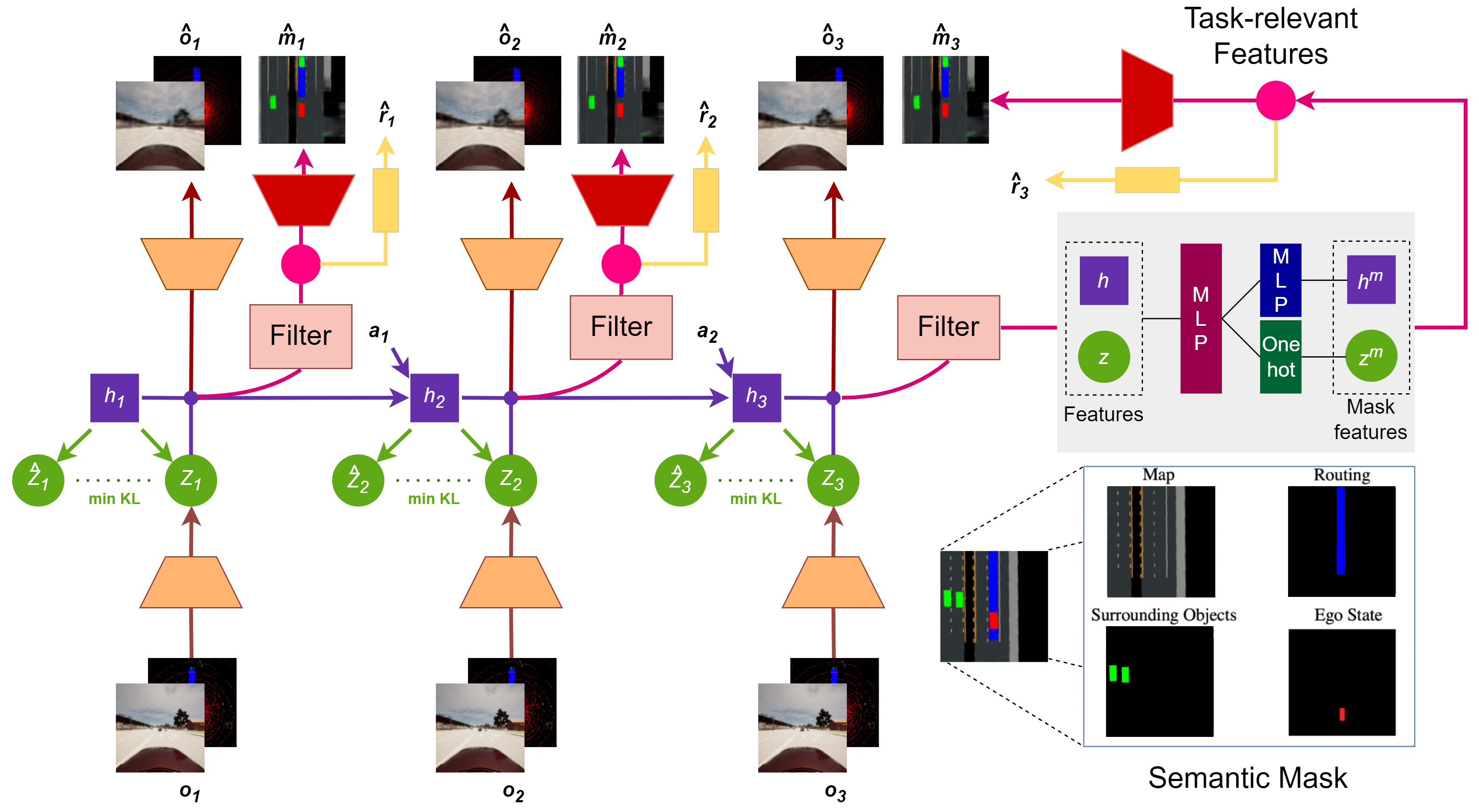
Figure 1: The overall structure of SEM2. SEM2 takes the observation $o_{t}$ from camera and lidar as input and then encodes it into latent state which contains deterministic variable $h_{t}$ and stochastic variable $z_{t}$. The original latent state is used to reconstruct the observation. The latent semantic filter extracts the driving-relevant features from latent state, and reconstructs the semantic mask $\hat{m}_{t}$ and predict the reward $\hat{r}_{t}$.

4 Semantic Masked World Model

4.1 Model Structure

As shown in Fig. 1, SEM2 consists of i) a recurrent model to extract useful information from historical information, which is implanted as a typical recurrent neural network GRUcho2014learning , ii) a representation model to encode the observation from sensor input into the latent space, iii) a transition predictor to predict the state transition, iv) a semantic filter to extract driving-relevant features, v) a mask predictor to reconstruct the semantic birdeye mask, vi) an observation predictor to reconstruct the observation and vii) a reward predictor to predict the reward given by the environment. The detailed structure of model components can be represented as:

$$\begin{array}[]{lll}\text{ Recurrent model: }&&h_{t}=f_{\phi}\left(h_{t-1},z_{t-1},a_{t-1}\right)\\ \text{ Representation model: }&&z_{t}\sim q_{\phi}\left(z_{t}\mid h_{t},o_{t}\right)\\ \text{ Transition predictor: }&&\hat{z}_{t}\sim p_{\phi}\left(\hat{z}_{t}\mid h_{t}\right)\\ \text{ Semantic filter: }&&s^{m}_{t}\sim S_{\phi}(s^{m}_{t}|h_{t},z_{t})\\ \text{ Mask predictor: }&&\hat{m_{t}}\sim p_{\phi}(\hat{m_{t}}|s^{m}_{t})\\ \text{ Observation predictor: }&&\hat{o}_{t}\sim p_{\phi}\left(\hat{o}_{t}\mid h_{t},z_{t}\right)\\ \text{ Reward predictor: }&&\hat{r}_{t}\sim p_{\phi}\left(\hat{r}_{t}\mid s^{m}_{t}\right)\\ \end{array}$$ (2)

All components are implemented as neural networks, with $\phi$ describing their combined parameter vectors. The representation model is implemented as a Convolutional Neural Network(CNNlecun1989backpropagation ) followed by a Multi-Layer Perceptron(MLP) that receives the image embedding and the deterministic recurrent state. The observation predictor is a transposed CNN, the transition and reward predictors are MLPs. The transition predictor only predicts the next latent state based on the historical information, current state and action, without using the next observation. In this way, we can predict future behavior without the need to observe or generate observations.

4.2 Semantic Filter and Mask

SEM2 takes the observations from the front camera and lidar as inputs and encodes the high-dimensional inputs into the latent space. Since the raw features encoded from the camera and lidar are susceptible to weather interference, it will reduce the robustness of the agent to weather changes. In addition, there is a large amount of driving irrelevant information in the camera images, such as the sky and tall buildings. As shown in the upper right of Fig. 1, we introduce latent semantic filter $\mathcal{S}_{\phi}(\cdot|\cdot)$ to extract the driving-relevant features. The semantic filter, which is implanted as a two-layer MLP structure, takes the latent features inferred by the recurrent neural network as input and extracts the driving-relevant features as output to reconstruct the semantic mask. The semantic mask, as shown in the lower right of Fig. 1, contains comprehensive driving-relevant information in the form of a bird-eye view that can be understood by humans, which includes the maps that represent road features, routing that represents the road a vehicle aims for, state of surrounding vehicles, and the ego state that represents the state of the ego vehicle.

4.3 Loss Function

The components of SEM2 are optimized jointly to maximize the variational lower bound proposed in hafner2020mastering , which aims to train the distributions generated by transition predictor, observation predictor, mask predictor and reward predictor to maximize the log likelihood of their corresponding targets. The mask predictor reconstructs the semantic bird-view mask via the filtered features $s^{m}_{t}$. Thus the latent filter $S$ is optimized with the part of mask log loss to minimize the error between reconstructed mask and ground truth. The loss function of the SEM2 can be derived as:

$$L(\phi){\overset{.}{=}}\underset{{q_{\phi}(s_{1:T}|a_{1:T},o_{1:T})}}{E}\left[{\sum\limits_{t=1}^{T}\underset{image~{}log~{}loss}{\underbrace{-{\ln p_{\phi}}\left(o_{t}\middle|{h_{t},z_{t}}\right)}}}\underset{mask~{}log~{}loss}{\underbrace{-{\ln p_{\phi}}\left(m_{t}\middle|{S_{\phi}(h_{t},z_{t})}\right)}}\right.$$ (3)

$$\left.\underset{reward~{}log~{}loss}{\underbrace{-{\ln p_{\phi}}\left(r_{t}\middle|{S_{\phi}(h_{t},z_{t})}\right)}}\underset{KL~{}loss}{\underbrace{+{\beta{~{}KL\left[q_{\phi}\left(z_{t}\middle|{h_{t},o_{t}}\right)\middle|\middle|p_{\phi}\left(z_{t}\middle|h_{t}\right)\right]}}}}\right]$$

The structure of SEM2 can be interpreted as a sequential VAE, where the representation model is the approximate posterior and the transition predictor is the temporal prior. The KL loss serves two purposes: it trains the prior toward the representations, and it regularizes the representations toward the prior. The driving-related feature $z_{t}^{m}$ extracted by latent semantic filters are used as the final representation, which aggregates historical information and current observations while serving as input to the policy network and value network.

4.4 Multi-source Sampler

In the process of data collection, the self-driving vehicles spend most of the time on straight roads with fewer vehicles, while the data collection on curved and crowded traffic is insufficient. This phenomenon leads to the world model unable to reconstruct the mask well, and policy learned by the world model tends to act badly under the corner case. To eliminate this gap, we proposed multi-source training method shown in Fig. 2 with a multi-source sampler.

The multi-source sampler separately collects the abnormal ending episodes in the process of interaction with the environment as the corner data set. We divide the replay buffer into three categories: common replay buffer, out-lane replay buffer and collision replay buffer. Each time the system is trained, the corner case data set is used by multi-source sampler to train the world model, so that the agent can quickly reduce the number of abnormal ending of the current scene and obtain higher returns. In the training process of SEM2, we use batches of $B=16$ sequences of fixed length $L=16$ that are sampled randomly within the stored episodes. We sample the start index of each training sequence via the multi-source sampler in both the training process and behavior learning.

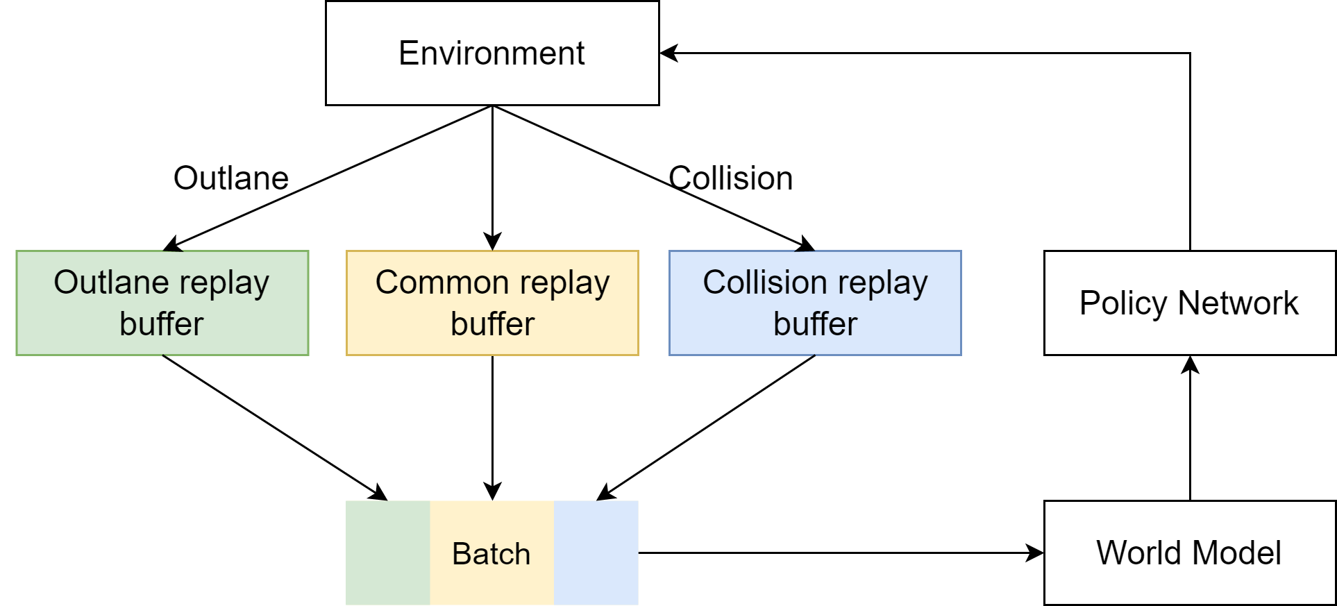
Figure 2: The structure of the multi-source sampler for the training of SEM2. In addition to the common replay buffer, there are two corner case replay buffers that save the data in out-lane cases and collision cases independently. In every iteration of the training process, we sample mini-batch from the three replay buffers in turn to contribute diverse data to support the SEM2 updating.

5 Behavior Learning

5.1 Latent imagination

We aim to learn smooth and safe driving policy through long-term imaginary trajectories unrolled by the learned world model SEM2 with high sample efficiency. For this, we propagate stochastic gradients of multi-step returns through neural network predictions of actions, states, rewards, and values using reparameterization with the help of SEM2. As shown in Fig. 3, we learn long-term behavior with SEM2 by the imaginary process, which predicts the future latent states with imagined horizon length $I$ steps from an initial state. The initial state of the process is obtained from the input images, and the subsequent hidden variables $\hat{h_{t}},\hat{z_{t}}$, actions $\hat{a}$ and rewards $\hat{r}$ are obtained from the world model predictions.

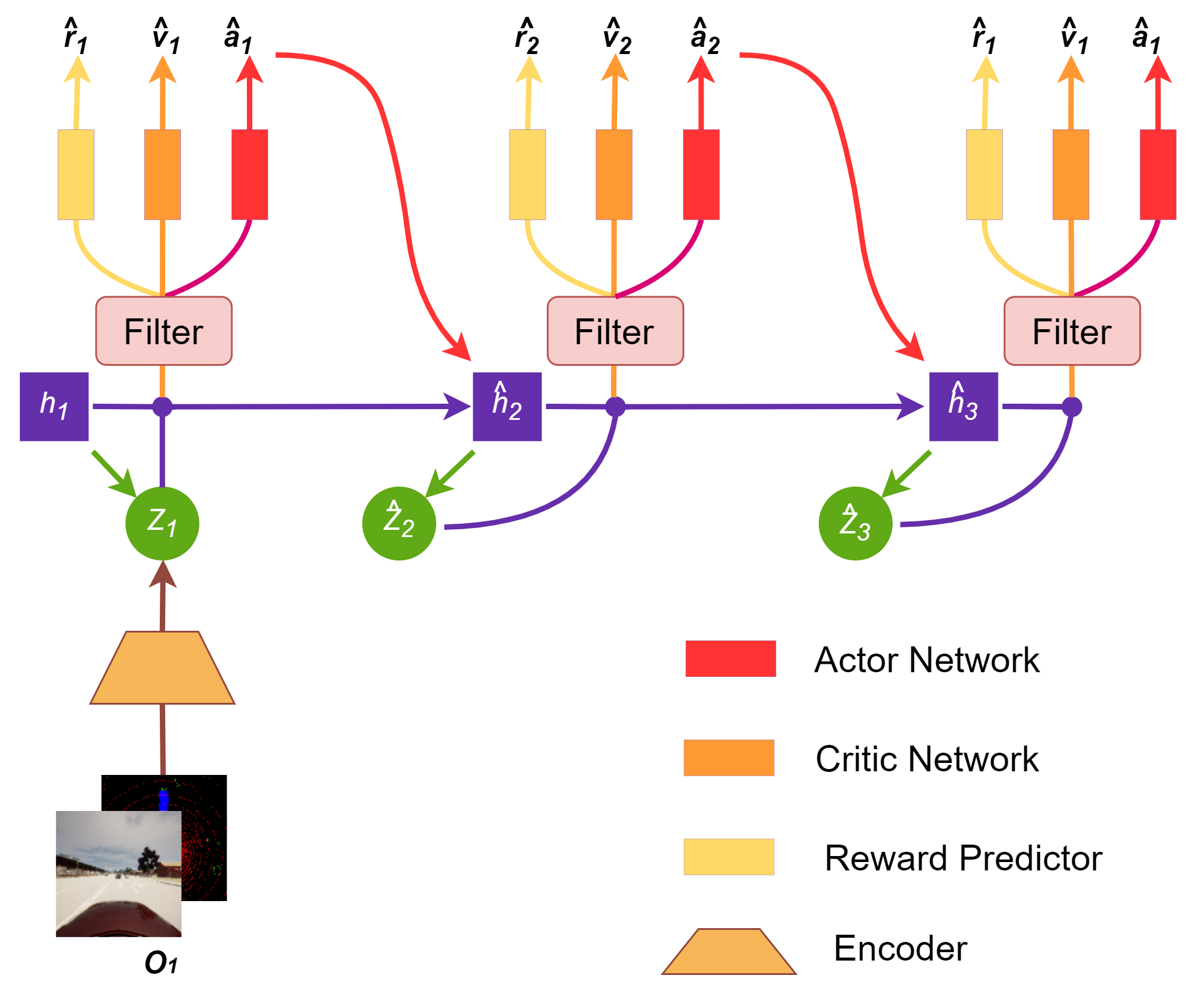
Figure 3: The semantic masked world model is used for learning a policy from trajectories imagined in the compact latent space. The trajectories start from posterior states computed during model training and predict forward by sampling actions from the actor network with the filtered driving-relevant features. The critic network learns to predict the expected rewards for each state via temporal difference learning on the imagined rewards. The actor is trained to maximize the expected rewards via the straight-through gradients of the learned world model.

5.2 Actor-Critic framework

The optimal policy is learned under an actor-critic framework with the help of the learned SEM2 model. It consists of an actor which chooses actions for maximizing the expected planning reward and a critic which predicts the future rewards. We use a stochastic actor that selects actions and a deterministic critic to learn long-horizon behaviors in the imagined MDP. The actor and critic are updated cooperatively. The actor learns to generate action according to the filtered latent state $s^{m}$ to maximize the state value predicted by the critic, which learns to estimate the actor’s cumulative rewards. The actor $\pi_{\theta}$ and critic ${v_{\varphi}}$ are represented respectively:

$$\begin{split}\text{Actor: }\quad&\hat{a_{t}}\sim\pi_{\theta}(\hat{a_{t}}|s^{m}_{t})\\ \text{Critic: }\quad&v_{\varphi}(s^{m}_{t}){\overset{.}{=}}E(\sum\limits_{k=t}^{t+I}\gamma^{k-t}r_{i})\end{split}$$ (4)

Since the features fed directly to the actor network will directly determine the quality of the generated action, in SEM2 we utilize the driving-relevant feature $s^{m}_{t}=\{h^{m}_{t},z^{m}_{t}\}$ generated by the latent semantic filter as the input of the actor network, which is highly correlated with the semantic mask and greatly reduces the interference of useless information. Through this sequential process, the agent learns to update the parameters of actor and critic networks by stochastic gradient descent method without changing the parameter of SEM2 model. As the world model is fixed during behavior learning, actor and value gradients do not affect its representations, allowing us to simulate a large number of latent trajectories efficiently on a single GPU.

The goal of the critic is to predict the state value, i.e., the discounted sum of future rewards the actor will receive. To this end, we use the TD-learning method, where the critic is trained to predict a value target, which is constructed from the intermediate rewards and the output of the critic in the later latent states. To take full advantage of the world model’s ability to make multi-step predictions and to regularize the variance of the estimates, we use the TD-$\lambda$ objective to learn the value function, which is recursively defined as follows:

$$\begin{split}&\mathcal{L_{\varphi}}\doteq\mathrm{E}_{p_{\varphi},p_{\phi}}\left[\sum_{t=1}^{I-1}\frac{1}{2}\left(v_{\varphi}\left(\hat{s}_{t}\right)-\operatorname{sg}\left(V_{t}^{\lambda}\right)\right)^{2}\right]\\ &V_{t}^{\lambda}\doteq\hat{r}_{t}+\hat{\gamma}_{t}\begin{cases}(1-\lambda)v_{\varphi}\left(\hat{s}_{t+1}\right)+\lambda V_{t+1}^{\lambda}&\text{ if }t<I\\ v_{\varphi}\left(\hat{s}_{I}\right)&\text{ if }t=I\end{cases}\end{split}$$ (5)

The TD-$\lambda$ target is a weighted average of n-step returns for different horizons. In practice, we set $\lambda=0.95$.

The actor aims to maximize the TD-$\lambda$ return predicted by the critic, while regularizing the entropy of the actor to encourage exploration. The actor and critic are both MLPs with ELU activationsclevert2015fast and are trained from the same imagined trajectories but optimize separate loss functions.

$$\mathcal{L}(\psi)\doteq\mathrm{E}_{p_{\phi},p_{\psi}}\left[\sum_{t=1}^{I-1}(\underbrace{V_{t}^{\lambda}(s^{m}_{t})}_{dynamics}\quad-\underbrace{\eta\mathrm{H}\left[a_{t}\mid\hat{s}_{t}\right]}_{\text{entropy regularizer }})\right]$$ (6)

6 Experiments

6.1 Simulation Environment Setup and Details

To further validate our method’s outperformance, we use CARLA dosovitskiy2017carla , an open-source simulator dedicated to autonomous driving research, to conduct extensive experiments. CARLA has rich weather conditions and maps that can support us testing our agents in different weather and maps to verify the environmental adaptability. All experiments were conducted on the NVIDIA RTX2080.

The map we use is $Town3$ which is a complex urban environment. The map is very close to the real city road environment, with a variety of scenarios such as tunnels, intersections, roundabouts, curves, turnaround bends, etc. The task is to drive along the complex urban environment to get rewards as high as possible in 1000 time steps without going out of bounds and colliding with 100 surroundings. The CARLA operate synchronously at 10Hz. The action composes of throttle and steer. The threshold of throttle is set to $[-3.0,3.0]$ and steer is set to $[-0.5,0.5]$.

In terms of sensors, we use a lidar and a front view camera to obtain lidar and camera image as inputs. 32-lines lidar is positioned at a height of $1.8m$. The camera has 110° FOV and is positioned at a height of $1.7m$. The size of camera, lidar and mask is set to $o_{t},m_{t}\in\left[{0,~{}255}\right]^{128\times 128\times 3}$. We train the world model with batch size $B$ 16 and batch length $L$ 16. For training the policy net, the imagined horizon $I$ is set to 4. Stochastic state $z_{t}\in R^{32\times 32}$ and deterministic state $h_{t}\in R^{2048}$. Model learning rate is $3\times 10^{-5}$ and policy learning rate is $1\times 10^{-5}$. The discount factor $\gamma$ is 0.99. SEM2 and DreamerV2 use the exact same parameters to ensure fairness.

6.2 Reward Function

Our reward function is similar to Chen et al. chen2021interpretable , which can be represented as:

$$r~{}=~{}200~{}r_{collision}+v_{lon}+10~{}r_{fast}+r_{out}-5\alpha^{2}+0.2~{}r_{lat}+0.2r_{cte}-0.1$$ (7)

The term $r_{collision}$ is set to -1 if a collision occurs. Collision, as the most avoidable condition of automatic driving, is assigned a great penalty. Ego vehicles can even take out-lane behaviors to avoid collisions when necessary. $v_{lon}$ is the longitudinal speed of the ego vehicle. The term $r_{fast}$ is set to -1 when speed of ego vehicle exceeds desired speed ($8m/s$). The term $r_{out}$ is set to -1 when cross track error (CTE) exceeds threshold ($2m$). The punishment should not be excessive, else ego vehicle tend to fall into the local optimal solution waiting for exhaustion of the episode. $\alpha$ is the steering angle of ego vehicle in rad. The term $r_{lat}$ is related to lateral acceleration computed as$-|\alpha|v_{lon}^{2}$. The term $r_{cte}$ is minus CTE to keep ego vehicle stay in the center of lane. The last constant term is added to make the ego vehicle stay in motion.

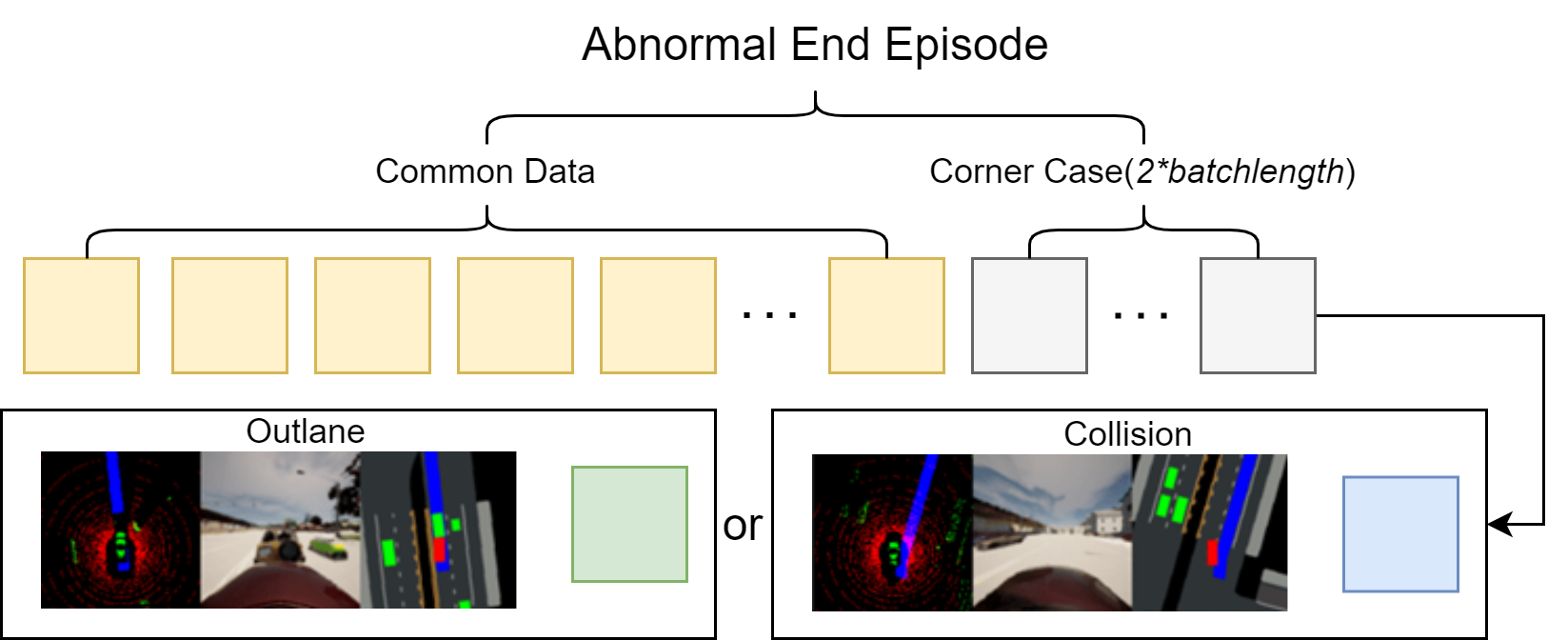
Figure 4: Multi-source data collection

6.3 Multi-source Data Collection

The corner case is defined as an abnormal end case during the data collection process. When an abnormal end occurs, the CTE of the ego vehicle is greater than $2m$ and thus out of bounds or there is a collision with a surrounding object. These two cases shown in Fig.  4 correspond to out-lane and collision. When an abnormal end occurs, the collector puts the last $2\times L$ steps of episode into the replay buffer according to the kind of end.

7 Experimental Results

The most intuitive evaluation metric for SEM2 as a reinforcement learning algorithm is average reward. We analyzed the learning curves to investigate the sample efficiency of the algorithm and the average reward under different weather to explore the adaptation of the algorithm to the environment.

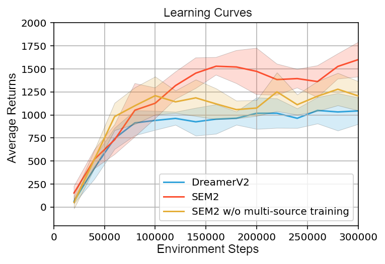
(a)

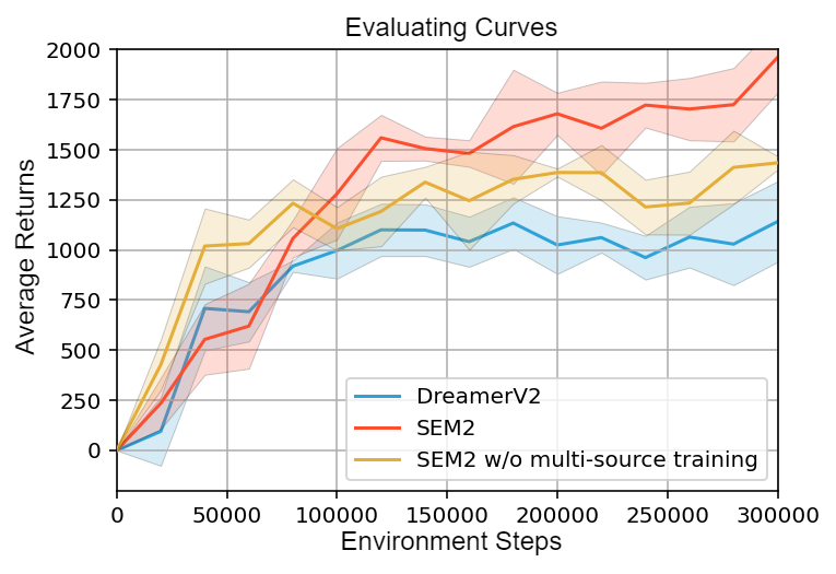
(b)

Figure 5: Learning curves and evaluating curves. The learning curves record the average return per 20,000 steps taken by the agent during training. The evaluating curves record the average return for taking 10 episodes at every 20,000 step. In the evaluation, vehicles are randomly relocated on the map for each new episode as same as in the training phase. All these average returns calculated with 5 trials. Shaded area indicates 95% confidence intervals.

7.1 Learning Curves and Evaluate Curves

All experiments are average of 5 trials and are executed for 300,000 environmental steps. Learning curves and Evaluate curves in Fig. 5 shows the performances of DreamerV2 hafner2020mastering , SEM2 without multi-source training and SEM2 with multi-source training in town3 and clear noon. We can see that our method has high sample efficiency and gets high average return. SEM2 without multi-source gets higher average return than DreamerV2 and SEM2 gets the highest average return.

7.2 Evaluate in Different Weather

Weather can have a big impact on autonomous driving, especially some bad weather. The images produced by the front view camera change with the weather, and these parts that change with the weather often contain a lot of useless features that can affect the reliability of autonomous driving. Latent filter in SEM2 extracts mask features that contains less useless information, so that SEM2 is anticipated to drive properly in different weather. In order to verify this, we evaluate our agents in five new weather conditions that agents never deal with. The five new weather conditions shown in Fig. 6 includes wet sunset, wet cloudy noon, soft rain sunset, mid rain sunset and hard rain noon. The different weathers will have huge influence on camera images. Average return calculated with 5 trials’ highest return checkpoints in five new weather is shown in Table. 1 with mean and 95% confidence intervals, SEM2 exceeds DreamerV2 in all the 5 different weathers. The comparison of SEM2 and the ablation version SEM2 without multi-source training shows that the improvement of robustness are mainly contributed by the utilizing of semantic mask while multi-source has little effect on robustness. After training, SEM2 agent is well equipped to handle many cases in complex town environments shown in Fig. 7.

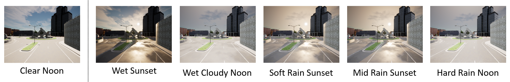
Figure 6: Screenshot of simulation under different weather

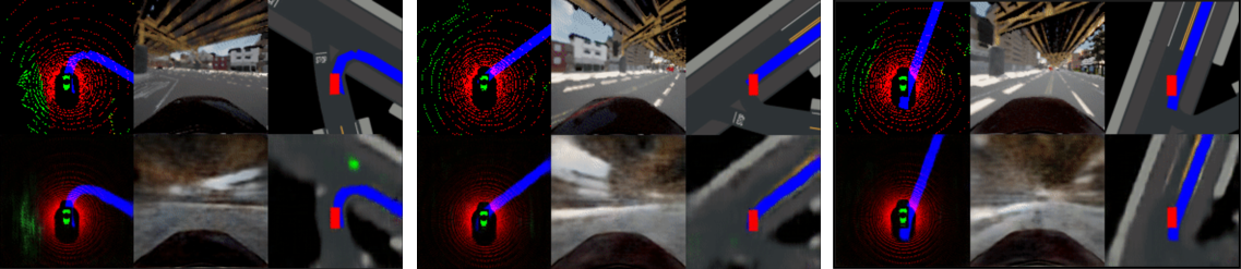
(a) Curve

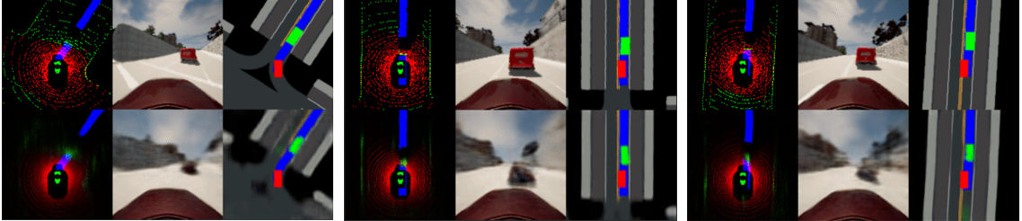
(b) Vehicle Following

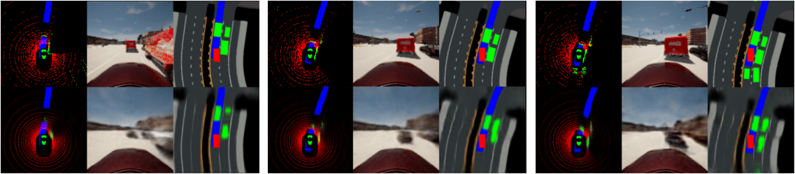
(c) Intersections

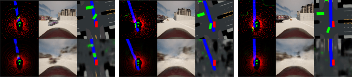
(d) Emergency

Figure 7: Cases in complex town environments

Table 1: Performance evaluation under different weather.

Weather DreamerV2 SEM2 w/o multi-source training SEM2 Wet sunset $1064.1\pm 175.5$ $1620.9\pm 148.9$ ${\bf 1692.3\pm 163.3}$ Wet cloudy noon $1078.1\pm 226.4$ ${\bf 1649.7\pm 149.3}$ $1579.3\pm 108.8$ Soft rain sunset $1313.2\pm 264.1$ $1701.1\pm 232.4$ ${\bf 1740.1\pm 207.3}$ Mid rain sunset $1181.6\pm 142.8$ $1601.5\pm 93.1$ ${\bf 1661.0\pm 124.8}$ Hard rain noon $1123.3\pm 176.4$ $1630.6\pm 121.7$ $\bf 1633.5\pm 208.7$

8 Conclusion

This paper enhances the sample efficiency and robustness of urban end-to-end autonomous driving by proposing a semantic masked recurrent world model (SEM2), which learns the transition dynamics of driving-relevant states with a latent semantic filter. The driving policy is learned by propagating analytic gradients of multi-step imagination through learned latent dynamics with SEM2 in the compact latent space. To contribute diverse scene data and prevent model collapse in corner cases, we proposed a multi-source sampler to balance the data distribution that aggregates both common driving situations and multiple corner cases in urban scenes. We trained our framework in the CARLA simulator and compared its performance with state-of-the-art comparison baselines. Experimental results demonstrate that our framework exceeds previous works in terms of sample efficiency and robustness to input permutation.

Limitation and negative societal impacts: We will validate the performance richer and more diverse scenarios in future work. We believe that our work has no negative societal impacts.

References

- (1) D. Neven, B. De Brabandere, S. Georgoulis, M. Proesmans, and L. Van Gool, “Towards end-to-end lane detection: an instance segmentation approach,” in 2018 IEEE intelligent vehicles symposium (IV). IEEE, 2018, pp. 286–291.
- (2) Y. Hou, Z. Ma, C. Liu, and C. C. Loy, “Learning lightweight lane detection cnns by self attention distillation,” in Proceedings of the IEEE/CVF international conference on computer vision, 2019, pp. 1013–1021.
- (3) K. Okamoto and P. Tsiotras, “Optimal stochastic vehicle path planning using covariance steering,” IEEE Robotics and Automation Letters, vol. 4, no. 3, pp. 2276–2281, 2019.
- (4) C. Hubmann, M. Becker, D. Althoff, D. Lenz, and C. Stiller, “Decision making for autonomous driving considering interaction and uncertain prediction of surrounding vehicles,” in 2017 IEEE Intelligent Vehicles Symposium (IV). IEEE, 2017, pp. 1671–1678.
- (5) M.-W. Park, S.-W. Lee, and W.-Y. Han, “Development of lateral control system for autonomous vehicle based on adaptive pure pursuit algorithm,” in 2014 14th International Conference on Control, Automation and Systems (ICCAS 2014). IEEE, 2014, pp. 1443–1447.
- (6) J. Chen, W. Zhan, and M. Tomizuka, “Autonomous driving motion planning with constrained iterative lqr,” IEEE Transactions on Intelligent Vehicles, vol. 4, no. 2, pp. 244–254, 2019.
- (7) M. Bojarski, D. Del Testa, D. Dworakowski, B. Firner, B. Flepp, P. Goyal, L. D. Jackel, M. Monfort, U. Muller, J. Zhang et al., “End to end learning for self-driving cars,” arXiv preprint arXiv:1604.07316, 2016.
- (8) Y. Pan, C.-A. Cheng, K. Saigol, K. Lee, X. Yan, E. Theodorou, and B. Boots, “Agile autonomous driving using end-to-end deep imitation learning,” arXiv preprint arXiv:1709.07174, 2017.
- (9) F. Codevilla, M. Müller, A. López, V. Koltun, and A. Dosovitskiy, “End-to-end driving via conditional imitation learning,” in 2018 IEEE international conference on robotics and automation (ICRA). IEEE, 2018, pp. 4693–4700.
- (10) Y. Xiao, F. Codevilla, A. Gurram, O. Urfalioglu, and A. M. López, “Multimodal end-to-end autonomous driving,” IEEE Transactions on Intelligent Transportation Systems, 2020.
- (11) S. Wang, D. Jia, and X. Weng, “Deep reinforcement learning for autonomous driving,” arXiv preprint arXiv:1811.11329, 2018.
- (12) J. Chen, B. Yuan, and M. Tomizuka, “Model-free deep reinforcement learning for urban autonomous driving,” in 2019 IEEE intelligent transportation systems conference (ITSC). IEEE, 2019, pp. 2765–2771.
- (13) J. Wu, Z. Huang, and C. Lv, “Uncertainty-aware model-based reinforcement learning with application to autonomous driving,” arXiv preprint arXiv:2106.12194, 2021.
- (14) J. Chen, S. E. Li, and M. Tomizuka, “Interpretable end-to-end urban autonomous driving with latent deep reinforcement learning,” IEEE Transactions on Intelligent Transportation Systems, 2021.
- (15) Y. Zhang, Y. Mu, Y. Yang, Y. Guan, S. E. Li, Q. Sun, and J. Chen, “Steadily learn to drive with virtual memory,” arXiv preprint arXiv:2102.08072, 2021.
- (16) D. Hafner, T. Lillicrap, J. Ba, and M. Norouzi, “Dream to control: Learning behaviors by latent imagination,” arXiv preprint arXiv:1912.01603, 2019.
- (17) D. Hafner, T. Lillicrap, M. Norouzi, and J. Ba, “Mastering atari with discrete world models,” arXiv preprint arXiv:2010.02193, 2020.
- (18) B. R. Kiran, I. Sobh, V. Talpaert, P. Mannion, A. A. Al Sallab, S. Yogamani, and P. Pérez, “Deep reinforcement learning for autonomous driving: A survey,” IEEE Transactions on Intelligent Transportation Systems, 2021.
- (19) V. Mnih, K. Kavukcuoglu, D. Silver, A. A. Rusu, J. Veness, M. G. Bellemare, A. Graves, M. Riedmiller, A. K. Fidjeland, G. Ostrovski et al., “Human-level control through deep reinforcement learning,” nature, vol. 518, no. 7540, pp. 529–533, 2015.
- (20) S. Levine, C. Finn, T. Darrell, and P. Abbeel, “End-to-end training of deep visuomotor policies,” The Journal of Machine Learning Research, vol. 17, no. 1, pp. 1334–1373, 2016.
- (21) D. Silver, A. Huang, C. J. Maddison, A. Guez, L. Sifre, G. Van Den Driessche, J. Schrittwieser, I. Antonoglou, V. Panneershelvam, M. Lanctot et al., “Mastering the game of go with deep neural networks and tree search,” nature, vol. 529, no. 7587, pp. 484–489, 2016.
- (22) D. Silver, J. Schrittwieser, K. Simonyan, I. Antonoglou, A. Huang, A. Guez, T. Hubert, L. Baker, M. Lai, A. Bolton et al., “Mastering the game of go without human knowledge,” nature, vol. 550, no. 7676, pp. 354–359, 2017.
- (23) P. Wolf, C. Hubschneider, M. Weber, A. Bauer, J. Härtl, F. Dürr, and J. M. Zöllner, “Learning how to drive in a real world simulation with deep q-networks,” in 2017 IEEE Intelligent Vehicles Symposium (IV). IEEE, 2017, pp. 244–250.
- (24) H. Ma, J. Chen, S. Eben, Z. Lin, Y. Guan, Y. Ren, and S. Zheng, “Model-based constrained reinforcement learning using generalized control barrier function,” in 2021 IEEE/RSJ International Conference on Intelligent Robots and Systems (IROS). IEEE, 2021, pp. 4552–4559.
- (25) J. Kim and J. Canny, “Interpretable learning for self-driving cars by visualizing causal attention,” in Proceedings of the IEEE international conference on computer vision, 2017, pp. 2942–2950.
- (26) Y. Guan, Y. Ren, S. E. Li, H. Ma, J. Duan, and B. Cheng, “Integrated decision and control: Towards interpretable and efficient driving intelligence,” arXiv preprint arXiv:2103.10290, 2021.
- (27) D. Ha and J. Schmidhuber, “Recurrent world models facilitate policy evolution,” Advances in neural information processing systems, vol. 31, 2018.
- (28) D. Hafner, T. Lillicrap, I. Fischer, R. Villegas, D. Ha, H. Lee, and J. Davidson, “Learning latent dynamics for planning from pixels,” in International conference on machine learning. PMLR, 2019, pp. 2555–2565.
- (29) A. X. Lee, A. Nagabandi, P. Abbeel, and S. Levine, “Stochastic latent actor-critic: Deep reinforcement learning with a latent variable model,” Advances in Neural Information Processing Systems, vol. 33, pp. 741–752, 2020.
- (30) G. Zhu, M. Zhang, H. Lee, and C. Zhang, “Bridging imagination and reality for model-based deep reinforcement learning,” Advances in Neural Information Processing Systems, vol. 33, pp. 8993–9006, 2020.
- (31) K. Cho, B. Van Merriënboer, C. Gulcehre, D. Bahdanau, F. Bougares, H. Schwenk, and Y. Bengio, “Learning phrase representations using rnn encoder-decoder for statistical machine translation,” arXiv preprint arXiv:1406.1078, 2014.
- (32) Y. LeCun, B. Boser, J. S. Denker, D. Henderson, R. E. Howard, W. Hubbard, and L. D. Jackel, “Backpropagation applied to handwritten zip code recognition,” Neural computation, vol. 1, no. 4, pp. 541–551, 1989.
- (33) D.-A. Clevert, T. Unterthiner, and S. Hochreiter, “Fast and accurate deep network learning by exponential linear units (elus),” arXiv preprint arXiv:1511.07289, 2015.
- (34) A. Dosovitskiy, G. Ros, F. Codevilla, A. Lopez, and V. Koltun, “Carla: An open urban driving simulator,” in Conference on robot learning. PMLR, 2017, pp. 1–16.