Spectrally-Corrected and Regularized LDA for Spiked Model

Abstract

This paper proposes an improved linear discriminant analysis called spectrally-corrected and regularized LDA (SRLDA). This method integrates the design ideas of the sample spectrally-corrected covariance matrix and the regularized discriminant analysis. The SRLDA method specially designed for classification problems is under the assumption that the covariance matrix follows a spiked model. Through the real and simulated data analysis, our proposed classifier outperforms the classical R-LDA and can be as competitive as the KNN and SVM classifiers while requiring lower computational complexity. Furthermore, this paper generalizes the limiting result of the angle between true and estimated eigenvectors given in Paul 2007 to small spiked eigenvalues and weakens the multivariate normal distribution assumption to the limited $4$-th moment ones.

1 Introduction

The statistics problem treated here is assigning a $p$-dimensional observation ${\mathbf{x}}=\left(x_{1},x_{2},\dots,x_{p}\right)^{\prime}$ into one of two classes or groups $\Pi_{i}$ $(i=0,1)$. The classes are assumed to have Gaussian distributions with the same covariance matrix. Since R.A. Fisher [16] originally proposed Linear Discriminant Analysis (LDA) based classifiers in 1936, Fisher’s LDA has been one of the most classical techniques for classification tasks and is still used routinely in applications. Under the support of the labeled sample sets, Fisher’s discriminant rule directs us to allocate ${\mathbf{x}}$ into $\Pi_{0}$ if

$$W^{LDA}(\overline{{\mathbf{x}}}_{0},\overline{{\mathbf{x}}}_{1},{\mathbf{S}},{\mathbf{x}})=\left({\mathbf{x}}-\frac{\overline{{\mathbf{x}}}_{0}+\overline{{\mathbf{x}}}_{1}}{2}\right)^{T}{\mathbf{S}}^{-1}\left(\overline{{\mathbf{x}}}_{0}-\overline{{\mathbf{x}}}_{1}\right)-\log\frac{\pi_{1}}{\pi_{0}}>0,$$ (1.1)

and into $\Pi_{1}$ otherwise, where $\pi_{i}$ is the prior probability corresponding to $\Pi_{i}$ ($i=0,1$). Here $\overline{{\mathbf{x}}}_{1}$ and $\overline{{\mathbf{x}}}_{2}$ are the sample mean vectors of two classes, and ${\mathbf{S}}$ is the pooled sample covariance matrix. LDA has a long and successful history. From the first use of taxonomic classification by [16], LDA-Fisher-based classification and recognition systems have been used in many applications, including detection [50], speech recognition [49], cancer genomics [28], and face recognition [46].

In the classic asymptotic approach, $W^{LDA}(\overline{{\mathbf{x}}}_{0},\overline{{\mathbf{x}}}_{1},{\mathbf{S}},{\mathbf{x}})$ is the consistent estimation of Fisher’s LDA function. However, it is not generally helpful in situations where the dimensionality of the observations is of the same order of magnitude as the sample size $(n\rightarrow\infty,p\rightarrow\infty,$ and $p/n\rightarrow J>0)$. In this asymptotic scenario, the Fisher discriminant rule performs poorly due to the sample covariance matrix diverging from the population’s one severely. There are several papers developing different approaches to handling the high-dimensionality issue in the estimation of the covariance matrix, which can be divided into two schools. The first suggests building on the additional knowledge in the estimation process, such as sparseness, graph model, or factor model [6, 7, 13, 27, 40, 42, 43]. The second recommends correcting the spectrum of the sample covariance [33], such as the shrinkage estimator in [11, 31, 32], and regularized technologic in [4, 12, 45, 53]. The Spectrally-Corrected and Regularized LDA (SRLDA) given in this paper belong to the second school, which integrates the design ideas of the sample spectrally-corrected covariance matrix [33] and the regularized discriminant analysis [19] to improve the LDA estimation in high-dimensional settings.

In this paper, a novel approach is proposed under the assumption that all but a finite number of eigenvalues of the population covariance matrix are the same, which is known as the spiked covariance model in [24]. This model could be and has been used in many real applications, such as detection speech recognition [20, 24], mathematical financial [29, 30, 34, 36, 39], wireless communication [47], physics of mixture [44], EEG signals [10, 15] and data analysis and statistical learning [21]. Based on some theoretical and applied results of the spiked covariance model([2, 3, 5, 26, 38]), we suppose the population eigenvalues can be estimated reasonably. Then consider a class of covariance matrix estimators that follow the same spiked structure, that is written as a finite rank perturbation of a scaled identity matrix. The sample eigenvectors of the extreme sample eigenvalues provide the directions of the low-rank perturbation and the corresponding eigenvalues are corrected to population one and regularized by the common parameter. In this way, we not only preserve the spiked structure as much as possible but also reduce the number of undetermined parameters compared with that in [45].

In this paper, the design parameters are chosen so that an approximation of the misclassification rate is minimized and can be obtained in the corresponding closed form without using the standard cross-validation approach, by which a lower complexity and a higher classification performance are presented and the computational cost is also reduced compared to the classical R-LDA in [12]. By the real data analysis, it is shown that the proposed classifier outperforms other popular classification techniques such as improved LDA (I-LDA) in [45], support vector machine (SVM), and $k$-nearest neighbors (KNN).

The remaining of this paper is organized as follows: In Section 2, we describe binary classification and SRLDA classifier. In Section 3, the consistent estimator of the true error is provided. We improve the SRLDA classifier with optimal intercept in Section 4. In Section 5, we study the performance of the SRLDA by numerical simulations and provide some conclusions in Section 6.

2 Binary Classification and SRLDA Classifier

On the basis of the analysis framework in [53], some modeling assumptions are restated and made throughout the paper. First, we employ separate (stratified) sampling: $n=n_{0}+n_{1}$ sample points are collected to constitute the sample ${\mathbf{C}}$ in $R^{p}$, where, given $n$, $n_{0}$ and $n_{1}$ are determined (not random) and where ${\mathbf{C}}_{0}=\{{\bf x}_{1},{\bf x}_{2},...,{\bf x}_{n_{0}}\}$ and ${\mathbf{C}}_{1}=\{{\bf x}_{n_{0}+1},{\bf x}_{n_{0}+2},...,{\bf x}_{n}\}$ are randomly selected from populations $\Pi_{0}$ and $\Pi_{1}$, respectively. Separate sampling is very common in biomedical applications, where data from two classes are collected without reference to the other, for instance, to discriminate two types of tumors or to distinguish a normal from a pathological phenotype.

A second assumption is that the classes possess a common covariance matrix. $\Pi_{i}$ follows a multivariate Gaussian distribution $N({{\bm{\mu}}}_{i},{{\bm{\Sigma}}})$, for $i=0,1$, where ${{\bm{\Sigma}}}$ is nonsingular. Although it does not fully correspond to reality, the LDA still often performs better than quadratic discriminant analysis (QDA) in most cases, even with different covariances, because of the advantage of its estimation method [41].

In this paper, we improve the LDA classifier in the particular scenarios, as the third assumption, wherein ${\bm{\Sigma}}$ takes the following particular form [2]:

$${\bm{\Sigma}} = \sigma^{2}\left({\mathbf{I}}_{p}+\sum_{j\in\mathbb{I}}\lambda_{j}{\mathbf{v}}_{j}{\mathbf{v}}_{j}^{T}\right),$$ (2.1)

where $\mathbb{I}=:\mathbb{I}_{1}\cup\mathbb{I}_{2}$, $\mathbb{I}_{1}:=\{1,\dots,r_{1}\}$, $\mathbb{I}_{2}:=\{-r_{2},\dots,-1\}$, $\sigma^{2}>0$, $r=r_{1}+r_{2}$, $\lambda_{1}\geq\cdots\geq\lambda_{r_{1}}>0>\lambda_{-r_{2}}\geq\cdots\geq\lambda_{-1}>-1$ and ${\mathbf{v}}_{i}$ ($i\in\mathbb{I}$) are orthogonal. The above model is the so-called spiked model and is encountered in many real applications, among which detection [52], EEG signals [10, 15], and financial econometrics [29, 37] are the best representatives. For the sake of simplicity, we assume that $\sigma^{2}$, $r_{1}$, $r_{2}$, and $\lambda_{i}$ ($i\in I$) are perfectly known. In practice, one can resort to the existing efficient algorithms available in the literature [2, 14, 17, 23, 25, 26, 29, 36, 48] for the estimation of these parameters. In our numerical simulations, we have used the method of [2, 23, 26].

In this paper, the spectrally-corrected method is to correct the spectral elements of the sample covariance matrix to those of $\Sigma$. Start the eigen decomposition of the pooled covariance matrix as

$${\mathbf{S}}=\sum_{j=1}^{p}l_{j}{\mathbf{u}}_{j}{\mathbf{u}}_{j}^{T},$$ (2.2)

with $l_{j}$ being the $j$-th largest eigenvalue and ${\mathbf{u}}_{j}$ its corresponding eigenvector. Then correct $l_{j}$ to the corresponding one of $\Sigma$ as following:

$${\widetilde{\mathbf{S}}} = \sigma^{2}\left({\mathbf{I}}_{p}+\sum_{j\in{\mathbb{I}}}\lambda_{j}{\mathbf{u}}_{j}{\mathbf{u}}_{j}^{T}\right),$$ (2.3)

where ${\mathbf{u}}_{j}\triangleq{\mathbf{u}}_{p+1+j}$ for $j\in\mathbb{I}_{2}$. In (2.3), ${\widetilde{\mathbf{S}}}$ is totaly same as (2.1) except the spiked eigen vectors. In this way, the original structure of $\Sigma$ is preserved as much as possible, but the disadvantage is that $\widetilde{{\mathbf{S}}}$ is a biased estimator of $\Sigma$ because of the bias of sample spiked eigenvectors from that of the population. How do deal with the bias? R-LDA [18, 53] method inspires us to introduce regularization parameters for the sample spiked matrix for LDA. Then we have the spectrally-corrected and regularized discriminant analysis (SRLDA) function, that is

$$W^{SRLDA}\left(\overline{{\mathbf{x}}}_{0},\overline{{\mathbf{x}}}_{1},{\widetilde{\mathbf{H}}},{\mathbf{x}}\right)=\sigma^{-2}\left({\mathbf{x}}-\frac{\overline{{\mathbf{x}}}_{0}+\overline{{\mathbf{x}}}_{1}}{2}\right)^{T}{\widetilde{\mathbf{H}}}\left(\overline{{\mathbf{x}}}_{0}-\overline{{\mathbf{x}}}_{1}\right),$$ (2.4)

where

$${\widetilde{\mathbf{H}}} = \left({\mathbf{I}}_{p}+\gamma_{1}\sum_{j\in{\mathbb{I}}_{1}}\lambda_{j}{\mathbf{u}}_{j}{\mathbf{u}}_{j}^{T}+\gamma_{2}\sum_{j\in{\mathbb{I}}_{2}}\lambda_{j}{\mathbf{u}}_{j}{\mathbf{u}}_{j}^{T}\right)^{-1}.$$ (2.5)

Here $\gamma_{1}$ and $\gamma_{2}$ are designed parameters to be optimal. We assume that

$$\left(\gamma_{1},\gamma_{2}\right)\in\mathbb{A}=\left\{\gamma_{1},\gamma_{2}:0<\gamma_{1},\gamma_{2}<M,\gamma_{2}\notin\cup_{j\in{\mathbb{I}}_{2}}U\left(|\lambda_{j}|^{-1},\delta\right)\right\}$$ (2.6)

for some $M,\delta>0$, where $U\left(|\lambda_{j}|^{-1},\delta\right)=\left\{x:\left|x-|\lambda_{j}|^{-1}\right|<\delta\right\}$. From a practical point of view, we only need to assume that $\gamma_{2}\notin\cup_{j\in{\mathbb{I}}_{2}}U\left(|\lambda_{j}|^{-1},\delta\right)$ to ensure that the spectral norm of ${\widetilde{\mathbf{H}}}$ is bounded. However, the restriction to range $\mathbb{A}$ is needed later for the proof of the uniform convergence results. The designed SRLDA classifier is then given by

$$\psi_{n}^{SRLDA}=\left\{\begin{array}[]{ll}1,&\hbox{if $W^{SRLDA}\left(\overline{{\mathbf{x}}}_{0},\overline{{\mathbf{x}}}_{1},{\widetilde{\mathbf{H}}},{\mathbf{x}}\right)\leq c$;}\\ 0,&\hbox{if $W^{SRLDA}\left(\overline{{\mathbf{x}}}_{0},\overline{{\mathbf{x}}}_{1},{\widetilde{\mathbf{H}}},{\mathbf{x}}\right)>c$,}\end{array}\right.$$ (2.9)

where $c=\log(\pi_{1}/\pi_{0})$. Given $\overline{{\mathbf{x}}}_{0},\overline{{\mathbf{x}}}_{1},{\widetilde{\mathbf{S}}}$, the error contributed by class $i$ ($=0$ or $1$), is defined by the probability of misclassification,

$$\varepsilon_{i}^{SRLDA} = P\left((-1)^{i}W^{SRLDA}\left(\overline{{\mathbf{x}}}_{0},\overline{{\mathbf{x}}}_{1},{\widetilde{\mathbf{H}}},{\mathbf{x}}\right)\leq(-1)^{i}c\left|{\mathbf{x}}\in\Pi_{i},\overline{{\mathbf{x}}}_{0},\overline{{\mathbf{x}}}_{1},{\widetilde{\mathbf{H}}}\right.\right)$$ (2.10)

$$= \Phi\left(\frac{(-1)^{i+1}G\left({\bm{\mu}}_{i},\overline{{\mathbf{x}}}_{0},\overline{{\mathbf{x}}}_{1},{\widetilde{\mathbf{H}}}\right)+(-1)^{i}\sigma^{2}c}{\sqrt{D\left(\overline{{\mathbf{x}}}_{0},\overline{{\mathbf{x}}}_{1},{\widetilde{\mathbf{H}}},{\bm{\Sigma}}\right)}}\right),$$

where $\Phi(\cdot)$ denotes the cumulative distribution function of a standard normal random variable and

$$G\left({\bm{\mu}}_{i},\overline{{\mathbf{x}}}_{0},\overline{{\mathbf{x}}}_{1},{\widetilde{\mathbf{H}}}\right) = \left({\bm{\mu}}_{i}-\frac{\overline{{\mathbf{x}}}_{0}+\overline{{\mathbf{x}}}_{1}}{2}\right)^{T}{\widetilde{\mathbf{H}}}\left(\overline{{\mathbf{x}}}_{0}-\overline{{\mathbf{x}}}_{1}\right),$$ (2.11)

$$D\left(\overline{{\mathbf{x}}}_{0},\overline{{\mathbf{x}}}_{1},{\widetilde{\mathbf{H}}},{\bm{\Sigma}}\right) = \left(\overline{{\mathbf{x}}}_{0}-\overline{{\mathbf{x}}}_{1}\right)^{T}{\widetilde{\mathbf{H}}}{\bm{\Sigma}}{\widetilde{\mathbf{H}}}\left(\overline{{\mathbf{x}}}_{0}-\overline{{\mathbf{x}}}_{1}\right).$$ (2.12)

The true error of $\psi_{n}^{SRLDA}$ is expressed as:

$$\varepsilon^{SRLDA}=\pi_{0}\varepsilon_{0}^{SRLDA}+\pi_{1}\varepsilon_{1}^{SRLDA}.$$ (2.13)

3 Consistent Estimate of the True Error and Parameter Optimization

In this section, we derive a consistent estimator of the true error of SRLDA based on random matrix theory, which is used to obtain optimal parameters. The theoretical optimal $\gamma_{1},\gamma_{2}$ is chosen to minimize the total misclassification rate:

$$\gamma_{1}^{*},\gamma_{2}^{*}=\mathop{\arg\min}\limits_{\left(\gamma_{1},\gamma_{2}\right)\in\mathbb{A}}\varepsilon^{SRLDA}(\gamma_{1},\gamma_{2}),$$ (3.1)

and its consistent estimate is responsible for the acquisition of optimal empirical parameters. Under the asymptotic growth regime, the following assumptions will help us to build a consistent estimate.

Assumption 3.1.

$p,n_{0},n_{1}\rightarrow\infty$, and the following limits exist: $\frac{p}{n_{0}}\rightarrow J_{0}>0$, $\frac{p}{n_{1}}\rightarrow J_{1}>0$ and $\frac{p}{n}\rightarrow J<1$ where $n=n_{0}+n_{1}$.

Assumption 3.1 is a norm assumption in the framework of the high dimensional random matrix theory, where an estimator is constructed such that it converges to the actual parameter.

Assumption 3.2.

$r_{1}$ and $r_{2}$ are fixed and $\lambda_{1}>\cdots>\lambda_{r_{1}}>\sqrt{J}>0>-\sqrt{J}>\lambda_{-r_{2}}>\cdots>\lambda_{-1}>-1$, independently of $p$ and $n$.

Assumption 3.2 is fundamental in our analysis since it guarantees, as standard results from random matrix theory, the one-to-one mapping between the sample eigen-values and the unknown population one. In fact, when $\lambda_{j}>\sqrt{J}$ (or $-1<\lambda_{j}<-\sqrt{J}$), $\lambda_{j}$ can be consistently estimated for $j\in\mathbb{I}$.

Assumption 3.3.

$\|{\bm{\mu}}_{i}\|$ has a bounded Euclidean norm, that is $\|{\bm{\mu}}_{i}\|=O(1)$, $i=0,1$.

Assumption 3.4.

The spectral norm of $\Sigma$ is bounded, that is $\|{\bm{\Sigma}}\|=O(1)$.

Theorem 1.

Under Assumptions 3.1 to 3.4, for any $\left(\gamma_{1},\gamma_{2}\right)\in{\mathbb{A}}$ and $k=0$ (or $1$), we have

$$\left|G\left({\bm{\mu}}_{k},\overline{{\mathbf{x}}}_{0},\overline{{\mathbf{x}}}_{1},{\widetilde{\mathbf{H}}}\right)-\frac{(-1)^{k}}{2}\|{\bm{\mu}}\|^{2}\overline{G}(\gamma_{1},\gamma_{2})+\frac{\sigma^{2}}{2}\left(\frac{p}{n_{0}}-\frac{p}{n_{1}}\right)\right|\xrightarrow{a.s.}0,$$ (3.2)

$$\left|D\left(\overline{{\mathbf{x}}}_{0},\overline{{\mathbf{x}}}_{1},{\widetilde{\mathbf{H}}},{\bm{\Sigma}}\right)-\sigma^{2}\|{\bm{\mu}}\|^{2}\overline{D}(\gamma_{1},\gamma_{2})-\sigma^{4}\left(\frac{p}{n_{0}}+\frac{p}{n_{1}}\right)\right|\xrightarrow{a.s.}0,$$ (3.3)

uniformly, where

$$\overline{G}\left(\gamma_{1},\gamma_{2}\right) = 1-\sum_{i=1,2}\sum_{j\in{\mathbb{I}}}a_{j}b_{j}\gamma_{i,j}\delta_{i,j},$$ (3.4)

$$\overline{D}(\gamma_{1},\gamma_{2}) = 1+\sum_{j\in{\mathbb{I}}}\lambda_{j}b_{j}-2\sum_{i=1,2}\sum_{j\in{\mathbb{I}}}\left(\lambda_{j}+1\right)a_{j}b_{j}\gamma_{i,j}\delta_{i,j}$$ (3.5)

$$+\sum_{i=1,2}\sum_{j\in{\mathbb{I}}}a_{j}b_{j}\left(\lambda_{j}a_{j}+1\right)\gamma_{i,j}^{2}\delta_{i,j}.$$

Here

$${\bm{\mu}}={\bm{\mu}}_{0}-{\bm{\mu}}_{1},\;\;\gamma_{i,j}=\frac{\gamma_{i}\lambda_{j}}{1+\gamma_{i}\lambda_{j}},\;\;a_{j}=\frac{\lambda_{j}^{2}-c}{\lambda_{j}(\lambda_{j}+c)},\;\mbox{and }\;b_{j}=\frac{\left({\bm{\mu}}^{T}{\mathbf{v}}_{j}\right)^{2}}{\|{\bm{\mu}}\|^{2}},$$

for $i=1,2$, $j\in{\mathbb{I}}$ and

$$\delta_{i,j}=\left\{\begin{array}[]{ll}1,&\hbox{$i=1,j>0$ or $i=2,j<0$;}\\ 0,&\hbox{otherwise.}\end{array}\right.$$

Proof.

See Appendix A.

According to Theorem 1, a deterministic equivalent of the global misclassification rate can be obtained as:

$$\varepsilon^{SRLDA}(\gamma_{1},\gamma_{2})-\overline{\varepsilon}^{SRLDA}(\gamma_{1},\gamma_{2})\xrightarrow{a.s.}0,$$

where

$$\overline{\varepsilon}^{SRLDA}(\gamma_{1},\gamma_{2})=\pi_{0}\Phi\left(-\frac{\overline{G}(\gamma_{1},\gamma_{2})-\eta}{2\sqrt{\alpha}\sqrt{\overline{D}(\gamma_{1},\gamma_{2})+\zeta}}\right)+\pi_{1}\Phi\left(-\frac{\overline{G}(\gamma_{1},\gamma_{2})+\eta}{2\sqrt{\alpha}\sqrt{\overline{D}(\gamma_{1},\gamma_{2})+\zeta}}\right).$$ (3.7)

Here $\alpha=\frac{\sigma^{2}}{\|{\bm{\mu}}\|^{2}}$, $\eta=\alpha\left(\frac{p}{n_{0}}-\frac{p}{n_{1}}+2c\right)$ and $\zeta=\alpha\left(\frac{p}{n_{0}}+\frac{p}{n_{1}}\right)$. (3.7) is similar to (17) given in [45], but here are only two regularized parameters that are optimized on a more specific bounded set in Theorem 3, compared with that of [45].

Theorem 2.

Under the setting of Assumptions 3.1 to 3.4, we have

$${\varepsilon}^{SRLDA}(\gamma_{1},\gamma_{2})-\overline{\varepsilon}^{SRLDA}(\gamma_{1},\gamma_{2})\xrightarrow{a.s.}0,\;\;\;\forall\left(\gamma_{1},\gamma_{2}\right)\in\mathbb{A},$$ (3.8)

uniformly, where $\overline{\varepsilon}^{SRLDA}$ and $\mathbb{A}$ are given in (3.7) and (2.6) respectively.

Proof.

According Theorem 1, (6.10) and the continuity of $\Phi$, (3.8) holds naturally.

Theorem 3.

Under the setting of Assumptions 3.1 to 3.4, the optimal parameters ${\gamma_{1}^{*},\gamma_{2}^{*}}$ that minimize $\overline{\varepsilon}^{SRLDA}(\gamma_{1},\gamma_{2})$ are given by:

$$\gamma_{1}^{*}=\frac{\omega_{1}^{*}}{(1-\omega_{1}^{*})\lambda_{1}}\;\;\mbox{and}\;\;\gamma_{2}^{*}=\frac{-\omega_{2}^{*}}{(1-\omega_{2}^{*})\lambda_{-1}},$$

where $(\omega_{1}^{*},\omega_{2}^{*})$ is the minimizer of the function $f(\omega_{1},\omega_{2})$, $\left(\omega_{1},\omega_{2}\right)\in{{\mathbb{B}}}$, given by

$$\pi_{0}\Phi\left(-\frac{1}{2\sqrt{\alpha}}\frac{\widetilde{G}(\omega_{1},\omega_{2})-\eta}{\sqrt{\widetilde{D}(\omega_{1},\omega_{2})+\zeta}}\right)+\pi_{1}\Phi\left(-\frac{1}{2\sqrt{\alpha}}\frac{\widetilde{G}(\omega_{1},\omega_{2})+\eta}{\sqrt{\widetilde{D}(\omega_{1},\omega_{2})+\zeta}}\right).$$

Here ${\mathbb{B}}=\left\{(\omega_{1},\omega_{2}):0<\omega_{1},\omega_{2}<1,\omega_{2}\neq\left(1+\lambda_{j}/\lambda_{-1}\right)^{-1},j\in{\mathbb{I}}_{2}\right\}$,

$$\widetilde{G}\left(\omega_{1},\omega_{2}\right) = 1-\sum_{i=1,2}\sum_{j\in{\mathbb{I}}}a_{j}b_{j}\gamma_{i,j}\delta_{i,j},$$

$$\widetilde{D}(\omega_{1},\omega_{2}) = 1+\sum_{j\in{\mathbb{I}}}\lambda_{j}b_{j}-2\sum_{i=1,2}\sum_{j\in{\mathbb{I}}}\left(\lambda_{j}+1\right)a_{j}b_{j}\gamma_{i,j}\delta_{i,j}$$

$$+\sum_{i=1,2}\sum_{j\in\mathbb{I}}a_{j}b_{j}\left(\lambda_{j}a_{j}+1\right)\gamma_{i,j}^{2}\delta_{i,j},$$

$$\gamma_{1,j} = \frac{\omega_{1}\lambda_{j}}{(1-\omega_{1})\lambda_{1}+\omega_{1}\lambda_{j}},\;\;\;j\in{\mathbb{I}}_{1},$$

$$\gamma_{2,j} = \frac{-\omega_{2}\lambda_{j}}{(1-\omega_{2})\lambda_{-1}-\omega_{2}\lambda_{j}},\;\;\;j\in{\mathbb{I}}_{2}.$$

And $\eta$ and $\zeta$ are defined in Theorem 1.

Proof.

See Appendix B.

Theorem 4.

Under Assumptions 3.1 to 3.4, for any deterministic unit vector ${\mathbf{w}}\in S_{\mathbb{R}}^{p-1}$, we have

$$\left\langle{\mathbf{w}},{\mathbf{u}}_{j}{\mathbf{u}}_{j}^{T}{\mathbf{w}}\right\rangle\xrightarrow{a.s.}\dfrac{\lambda_{j}^{2}-J}{\lambda_{j}(\lambda_{j}+J)}\left\langle{\mathbf{w}},{\mathbf{v}}_{j}{\mathbf{v}}_{j}^{T}{\mathbf{w}}\right\rangle,$$ (3.9)

for $j\in{\mathbb{I}}$.

Theorem 4 generalizes the limiting result of the angle between true and estimated eigenvectors given in [38] to small spiked eigenvalues and weaken the multivariate normal distribution assumption to the limited $4$-th moment ones. That is following:

Assumption 3.5.

Let ${\mathbf{Z}}_{n}=\left[{\mathbf{z}}_{1},{\mathbf{z}}_{2},...,{\mathbf{z}}_{n}\right]=(z_{ij})$ denotes a $p\times(n_{0}+n_{1})$ random matrix such that the entries $z_{ij}$s are independent and identically distributed (i.i.d) real random variables satisfying $\mathbb{E}z_{ij}=0$, $\mathbb{E}z_{ij}^{2}=1$, and $\mathbb{E}|z_{ij}|^{4}<\infty$. Assume ${\mathbf{X}}_{n}$ is a $p\times(n_{0}+n_{1})$ matrix obtained by

$${\mathbf{X}}_{n}=\left[{\bm{\mu}}_{0}{\mathbf{1}}_{n_{0}}^{T},{\bm{\mu}}_{1}{\mathbf{1}}_{n_{1}}^{T}\right]+{\bm{\Sigma}}^{1/2}{\mathbf{Z}}_{n}.$$

The proof of Theorem 4 holds under Assumption 3.5 instead of the multivariate normal distribution assumption.

4 Improved SRLDA with optimal intercept

The intercept part of (1.1) is another important parameter that affects the misclassification rate. Since the empirical estimation of the intercept part always causes severe bias in unbalanced classes and high-dimensional settings, it is necessary to consider bias correction, which is now a general procedure to minimize the misclassification rate such as [8, 22, 51]. In this section, we apply the bias correction procedure to the improved LDA classifier and name the classifier ”OI-SRLDA” to refer to the optimal-intercept-SRLDA classifier.p Starting off from our proposed classifier and replacing the constant term with a parameter $\theta$, the score function can be written as:

$$W^{OI-SRLDA}\left(\overline{{\mathbf{x}}}_{0},\overline{{\mathbf{x}}}_{1},{\widetilde{\mathbf{H}}},{\mathbf{x}}\right)=\sigma^{-2}\left({\mathbf{x}}-\frac{\overline{{\mathbf{x}}}_{0}+\overline{{\mathbf{x}}}_{1}}{2}\right)^{T}{\widetilde{\mathbf{H}}}\left(\overline{{\mathbf{x}}}_{0}-\overline{{\mathbf{x}}}_{1}\right)+\sigma^{2}\theta,$$

where

$${\widetilde{\mathbf{H}}} = \left({\mathbf{I}}_{p}+\gamma_{1}\sum_{j=1}^{r_{1}}\lambda_{j}{\mathbf{u}}_{j}{\mathbf{u}}_{j}^{T}+\gamma_{2}\sum_{j=1}^{r_{2}}\lambda_{-j}{\mathbf{u}}_{-j}{\mathbf{u}}_{-j}^{T}\right)^{-1},$$

and $\theta$ is a parameter that will be optimized. The corresponding misclassification rate $\varepsilon^{OI-SRLDA}$ is expressed as:

$$\pi_{0}\Phi\left(\frac{-G\left({\bm{\mu}}_{0},\overline{{\mathbf{x}}}_{0},\overline{{\mathbf{x}}}_{1},{\widetilde{\mathbf{H}}}\right)-\sigma^{2}\theta}{\sqrt{D\left(\overline{{\mathbf{x}}}_{0},\overline{{\mathbf{x}}}_{1},{\widetilde{\mathbf{H}}},{\bm{\Sigma}}\right)}}\right)+\pi_{1}\Phi\left(\frac{G\left({\bm{\mu}}_{1},\overline{{\mathbf{x}}}_{0},\overline{{\mathbf{x}}}_{1},{\widetilde{\mathbf{H}}}\right)+\sigma^{2}\theta}{\sqrt{D\left(\overline{{\mathbf{x}}}_{0},\overline{{\mathbf{x}}}_{1},{\widetilde{\mathbf{H}}},{\bm{\Sigma}}\right)}}\right).$$

The asymptotic equivalent of $\varepsilon^{OI-SRLDA}$ can be obtained by following similar steps as in previous section, that is:

$$\left|\varepsilon^{OI-SRLDA}(\gamma_{1},\gamma_{2})-\overline{\varepsilon}^{OI-SRLDA}(\gamma_{1},\gamma_{2})\right|\xrightarrow{a.s.}0,$$

where $\overline{\varepsilon}^{OI-SRLDA}(\gamma_{1},\gamma_{2})$ is given as:

$$\pi_{0}\Phi\left(\frac{-\overline{G}(\gamma_{1},\gamma_{2})+\alpha\left(\frac{p}{n_{0}}-\frac{p}{n_{1}}-2\theta\right)}{2\sqrt{\alpha}\sqrt{\overline{D}(\gamma_{1},\gamma_{2})+\zeta}}\right)+\pi_{1}\Phi\left(\frac{-\overline{G}(\gamma_{1},\gamma_{2})-\alpha\left(\frac{p}{n_{0}}-\frac{p}{n_{1}}-2\theta\right)}{2\sqrt{\alpha}\sqrt{\overline{D}(\gamma_{1},\gamma_{2})+\zeta}}\right).$$

By standard optimization solving methods, we have the optimal parameter $\theta^{*}$ as following:

$$\theta^{*}=\frac{1}{2}\left(\frac{p}{n_{0}}-\frac{p}{n_{1}}\right)-\frac{\overline{D}(\gamma_{1},\gamma_{2})+\zeta}{\overline{G}(\gamma_{1},\gamma_{2})}\log\frac{\pi_{1}}{\pi_{0}}.$$

Replacing $\theta^{*}$ by its expression, the asymptotic misclassification rate becomes

$$\overline{\varepsilon}^{OI-SRLDA}(\gamma_{1},\gamma_{2})=\pi_{0}\Phi\left(\overline{\Delta}_{1}+\overline{\Delta}_{2}\right)+\pi_{1}\Phi\left(\overline{\Delta}_{1}-\overline{\Delta}_{2}\right),$$

in which

$$\overline{\Delta}_{1}(\gamma_{1},\gamma_{2})=\frac{-\overline{G}(\gamma_{1},\gamma_{2})}{2\sqrt{\alpha}\sqrt{\overline{D}(\gamma_{1},\gamma_{2})+\zeta}},\;\;\;\overline{\Delta}_{2}(\gamma_{1},\gamma_{2})=\frac{\sqrt{\alpha}\sqrt{\overline{D}(\gamma_{1},\gamma_{2})+\zeta}}{\overline{G}(\gamma_{1},\gamma_{2})}\log\frac{\pi_{1}}{\pi_{0}}.$$

Then we are able to find the new optimal parameter vector $(\gamma_{1},\gamma_{2})$ that minimizes the asymptotic misclassification rate $\overline{\varepsilon}^{OI-SRLDA}$.

Theorem 5.

The optimal parameters ${\gamma_{1}^{*},\gamma_{2}^{*}}$ that minimize $\overline{\varepsilon}^{OI-SRLDA}$ are given by:

$$\gamma_{1}^{*}=\frac{\omega_{1}^{*}}{(1-\omega_{1}^{*})\lambda_{1}},\;\;\mbox{and}\;\;\gamma_{2}^{*}=\frac{\omega_{2}^{*}}{(1-\omega_{2}^{*})\lambda_{-1}},$$

where $(\omega_{1}^{*},\omega_{2}^{*})$ is the minimizer of the function

$$f(\omega_{1},\omega_{2})=\pi_{0}\Phi\left(\widetilde{\Delta}_{1}+\widetilde{\Delta}_{2}\right)+\pi_{1}\Phi\left(\widetilde{\Delta}_{1}-\widetilde{\Delta}_{2}\right).$$

Here

$$\widetilde{\Delta}_{1}(\omega_{1},\omega_{2})=\frac{-\widetilde{G}(\omega_{1},\omega_{2})}{2\sqrt{\alpha}\sqrt{\widetilde{D}(\omega_{1},\omega_{2})+\zeta}},\;\;\;\widetilde{\Delta}_{2}(\omega_{1},\omega_{2})=\frac{\sqrt{\alpha}\sqrt{\widetilde{D}(\omega_{1},\omega_{2})+\zeta}}{\widetilde{G}(\omega_{1},\omega_{2})}\log\frac{\pi_{1}}{\pi_{0}}.$$ (4.1)

And $\widetilde{G}\left(\omega_{1},\omega_{2}\right)$, $\widetilde{D}(\omega_{1},\omega_{2})$ and $\zeta$ are defined in Theorem 3.

Theorem 6.

Under Assumptions 3.1 to 3.4, we have

$$\left|\frac{1}{\alpha}-\frac{1}{\hat{\alpha}}\right|\stackrel{{\scriptstyle a.s,}}{{\longrightarrow}}{0},\quad\left|\lambda_{j}-\hat{\lambda}_{j}\right|\stackrel{{\scriptstyle a.s,}}{{\longrightarrow}}{0},\quad\left|b_{j}-\hat{b}_{j}\right|\stackrel{{\scriptstyle a.s,}}{{\longrightarrow}}{0},$$

where

$$\frac{1}{\hat{\alpha}}=\frac{\left\|\hat{{\bm{\mu}}}\right\|^{2}}{\sigma^{2}}-J_{1}-J_{0},$$ (4.2)

$$\hat{\lambda}_{j}=-\left(-\frac{1-J}{l_{j}}+\frac{1}{n}\sum_{i\neq{j}}\frac{1}{l_{j}-l_{i}}\right)^{-1},$$ (4.3)

$$\hat{b}_{j}=\frac{1+J/\hat{\lambda}_{j}}{1-J/\hat{\lambda}_{j}}\frac{\hat{{\bm{\mu}}}^{T}{\mathbf{u}}_{j}{\mathbf{u}}_{j}^{T}\hat{{\bm{\mu}}}}{\|\hat{{\bm{\mu}}}\|^{2}-J_{1}\sigma^{2}-J_{0}\sigma^{2}},$$ (4.4)

$J_{0}=\frac{p}{n_{0}}$, $J_{1}=\frac{p}{n_{1}}$, $\hat{{\bm{\mu}}}=\overline{{\mathbf{x}}}_{0}-\overline{{\mathbf{x}}}_{1}$, and $j={\mathbb{I}}$.

5 Simulation

In this section, the performance of the currently proposed SRLDA classifier is discussed. Compare its performance with R-LDA, I-LDA and other classical classifiers, based on simulated and real data.

5.1 Simulated data

In this part, we use the following Monte Carlo method to estimate the true misclassification rate.:

• Step 1: Set $\sigma^{2}=1$ and choose $r_{1}=3$, $r_{2}=1$ orthogonal symmetry breaking directions as follows: $v_{1}=(1,0,\cdots,0)^{{}^{\prime}}$, $v_{2}=(0,1,0,\cdots,0)^{{}^{\prime}}$, $v_{3}=(0,0,1,0,\cdots,0)^{{}^{\prime}}$, $v_{p}=(0,\cdots,0,1)^{{}^{\prime}}$ and their corresponding weights $\lambda_{1}=20$, $\lambda_{2}=10$, $\lambda_{3}=5$, $\lambda_{p}=0.01$. Let $\mu_{0}=\frac{1}{p}(a,\cdots,a)^{{}^{\prime}},a=1,2$, $\mu_{1}=-\mu_{0}$.

• Step 2: Generate $n_{i}$ training samples for class $i$.

• Step 3: Using training sample, derive the corrected spectral of the sample covariance and the optimal parameter $\gamma^{*}_{1}$ and $\gamma^{*}_{2}$ of the RSLDA method as discribed in section 3 using grid search over $\{w_{1},w_{2}\}\in{\{[0,1)\times{[0,1)}\}}$with adjustable accuracy and also determine the optimal parameter $\gamma^{*}$ of the R-LDA method using grid search over $\gamma^{*}\in{\{10^{i/10},i=-10:1:10\}}$.

• Step 4: Esimate the misclassfication rate of SRLDA method, RLDA method and I-LDA method using the set of 1000 test sample.

• Step 5: Repeat Step 2-4, 500 times and determine the average classification true error of these three classifiers.

In Figure 1, we provide misclassification rates of RLDA, ILDA and SRLDA classifiers with the simulated data, in which sample size $n=100,120,140,160,180,200$ for $p=150$ and $\pi_{0}=0.2$. For each classifier, the mean and variance of the misclassification rate are shown in Table 1. It is observed that the SRLDA outperforms the other two classifiers and the gap is significant.

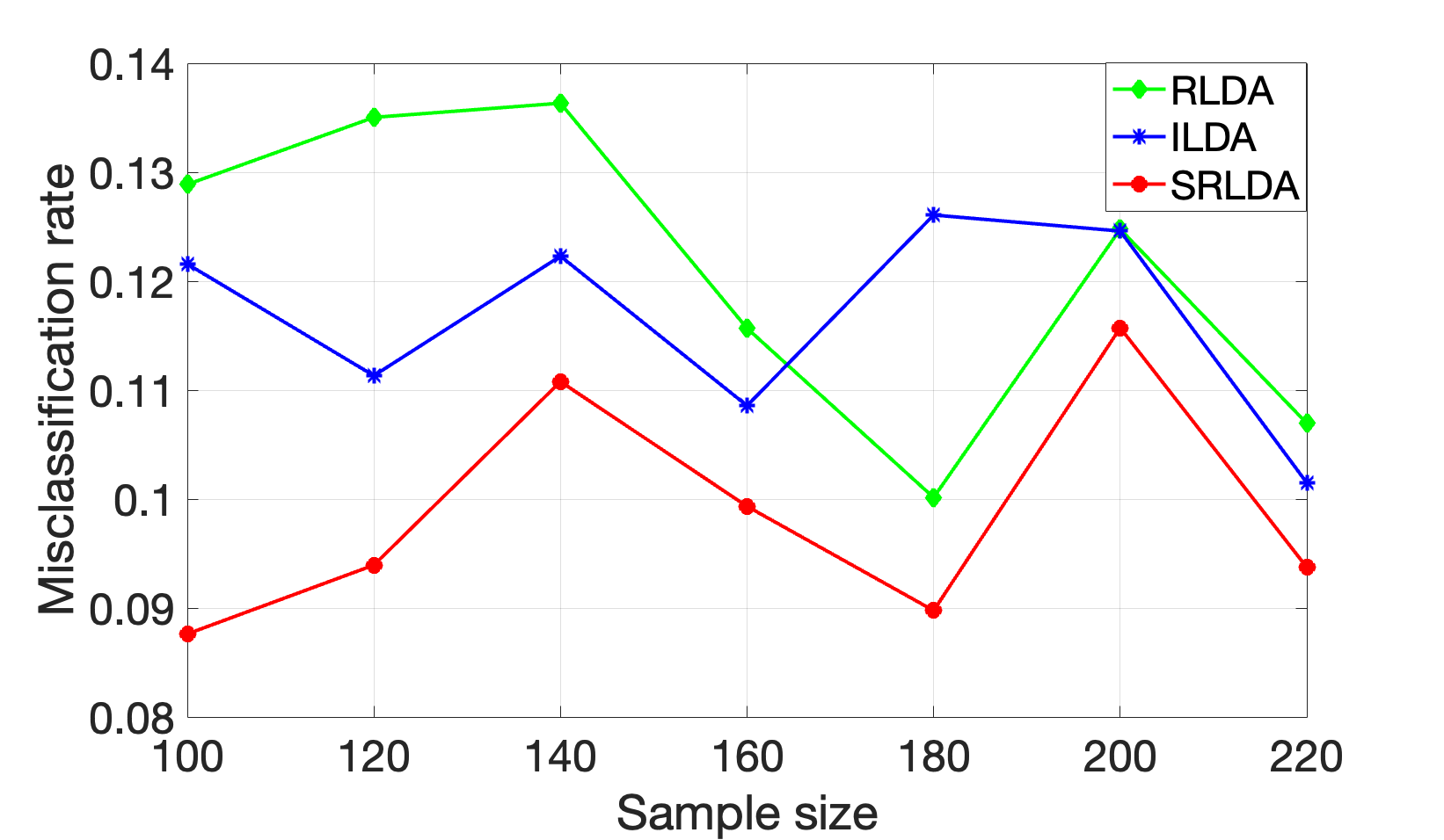
(a) $a=1$

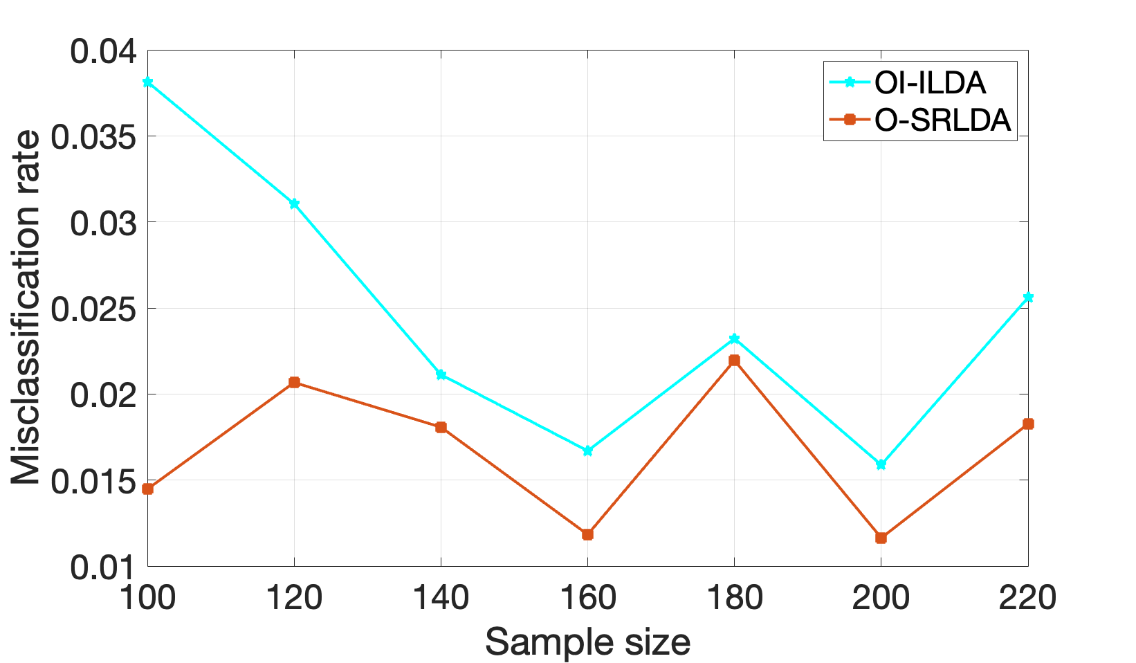
(b) $a=2$

Figure 1: Misclassification rate vs. sample size $n$ for $p=150$ and $\pi_{0}=0.2$. Comparison for RLDA, ILDA and SRLDA with simulated data.

			$a=1$						$a=2$
$n$			RLDA		ILDA		SRLDA		OI-ILDA		OI-SRLDA
100	mean		0.1289		0.1216		0.0876		0.0381		0.0145
	std.		0.0092		0.0698		0.0048		0.0569		0.0023
120	mean		0.1350		0.1113		0.0939		0.0310		0.0207
	std.		0.0124		0.0483		0.0034		0.0206		0.0018
140	mean		0.1363		0.1223		0.1180		0.0211		0.0181
	std.		0.0112		0.0389		0.0045		0.0159		0.0018
160	mean		0.1157		0.1086		0.0993		0.0167		0.0118
	std.		0.0087		0.0404		0.0028		0.0092		0.0015
180	mean		0.1001		0.1261		0.0898		0.0232		0.0219
	std.		0.0071		0.0713		0.0036		0.0043		0.0020
200	mean		0.1248		0.1246		0.1157		0.0159		0.0116
	std.		0.0066		0.0425		0.0023		0.0261		0.0017
220	mean		0.1069		0.1015		0.0937		0.0256		0.0183
	std.		0.0065		0.0349		0.0034		0.0212		0.0017

Table 1: The mean and standard variance of the misclassification rate of these five methods for scenario $a=1$ and scenario $a=2$.

5.2 Real Data

For empirical analysis, we use the “Wisconsin Diagnostic Breast Cancer (WDBS) Dataset” which is one of classic datasets and is publicly available at: WDBS. This data set includes 569 samples and 32 attributes which contain ID, diagnosis and 30 real-valued input features. Since the ID does not provide useful information for the actual analysis, we remove it. Diagnosis has two values: M and B, where M is malignant and B is benign, which can be considered class labels. The other 30 variables are determined by the mean values, standard deviations, and maximum values of each feature for 10 digitized nuclei features. The 10 basic characteristics are: radius (mean of distances from center to points on the perimeter), texture (standard deviation of gray-scale values), perimeter, area, smoothness (local variation in radius lengths), compactness, concavity (severity of concave portions of the contour), concave points (number of concave portions of the contour), symmetry, fractal dimension. During this empirical analysis, we apply the method proposed by [26] to determine the number of the spikes.

To compare the performance of the proposed classifiers SRLDA, OI-SRLDA with RLDA, I-LDA, OI-LDA, SVM and KNN. We use the following method for the real data set:

• Step 1: Let $q_{0}$ be the ratio between the total number of samples in class $\mathcal{C}_{0}$ to the total number of sample available in the full dataset. Denote by $n_{FULL}$ the total number of samples in the full dataset. Choose $n<n_{FULL}$ the number of training samples; set $n_{0}=\lfloor{q_{0}n}\rfloor$, where $\lfloor{\cdot}\rfloor$ is the floor function and $n_{1}=n-n_{0}$. Take $n_{i}$ training samples belonging to class $\mathcal{C}_{i}$ randomly from the full dataset. The remaining samples are used as a test dataset in order to estimate the misclassification rate.

• Step 2: Using the training dataset, design the SRLDA and OI-SRLDA classfier as explained in section 3 and the other six classifers.

• Step 3: Using the test dataset, estimate the true misclassification rate for eight calssifiers.

• Step 4: Repeat steps 1-4 500 times and determine the average misclassification rate of all classifiers.

The misclassification rates for different training sample size are presented in Table 2. As observed, the proposed classifier not only yields the best performance, but also has a much lower computational complexity than SVM and KNN.

	$n=200$	$n=250$	$n=300$	$n=350$	$n=400$	$n=450$
SRLDA	0.0516	0.0505	0.0489	0.0479	0.0472	0.0468
OI-SRLDA	0.0512	0.0500	0.0487	0.0473	0.0472	0.0465
OII-LDA	0.1951	0.1833	0.2148	0.2222	0.2011	0.2248
RLDA	0.0537	0.0513	0.0516	0.0496	0.0533	0.0534
SVM1	0.0694	0.0622	0.0594	0.0559	0.0548	0.0536
SVM2	0.0815	0.0726	0.0645	0.0606	0.0612	0.0593
SVM3	0.0638	0.0578	0.0545	0.0512	0.0516	0.0523
SVM4	0.3702	0.3684	0.3698	0.3674	0.3645	0.3674
KNN (k=1)	0.0573	0.0535	0.0538	0.0506	0.0524	0.0496
KNN (k=5)	0.0615	0.0566	0.0528	0.0492	0.0485	0.0460

Table 2: Comparison between the proposed classifier, R-LDA, SVM and KNN using WDBS dateset. Here SVM1, SVM2, SVM3, and SVM4 represent the SVM method with linear kernel, polynomial kernel (order=1), polynomial kernel (order=5), and gauss kernel respectively.

6 Conclusion

By using real data sets and simulated data sets for effective comparison, the SCRDA method has the following design points and outperformance.

• The original model design structure, that is spiked covariance model, is preserved as much as possible. By this way, the results of eigenvalue estimation and the limiting properties of the corresponding eigenvectors, under high-dimensional settings, are fully utilized.

• Regularization methods have once again demonstrated their important role in reducing risk, the misclassification rate.

• Based on the empirical analysis, the SRLDA method is quite competitive compared to SVM, KNN and other methods, but its algorithm is more lightweight and faster to calculate.

As a further extension, the same ideas can be extended to the other classification methods, such as quadratic discriminant classifier or other spiked covariance models.

Appendix A. Proof of Theorem 1

We introduce notation that will be used throughout the following proofs. Define ${\mathbf{G}}_{n}$

$${\mathbf{G}}_{n}={\mathbf{I}}_{n}-\left[\begin{array}[]{cc}\frac{{\mathbf{1}}_{n_{0}}{\mathbf{1}}_{n_{0}}^{T}}{n_{0}}&{\mathbf{0}}_{n_{0}\times n_{1}}\\ {\mathbf{0}}_{n_{1}\times n_{0}}&\frac{{\mathbf{1}}_{n_{1}}{\mathbf{1}}_{n_{1}}^{T}}{n_{1}}\end{array}\right].$$ (6.3)

The data matrix ${\mathbf{X}}_{n}$ is a $p\times(n_{0}+n_{1})$ matrix obtained by

$${\mathbf{X}}_{n}=\left[{\mathbf{x}}_{1},{\mathbf{x}}_{2},...,{\mathbf{x}}_{n}\right],$$ (6.4)

and we can write the pooled sample covariance matrix as

$${\mathbf{S}}=\frac{1}{n-2}\left({\mathbf{X}}_{n}{\mathbf{G}}_{n}{\mathbf{X}}_{n}^{T}\right).$$ (6.5)

Let ${\mathbf{Z}}_{n}=\left[{\mathbf{z}}_{1},{\mathbf{z}}_{2},...,{\mathbf{z}}_{n}\right]$ denotes a $p\times(n_{0}+n_{1})$ random matrix such that the random vectors ${\mathbf{z}}_{i}$ have the standard multivariate Gaussian distribution. We can rewrite the data matrix as

$${\mathbf{X}}_{n}=\left[{\bm{\mu}}_{0}{\mathbf{1}}_{n_{0}}^{T},{\bm{\mu}}_{1}{\mathbf{1}}_{n_{1}}^{T}\right]+{\bm{\Sigma}}^{1/2}{\mathbf{Z}}_{n}.$$ (6.6)

Note that

$$\left(\left[{\bm{\mu}}_{0}{\mathbf{1}}_{n_{0}}^{T},{\bm{\mu}}_{1}{\mathbf{1}}_{n_{1}}^{T}\right]+{\bm{\Sigma}}^{1/2}{\mathbf{Z}}_{n}\right){\mathbf{G}}_{n}={\bm{\Sigma}}^{1/2}{\mathbf{Z}}_{n}{\mathbf{G}}_{n}.$$ (6.7)

Using (6.3)-(6.7) one can write

$${\mathbf{S}}=\frac{1}{n-2}\left({\bm{\Sigma}}^{1/2}{\mathbf{Z}}_{n}{\mathbf{G}}_{n}{\mathbf{Z}}_{n}^{T}{\bm{\Sigma}}^{1/2}\right).$$ (6.8)

Consider the sequence of discrimination problems defined by (2.10). Now let

$${\mathbf{1}}_{n_{0}^{-1},n_{1}^{-1}}\overset{\Delta}{=}\left[{\mathbf{1}}_{n_{0}}^{T}/n_{0},{\mathbf{1}}_{n_{1}}^{T}/n_{1}\right]^{T},\,\,\,\,{\mathbf{1}}_{n_{0}^{-1},-n_{1}^{-1}}\overset{\Delta}{=}\left[{\mathbf{1}}_{n_{0}}^{T}/n_{0},-{\mathbf{1}}_{n_{1}}^{T}/n_{1}\right]^{T},$$

and ${\bm{\mu}}={\bm{\mu}}_{0}-{\bm{\mu}}_{1}$. Then

$$\overline{{\mathbf{x}}}_{0}+\overline{{\mathbf{x}}}_{1}={\mathbf{X}}_{n}{\mathbf{1}}_{n_{0}^{-1},n_{1}^{-1}}={\bm{\mu}}_{0}+{\bm{\mu}}_{1}+{\bm{\Sigma}}^{1/2}{\mathbf{Z}}_{n}{\mathbf{1}}_{n_{0}^{-1},n_{1}^{-1}}$$

and

$$\overline{{\mathbf{x}}}_{0}-\overline{{\mathbf{x}}}_{1}={\mathbf{X}}_{n}{\mathbf{1}}_{n_{0}^{-1},-n_{1}^{-1}}={\bm{\mu}}+{\bm{\Sigma}}^{1/2}{\mathbf{Z}}_{n}{\mathbf{1}}_{n_{0}^{-1},-n_{1}^{-1}}.$$ (6.9)

By Kolmogorov Law of Large Numbers, we have $\left\|{\mathbf{Z}}_{n}{\mathbf{1}}_{n_{0}^{-1},-n_{1}^{-1}}\right\|^{2}\xrightarrow{a.s.}J_{1}+J_{2}$ and $\left\|{\mathbf{Z}}_{n}{\mathbf{1}}_{n_{0}^{-1},n_{1}^{-1}}\right\|^{2}\xrightarrow{a.s.}J_{1}+J_{2}$. Therefore, under Assumption 3.1 to 3.4, it is natural that $\left\|\overline{{\mathbf{x}}}_{0}+\overline{{\mathbf{x}}}_{1}\right\|=O_{a.s.}(1)$ and $\left\|\overline{{\mathbf{x}}}_{0}-\overline{{\mathbf{x}}}_{1}\right\|=O_{a.s.}(1)$. Then $\exists K>0$, $\forall(\gamma_{1},\gamma_{2})\in{\mathbb{A}}$, such that

$$G\left({\bm{\mu}}_{i},\overline{{\mathbf{x}}}_{0},\overline{{\mathbf{x}}}_{1},{\widetilde{\mathbf{H}}}\right)=O_{a.s.}(1),\;\;\;\;0<K\delta\overset{a.s.}{\leq}D\left(\overline{{\mathbf{x}}}_{0},\overline{{\mathbf{x}}}_{1},{\widetilde{\mathbf{H}}},\Sigma\right)=O_{a.s.}(1)$$ (6.10)

uniformly. Using (6.6), rewrite

$$G\left({\bm{\mu}}_{i},\overline{{\mathbf{x}}}_{0},\overline{{\mathbf{x}}}_{1},{\widetilde{\mathbf{H}}}\right) = \frac{(-1)^{i}}{2}{\bm{\mu}}^{T}{\widetilde{\mathbf{H}}}{\bm{\mu}}-\frac{1}{2}\left({\bm{\Sigma}}^{1/2}{\mathbf{Z}}_{n}{\mathbf{1}}_{n_{0}^{-1},n_{1}^{-1}}\right)^{T}{\widetilde{\mathbf{H}}}\left({\bm{\Sigma}}^{1/2}{\mathbf{Z}}_{n}{\mathbf{1}}_{n_{0}^{-1},-n_{1}^{-1}}\right)$$

$$+\frac{(-1)^{i}}{2}{\bm{\mu}}^{T}{\widetilde{\mathbf{H}}}{\bm{\Sigma}}^{1/2}{\mathbf{Z}}_{n}{\mathbf{1}}_{n_{0}^{-1},-n_{1}^{-1}}-\frac{1}{2}\left({\bm{\Sigma}}^{1/2}{\mathbf{Z}}_{n}{\mathbf{1}}_{n_{0}^{-1},n_{1}^{-1}}\right)^{T}{\widetilde{\mathbf{H}}}{\bm{\mu}},$$

$$D\left(\overline{{\mathbf{x}}}_{0},\overline{{\mathbf{x}}}_{1},{\widetilde{\mathbf{H}}},\Sigma\right) = {\bm{\mu}}^{T}{\widetilde{\mathbf{H}}}{\bm{\Sigma}}{\widetilde{\mathbf{H}}}{\bm{\mu}}+2{\bm{\mu}}^{T}{\widetilde{\mathbf{H}}}{\bm{\Sigma}}{\widetilde{\mathbf{H}}}{\bm{\Sigma}}^{1/2}{\mathbf{Z}}_{n}{\mathbf{1}}_{n_{0}^{-1},-n_{1}^{-1}}$$

$$+{\rm tr}\left({\widetilde{\mathbf{H}}}{\bm{\Sigma}}{\widetilde{\mathbf{H}}}{\bm{\Sigma}}^{1/2}{\mathbf{Z}}_{n}{\mathbf{1}}_{n_{0}^{-1},-n_{1}^{-1}}{\mathbf{1}}_{n_{0}^{-1},-n_{1}^{-1}}^{T}{\mathbf{Z}}_{n}^{T}{\bm{\Sigma}}^{1/2}\right).$$

According the Theorem (Couillet and Debbah, 2011, Theorem 3.4 and 3.7) in [9], we have

$$\left({\bm{\mu}}^{T}{\widetilde{\mathbf{H}}}{\bm{\Sigma}}^{1/2}{\mathbf{Z}}_{n}{\mathbf{1}}_{n_{0}^{-1},-n_{1}^{-1}}\right)^{2} \xrightarrow{a.s.} 0,$$ (6.11)

$${\bm{\mu}}^{T}{\widetilde{\mathbf{H}}}{\bm{\Sigma}}^{1/2}{\mathbf{Z}}_{n}{\mathbf{1}}_{n_{0}^{-1},-n_{1}^{-1}} \xrightarrow{a.s.} 0,$$

$${\mathbf{1}}_{n_{0}^{-1},n_{1}^{-1}}^{T}{\mathbf{Z}}_{n}^{T}{\bm{\Sigma}}^{1/2}{\widetilde{\mathbf{H}}}{\bm{\mu}} \xrightarrow{a.s.} 0.$$

Then

$$G\left({\bm{\mu}}_{i},\overline{{\mathbf{x}}}_{0},\overline{{\mathbf{x}}}_{1},{\widetilde{\mathbf{H}}}\right) \xrightarrow{a.s.} \frac{(-1)^{i}}{2}{\bm{\mu}}^{T}{\widetilde{\mathbf{H}}}{\bm{\mu}}-\frac{1}{2}\left({\bm{\Sigma}}^{1/2}{\mathbf{Z}}_{n}{\mathbf{1}}_{n_{0}^{-1},n_{1}^{-1}}\right)^{T}{\widetilde{\mathbf{H}}}\left({\bm{\Sigma}}^{1/2}{\mathbf{Z}}_{n}{\mathbf{1}}_{n_{0}^{-1},-n_{1}^{-1}}\right),$$

$$D\left(\overline{{\mathbf{x}}}_{0},\overline{{\mathbf{x}}}_{1},{\widetilde{\mathbf{H}}},\Sigma\right) \xrightarrow{a.s.} {\bm{\mu}}^{T}{\widetilde{\mathbf{H}}}{\bm{\Sigma}}{\widetilde{\mathbf{H}}}{\bm{\mu}}+\left(n_{0}^{-1}+n_{1}^{-1}\right){\rm tr}\left({\widetilde{\mathbf{H}}}{\bm{\Sigma}}{\widetilde{\mathbf{H}}}{\bm{\Sigma}}\right).$$ (6.13)

It is well-known that in the Gaussian case the sample mean $\overline{{\mathbf{x}}}_{i}$, is independent from ${\mathbf{S}}_{i}$, $i=0,1$. Therefore, ${\mathbf{Z}}_{n}{\mathbf{1}}_{n_{0}^{-1},n_{1}^{-1}}$ and ${\mathbf{Z}}_{n}{\mathbf{1}}_{n_{0}^{-1},-n_{1}^{-1}}$ are independent of ${\widetilde{\mathbf{H}}}$.

For first element of (Appendix A. Proof of Theorem 1), according (3.9), we have

$${\bm{\mu}}^{T}{\widetilde{\mathbf{H}}}{\bm{\mu}} = \left\|{\bm{\mu}}\right\|^{2}-\sum_{j\in{\mathbb{I}}_{1}}\gamma_{1,j}\left({\bm{\mu}}^{T}{\mathbf{u}}_{j}\right)^{2}-\sum_{j\in{\mathbb{I}}_{2}}\gamma_{2,j}\left({\bm{\mu}}^{T}{\mathbf{u}}_{j}\right)^{2}$$

$$\xrightarrow{a.s.} \|{\bm{\mu}}\|^{2}\left(1-\sum_{j\in{\mathbb{I}}_{1}}\gamma_{1,j}a_{j}b_{j}-\sum_{j\in{\mathbb{I}}_{2}}\gamma_{2,j}a_{j}b_{j}\right)$$

$$\triangleq \|{\bm{\mu}}\|^{2}\overline{G}\left(\gamma_{1},\gamma_{2}\right),$$

where $a_{j}=\frac{\lambda_{j}^{2}-c}{\lambda_{j}(\lambda_{j}+c)}$ and $b_{j}=\frac{\left({\bm{\mu}}^{T}{\mathbf{v}}_{j}\right)^{2}}{\|{\bm{\mu}}\|^{2}}$ for $j={\mathbb{I}}$. For the second one of (Appendix A. Proof of Theorem 1), we have ${\mathbf{1}}_{n_{0}}^{T}{\mathbf{Z}}_{n_{0}}^{T}{\bm{\Sigma}}^{1/2}\widetilde{{\mathbf{H}}}{\bm{\Sigma}}^{1/2}{\mathbf{Z}}_{n_{1}}{\mathbf{1}}_{n_{1}}\xrightarrow{a.s.}0$, which is the same as (6.11). And then it is deduced that

$$\left({\bm{\Sigma}}^{1/2}{\mathbf{Z}}_{n}{\mathbf{1}}_{n_{0}^{-1},n_{1}^{-1}}\right)^{T}{\widetilde{\mathbf{H}}}\left({\bm{\Sigma}}^{1/2}{\mathbf{Z}}_{n}{\mathbf{1}}_{n_{0}^{-1},-n_{1}^{-1}}\right)$$

$$\xrightarrow{a.s.} {\mathbf{1}}_{n_{0}}^{T}{\mathbf{Z}}_{n_{0}}^{T}{\bm{\Sigma}}^{1/2}\widetilde{{\mathbf{H}}}{\bm{\Sigma}}^{1/2}{\mathbf{Z}}_{n_{0}}{\mathbf{1}}_{n_{0}}-{\mathbf{1}}_{n_{1}}^{T}{\mathbf{Z}}_{n_{1}}^{T}{\bm{\Sigma}}^{1/2}\widetilde{{\mathbf{H}}}{\bm{\Sigma}}^{1/2}{\mathbf{Z}}_{n_{1}}{\mathbf{1}}_{n_{1}}$$

$$\xrightarrow{a.s.} \left(n_{0}^{-1}-n_{1}^{-1}\right){\rm tr}\left(\left({\mathbf{I}}_{p}-\sum_{j\in{\mathbb{I}}_{1}}\gamma_{1,j}{\mathbf{u}}_{j}{\mathbf{u}}_{j}^{T}-\sum_{j\in{\mathbb{I}}_{2}}\gamma_{2,j}{\mathbf{u}}_{j}{\mathbf{u}}_{j}^{T}\right){\bm{\Sigma}}\right)$$

$$\xrightarrow{a.s.} \sigma^{2}\left(J_{0}-J_{1}\right).$$

in which ${\mathbf{Z}}_{n}=\left[{\mathbf{Z}}_{n_{0}},{\mathbf{Z}}_{n_{1}}\right]$. Similarly, for (6.13), we have $\left(n_{0}^{-1}+n_{1}^{-1}\right){\rm tr}\left({\widetilde{\mathbf{H}}}{\bm{\Sigma}}{\widetilde{\mathbf{H}}}{\bm{\Sigma}}\right)\xrightarrow{a.s.}\sigma^{4}\left(J_{0}+J_{1}\right)$, and

$${\bm{\mu}}^{T}{\widetilde{\mathbf{H}}}{\bm{\Sigma}}{\widetilde{\mathbf{H}}}{\bm{\mu}} = \sigma^{2}\left({\bm{\mu}}^{T}{\widetilde{\mathbf{H}}}^{2}{\bm{\mu}}+\sum_{j\in{\mathbb{I}}_{1}}\lambda_{j}\left({\bm{\mu}}^{T}{\widetilde{\mathbf{H}}}{\mathbf{v}}_{j}\right)^{2}+\sum_{j\in{\mathbb{I}}_{2}}\lambda_{j}\left({\bm{\mu}}^{T}{\widetilde{\mathbf{H}}}{\mathbf{v}}_{j}\right)^{2}\right)$$

$$\xrightarrow{a.s.} \sigma^{2}\|{\bm{\mu}}\|^{2}\left(\begin{array}[]{l}1+\sum_{j\in{\mathbb{I}}_{1}}\lambda_{j}b_{j}+\sum_{j\in{\mathbb{I}}_{2}}\lambda_{j}b_{j}\\ -2\sum_{j\in{\mathbb{I}}_{1}}(1+\lambda_{j})a_{j}b_{j}\gamma_{1,j}-2\sum_{j\in{\mathbb{I}}_{2}}(1+\lambda_{j})a_{j}b_{j}\gamma_{2,j}\\ +\sum_{j\in{\mathbb{I}}_{1}}a_{j}b_{j}\left(1+\lambda_{j}a_{j}\right)\gamma_{1,j}^{2}+\sum_{j\in{\mathbb{I}}_{2}}a_{j}b_{j}\left(1+\lambda_{j}a_{j}\right)\gamma_{2,j}^{2}\end{array}\right)$$

$$\triangleq \sigma^{2}\|{\bm{\mu}}\|^{2}\overline{D}(\gamma_{1},\gamma_{2}),$$

in which

$$\frac{{\bm{\mu}}^{T}{\widetilde{\mathbf{H}}}^{2}{\bm{\mu}}}{\|{\bm{\mu}}\|^{2}} \xrightarrow{a.s.} 1+\sum_{j\in{\mathbb{I}}_{1}}\left(\gamma_{1,j}^{2}-2\gamma_{1,j}\right)a_{j}b_{j}+\sum_{j\in{\mathbb{I}}_{2}}\left(\gamma_{2,j}^{2}-2\gamma_{2,j}\right)a_{j}b_{j},$$

$$\frac{|{\bm{\mu}}^{T}{\widetilde{\mathbf{H}}}{\mathbf{v}}_{j}|}{\|{\bm{\mu}}\|} \xrightarrow{a.s.} \sqrt{b_{j}\left(1-2\gamma_{i,j}a_{j}+\gamma_{i,j}^{2}a_{j}^{2}\right)},$$

with $j={\mathbb{I}}_{1}$ for $i=1$ or $j={\mathbb{I}}_{2}$ for $i=2$.

Now we prove (3.2) and (3.3) hold uniformly for any ${\bm{\gamma}}=\left(\gamma_{1},\gamma_{2}\right)\in{\mathbb{A}}$. According the structure of set ${\mathbb{A}}$, we have

• $\gamma_{1,j}=\frac{\gamma_{1}\lambda_{j}}{1+\gamma_{1}\lambda_{j}}$ ($j\in{\mathbb{I}}_{1}$) and $\gamma_{2,k}=\frac{\gamma_{2}\lambda_{k}}{1+\gamma_{2}\lambda_{k}}$ ($j\in{\mathbb{I}}_{2}$) are uniformly continuous on the closed set $\overline{{\mathbb{A}}}$.

• for any $\varepsilon>0$, there exist a finite number of ${\bm{\gamma}}_{1},...,{\bm{\gamma}}_{m}$, such that $\overline{{\mathbb{A}}}\subset\cup_{t=1}^{m}U\left({\bm{\gamma}}_{t},\varepsilon\right)$ and $\cup_{t=1}^{m}U\left({\bm{\gamma}}_{t},\varepsilon\right)\bigcap{\mathbb{I}}_{2}=\emptyset$.

Rewrite ${\bf G}_{i}({\bm{\gamma}})=G\left({\bm{\mu}}_{i},\overline{{\mathbf{x}}}_{0},\overline{{\mathbf{x}}}_{1},{\widetilde{\mathbf{H}}}\right)$, ${\bf D}_{i}({\bm{\gamma}})=D\left(\overline{{\mathbf{x}}}_{0},\overline{{\mathbf{x}}}_{1},{\widetilde{\mathbf{H}}},\Sigma\right)$,

$$\overline{{\bf G}}_{i}({\bm{\gamma}})=\frac{(-1)^{i}}{2}\|{\bm{\mu}}\|^{2}\overline{G}\left(\gamma_{1},\gamma_{2}\right)+\sigma^{2}\left(J_{0}-J_{1}\right),$$

$$\overline{{\bf D}}_{i}({\bm{\gamma}})={\bm{\mu}}^{T}{\widetilde{\mathbf{H}}}{\bm{\Sigma}}{\widetilde{\mathbf{H}}}{\bm{\mu}}+\left(n_{0}^{-1}+n_{1}^{-1}\right){\rm tr}\left({\widetilde{\mathbf{H}}}{\bm{\Sigma}}{\widetilde{\mathbf{H}}}{\bm{\Sigma}}\right).$$

According to (6.10), $\forall{\bm{\gamma}}\in{\mathbb{A}}$, $\exists t\in\{1,...,m\}$, such that ${\bm{\gamma}}\in U\left({\bm{\gamma}}_{t},\varepsilon\right)$ and

$$\max\left\{\left|{{\bf G}}_{i}({\bm{\gamma}})-{{\bf G}}_{i}({\bm{\gamma}}_{t})\right|,\left|\overline{{\bf G}}_{i}({\bm{\gamma}}_{t})-\overline{{\bf G}}_{i}({\bm{\gamma}})\right|\right\} \overset{a.s.}{\leq} K_{1}\varepsilon,$$

$$\max\left\{\left|{{\bf D}}_{i}({\bm{\gamma}})-{{\bf D}}_{i}({\bm{\gamma}}_{t})\right|,\left|\overline{{\bf D}}_{i}({\bm{\gamma}}_{t})-\overline{{\bf D}}_{i}({\bm{\gamma}})\right|\right\} \overset{a.s.}{\leq} K_{2}\varepsilon.$$

Then, for any ${\bm{\gamma}}\in{\mathbb{A}}$,

$$\left|{{\bf G}}_{i}({\bm{\gamma}})-\overline{{\bf G}}_{i}({\bm{\gamma}})\right| {\leq} \left|{{\bf G}}_{i}({\bm{\gamma}})-{{\bf G}}_{i}({\bm{\gamma}}_{t})\right|+\left|{{\bf G}}_{i}({\bm{\gamma}}_{t})-\overline{{\bf G}}_{i}({\bm{\gamma}}_{t})\right|+\left|\overline{{\bf G}}_{i}({\bm{\gamma}}_{t})-\overline{{\bf G}}_{i}({\bm{\gamma}})\right|$$

$$\overset{a.s.}{\leq} 2K_{1}\varepsilon+\max_{t=1,...,m}\left|{{\bf G}}_{i}({\bm{\gamma}}_{t})-\overline{{\bf G}}_{i}({\bm{\gamma}}_{t})\right|=2K_{1}\varepsilon+o_{a.s.}(1),$$

$$\left|{{\bf D}}_{i}({\bm{\gamma}})-\overline{{\bf D}}_{i}({\bm{\gamma}})\right| {\leq} \left|{{\bf D}}_{i}({\bm{\gamma}})-{{\bf D}}_{i}({\bm{\gamma}}_{t})\right|+\left|{{\bf D}}_{i}({\bm{\gamma}}_{t})-\overline{{\bf D}}_{i}({\bm{\gamma}}_{t})\right|+\left|\overline{{\bf D}}_{i}({\bm{\gamma}}_{t})-\overline{{\bf D}}_{i}({\bm{\gamma}})\right|$$

$$\overset{a.s.}{\leq} 2K_{2}\varepsilon+\max_{t=1,...,m}\left|{{\bf D}}_{i}({\bm{\gamma}}_{t})-\overline{{\bf D}}_{i}({\bm{\gamma}}_{t})\right|=2K_{2}\varepsilon+o_{a.s.}(1),$$

uniformly. Then (3.2) and (3.3) hold uniformly.

Appendix B. Proof of Theorem 3

Let $\omega_{i}=\gamma_{i,1}\in(0,1)$ for $i=1,2$. Then, $\gamma_{1}$ and $\gamma_{2}$ can be rewritten as

$$\gamma_{1}=\frac{\omega_{1}}{(1-\omega_{1})\lambda_{1}},\;\;\mbox{and}\;\;\gamma_{2}=\frac{-\omega_{2}}{(1-\omega_{2})\lambda_{-1}}.$$

Further,

$$\gamma_{1,j} = \frac{\omega_{1}\lambda_{j}}{(1-\omega_{1})\lambda_{1}+\omega_{1}\lambda_{j}},\;\;\;j\in{\mathbb{I}}_{1},$$ (6.15)

$$\gamma_{2,j} = \frac{-\omega_{2}\lambda_{j}}{(1-\omega_{2})\lambda_{-1}-\omega_{2}\lambda_{j}},\;\;\;j\in{\mathbb{I}}_{2}.$$ (6.16)

Plugging (6.15) and (6.16) into (3.4) and (3.5), we have

$$\widetilde{G}(\omega_{1},\omega_{2})=\overline{G}(\gamma_{1},\gamma_{2})\;\;\mbox{and}\;\;\widetilde{D}(\omega_{1},\omega_{2})=\overline{D}(\gamma_{1},\gamma_{2}).$$

where

$$f_{0}(\omega_{1},\omega_{2})=\frac{\widetilde{G}(\omega_{1},\omega_{2})-\eta}{\sqrt{\widetilde{D}(\omega_{1},\omega_{2})+\zeta}},\;\;\;\;f_{1}(\omega_{1},\omega_{2})=\frac{\widetilde{G}(\omega_{1},\omega_{2})+\eta}{\sqrt{\widetilde{D}(\omega_{1},\omega_{2})+\zeta}}.$$

Thus, the objective function can be written as

$$f(\omega_{1},\omega_{2})=\pi_{0}\Phi\left(-\frac{1}{2\sqrt{\alpha}}f_{0}(\omega_{1},\omega_{2})\right)+\pi_{1}\Phi\left(-\frac{1}{2\sqrt{\alpha}}f_{1}(\omega_{1},\omega_{2})\right)$$

Thus, (3.1) is equivalent to

$$\omega_{1}^{*},\omega_{2}^{*}=\mathop{\arg\min}\limits_{\omega_{1},\omega_{2}\in(0,1)}f(\omega_{1},\omega_{2})$$

by which

$$\gamma_{1}^{*}=\frac{\omega_{1}^{*}}{(1-\omega_{1}^{*})\lambda_{1}},\;\;\mbox{and}\;\;\gamma_{2}^{*}=\frac{-\omega_{2}^{*}}{(1-\omega_{2}^{*})\lambda_{-1}}.$$

Appendix C. Proof of Theorem 5

We will assume without loss of generality that $\pi_{1}>\pi_{0}$. Using the notations of Appendix B, we have $\omega_{i}=\gamma_{i,1}\in(0,1)$ for $i=1,2$, and $\gamma_{1}=\frac{\omega_{1}}{(1-\omega_{1})\lambda_{1}}$, $\gamma_{2}=\frac{-\omega_{2}}{(1-\omega_{2})\lambda_{-1}}$,

$$\widetilde{G}(\omega_{1},\omega_{2})=\overline{G}(\gamma_{1},\gamma_{2}),\;\;\;\;\widetilde{D}(\omega_{1},\omega_{2})=\overline{D}(\gamma_{1},\gamma_{2}).$$

Let $R=\frac{\widetilde{G}(\gamma_{1},\gamma_{2})}{\sqrt{\widetilde{D}(\gamma_{1},\gamma_{2})+\zeta}}$, the objective function (4.1) can be written as

$$f(\omega_{1},\omega_{2})=\pi_{0}\Phi\left(\frac{-R}{2\sqrt{\alpha}}+\frac{\sqrt{\alpha}}{R}\log\frac{\pi_{1}}{\pi_{0}}\right)+\pi_{1}\Phi\left(\frac{-R}{2\sqrt{\alpha}}-\frac{\sqrt{\alpha}}{R}\log\frac{\pi_{1}}{\pi_{0}}\right)$$ (6.17)

Thus,

$$\gamma_{1}^{*},\gamma_{2}^{*}=\mathop{\arg\min}\limits_{\gamma_{1},\gamma_{2}>0}\overline{\varepsilon}^{OI-SRLDA}(\gamma_{1},\gamma_{2})$$

is equivalent to

$$\omega_{1}^{*},\omega_{2}^{*}=\mathop{\arg\min}\limits_{\omega_{1},\omega_{2}\in(0,1)}f(\omega_{1},\omega_{2}).$$

by which

$$\gamma_{1}^{*}=\frac{\omega_{1}^{*}}{(1-\omega_{1}^{*})\lambda_{1}},\;\;\mbox{and}\;\;\gamma_{2}^{*}=\frac{-\omega_{2}^{*}}{(1-\omega_{2}^{*})\lambda_{-1}}.$$

Appendix D. Proof of Theorem 4

Recall(2.1). Without loss of generality, rewrite ${\bm{\Sigma}}$ as

$${\bm{\Sigma}}={\mathbf{I}}_{p}+{\mathbf{V}}{\rm diag}(\lambda_{1},\cdots,\lambda_{r_{1}},0,\cdots,0,\lambda_{-r_{2}},\cdots,\lambda_{-1}){\mathbf{V}}^{T},$$

in which ${\mathbf{V}}=({\mathbf{v}}_{1},\cdots,{\mathbf{v}}_{r_{1}},{\mathbf{v}}_{r_{1}+1},\cdots,{\mathbf{v}}_{p-r_{2}},{\mathbf{v}}_{-r_{2}},\cdots,{\mathbf{v}}_{-1})$ and is an unit orthogonal matrix. Therefore, we have

$${\bm{\Sigma}}^{-1}={\mathbf{I}}_{p}-{\mathbf{V}}{\mathbf{D}}{\mathbf{V}}^{T},$$

with

$${\mathbf{D}}={\rm diag}\left(\dfrac{\lambda_{1}}{1+\lambda_{1}},\cdots,\dfrac{\lambda_{r_{1}}}{1+\lambda_{r_{1}}},0,\cdots,0,\dfrac{\lambda_{-r_{2}}}{1+\lambda_{-r_{2}}},\cdots,\dfrac{\lambda_{-1}}{1+\lambda_{-1}}\right).$$

Baik and Silverstein [3] proves that for each $i\in{\mathbb{I}}$,

$$l_{i}\xrightarrow{a.s.}\theta(\lambda_{i}).$$ (6.18)

Here $\theta(z)=1+z+J+{J}/{z}$ with $z\in\mathbb{C}$. Let $\Gamma_{i}(:=\{z:|z-\lambda_{i}|\leq\rho_{i},z\in{\mathbb{C}}\})$ be the boundary of a disc centered at $\lambda_{i}$ with radius $\rho_{i}$,

$$\rho_{i}:=\dfrac{1}{2}\left(\underset{j\neq i}{\min}\left|\lambda_{i}-\lambda_{j}\right|\land\left|\lambda_{i}-\sqrt{J}\right|\land\left|\lambda_{i}+\sqrt{J}\right|\right),$$ (6.19)

such that the disc is away from the critical value $\sqrt{J}$ and other $\lambda_{j}$’s. Therefore under the definitions of $\rho_{i}$ and $\theta(z)$, the contour $\theta(\Gamma_{i})$ encloses exactly the $i$-th eigenvalue of ${\mathbf{S}}$, i.e. $l_{i},i\in{\mathbb{I}}$. According to (6.18), together with the Cauchy integral, we have the following equality

$$\left\langle{\mathbf{w}},{\mathbf{u}}_{i}{\mathbf{u}}_{i}^{T}{\mathbf{w}}\right\rangle\overset{a.s.}{=}-\dfrac{1}{2\pi i}\oint_{\theta(\Gamma_{i})}{\mathbf{w}}^{T}{\mathbf{G}}(z){\mathbf{w}}\ {\rm{d}}z,$$ (6.20)

where ${\mathbf{G}}(z)=\left({\mathbf{S}}-z{\mathbf{I}}_{p}\right)^{-1}$ and ${\mathbf{S}}$ is given in (6.8). Since ${\mathbf{S}}$ has the same distribution as that of ${\mathbf{S}}^{\prime}=\frac{1}{n-2}\left({\bm{\Sigma}}^{1/2}{\mathbf{Z}}_{n-2}{\mathbf{Z}}_{n-2}^{T}{\bm{\Sigma}}^{1/2}\right)$ where ${\mathbf{Z}}_{(\cdot)}$ has the same definition as that of (6.6), rewrite ${\mathbf{S}}$ as ${\mathbf{S}}^{\prime}$. Then

$${\mathbf{G}}(z)={\bm{\Sigma}}^{-\frac{1}{2}}\left(\mathcal{G}^{-1}(z)+z{\mathbf{V}}{\mathbf{D}}{\mathbf{V}}^{T}\right)^{-1}{\bm{\Sigma}}^{-\frac{1}{2}},$$

where $\mathcal{G}(z)=\left(\frac{1}{n-2}{\mathbf{Z}}_{n-2}{\mathbf{Z}}_{n-2}^{T}-z{\mathbf{I}}_{p}\right)^{-1}$, of which the spectral distribution converges to $m(z)=\int(x-z)^{-1}{\rm d}F(x)$, with $F(x)$ being the distribution of MP-law [35]. Then, it is follows from the matrix inversion lemma that

$${\mathbf{w}}^{T}{\mathbf{G}}(z){\mathbf{w}}=\widetilde{{\mathbf{w}}}^{T}\mathcal{G}(z)\widetilde{{\mathbf{w}}}-z\widetilde{{\mathbf{w}}}^{T}\mathcal{G}(z){\mathbf{V}}\overline{{\bf G}}(z){\mathbf{V}}^{T}\mathcal{G}(z)\widetilde{{\mathbf{w}}},$$ (6.21)

in which $\widetilde{{\mathbf{w}}}=\Sigma^{-1/2}{\mathbf{w}}$ and $\overline{{\bf G}}(z)=\left({\mathbf{D}}^{-1}+z{\mathbf{V}}^{T}\mathcal{G}(z){\mathbf{V}}\right)^{-1}$. Plugging (6.21) into (6.20), since $\theta(\lambda_{i})$ is not a singularity of $\mathcal{G}(z)$, so the contour integral of $\widetilde{{\mathbf{w}}}^{T}\mathcal{G}(z)\widetilde{{\mathbf{w}}}$ on $\theta(\Gamma_{i})$ is zero almost surely, one has

$$\left\langle{\mathbf{w}},{\mathbf{u}}_{i}{\mathbf{u}}_{i}^{T}{\mathbf{w}}\right\rangle\overset{a.s.}{=}\dfrac{1}{2\pi i}\oint_{\theta(\Gamma_{i})}z\widetilde{{\mathbf{w}}}^{T}\mathcal{G}(z){\mathbf{V}}\overline{{\bf G}}(z){\mathbf{V}}^{T}\mathcal{G}(z)\widetilde{{\mathbf{w}}}\ {\rm{d}}z.$$ (6.22)

Rewrite $\mathcal{G}(z)=\mathcal{G}(z)-m(z)I_{p}+m(z)I_{p}:=\Xi(z)+m(z)I_{p}$. Then for the integrand, we have

$$\begin{aligned} \overline{{\bf G}}(z)={\mathbf{L}}(z)-z\overline{{\bf G}}(z){\mathbf{V}}^{T}\Xi(z){\mathbf{V}}{\mathbf{L}}(z),\end{aligned}$$ (6.23)

where ${\mathbf{L}}(z):=\left({\mathbf{D}}^{-1}+zm(z){\mathbf{I}}_{p}\right)^{-1}$. With (6.23), we can further rewrite (6.22) as

$$\begin{aligned} &\left\langle{\mathbf{w}},{\mathbf{u}}_{i}{\mathbf{u}}_{i}^{T}{\mathbf{w}}\right\rangle\\ =&\dfrac{1}{2\pi i}\oint_{\theta(\Gamma_{i})}z\Delta^{T}\left({\mathbf{L}}(z)-z\overline{{\bf G}}(z){\mathbf{V}}^{T}\Xi(z){\mathbf{V}}{\mathbf{L}}(z)\right)\Delta\ {\rm{d}}z,\end{aligned}$$ (6.24)

where $\Delta:=\left(m(z){\mathbf{V}}^{T}\widetilde{{\mathbf{w}}}+{\mathbf{V}}^{T}\Xi(z)\widetilde{{\mathbf{w}}}\right)$. According to Theorem 2.4 in [1], we have

$$\left\|\widetilde{{\mathbf{w}}}^{T}\Xi(z){\mathbf{V}}\right\|\prec O\left(N^{-1/2}\right),\,\,\,\,\,\,\left\|{\mathbf{V}}^{T}\Xi(z){\mathbf{V}}\right\|\prec O\left(N^{-1/2}\right)$$

uniformly for any $z\in\theta(\Gamma_{i})$ in which $\xi(z)\prec\zeta(z)$ means $\xi$ is stochastically dominated by $\zeta$, uniformly in $z$. According Definition 2.1 and Remark 2.6 of [1], it is uniformed for $z\in\theta(\Gamma_{i})$ that

$$\left\|\widetilde{{\mathbf{w}}}^{T}\Xi(z){\mathbf{V}}\right\|\xrightarrow{a.s.}0,\,\,\,\,\,\,\left\|{\mathbf{V}}^{T}\Xi(z){\mathbf{V}}\right\|\xrightarrow{a.s.}0.$$ (6.25)

By variable substitution method, for $z\in\Gamma_{i}$, ${\mathbf{V}}{\mathbf{L}}(\theta(z)){\mathbf{V}}^{T}$ is rewriten as

$$\sum_{j\in{\mathbb{I}}}\dfrac{{\mathbf{v}}_{j}{\mathbf{v}}^{T}_{j}}{1+\lambda_{j}^{-1}+\theta(z)m(\theta(z))}=\sum_{j\in{\mathbb{I}}}\dfrac{z\lambda_{j}{\mathbf{v}}_{j}{\mathbf{v}}^{T}_{j}}{z-\lambda_{j}}$$ (6.26)

under the fact $1+z^{-1}+\theta(z)m(\theta(z))=0$. We have $\sup_{z\in\theta{(\Gamma_{i}})}\|L(z)\|_{\rm op}$ is bounded. Further,

$$\left\|\left({\mathbf{D}}^{-1}+\theta(z){\mathbf{V}}^{T}\mathcal{G}(\theta(z)){\mathbf{V}}\right)^{-1}\right\|_{\rm op}$$ (6.27)

$$\leq \dfrac{M_{1}}{\min_{j\in{\mathbb{I}}}\frac{\lambda_{j}}{1+\lambda_{j}}+\min\left\{\left|\theta(z)-(1+\sqrt{J})^{2}\right|,\left|\theta(z)-(1-\sqrt{J})^{2}\right|\right\}}\leq M$$

for any $z\in\Gamma_{i}$. From 6.24 to 6.27, we have

$$\left\langle{\mathbf{w}},{\mathbf{u}}_{i}{\mathbf{u}}_{i}^{T}{\mathbf{w}}\right\rangle\overset{a.s.}{=}\dfrac{1}{2\pi{\rm{i}}}\oint_{\theta(\Gamma_{i})}zm^{2}(z)\widetilde{{\mathbf{w}}}^{T}{\mathbf{V}}{\mathbf{L}}(z){\mathbf{V}}^{T}\widetilde{{\mathbf{w}}}\ {\rm d}z$$

By using the residue theorem,

$$\dfrac{1}{2\pi{\rm{i}}}\oint_{\theta(\Gamma_{i})}zm^{2}(z)\widetilde{{\mathbf{w}}}^{T}{\mathbf{V}}{\mathbf{L}}(z){\mathbf{V}}^{T}\widetilde{{\mathbf{w}}}\ {\rm d}z$$

$$= \dfrac{1}{2\pi{\rm{i}}}\oint_{\Gamma_{i}}\theta(z)\theta^{{}^{\prime}}(z)m^{2}(\theta(z))\widetilde{{\mathbf{w}}}^{T}{\mathbf{V}}{\mathbf{L}}(\theta(z)){\mathbf{V}}^{T}\widetilde{{\mathbf{w}}}\ {\rm d}z$$

$$= \dfrac{1}{2\pi{\rm{i}}}\oint_{\Gamma_{i}}\theta(z)\theta^{{}^{\prime}}(z)m^{2}(\theta(z))\widetilde{{\mathbf{w}}}^{T}\cdot\sum_{j\in{\mathbb{I}}}^{r_{1}}\dfrac{z\lambda_{j}{\mathbf{v}}_{j}{\mathbf{v}}^{T}_{j}}{z-\lambda_{j}}\cdot\widetilde{{\mathbf{w}}}\ {\rm d}z$$

$$= \dfrac{\lambda^{2}_{i}-J}{\lambda_{i}(\lambda_{i}+J)}\left\langle{\mathbf{w}},{\mathbf{v}}_{i}{\mathbf{v}}_{i}^{T}{\mathbf{w}}\right\rangle.$$

Hence, we get that

$$\left\langle{\mathbf{w}},{\mathbf{u}}_{i}{\mathbf{u}}_{i}^{T}{\mathbf{w}}\right\rangle\overset{a.s.}{=}\dfrac{\lambda^{2}_{i}-J}{\lambda_{i}(\lambda_{i}+J)}\left\langle{\mathbf{w}},{\mathbf{v}}_{i}{\mathbf{v}}_{i}^{T}{\mathbf{w}}\right\rangle.$$

REFERENCES

- [1] B. Alex, L. Erds, A. Knowles, H. T. Yau, and J. Yin. Isotropic local laws for sample covariance and generalized wigner matrices. Electronic Journal of Probability, 19, 2014.
- [2] Zhidong Bai and Xue Ding. Estimation of spiked eigenvalues in spiked models. Random Matrices: Theory and Applications, 1(02):1150011, 2012.
- [3] Jinho Baik and Jack W Silverstein. Eigenvalues of large sample covariance matrices of spiked population models. Journal of multivariate analysis, 97(6):1382–1408, 2006.
- [4] Daniyar Bakir, Alex Pappachen James, and Amin Zollanvari. An efficient method to estimate the optimum regularization parameter in rlda. Bioinformatics, 32(22):3461–3468, 2016.
- [5] Zhigang Bao, Xiucai Ding, Jingming Wang, and Ke Wang. Statistical inference for principal components of spiked covariance matrices. The Annals of Statistics, 50(2):1144–1169, 2022.
- [6] Peter J. Bickel and Elizaveta Levina. Regularized estimation of large covariance matrices. The Annals of Statistics, 36(1):199–227, 2008.
- [7] T. Tony Cai and Harrison H. Zhou. Minimax estimation of large covariance matrices under -norm. Statistica Sinica, pages 1319–1349, 2012.
- [8] Yao Ban Chan and Peter Hall. Scale adjustments for classifiers in high-dimensional, low sample size settings. Biometrika, 96(2):469–478, 2009.
- [9] Romain Couillet and Merouane Debbah. Random matrix methods for wireless communications. Cambridge University Press, 2011.
- [10] Doug J. Davidson. Functional mixed-effect models for electrophysiological responses. Neurophysiology, 41(1):71–79, 2009.
- [11] Noureddine El Karoui. Spectrum estimation for large dimensional covariance matrices using random matrix theory. The Annals of Statistics, 36(6):2757–2790, 2008.
- [12] K. Elkhalil, A. Kammoun, R. Couillet, T. Y. Al-Naffouri, and M. S. Alouini. Asymptotic performance of regularized quadratic discriminant analysis based classifiers. In 2017 IEEE 27th International Workshop on Machine Learning for Signal Processing (MLSP), pages 1–6. IEEE, 2017.
- [13] Jianqing Fan and Yingying Fan. High dimensional classification using features annealed independence rules. Annals of statistics, 36(6):2605, 2008.
- [14] Jianqing Fan, Jianhua Guo, and Shurong Zheng. Estimating number of factors by adjusted eigenvalues thresholding. Journal of the American Statistical Association, pages 1–33, 2020.
- [15] Siamac Fazli, Márton Danóczy, Jürg Schelldorfer, and Klaus-Robert Müller. -penalized linear mixed-effects models for high dimensional data with application to bci. NeuroImage, 56(4):2100–2108, 2011.
- [16] Ronald A Fisher. The use of multiple measurements in taxonomic problems. Annals of eugenics, 7(2):179–188, 1936.
- [17] L. Forzani, A. Gieco, and C. Tolmasky. Likelihood ratio test for partial sphericity in high and ultra-high dimensions. Journal of Multivariate Analysis, 2017.
- [18] Jerome Friedman, Trevor Hastie, and Robert Tibshirani. The elements of statistical learning, volume 1. Springer series in statistics New York, 2001.
- [19] Jerome H Friedman. Regularized discriminant analysis. Journal of the American statistical association, 84(405):165–175, 1989.
- [20] Trevor Hastie, Andreas Buja, and Robert Tibshirani. Penalized discriminant analysis. The Annals of Statistics, 23(1):73–102, 1995.
- [21] David Hoyle and Magnus Rattray. Limiting form of the sample covariance eigenspectrum in pca and kernel pca. Advances in Neural Information Processing Systems, 16:1181–1188, 2003.
- [22] Song Huang, Tiejun Tong, and Hongyu Zhao. Bias-corrected diagonal discriminant rules for high-dimensional classification. Biometrics, 66(4):1096–1106, 2010.
- [23] Dandan Jiang and Zhidong Bai. Generalized four moment theorem and an application to clt for spiked eigenvalues of high-dimensional covariance matrices. Bernoulli, 27(1):274–294, 2021.
- [24] Iain M Johnstone. On the distribution of the largest eigenvalue in principal components analysis. Annals of statistics, pages 295–327, 2001.
- [25] Iain M Johnstone and Arthur Yu Lu. On consistency and sparsity for principal components analysis in high dimensions. Journal of the American Statistical Association, 104(486):682–693, 2009.
- [26] Zheng Tracy Ke, Yucong Ma, and Xihong Lin. Estimation of the number of spiked eigenvalues in a covariance matrix by bulk eigenvalue matching analysis. Journal of the American Statistical Association, pages 1–19, 2021.
- [27] Kshitij Khare and Bala Rajaratnam. Wishart distributions for decomposable covariance graph models. The Annals of Statistics, 39(1):514–555, 2011.
- [28] Seungchan Kim et al. Identification of combination gene sets for glioma classification. Molecular Cancer Therapeutics, 1(13):1229–1236, 2002.
- [29] Shira Kritchman and Boaz Nadler. Determining the number of components in a factor model from limited noisy data. Chemometrics and Intelligent Laboratory Systems, 94(1):19–32, 2008.
- [30] Laurent Laloux, Pierre Cizeau, Marc Potters, and Jean-Philippe Bouchaud. Random matrix theory and financial correlations. International Journal of Theoretical and Applied Finance, 3(03):391–397, 2000.
- [31] Olivier Ledoit and Michael Wolf. A well-conditioned estimator for large-dimensional covariance matrices. Journal of multivariate analysis, 88(2):365–411, 2004.
- [32] Olivier Ledoit and Michael Wolf. Nonlinear shrinkage estimation of large-dimensional covariance matrices. The Annals of Statistics, 40(2):1024–1060, 2012.
- [33] Hua Li, Zhidong Bai, Wing-Keung Wong, and Michael Mcaleer. Spectrally-corrected estimation for high-dimensional markowitz mean-variance optimization. Econometrics and Statistics, (5), 2021.
- [34] Y. Malevergne and D. Sornette. Collective origin of the coexistance of apparent rmt noise and factors in large sample correlation matrices. arXiv preprint cond-mat/0210115.
- [35] V. A. Marenko and L. A. Pastur. Distribution of eigenvalues for some sets of random matrices. Mathematics of the USSR-Sbornik, 1(1):507–536, 1967.
- [36] Damien Passemier, Zhaoyuan Li, and Jianfeng Yao. On estimation of the noise variance in high dimensional probabilistic principal component analysis. Journal of the Royal Statistical Society: Series B (Statistical Methodology), 79(1):51–67, 2017.
- [37] Damien Passemier, Zhaoyuan Li, and Jianfeng Yao. On estimation of the noise variance in high dimensional probabilistic principal component analysis. Journal of the Royal Statistical Society, 2017.
- [38] Debashis Paul. Asymptotics of sample eigenstruture for a large dimensional spiked covariance model. Statistica Sinica, 17(4):1617–1642, 2007.
- [39] Vasiliki Plerou et al. Random matrix approach to cross correlations in financial data. Physical Review E, 65(6):066126, 2002.
- [40] Bala Rajaratnam, Hélène Massam, and Carlos M Carvalho. Flexible covariance estimation in graphical gaussian models. The Annals of Statistics, 36(6):2818–2849, 2008.
- [41] Sarunas Raudys and Vitalijus Pikelis. On dimensionality, sample size, classification error, and complexity of classification algorithm in pattern recognition. IEEE Transactions on Pattern Analysis and Machine Intelligence, (3):242–252, 1980.
- [42] Pradeep Ravikumar, Martin J Wainwright, Garvesh Raskutti, and Bin Yu. High-dimensional covariance estimation by minimizing -penalized log-determinant divergence. Electronic Journal of Statistics, 5:935–980, 2011.
- [43] Angelika Rohde and Alexandre B Tsybakov. Estimation of high-dimensional low-rank matrices. The Annals of Statistics, 39(2):887–930, 2011.
- [44] Richard P Sear and José A Cuesta. Instabilities in complex mixtures with a large number of components. Physical review letters, 91(24):245701, 2003.
- [45] Houssem Sifaou, Abla Kammoun, and Mohamed-Slim Alouini. High-dimensional linear discriminant analysis classifier for spiked covariance model. Journal of Machine Learning Research, pages 1–24, 2020.
- [46] Daniel L Swets and John-Juyang Weng. Using discriminant eigenfeatures for image retrieval. IEEE Transactions on pattern analysis and machine intelligence, 18(8):831–836, 1996.
- [47] Emre Telatar. Capacity of multi-antenna gaussian channels. European transactions on telecommunications, 10(6):585–595, 1999.
- [48] Magnus O Ulfarsson and Victor Solo. Dimension estimation in noisy pca with sure and random matrix theory. IEEE transactions on signal processing, 56(12):5804–5816, 2008.
- [49] Sarel Van Vuuren and Hynek Hermansky. Data-driven design of rasta-like filters. In Eurospeech, volume 1, pages 1607–1610, 1997.
- [50] Kush R Varshney. Generalization error of linear discriminant analysis in spatially-correlated sensor networks. IEEE transactions on signal processing, 60(6):3295–3301, 2012.
- [51] Cheng Wang and Binyan Jiang. On the dimension effect of regularized linear discriminant analysis. Electronic Journal of Statistics, 12(2):2709–2742, 2018.
- [52] LC Zhao, Paruchuri R Krishnaiah, and ZD Bai. On detection of the number of signals in presence of white noise. Journal of multivariate analysis, 20(1):1–25, 1986.
- [53] Amin Zollanvari and Edward R Dougherty. Generalized consistent error estimator of linear discriminant analysis. IEEE transactions on signal processing, 63(11):2804–2814, 2015.