AlphaTuning: Quantization-Aware Parameter-Efficient Adaptation
of Large-Scale Pre-Trained Language Models

Abstract

There are growing interests in adapting large-scale language models using parameter-efficient fine-tuning methods. However, accelerating the model itself and achieving better inference efficiency through model compression has not been thoroughly explored yet. Model compression could provide the benefits of reducing memory footprints, enabling low-precision computations, and ultimately achieving cost-effective inference. To combine parameter-efficient adaptation and model compression, we propose AlphaTuning consisting of post-training quantization of the pre-trained language model and fine-tuning only some parts of quantized parameters for a target task. Specifically, AlphaTuning works by employing binary-coding quantization, which factorizes the full-precision parameters into binary parameters and a separate set of scaling factors. During the adaptation phase, the binary values are frozen for all tasks, while the scaling factors are fine-tuned for the downstream task. We demonstrate that AlphaTuning, when applied to GPT-2 and OPT, performs competitively with full fine-tuning on a variety of downstream tasks while achieving >10$\times$ compression ratio under 4-bit quantization and >1,000$\times$ reduction in the number of trainable parameters.

1 Introduction

Self-supervised learning facilitates the increased number of parameters to construct pre-trained language models (PLMs) (e.g., Brown et al. (2020); Devlin et al. (2019)). We expect the continuation of model scaling of the PLMs, especially for the Transformers Vaswani et al. (2017), because their general capability follows the power-law in parameter size, exhibiting "the high-level predictability and appearance of useful capabilities" Ganguli et al. (2022). Therefore, the Transformer-based PLMs have been studied with great enthusiasm for various applications including natural language processing (Devlin et al., 2019; Radford et al., 2019; Brown et al., 2020; Smith et al., 2022; Rae et al., 2021; Hoffmann et al., 2022a; Chowdhery et al., 2022; Kim et al., 2021a), automatic speech recognition (Baevski et al., 2020), and computer vision  (He et al., 2022; Xie et al., 2022).

Despite the impressive zero or few-shot learning performance of PLMs, additional adaptation steps (e.g., fine-tuning on a target task) are required to further enhance performance on downstream tasks. Since each downstream task needs to load/store independent adaptation outcomes, if we aim to deploy multiple instances of distinct tasks, adapting PLMs with limited trainable parameters is crucial for the efficient deployment Li et al. (2018). Thus, various parameter-efficient adaptation techniques, such as adapter modules (Houlsby et al., 2019), low-rank adaptation (Hu et al., 2022), prefix-tuning (Li and Liang, 2021), prompt tuning (Liu et al., 2021a; Gao et al., 2020), and p-tuning (Liu et al., 2021b), are proposed.

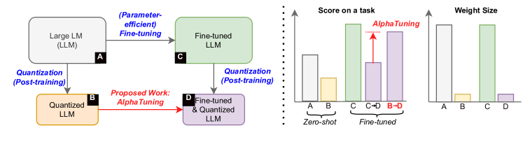
Figure 1: Approaches to satisfy both parameter-efficient adaptation and parameter quantization. Our proposed AlphaTuning technique can achieve 1) competitive performances to fine-tuned LMs (i.e., A$\leadsto$C) with a remarkably reduced parameter size, and 2) significantly better scores than quantized LMs implemented through A$\leadsto$C$\leadsto$D.

Although trainable parameters can be significantly reduced by parameter-efficient adaptation schemes, we notice that the memory footprints for inference are not reduced compared to those of PLMs. To enable efficient deployments of multiple downstream tasks, we incorporate model compression and parameter-efficient adaptation. We argue that previous model compression techniques were not practical solutions in terms of parameter-efficiency for adaptations. For example, Quantization-Aware Training (QAT) Jacob et al. (2018); Esser et al. (2020) can perform full fine-tuning coupled with model compression; however, each task needs dedicated memory storage as much as that of a compressed PLM. Our key observation to achieve a compression-aware parameter-efficient adaptation is that, once a PLM is quantized, only a small amount of quantization-related parameters is needed to be fine-tuned for each target task. As a result, both the overall memory footprints and the number of trainable parameters for adaptation can be substantially reduced.

Figure 1 illustratively compares two different approaches enabling both model compression and parameter-efficient adaptation. Fine-tuned and quantized LMs can be achieved through A$\leadsto$C$\leadsto$D or A$\leadsto$B$\leadsto$D as shown in Figure 1. In the case of A$\leadsto$C$\leadsto$D, we may have a large number of trainable parameters, and/or PTQ may degrade performance on downstream tasks. To address such issues, we investigate A$\leadsto$B$\leadsto$D scheme, called “AlphaTuning” in this work. Specifically, we factorize the parameters of large PLMs into binary values and scaling factors. Then, AlphaTuning conducts the adaptation by training only the scaling factors that occupy a small portion in the quantization format, while freezing the other binary values. Note that, to conduct A$\leadsto$B, we consider post-training quantization (PTQ) Zhao et al. (2019); Hubara et al. (2020); Li et al. (2020a) because the QAT demands significant computational overhead for training from a scratch with the whole dataset.

In this paper, our contributions are as follows:

• To the best of our knowledge, this work is the first successful compression-aware parameter-efficient adaptation method.

• We report that once PLMs are quantized by PTQ, training scaling factors (less than 0.1% of total parameter size) for each task only is enough for successful adaptations.

• Throughout various LMs and tasks, we demonstrate that AlphaTuning can achieve high scores even under 4-bit quantization.

2 Recent Work

Large-Scale Language Models and Quantization

Pre-trained transformer-based language models Devlin et al. (2019); Radford et al. (2019) have shaped the way we design and deploy NLP models. In recent years, the explosion of availability of large-scale (i.e., larger than ten-billion scale) language models Brown et al. (2020); Black et al. (2021); Chowdhery et al. (2022); Zhang et al. (2022a); Hoffmann et al. (2022b) has paved way for a new era in the NLP scene, where few-shot learning and the parameter-efficient adaptation for downstream tasks will be more important He et al. (2021). The quantization (that we discuss in detail in the next section) is an effective approach to fundamentally overcome the space and time complexities of the large-scale language models Zafrir et al. (2019); Bondarenko et al. (2021), but existing methods are only applicable to limited domains and task adaptability under the quantized state.

Parameter-Efficient Adaptation of LMs

Adapting language models efficiently for a task and domain-specific data has been at the center of the community’s interests since the emergence of large-scale language models. One promising approach is in-context learning (ICL) Brown et al. (2020), in which the language model learns and predicts from the given prompt patterns. As the technique elicits reasonable few-shot performances from the large-scale language models without parameter-tuning, a plethora of works Zhao et al. (2021); Lu et al. (2022); Reynolds and McDonell (2021); Min et al. (2022) have investigated the underlying mechanism and proposed various methods to further exploit this approach. Another class of techniques is to adopt external or partially internal parameters such as continuous prompt embeddings to enable parameter-efficient LM adaptation, which is based on the intuition that specific prompt prefixes may better elicit certain LM behaviors. Earlier works explored the discrete prompt token space Shin et al. (2020), but later work showed that optimizing on the continuous word embedding space yielded better results Liu et al. (2021b); Li and Liang (2021); Gu et al. (2022), even performing on par with full fine-tuning Lester et al. (2021); Vu et al. (2022). Another similar line of works explored introducing new parameters within the Transformer blocks or partially training existing parameters Houlsby et al. (2019); Zhang et al. (2020); Karimi Mahabadi et al. (2021); Hu et al. (2022). Finally, some works have suggested unifying all existing approaches related to parameter-efficient fine-tuning He et al. (2021); Zhang et al. (2022b).

Layer	${\bm{W}}$ Shape	${\bm{W}}$ Size	$g$	$\alpha\in\mathbb{R}$	$B\in\{$-1,+1$\}$	Quantized ${\bm{W}}$ Size (MB)
	($h_{out}$, $h_{in}$)	(FP32)		Shape	Shape	$q=1$	$q=2$	$q=3$
ATT_qkv	($3h,h$)	12.58 MB	$h$	($q,3h$)	($q,3h,h$)	0.41	0.81	1.22
ATT_output	($h,h$)	4.19 MB	$h$	($q,h$)	($q,h,h$)	0.14	0.27	0.41
FFN_h_4h	($4h,h$)	16.78 MB	$h$	($q,4h$)	($q,4h,h$)	0.54	1.08	1.62
FFN_4h_h	($h,4h$)	16.78 MB	4$h$	($q,h$)	($q,h,4h$)	0.52	1.06	1.56
			$h$	($q,4h$)	($q,4h,h$)	0.54	1.08	1.62
			0.5$h$	($q,8h$)	($q,8h,h$)	0.56	1.11	1.67

Table 1: BCQ scheme for $q$-bit quantization applied to linear layers of the Transformers and examples of BCQ formats for GPT-2 medium model (hidden size $h$ is 1024). Row-wise quantization is performed when $g=h_{in}$. Lower $g$ results in slightly increased weight size after quantization.

3 Quantization for AlphaTuning

Enterprise-scale LMs, such as 175B GPT-3, face challenges in the prohibitive cost of massive deployment mainly resulting from their huge parameter size. To facilitate cost-effective LMs by alleviating memory requirements without noticeable performance degradation, we can consider compression techniques, such as quantization (Jacob et al., 2018), pruning (Frankle et al., 2020a), and low-rank approximation (N. Sainath et al., 2013). Memory reduction by model compression is also useful to reduce latency because memory-bound operations dominate the overall performance of LMs with a small batch size (Park et al., 2022). In addition, model compression can save the number of GPUs for inference because GPUs present highly limited memory capacity (Shoeybi et al., 2019; Narayanan et al., 2021). In this work, we choose quantization as a practical compression technique because of its high compression ratio, simple representation format, and the capability to accelerate memory-bound workloads (Chung et al., 2020).

Let us discuss our quantization strategy for LMs (see more details in Appendix C). We choose non-uniform quantization since uniform quantization demands aggressive activation quantization (to exploit integer arithmetic units) which is challenged by highly non-linear operations (such as softmax and layer normalization) of the Transformers Bondarenko et al. (2021). Even though uniform quantization can mitigate performance degradation by frequent activation quantization/dequantization procedures Bhandare et al. (2019) or additional high-precision units Kim et al. (2021b), such techniques are slow and/or expensive. Among various non-uniform quantization formats, we choose binary-coding-quantization (BCQ) Guo et al. (2017); Xu et al. (2018) which is extended from binary neural networks Rastegari et al. (2016) because of high compression ratio Chung et al. (2020) and efficient computations Xu et al. (2018); Jeon et al. (2020).

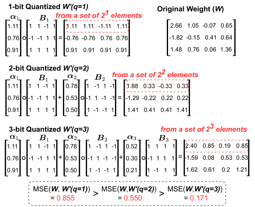
Figure 2: BCQ examples with $g=4$ and different $q$ values. As $q$ increases, the MSE between the original weight and the quantized weight decreases.

BCQ Format

Given a full-precision weight vector ${\bm{w}}\in\mathbb{R}^{g}$, BCQ format approximates ${\bm{w}}$ to be ${\bm{w}}\approx\sum_{i=1}^{q}\alpha_{i}{\bm{b}}_{i}$ where $q$ is the number of quantization bits, $\alpha\in\mathbb{R}$ is a scaling factor to be shared by $g$ weights, and ${\bm{b}}\in\{-1,+1\}^{g}$ is a binary vector. Note that $g$ represents a group size or the number of weights sharing a common scaling factor. Thus, $g$ is a hyper-parameter for quantization. When $q$=1, $\alpha$ and ${\bm{b}}$ can be analytically determined to minimize the mean squared error (MSE). If $q>1$, however, $\alpha$ and ${\bm{b}}$ need to be obtained by heuristic methods such as greedy approximation Guo et al. (2017) and iterative fine-tuning method Xu et al. (2018).

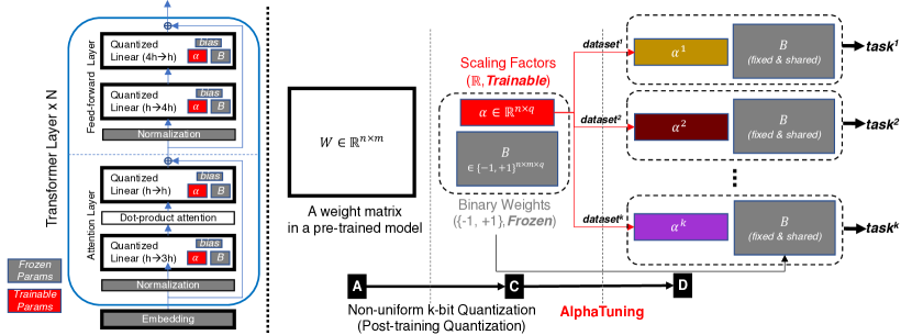
Figure 3: (Left): Quantized Transformer structure in which parameters are categorized into frozen ones and trainable ones. (Right): Overview of AlphaTuning process that trains scaling factors only for adaptation.

For a weight matrix ${\bm{W}}\in\mathbb{R}^{h_{out}{\times}h_{in}}$, row-wise quantization (i.e., $g=h_{in}$) is a popular choice Jeon et al. (2020); Xu et al. (2018) and can be expressed as follows:

$${\bm{W}}\approx\sum_{i=1}^{q}\text{diag}(\bm{\alpha}_{i})\cdot{\bm{B}}_{i},$$ (1)

where $\bm{\alpha}_{i}\in\mathbb{R}^{h_{out}}$, ${\bm{B}}_{i}\in{\{-1,+1\}}^{h_{out}{\times}h_{in}}$, and $\text{diag}(\cdot)$ denotes the function of a vector that outputs a zero-matrix except for the vector elements in its diagonal. A linear operation of ${\bm{Y}}={\bm{X}}\cdot({\bm{W}})^{\top}$, then can be approximated as follows:

$${\bm{Y}} ={\bm{X}}\cdot{\bm{W}}^{\top}$$ (2)

$$\approx{\bm{X}}\cdot\left(\sum_{i=1}^{q}\text{diag}\left(\bm{\alpha}_{i}\right)\cdot{\bm{B}}_{i}\right)^{\top}$$

$$=\sum_{i=1}^{q}\Big{(}({\bm{X}}\cdot{\bm{B}}_{i}^{\top})\cdot\text{diag}\left(\bm{\alpha}_{i}\right)\Big{)},$$

where ${\bm{X}}\in\mathbb{R}^{n_{b}{\times}h_{in}}$, and ${\bm{Y}}\in\mathbb{R}^{n_{b}{\times}h_{out}}$. Note that even though ${\bm{X}}$ is not quantized above, most complicated floating-point operations are removed due to binary values in ${\bm{B}}$. Since the computational advantages of BCQ have been introduced in the literature (Hubara et al., 2016; Jeon et al., 2020), we do not quantize activations in this work to improve quantization quality.

Figure 2 describes the row-wise BCQ examples based on greedy approximation Guo et al. (2017) when $q$ varies. Note that increasing $q$ and/or decreasing $g$ can reduce the MSE after quantization at the cost of a lower compression ratio.

Transformer Quantization

Table 1 presents our BCQ scheme applied to linear layers of the Transformers while BCQ formats are illustrated for the medium-sized GPT-2 model (that has a hidden size ($h$) of 1024). Note that if $g$ is large enough such that each scaling factor is shared by many weights, the amount of scaling factors is ignorable compared to that of ${\bm{B}}$. In Table 1, hence, 1-bit quantization attains almost 32$\times$ compression ratio compared to FP32 format while lower $g$ slightly increases storage overhead induced by additional scaling factors.

4 AlphaTuning: Efficient Fine-Tuning of Quantized Models

Model	Method	$q$	Trainable	Model Size		Valid Loss	BLEU (95% Confidence Interval)
			Params	CKPT	Total		Unseen	Seen	All
GPT-2 M	FT (Fine-Tuning)	-	354.9M	1420MB	1420MB	0.79	$32.7_{\pm.6}$	$62.0_{\pm.4}$	$48.4_{\pm.3}$
	$\Rightarrow$ PTQ(WFT)1	3	-	327MB	327MB	2.03	$25.0_{\pm 2.5}$	$58.7_{\pm 1.0}$	$43.2_{\pm 3.3}$
	LoRA	-	0.35M	1.4MB	1420MB	0.81	$45.5_{\pm.4}$	$64.3_{\pm.2}$	$55.8_{\pm.3}$
	$\Rightarrow$ PTQ(W)+WLoRA2	3	-	1.4MB	328MB	2.98	$15.8_{\pm 3.0}$	$15.8_{\pm 3.4}$	$15.8_{\pm 3.2}$
	$\Rightarrow$ PTQ(W+WLoRA)3	3	-	327MB	327MB	3.36	$12.6_{\pm 4.1}$	$16.6_{\pm 6.7}$	$13.6_{\pm 7.5}$
	AlphaTuning	3	0.22M	0.9MB	327MB	0.81	$40.9_{\pm.5}$	$63.2_{\pm.5}$	$53.1_{\pm.4}$
	AlphaTuning	2	0.22M	0.9MB	289MB	0.84	$37.3_{\pm.5}$	$62.6_{\pm.5}$	$51.3_{\pm.5}$
GPT-2 L	FT (Fine-Tuning)	-	774.0M	3096MB	3096MB	0.81	$23.8_{\pm.3}$	$60.8_{\pm.1}$	$43.0_{\pm.3}$
	$\Rightarrow$ PTQ(WFT)	3	-	535MB	535MB	1.90	$23.2_{\pm.8}$	$62.7_{\pm.2}$	$43.7_{\pm.7}$
	LoRA	-	0.77M	3.1MB	3096MB	0.79	$48.4_{\pm.3}$	$64.0_{\pm.3}$	$57.0_{\pm.1}$
	$\Rightarrow$ PTQ(W)+WLoRA	3	-	3.1MB	538MB	1.97	$20.1_{\pm 5.2}$	$27.8_{\pm 4.1}$	$24.1_{\pm 4.5}$
	$\Rightarrow$ PTQ(W+WLoRA)	3	-	535MB	535MB	1.97	$14.0_{\pm 7.2}$	$26.6_{\pm 11.5}$	$25.8_{\pm 13.0}$
	AlphaTuning	3	0.42M	1.7MB	535MB	0.84	$47.0_{\pm.6}$	$62.2_{\pm.2}$	$55.3_{\pm.3}$
	AlphaTuning	2	0.42M	1.7MB	445MB	0.82	$42.7_{\pm.4}$	$62.9_{\pm.4}$	$53.8_{\pm.1}$
	AlphaTuning	1	0.42M	1.7MB	355MB	0.87	$28.1_{\pm.3}$	$62.3_{\pm.7}$	$47.1_{\pm.4}$

• Fully fine-tuned LMs are quantized by PTQ using the Alternating method.

• For inference, quantized PLMs (by the Alternating method) are dequantized to be merged with trainable parameters for LoRA. This method is parameter-efficient but we have low scores and dequantization overhead.

• After LoRA, frozen weights and trainable weights are merged and then quantized (by the Alternating method). Since PTQ is applied to the merged weights, each task needs to store the entire (quantized) model.

Table 2: Validation loss and test scores on WebNLG with various adaptation methods using GPT-2 models (see Table 10 in Appendix for hyper-parameter selections and Table 8 in Appendix additional scores). For full fine-tuning and LoRA, we explored learning rates and weight decay factors while the other hyper-parameters are from Hu et al. (2022). $g$ is selected to be $h_{in}$ in each layer for row-wise quantization.

4.1 AlphaTuning Principles

The key idea of AlphaTuning is identifying parameters presenting greater expressive power to minimize the number of trainable parameters after PTQ. Note that training affine parameters (that transform the activations through operations such as scaling, shifting, and rotating) reportedly achieves reasonably high accuracy even when all the other parameters are fixed to be random Frankle et al. (2020b). Interestingly, scaling factors obtained by the BCQ format can be regarded as affine parameters as shown in Eq. 2. Based on such observation, Figure 3 presents the overview of AlphaTuning. First, we quantize the weights of linear layers of the Transformers that dominate the overall memory footprint Park et al. (2022). Then, the BCQ format factorizes the quantized weights into scaling factors and binary values. Finally, the scaling factors are trained for a given target task and all the other parameters (e.g., biases, binary values ${\bm{B}}$, and those of the normalization layer and embedding layer) are frozen regardless of downstream tasks.

Training Algorithm

For a linear layer quantized by Eq. 1, the forward propagation can be performed without dequantizing ${\bm{W}}$ and be described as Eq. 2. Similarly, the backward propagation can also be computed in the quantized format and the gradients of ${\bm{W}}$ and $\bm{\alpha}$ with respect to ${\bm{Y}}$ (to conduct the chain rule) are obtained as follows:

$$\partial{{\bm{X}}}=\partial{\bm{Y}}\cdot\Big{(}\sum_{i=1}^{q}\text{diag}(\bm{\alpha}_{i})\cdot{\bm{B}}_{i}\Big{)}$$ (3)

$$\partial{\bm{\alpha}}_{i}=\frac{(\partial{\bm{Y}})^{\top}{\bm{X}}{\bm{B}}_{i}^{\top}\cdot\mathds{1}^{\top}}{g_{L}}\,(1\leq i\leq q),$$ (4)

where $\mathds{1}$ is an $h_{out}$-long all-ones vector and $g_{L}$ is the group size of the layer $L$. Note that dividing by $g_{L}$ is empirically introduced in Eq. 4 to prevent excessively large $\alpha$ updates and to enhance the stability of training. Even if $g_{L}\neq h_{in}$ (i.e., other than row-wise quantization), we still can utilize the same equations by using tiling-based approaches Jeon et al. (2020).

4.2 AlphaTuning for GPT-2

We apply AlphaTuning to GPT-2 medium and large on WebNLG Gardent et al. (2017) to explore a hyper-parameter space and investigate the effects of AlphaTuning as shown in Table 2. Note that in this paper, we assume that parameters (including $\alpha$) are represented as 32-bit floating-point numbers (i.e., FP32 format) unless indicated to be compressed by $q$-bit quantization.

Hyper-Parameter	Base	Trial	Loss	Unseen	Seen	All
Trainable Params	0.22M ($\bm{\alpha}_{1}$)	0.66M ($\bm{\alpha}_{1}$,$\bm{\alpha}_{2}$,$\bm{\alpha}_{3}$)	0.76	$40.6\pm.4$	$63.2\pm.2$	$53.1\pm.1$
Dropout Rate	0.0	0.1	0.81	$42.4\pm.3$	$61.2\pm.4$	$52.7\pm.2$
PTQ Method	Greedy	Alternating	0.80	$41.0\pm.6$	$63.0\pm.3$	$53.0\pm.3$
LR Warm-up	0 steps	500 steps	0.81	$41.0\pm.2$	$63.3\pm.1$	$53.3\pm.1$
Epochs	5 epochs	3 epochs	0.82	$42.2\pm.6$	$62.9\pm.4$	$53.6\pm.4$
Epochs	5 epochs	10 epochs	0.82	$38.5\pm.7$	$62.7\pm.5$	$51.9\pm.4$
Base Hyper-Parameter Selection (Table 2)			0.81	$40.9\pm.5$	$63.2\pm.5$	$53.1\pm.4$

Table 3: Experimental results on WebNLG to investigate the impact of hyper-parameter selection for AlphaTuning on GPT-2 medium quantized by PTQ using 3-bit quantization (i.e., $q=3$). Test BLEU scores are averaged over 5 trials with the same learning rates and weight dacay fectors in Table 2.

Adaptation Details

PTQ for AlphaTuning is performed on the pre-trained GPT-2 by the Greedy method Guo et al. (2017). Then, for $q$-bit quantization, we train only $\bm{\alpha}_{1}$ among $\bm{\alpha}_{1}\cdots\bm{\alpha}_{q}$ to maximize parameter-efficiency of adaptation because training all $\bm{\alpha}$ values provides only marginal gains as shown in Table 3. Training $\bm{\alpha}_{1}$ is performed by a linear decay learning rate schedule without dropout. For each hyper-parameter selection, test scores are measured at the 5^th epoch and averaged over 5 trials (along with 5 random seeds which are fixed for the experiments in Table 3 justifying our hyper-parameter selections). For all adaptation methods considered in Table 2, learning rates and weight decay factors are explored to produce the best at ‘all’ category (see Table 11 for exploration results on AlphaTuning).

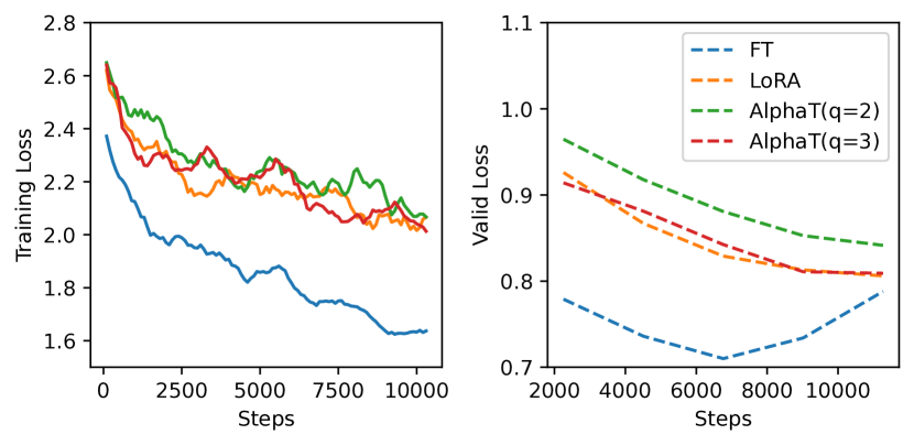
(a) GPT-2 Medium

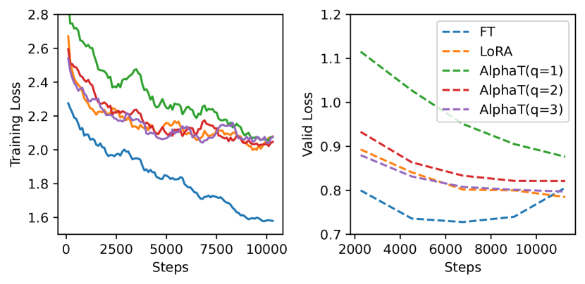
(b) GPT-2 Large

Figure 4: Training/validation loss on WebNLG by full fine-tuning, LoRA, and AlphaTuning ($q=2$ or 3).

Comparison with Fine-Tuning and LoRA

We compare AlphaTuning with full fine-tuning and LoRA reproduced by using hyper-parameters (except learning rates and weight decay factors) in Hu et al. (2022) for WebNLG. As shown in Table 2, AlphaTuning provides BLUE scores which are comparable to that of LoRA and better than that of full fine-tuning, while both total memory footprint and checkpoint (CKPT) memory sizes are significantly reduced. The different scores can be partly explained by Figure 4 showing that the training process by AlphaTuning or LoRA converges well while the full fine-tuning causes overfitting. Interestingly, even though we train only $\bm{\alpha}_{1}$ (and hence, $\bm{\alpha}_{2}$ and $\bm{\alpha}_{3}$ are fixed for all tasks), increasing $q$ improves the validation loss and the test BLEU scores. Note that as $q$ increases, ‘Unseen’ scores are enhanced rapidly while ‘Seen’ scores are not affected noticeably. Overall, AlphaTuning with the 3-bit (i.e., $q=3$) quantization can be a successful parameter-efficient adaptation with a high compression ratio.

$g$	Params	Loss	Unseen	Seen	All
64	4.72M	0.78	$42.7_{\pm.3}$	$64.2_{\pm.2}$	$54.5_{\pm.2}$
256	1.18M	0.77	$41.7_{\pm.4}$	$63.9_{\pm.3}$	$54.0_{\pm.2}$
512	0.59M	0.77	$41.2_{\pm.7}$	$63.7_{\pm.1}$	$53.7_{\pm.3}$
1K	0.30M	0.79	$40.9_{\pm.6}$	$63.6_{\pm.5}$	$53.4_{\pm.3}$
$h_{in}$	0.22M	0.81	$40.9_{\pm.5}$	$63.2_{\pm.5}$	$53.1_{\pm.4}$
2K	0.15M	0.84	$40.9_{\pm.4}$	$62.5_{\pm.7}$	$52.8_{\pm.4}$

Table 4: Impact of $g$ (group size) when AlphaTuning ($q$=3) is applied to GPT-2 medium on WebNLG. When $g=h_{in}$, row-wise quantization is indicated.

Model	Method	$q$	Trainable Params	Valid Loss	BLEU	METEOR	TER
GPT-2 Medium	Fine-Tuning	-	354.92M	-	$46.0_{\pm 0.1}$	$0.39$	$0.46$
	LoRA	-	0.35M	-	$47.1_{\pm 0.2}$	$0.39$	$0.46$
	AlphaTuning	3	0.22M	1.13	$46.6_{\pm 0.2}$	$0.38$	$0.48$
	AlphaTuning	2	0.22M	1.17	$45.7_{\pm 0.2}$	$0.38$	$0.49$
GPT-2 Large	FineTuning	-	774.03M	-	$46.5_{\pm 0.1}$	$0.39$	$0.45$
	LoRA	-	0.77M	-	$47.5_{\pm 0.2}$	$0.38$	$0.45$
	AlphaTuning	3	0.42M	1.08	$47.8_{\pm 0.2}$	$0.39$	$0.47$
	AlphaTuning	2	0.42M	1.10	$47.2_{\pm 0.2}$	$0.38$	$0.47$

Table 5: Test scores on DART with various adaptation methods using GPT-2 models (see Table 10 in Appendix for hyper-parameter selections). The checkpoint and weight sizes can be found in Table 2. The results of full fine-tuning and LoRA are quoted from Hu et al. (2022). $g$ is selected to be $h_{in}$ in each layer for row-wise quantization. For all METEOR and TER scores in the table, the variances are less than 0.01.

Comparison with A$\leadsto$C$\leadsto$D in Figure 1

As potentially alternative methods of AlphaTuning, we investigate the following three cases: 1) applying PTQ to a fully fine-tuned model (i.e., PTQ(W_FT)), 2) applying PTQ to a PLM and then LoRA parameters are augmented (i.e., PTQ(W)+W_LoRA), and 3) a PLM and LoRA parameters are merged and then quantized (i.e., PTQ(W+W_LoRA)). Such three cases induce various checkpoint sizes, total model sizes, and the number of trainable parameters as shown in Table 2. Note that the scores of PTQ(W)+W_LoRA and PTQ(W+W_LoRA) are degraded significantly. In other words, model compression techniques and parameter-efficient adaptation methods may have conflicting properties when combined in a straightforward manner. Even though PTQ(W_FT) shows better scores than the other two cases, the number of trainable parameters remains to be the same as that of full fine-tuning and checkpoint size for a task is considerably larger than that of LoRA and AlphaTuning. By contrast, AlphaTuning offers acceptable BLEU scores even with a smaller number of trainable parameters and a smaller checkpoint size than those three cases.

Hyper-Parameter Selection

A few hyper-parameters (such as dropout rate and the number of epochs) are related to the trade-off between ‘Unseen’ score and ‘Seen’ score as described in Table 3. In the case of PTQ method, even when the Alternating method Xu et al. (2018) is employed with many iterations to further reduce MSE, the scores become similar to that of the Greedy method after adaptation. As such, we choose the Greedy method for all tasks in this paper. The learning rate warm-up seems to present random effects depending on PLM, downstream task, and $q$ selection. The group size $g$ provides the clear trade-off between the trainable parameter size and test scores as shown in Table 4. Unless stated otherwise, we choose $g=h_{in}$ (i.e., row-wise quantization) in this paper.

5 Experimental Results

Model	Method	$q$	Trainable	Valid	Test Scores
			Params	Loss	BLEU	NIST	METEOR	ROUGE_L	CIDEr
GPT-2 M	Fine-Tuning	-	354.92M	1.28	$67.5_{\pm.2}$	$8.60_{\pm.02}$	$46.4_{\pm.2}$	$70.8_{\pm.2}$	$2.40_{\pm.01}$
	$\Rightarrow$ PTQ(WFT)	3	-	1.19	$67.5_{\pm.5}$	$8.58_{\pm.04}$	$46.3_{\pm.5}$	$70.3_{\pm.1}$	$2.39_{\pm.01}$
	LoRA	-	0.35M	1.16	$70.2_{\pm.2}$	$8.80_{\pm.04}$	$46.8_{\pm.1}$	$71.7_{\pm.4}$	$2.53_{\pm.01}$
	$\Rightarrow$ PTQ(W)+WLoRA	3	-	4.10	$11.1_{\pm 5.3}$	$2.35_{\pm 1.04}$	$12.4_{\pm 4.2}$	$29.9_{\pm 7.8}$	$0.35_{\pm.18}$
	$\Rightarrow$ PTQ(W+WLoRA)	3	-	4.38	$7.5_{\pm 3.2}$	$1.31_{\pm.21}$	$11.4_{\pm.8}$	$29.8_{\pm 3.0}$	$0.29_{\pm.04}$
	AlphaTuning	3	0.22M	1.18	$69.9_{\pm.3}$	$8.79_{\pm.05}$	$46.7_{\pm.2}$	$71.7_{\pm.3}$	$2.51_{\pm.01}$
	AlphaTuning	2	0.22M	1.20	$70.0_{\pm.4}$	$8.80_{\pm.05}$	$46.7_{\pm.1}$	$71.6_{\pm.5}$	$2.51_{\pm.01}$
GPT-2 L	Fine-Tuning	-	774.03M	1.31	$67.2_{\pm.3}$	$8.61_{\pm.05}$	$46.3_{\pm.1}$	$70.5_{\pm.3}$	$2.37_{\pm.01}$
	$\Rightarrow$ PTQ(WFT)	3	-	0.98	$66.5_{\pm 1.0}$	$8.45_{\pm.10}$	$45.7_{\pm.3}$	$70.3_{\pm.5}$	$2.37_{\pm.03}$
	LoRA	-	0.77M	1.13	$69.8_{\pm.2}$	$8.80_{\pm.03}$	$46.6_{\pm.1}$	$71.7_{\pm.1}$	$2.51_{\pm.01}$
	$\Rightarrow$ PTQ(W)+WLoRA	3	-	1.87	$50.9_{\pm 3.4}$	$6.63_{\pm.32}$	$38.7_{\pm 1.9}$	$60.6_{\pm 1.9}$	$1.30_{\pm.19}$
	$\Rightarrow$ PTQ(W+WLoRA)	3	-	1.76	$53.7_{\pm 3.1}$	$7.12_{\pm.37}$	$40.0_{\pm 1.5}$	$61.7_{\pm 1.1}$	$1.5_{\pm.11}$
	AlphaTuning	2	0.42M	1.14	$69.7_{\pm.6}$	$8.78_{\pm.08}$	$46.6_{\pm.2}$	$71.5_{\pm.3}$	$2.51_{\pm.03}$
	AlphaTuning	1	0.42M	1.18	$69.7_{\pm.3}$	$8.79_{\pm.03}$	$46.6_{\pm.1}$	$71.6_{\pm.2}$	$2.51_{\pm.02}$

Table 6: Validation loss and test scores on E2E with various adaptation methods using GPT-2 models (see Table 10 in Appendix for hyper-parameter selections). The number of trainable parameters, checkpoint sizes, and weight sizes are the same as in Table 2. For full fine-tuning and LoRA, we explored learning rates and weight decay factors while the other hyper-parameters are quoted from Hu et al. (2022). $g$ is selected to be $h_{in}$ in each layer for row-wise quantization.

Method	$q$	$g$	MNLI			SAMSum
			Trainable	Wight	Accuracy	Trainable	Weight	R1 / R2 / RL
			Params	Size	(%)	Params	Size
Fine-Tuning	-	-	1315.76M	5.26GB	$83.6$	1315.75M	5.26GB	$49.4$ / $25.3$ / $40.5$
$\Rightarrow$ PTQ(WFT)	4	$h$	-	1.04GB	$76.7$	-	1.04GB	$13.0$ / $5.5$ / $11.4$
AlphaTuning	4	$0.5h$	1.19M	1.05GB	$82.7$	1.18M	1.05GB	$47.5$ / $24.1$ / $38.9$
AlphaTuning	4	$h$	0.60M	1.04GB	$82.3$	0.59M	1.04GB	$47.3$ / $23.2$ / $38.4$
AlphaTuning	3	$0.5h$	1.19M	0.90GB	$82.4$	1.18M	0.90GB	$47.4$ / $24.2$ / $39.0$
AlphaTuning	3	$h$	0.60M	0.89GB	$82.4$	0.59M	0.89GB	$46.5$ / $22.8$ / $37.8$

Table 7: Validation scores on MNLI dataset and test scores on SAMSum dataset with full fine-tuning and AlphaTuning using OPT 1.3B model for which hidden size $h$ is 2048 (see Appendix B for experimental details).

To extensively demonstrate the influence of AlphaTuning, we apply detailed adaptation techniques and hyper-parameter selections that we explored by using GPT-2 models on WebNLG (in the previous section) to additional downstream tasks and OPT models Zhang et al. (2022a).

5.1 GPT-2 Models on DART and E2E

Adaptations using full fine-tuning, LoRA, and AlphaTuning methods based on pre-trained GPT-2 medium/large are performed on DART Nan et al. (2021) and E2E Novikova et al. (2017). As for DART dataset, we observe (in Table 5) AlphaTuning even with an extreme quantization (e.g., $q=2$) can maintain test scores to be similar to those of LoRA and full fine-tuning, both of which do not consider model compression. In the case of E2E dataset, we find that 1) full fine-tuning suffers from degraded test scores, 2) even AlphaTuning with $q=1$ is a reasonable choice for GPT-2 large, and 3) quantizing a model (after being adapted by LoRA) destroys test scores. All in all, when combined with pre-trained GPT-2 medium/large on various tasks, AlphaTuning turns out to be effective for both a high compression ratio and a massive reduction in the number of trainable parameters.

5.2 OPT Models on MNLI and SAMSum

We utilize a pre-trained OPT 1.3B model to be adapted through full fine-tuning or AlphaTuning on GLUE-MNLI Williams et al. (2018) and SAMSum Gliwa et al. (2019). For text classification on MNLI, an LM head layer is added on top of GPT-2 with randomly initialized weights Radford et al. (2019). As evidenced by Table 7, we find the following results: 1) PTQ(W_FT) sometimes results in severely impaired scores (e.g., on SAMSum dataset) even when computations for PTQ are associated with a lot of iterations; 2) AlphaTuning outperforms PTQ(W_FT) scheme (for the whole tasks in this paper), and 3) decreasing $g$ of AlphaTuning can improve scores.

6 Discussion

Memory during Adaptation

As a compression-aware parameter-efficient adaptation technique, AlphaTuning reduces not only inference memory footprints (by quantization) and also training memory footprints during adaptation. Specifically, optimizer states to be stored in GPU memory are derived only by scaling factors that occupy less than 0.1% of total weight size if $g$ is large enough. Such reduced GPU memory requirements during training correspond to increased batch size or a reduced minimum number of GPUs performing adaptation.

Embedding Layers

In this work, we considered linear layers of the Transformers to be quantized by BCQ while embedding layers remain to be of full precision. The rationale behind this choice is that as the model scales with a larger hidden size ($h$), the relative size of embedding layers becomes smaller. To be more specific, the space complexities of linear layers and embedding layers follow $\mathcal{O}(h^{2})$ and $\mathcal{O}(h)$, respectively. As such, for large-scale LMs, we expect quantizing embedding layers to produce only marginal improvements on a compression ratio while test scores might be degraded.

Inference Speed

As described in Eq. 2, BCQ format enables unique computations for matrix multiplications even when activations are not quantized. Recent works Jeon et al. (2020); Park et al. (2022) show that matrix multiplications based on BCQ format can be expedited by the following operations: 1) compute all possible computations (combining partial activations and ${\bm{B}}$) in advance and store them in look-up tables (LUTs) and 2) let LUT retrievals (using ${\bm{B}}$ values as indices) replace floating-point additions in Eq. 2. The major reasons for fast computations are due to byte-level accesses of LUTs and increased LUT reuse by increased $h$ Jeon et al. (2020); Park et al. (2022). Such LUT-based matrix multiplications can lead to latency improvement as much as a memory reduction ratio.

7 Conclusion

In this paper, we proposed AlphaTuning as the first successful compression-aware parameter-efficient adaptation method for large-scale LMs. Through a few representative generative LMs (such as GPT-2), we demonstrated that once linear layers are quantized by BCQ format, training only scaling factors can obtain reasonably high scores. We also empirically proved that quantizing an already adapted LMs would degrade scores significantly. Incorporating various model compression techniques and parameter-efficient adaptation methods would be an interesting research topic in the future.

Limitations

We believe that the major contributions in this paper would become more convincing as the size of the PLM increases, whereas the models used for experiments in this paper (i.e., GPT-2 and 1.3B OPT) may not be large enough compared to the large-scale LMs recently announced (e.g., OPT 175B). Considering a few reports that larger models tend to be compressed by a higher compression ratio along with less performance degradation Li et al. (2020b), we expect AlphaTuning to be effective as well even for larger models, to say, of more than 10 billion of parameters.

The performance of AlphaTuning on 1.3B OPT becomes better than that of PTQ(W_FT), but inferior to that of the full fine-tuning. We suspect such results might result from insufficient search of an appropriate training recipe for AlphaTuning. Correspondingly, exploring learning hyper-parameters of AlphaTuning using larger LMs and more datasets would be required to yield general claims on the characteristics of AlphaTuning.

Ethics Statement

Large language models (LMs) such as GPT-3 (Brown et al., 2020), Gopher (Rae et al., 2021), PaLM (Chowdhery et al., 2022), and HyperCLOVA (Kim et al., 2021a) have shown surprising capabilities and performances for natural language understanding and generation, in particular, an in-context zero or few-shot manner. They can provide innovative applications such as code generation (Chen et al., 2021) and text-to-image generation Ramesh et al. (2021) via fine-tuning with additional data dedicated to each task. Despite their astonishing advantages, it is well known that large LMs have severe and challenging limitations for deployment to user applications, such as biased and toxic expression, hallucination, too heavy energy consumption, and carbon emission (Weidinger et al., 2021). Our work aims to address the energy issue of large LMs in terms of inference and deployment. We expect that our method can alleviate energy consumption by reducing practical memory footprints and latency when the large LMs are deployed to various user applications. We might need to address the other ethical issues through further research for safer and better contributions of the large LMs.

Size	Method	$q$	BLEU			METEOR			TER
			U	S	A	U	S	A	U	S	A
GPT M	FT(Fine-Tuning)	-	$32.7_{\pm.6}$	$62.0_{\pm.4}$	$48.4_{\pm.3}$	$.32$	$.45$	$.39$	$.63$	$.33$	$.47$
	$\Rightarrow$ PTQ(WFT)	3	$25.0_{\pm 2.5}$	$58.7_{\pm 1.0}$	$43.2_{\pm 3.3}$	$.28$	$.43$	$.36$	$.87$	$.37$	$.60$
	LoRA	-	$45.5_{\pm.4}$	$64.3_{\pm.2}$	$55.8_{\pm.3}$	$.38$	$.45$	$.42$	$.47$	$.32$	$.39$
	$\Rightarrow$ PTQ(W)+WLoRA	3	$15.8_{\pm 3.0}$	$15.8_{\pm 3.4}$	$15.8_{\pm 3.2}$	$.20$	$.21$	$.21$	$1.03$	$1.20$	$1.12$
	$\Rightarrow$ PTQ(W+WLoRA)	3	$12.6_{\pm 4.1}$	$16.6_{\pm 6.7}$	$13.6_{\pm 7.5}$	$.17$	$.18$	$.18$	$.72$	$.70$	$.68$
	AlphaTuning	3	$40.9_{\pm.5}$	$63.2_{\pm.5}$	$53.1_{\pm.4}$	$.35$	$.44$	$.40$	$.51$	$.33$	$.42$
	AlphaTuning	2	$37.3_{\pm.5}$	$62.6_{\pm.5}$	$51.3_{\pm.5}$	$.33$	$.44$	$.39$	$.55$	$.33$	$.43$
GPT L	FT(Fine-Tuning)	-	$23.8_{\pm.3}$	$60.8_{\pm.1}$	$43.0_{\pm.3}$	$.27$	$.45$	$.36$	$.77$	$.34$	$.54$
	$\Rightarrow$ PTQ(WFT)	3	$23.2_{\pm.8}$	$62.7_{\pm.2}$	$43.7_{\pm.7}$	$.27$	$.45$	$.36$	$.77$	$.33$	$.54$
	LoRA	-	$48.4_{\pm.3}$	$64.0_{\pm.3}$	$57.0_{\pm.1}$	$.39$	$.45$	$.42$	$.45$	$.32$	$.38$
	$\Rightarrow$ PTQ(W)+WLoRA	3	$20.1_{\pm 5.2}$	$27.8_{\pm 4.1}$	$24.1_{\pm 4.5}$	$.21$	$.25$	$.23$	$.99$	$.84$	$.91$
	$\Rightarrow$ PTQ(W+WLoRA)	3	$14.0_{\pm 7.2}$	$26.6_{\pm 11.5}$	$25.8_{\pm 13.0}$	$.16$	$.23$	$.23$	$1.24$	$.76$	$.79$
	AlphaTuning	3	$47.0_{\pm.6}$	$62.2_{\pm.2}$	$55.3_{\pm.3}$	$.38$	$.43$	$.41$	$.46$	$.33$	$.39$
	AlphaTuning	2	$42.7_{\pm.4}$	$62.9_{\pm.4}$	$53.8_{\pm.1}$	$.36$	$.44$	$.40$	$.49$	$.33$	$.41$
	AlphaTuning	1	$28.1_{\pm.3}$	$62.3_{\pm.7}$	$47.1_{\pm.4}$	$.29$	$.44$	$.36$	$.66$	$.33$	$.49$

Table 8: Additional scores on WebNLG using GPT-2 (Extended results of Table 2) including METEOR and TER scores (U: Unseen, S:Seen, A: All). Lower TER score indicates better generation capability while other scores are to be higher for better capability. For METEOR and TAR scores, the variances of all the cases are less than 0.01.

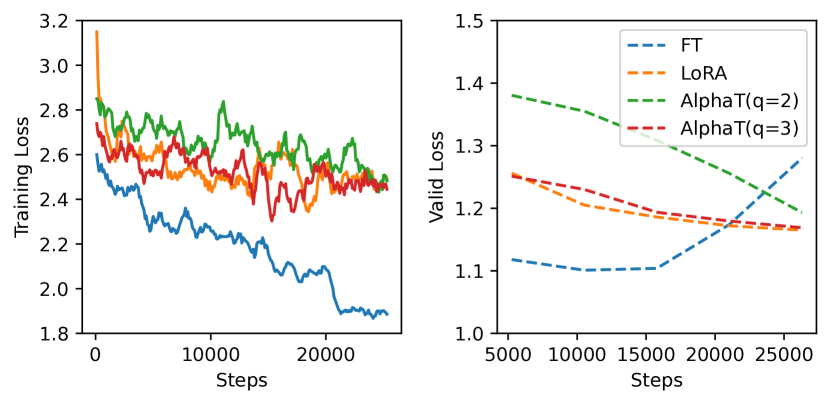
(a) GPT-2 Medium

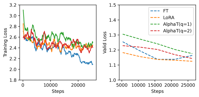
(b) GPT-2 Large

Figure 5: Training/validation loss on E2E by full fine-tuning, LoRA, and AlphaTuning ($q$=1, 2, or 3)

Appendix A Experimental Details on GPT-2 Models

For all the adaptation experiments, we utilize the pre-trained GPT-2 Medium/Large models provided by HuggingFace Wolf et al. (2020). GPT-2 Medium consists of 24 Transformer layers with a hidden size ($h$) of 1024 and GPT-2 Large is composed of 36 Transformer layers with a hidden size of 1280. Table 1 includes the types of sublayers embedded into a GPT-2 layer.

A.1 Dataset

WebNLG Challenge 2017Gardent et al. (2017) consists of 25,298 (data,text) pairs with 14 categories, which can be divided into nine “Seen” categories and five “Unseen” categories. The model takes Resource Description Framework (RDF) triples as inputs and generates natural text descriptions to perform data-to-text generation task. Since the gradients during adaptation processes are calculated with only the “Seen” categories, the measured scores from “Unseen” categories are important for evaluating the generation performance of models. In this paper, we represent three types of scores, ‘Unseen’(U), ‘Seen’(S), and ‘All’(A). Hyper-parameters are selected according to the best ’All’ score.

DART(DAta Record to Text, Nan et al. (2021)) is an open-domain text generation dataset with 82k examples, which are extracted from several datasets including WebNLG 2017 and Cleaned E2E.

E2E Novikova et al. (2017) was proposed for training end-to-end and data-driven natural language generation task. It consists of about 50k instances that provide meaning representations (MRs) and references for inference in the restaurant domain. Language models should perform data-to-text generation using suggested MRs.

A.2 Adaptation Details

For all the reproduced experiments and AlphaTuning experiments, AdamW Loshchilov and Hutter (2018) optimizer and linear-decaying learning rate scheduler were used. The number of epochs for the adaptation process is fixed to be 5 epochs and the other hyper-parameters are the same as reported in Li and Liang (2021); Hu et al. (2022). We did not try to find the best results by evaluating and comparing the checkpoint at every epoch or by adjusting the number of epochs. Instead, we explore the best results under varied learning rates and weight decay based on the reported list of hyper-parameters in Li and Liang (2021) and Hu et al. (2022) (the readers are referred to Table 10).

To evaluate the performance of the GPT-2 models, we use the beam search algorithm with several hyper-parameters listed in Table 9.

	FT/LoRA	AlphaTuning
Beam size	10	10
Batch size	16	16
No repeat ngram size	4	4
Length penalty	0.9	0.8

Table 9: Hyper-parameters for beam search decoding

Dataset	Model	Method	Learning rate		Weight decay
			best	range	best	range
WebNLG (Table 2)	GPT M	FT	1e-4	{1e-4, 2e-4, 5e-4}	0.01	{0.0, 0.01, 0.02}
		LoRA	5e-4		0.01
		AlphaTuning($q{=}3$)	1e-3	{1e-4, 2e-4, 5e-4, 1e-3, 2e-3}	0.05	{0.0, 0.01, 0.05, 0.1}
		AlphaTuning($q{=}2$)	1e-3		0.0
	GPT L	FT	1e-4	{1e-4, 2e-4, 5e-4}	0.01	{0.0, 0.01, 0.02}
		LoRA	2e-4		0.02
		AlphaTuning($q{=}3$)	1e-4	{1e-4, 2e-4, 5e-4, 1e-3, 2e-3}	0.0	{0.0, 0.01, 0.05, 0.1}
		AlphaTuning($q{=}2$)	1e-4		0.0
		AlphaTuning($q{=}1$)	1e-3		0.01
DART (Table 5)	GPT M	AlphaTuning($q{=}3$)	1e-3	{1e-4, 2e-4, 5e-4, 1e-3, 2e-3}	0.01	{0.0, 0.01, 0.05, 0.1}
		AlphaTuning($q{=}2$)	1e-3		0.05
	GPT L	AlphaTuning($q{=}3$)	5e-4	{1e-4, 2e-4, 5e-4, 1e-3, 2e-3}	0.1	{0.0, 0.01, 0.05, 0.1}
		AlphaTuning($q{=}2$)	1e-3		0.1
E2E (Table 6)	GPT M	FT	1e-4	{1e-4, 2e-4, 5e-4}	0.02	{0.0, 0.01, 0.02}
		LoRA	2e-4		0.01
		AlphaTuning($q{=}3$)	2e-3	{1e-4, 2e-4, 5e-4, 1e-3, 2e-3}	0.0	{0.0, 0.01, 0.05, 0.1}
		AlphaTuning($q{=}2$)	5e-3		0.1
	GPT L	FT	5e-4	{1e-4, 2e-4, 5e-4}	0.01	{0.0, 0.01, 0.02}
		LoRA	2e-4		0.0
		AlphaTuning($q{=}2$)	1e-3	{1e-4, 2e-4, 5e-4, 1e-3, 2e-3}	0.1	{0.0, 0.01, 0.05, 0.1}
		AlphaTuning($q{=}1$)	1e-3		0.1

Table 10: Selected hyper-parameters (learning rates and weight decay) for GPT-M/L results on this paper. We set the hyper-parameter ranges according to the reported parameters in the previous papers Li and Liang (2021); Hu et al. (2022). For each hyper-parameter selection, the test scores are measured at the last epoch and averaged over 5 trials, which are performed with fixed 5 random seeds.

Model	$q$	Learning rate	Weight decay	Loss	Unseen	Seen	All
GPT-M	2	2e-3	0.00	$\bm{0.84}$	$36.7_{\pm 0.9}$	$\bm{62.7_{\pm 0.6}}$	$51.05_{\pm 0.6}$
		1e-3		$0.84$	$37.3_{\pm 0.5}$	$62.6_{\pm 0.5}$	$\bm{51.26_{\pm 0.5}}$
		5e-4		$0.87$	$37.8_{\pm 0.5}$	$61.9_{\pm 0.5}$	$51.08_{\pm 0.3}$
		2e-4		$0.93$	$\bm{38.2_{\pm 0.3}}$	$60.1_{\pm 0.2}$	$50.31_{\pm 0.2}$
	3	2e-3	0.05	$\bm{0.80}$	$40.1_{\pm 0.6}$	$\bm{63.6_{\pm 0.2}}$	$53.1_{\pm 0.4}$
		1e-3		$0.81$	$40.9_{\pm 0.5}$	$63.2_{\pm 0.5}$	$\bm{53.1_{\pm 0.4}}$
		5e-4		$0.83$	$\bm{41.2_{\pm 0.4}}$	$62.7_{\pm 0.3}$	$53.0_{\pm 0.3}$
		2e-4		$0.87$	$41.0_{\pm 0.1}$	$61.3_{\pm 0.2}$	$52.2_{\pm 0.1}$

Table 11: BLEU scores of GPT2-M AlphaTuning on WebNLG dataset when the learning rates vary. Higher learning rates lead to better ‘Seen’ scores, but lead to worse ‘Unseen’ scores (less generative capability). Reversely, lower learning rates lead to better ‘Unseen’ scores.

Appendix B Experimental Details on OPT models

To study performance on downstream tasks of AlphaTuning using larger PLMs (than GPT-2), we utilize pre-trained OPT models Zhang et al. (2022a) on GLUE-MNLI and SAMSum datasets. Due to the limitations on resources, our experiments are restrained to 1.3B model with 24 layers ($h$=2048). Fine-tuning and Alphatuning are performed under the conditions that we describe in the following subsections.

B.1 Dataset

MNLIWilliams et al. (2018)(Multi-Genre Natural Language Inference) evaluates the sentence understanding performance. Given a pair of premise and hypothesis, the main task is to classify the relationship between the two sentences into one of entailment, contradiction, and neutral. A linear classifier head with three output logits is attached on top of the language model and fine-tuned along with the model. The addition of a linear layer slightly increases the overall parameter, unlike other AlphaTuning experiments that only learn $\alpha$.

SAMSumGliwa et al. (2019) is a conversation dataset containing 16k summaries. Given a dialog, the goal is to generate summarizations to evaluate dialog understanding and natural language generation capabilities. For diversity, each conversation style includes informal, semi-formal, and formal types with slang words, emoticons, and typos.

B.2 Adaptation details

Experimental configurations for adaptation are presented in the Table 12. During the training and evaluation of the SAMSum dataset, the beam size is fixed to be 4 and the generation max length is fixed to be 256 (the condition max length is fixed to be 192 and the label max length to be 64). Due to the decoder-only structure of OPT, the token sequence corresponding to the conditions above was put into the input and learned together.

	MNLI		SAMSum
Method	FT	AlphaT	FT	AlphaT
Learning Rate (LR)	5e-6	5e-5	6e-6	1e-4
Weight Decay	0.01	0.05	0.01	0.05
Optimizer	AdamW		Adafactor
Epoch	3		5
LR Scheduler	Linear decay
Batch	32

Table 12: Hyper-parameter selection for the experiments using OPT models

Appendix C Details on BCQ Format

This section introduces two popular methods to produce binary codes and scaling factors from full-precision DNN weights. The common objective is to minimize mean square error (MSE) between original data and quantized data in heuristic manner. As introduced in Rastegari et al. (2016) (i.e.$q$=1), a weight vector ${\bm{w}}$ is approximated to $\alpha{\bm{b}}$ where $\alpha$ is a full-precision scaling factor and ${\bm{b}}$ is a binary vector (${\bm{b}}\in\{-1,+1\}^{n}$). For one-bit quantization, there is an analytic solution to minimize $\Arrowvert{\bm{w}}-\alpha{\bm{b}}\Arrowvert^{2}$ as following:

$${\bm{b}}^{*}={\rm sign}({\bm{w}}),\;\alpha^{*}=\frac{{\bm{w}}^{\top}{\bm{b}}^{*}}{n}.$$ (5)

However, if we extend this equation to multi-bit ($q>1$) quantization, there is no analytic solution.

Greedy Approximation first produces $\alpha_{1}$ and ${\bm{b}}_{1}$ as in Eq. 5, and then calculates $\alpha_{i}$ and ${\bm{b}}_{i}$ iteratively by minimizing the residual errors ($\Arrowvert{\bm{w}}-\sum_{j=1}^{i-1}\alpha_{j}{\bm{b}}_{j}\Arrowvert^{2}$). Then, $\alpha_{i}$ and ${\bm{b}}_{i}$ are calculated as follows:

$${\bm{b}}_{i}^{*}={\rm sign}({\bm{w}}-\sum_{j=1}^{i-1}\alpha_{j}{\bm{b}}_{j}).$$ (6)

$$\alpha_{i}^{*}=\frac{{\bm{w}}-\sum_{j=1}^{i-1}\alpha_{j}{\bm{b}}_{j}^{\top}{\bm{b}}_{i}^{*}}{n}.$$ (7)

Although this method is computationally simple, it leads to higher MSE by quantization. In spite of higher quantization error, AlphaTuning utilizes this Greedy method only for the initial PTQ process. We observe the adapted LMs with AlphaTuning (along with Greedy approximation) can reach the comparable scores of full fine-tuning or LoRA while there is no noticeable improvement by using the Alternating method, an advanced method that we discuss next.

Alternating Method Xu et al. (2018) adjusts scaling factors and binary values iteratively after producing the initial $\alpha_{1..q}$ and ${\bm{b}}_{1..q}$ obtained by Greedy approximation method. From the initial ${\bm{b}}_{1..q}$, $\alpha_{1..q}$ can be refined as

$$\left[\alpha_{1},...,\alpha_{q}\right]=\left(\left({\bm{B}}_{q}^{\top}{\bm{B}}_{q}\right)^{-1}{\bm{B}}_{q}^{\top}{\bm{w}}\right)^{\top},$$ (8)

where ${\bm{B}}_{q}=\left[{\bm{b}}_{1},...,{\bm{b}}_{q}\right]\in\{-1,+1\}^{n\times q}$. From the refined $\alpha_{1..q}$, the elements in ${\bm{b}}_{1..q}$ can be further refined using a binary search algorithm. As we iterate the process of refining the scaling factor and the binary vector repeatedly, the errors due to quantization get reduced. When the amount of error is reduced to become close enough to zero, we can stop such iterative processes. It has been known that an appropriate number of iterations is approximately between 3 and 15 Xu et al. (2018); Lee and Kim (2018), and this paper set the number of iterations as 15 when the Alternating method is selected for PTQ process.

In practice, higher scores right after PTQ are attainable by the Alternating quantization method rather than the Greedy method. Thus, we try previous experiments using Alternating method as shown in Table 13 and 14 on WebNLG and E2E dataset. From those two tables, it should be noted that even when the Alternating algorithm is chosen, we can observe that post-training quantization still leads to considerable performance degradation.

group-wise quantization While Eq. 5-7 are described for a weight ‘vector’ (${\bm{w}}$) (for simplicity), the target parameters to be quantized in this paper are in the form of weight ‘matrices’ of LMs. We extended the principles of weight vector quantization to a row-wise quantization scheme of a weight matrix (i.e.for each row, $q$ of scaling factors are produced) in Eq. 1. In this case, $g$ should be set to $h_{in}$ as described in Table 1. If we assign the $g$ to be $h$ (i.e., a hidden size of a model), each row will be divided into $h_{in}/h$ of vectors, and each divided vector will produce its own scaling factors. Although we did not explain implementation issues of such a group-wise quantization, it has been also shown that group-wise quantization has minimal impact on inference latency Park et al. (2022).

Model	Method	$q$	Loss	Unseen	Seen	All
GPT M	PTQ(WFT)	2	5.57	$4.9_{\pm.8}$	$13.9_{\pm 2.1}$	$10.1_{\pm 1.7}$
		3	2.03	$25.0_{\pm 2.5}$	$58.7_{\pm 1.0}$	$43.2_{\pm 3.3}$
		4	1.70	$30.6_{\pm.9}$	$63.3_{\pm.3}$	$47.8_{\pm.7}$
	PTQ(W)+WLoRA	3	2.98	$15.8_{\pm 3.0}$	$15.8_{\pm 3.4}$	$15.8_{\pm 3.2}$
		4	2.72	$19.8_{\pm 2.4}$	$23.9_{\pm 3.7}$	$22.2_{\pm 3.1}$
	PTQ(W+WLoRA)	3	3.36	$12.6_{\pm 4.1}$	$16.6_{\pm 6.7}$	$13.6_{\pm 7.5}$
		4	3.10	$13.4_{\pm 5.1}$	$15.9_{\pm 6.9}$	$14.4_{\pm 6.0}$
GPT L	PTQ(WFT)	2	2.11	$19.5_{\pm 1.9}$	$62.2_{\pm 0.2}$	$41.2_{\pm 2.0}$
		3	1.91	$23.2_{\pm.8}$	$62.7_{\pm.2}$	$43.7_{\pm.7}$
		4	1.87	$23.7_{\pm.3}$	$61.8_{\pm.4}$	$43.6_{\pm.3}$
	PTQ(W)+WLoRA	3	1.97	$20.1_{\pm 5.2}$	$27.8_{\pm 4.1}$	$24.1_{\pm 4.5}$
		4	1.67	$33.9_{\pm 4.4}$	$45.9_{\pm 3.7}$	$41.7_{\pm 2.1}$
	PTQ(W+WLoRA)	3	1.97	$14.0_{\pm 7.2}$	$26.6_{\pm 11.5}$	$25.8_{\pm 13.0}$
		4	1.67	$28.7_{\pm 7.1}$	$34.3_{\pm 13.1}$	$29.9_{\pm 12.1}$

Table 13: BLEU scores on WebNLG dataset with post-training quantization. The fine-tuned models (with W_FT) and LoRA-tuned models (with frozen W and W_LoRA) are quantized by Alternating method Xu et al. (2018) without gradient updates (post-training quantization).

Model	Method	$q$	loss	BLEU	NIST	METEOR	ROUGE_L	CIDEr
GPT M	PTQ(WFT)	2	2.687	$50.2_{\pm 2.2}$	$5.78_{\pm 1.2}$	$35.8_{\pm 1.5}$	$60.1_{\pm.9}$	$1.42_{\pm.11}$
		3	1.192	$67.5_{\pm.5}$	$8.58_{\pm.04}$	$46.3_{\pm.5}$	$70.3_{\pm.1}$	$2.39_{\pm.01}$
		4	0.992	$67.2_{\pm.6}$	$8.52_{\pm.07}$	$46.4_{\pm.3}$	$70.3_{\pm.4}$	$2.38_{\pm.03}$
	PTQ(W)+WLoRA	3	4.095	$11.1_{\pm 5.3}$	$2.35_{\pm 1.04}$	$12.4_{\pm 4.2}$	$29.9_{\pm 7.8}$	$0.35_{\pm.1}$
		4	1.916	$48.3_{\pm 3.8}$	$3.65_{\pm 1.16}$	$32.3_{\pm.97}$	$59.8_{\pm 1.8}$	$1.22_{\pm.14}$
	PTQ(W+WLoRA)	3	4.377	$7.5_{\pm 3.2}$	$1.31_{\pm.21}$	$11.4_{\pm.8}$	$29.8_{\pm 3.0}$	$0.29_{\pm.04}$
		4	3.561	$14.6_{\pm 4.8}$	$1.41_{\pm 1.1}$	$15.7_{\pm 1.2}$	$38.7_{\pm 3.2}$	$0.43_{\pm.03}$
GPT L	PTQ(WFT)	2	0.998	$66.1_{\pm 1.0}$	$8.40_{\pm.11}$	$45.5_{\pm.4}$	$70.0_{\pm.4}$	$2.33_{\pm.03}$
		3	0.979	$66.5_{\pm 1.0}$	$8.45_{\pm.10}$	$45.7_{\pm.3}$	$70.3_{\pm.5}$	$2.37_{\pm.03}$
		4	0.976	$66.6_{\pm 1.0}$	$8.47_{\pm.09}$	$45.8_{\pm.2}$	$70.3_{\pm.4}$	$2.37_{\pm.01}$
	PTQ(W)+WLoRA	3	1.868	$50.9_{\pm 3.4}$	$6.63_{\pm.32}$	$38.7_{\pm 1.9}$	$60.6_{\pm 1.9}$	$1.30_{\pm.19}$
		4	1.398	$65.4_{\pm 2.0}$	$8.46_{\pm 0.19}$	$44.9_{\pm.6}$	$65.3_{\pm 2.2}$	$2.15_{\pm.11}$
	PTQ(W+WLoRA)	3	4.377	$7.5_{\pm 3.2}$	$1.31_{\pm.21}$	$11.4_{\pm.8}$	$29.8_{\pm 3.0}$	$0.29_{\pm.04}$
		4	3.561	$14.6_{\pm 4.8}$	$1.41_{\pm 1.1}$	$15.7_{\pm 1.2}$	$38.7_{\pm 3.2}$	$0.43_{\pm.03}$

Table 14: Test scores on E2E dataset after post-training quantization ($q=3$) performed by Alternating method.

Model	Method	q	Trainable Params	GLUE
				CoLA	SST-2	MRPC	STS-B	QQP	MNLI 1	MNLImm 2	QNLI	RTE
Base	Fine-Tuning	-	108.3M	52.1	93.5	88.9	85.8	71.2	84.6	83.4	90.5	66.4
	AlphaTuning	3	0.1M	51.0	91.4	91.4	87.4	84.2	80.8	81.1	89.4	69.3
Large	Fine-Tuning	-	333.6M	60.5	94.9	89.3	86.5	72.1	86.7	85.9	92.7	70.1
	AlphaTuning	2	0.3M	49.1	90.9	88.8	87.0	84.9	82.7	83.5	89.9	66.8
	AlphaTuning	3	0.3M	55.7	92.3	88.9	87.9	85.6	83.8	84.7	91.4	63.2

• MNLI-matched

• MNLI-mismatched

Table 15: BERT-base-cased and BERT-large-cased with full fine-tuning and AlphaTuning. Experiments were evaluated on the GLUE benchmark Wang et al. (2018). The fine-tuning results used for comparison refer to Devlin et al. (2019). AlphaTuning follows the accuracy of full fine tuning. The results show that AlphaTuning can be applied to the BERT architecture. Experimental details are in Table 16.

Model	Configuration	GLUE
		CoLA	SST-2	MRPC	STS-B	QQP	MNLI 1	MNLImm 2	QNLI	RTE
Base	Batch size	16	32	32	32	32	16	16	16	16
	Learning rate	1e-4	1e-4	1e-4	2e-4	1e-4	5e-5	5e-5	5e-5	1e-4
Large	Batch size	32	16	16	16	32	16	16	16	16
	Learning rate	1e-4	1e-4	1e-4	1e-4	5e-5	5e-5	5e-5	5e-5	1e-4

• MNLI-matched

• MNLI-mismatched

Table 16: Hyper-parameter selection for the experiments using BERT-base and BERT-large on GLUE benchmark. For each experiment, the optimizer is selected to be AdamW with a linear decaying learning rate scheduler. The number of epochs is fixed to be 3, and the weight decay is set to 0.01. The metrics used in the evaluation are Matthew’s correlation for CoLA, Pearson correlation for STS-B, F1 score for QQP and MRPC and accuracy for the other tasks.

References

- Baevski et al. (2020) Alexei Baevski, Yuhao Zhou, Abdelrahman Mohamed, and Michael Auli. 2020. Wav2vec 2.0: A framework for self-supervised learning of speech representations. In Advances in Neural Information Processing Systems, volume 33, pages 12449–12460.
- Bhandare et al. (2019) Aishwarya Bhandare, Vamsi Sripathi, Deepthi Karkada, Vivek Menon, Sun Choi, Kushal Datta, and Vikram Saletore. 2019. Efficient 8-bit quantization of transformer neural machine language translation model. arXiv:1906.00532.
- Black et al. (2021) Sid Black, Leo Gao, Phil Wang, Connor Leahy, and Stella Biderman. 2021. GPT-Neo: Large Scale Autoregressive Language Modeling with Mesh-Tensorflow. If you use this software, please cite it using these metadata.
- Bondarenko et al. (2021) Yelysei Bondarenko, Markus Nagel, and Tijmen Blankevoort. 2021. Understanding and overcoming the challenges of efficient transformer quantization. In Proceedings of the 2021 Conference on Empirical Methods in Natural Language Processing, pages 7947–7969.
- Brown et al. (2020) Tom Brown, Benjamin Mann, Nick Ryder, Melanie Subbiah, Jared D Kaplan, Prafulla Dhariwal, Arvind Neelakantan, Pranav Shyam, Girish Sastry, Amanda Askell, et al. 2020. Language models are few-shot learners. Advances in neural information processing systems, 33:1877–1901.
- Chen et al. (2021) Mark Chen, Jerry Tworek, Heewoo Jun, Qiming Yuan, Henrique Ponde de Oliveira Pinto, Jared Kaplan, Harri Edwards, Yuri Burda, Nicholas Joseph, Greg Brockman, et al. 2021. Evaluating large language models trained on code. arXiv preprint arXiv:2107.03374.
- Chowdhery et al. (2022) Aakanksha Chowdhery, Sharan Narang, Jacob Devlin, Maarten Bosma, Gaurav Mishra, Adam Roberts, Paul Barham, Hyung Won Chung, Charles Sutton, Sebastian Gehrmann, et al. 2022. Palm: Scaling language modeling with pathways. arXiv preprint arXiv:2204.02311.
- Chung et al. (2020) Insoo Chung, Byeongwook Kim, Yoonjung Choi, Se Jung Kwon, Yongkweon Jeon, Baeseong Park, Sangha Kim, and Dongsoo Lee. 2020. Extremely low bit transformer quantization for on-device neural machine translation. In Findings of the Association for Computational Linguistics: EMNLP 2020, pages 4812–4826.
- Devlin et al. (2019) Jacob Devlin, Ming-Wei Chang, Kenton Lee, and Kristina Toutanova. 2019. BERT: Pre-training of deep bidirectional transformers for language understanding. In Proceedings of the 2019 Conference of the North American Chapter of the Association for Computational Linguistics: Human Language Technologies, Volume 1 (Long and Short Papers), pages 4171–4186.
- Esser et al. (2020) Steven K. Esser, Jeffrey L. McKinstry, Deepika Bablani, Rathinakumar Appuswamy, and Dharmendra S. Modha. 2020. Learned step size quantization. In International Conference on Learning Representations.
- Frankle et al. (2020a) Jonathan Frankle, Gintare Karolina Dziugaite, Daniel Roy, and Michael Carbin. 2020a. Pruning neural networks at initialization: Why are we missing the mark? In International Conference on Learning Representations.
- Frankle et al. (2020b) Jonathan Frankle, David J Schwab, and Ari S Morcos. 2020b. Training batchnorm and only batchnorm: On the expressive power of random features in cnns. arXiv preprint arXiv:2003.00152.
- Ganguli et al. (2022) Deep Ganguli, Danny Hernandez, Liane Lovitt, Nova DasSarma, Tom Henighan, Andy Jones, Nicholas Joseph, Jackson Kernion, Ben Mann, Amanda Askell, et al. 2022. Predictability and surprise in large generative models. arXiv preprint arXiv:2202.07785.
- Gao et al. (2020) Tianyu Gao, Adam Fisch, and Danqi Chen. 2020. Making pre-trained language models better few-shot learners. arXiv preprint arXiv:2012.15723.
- Gardent et al. (2017) Claire Gardent, Anastasia Shimorina, Shashi Narayan, and Laura Perez-Beltrachini. 2017. The WebNLG challenge: Generating text from RDF data. In Proceedings of the 10th International Conference on Natural Language Generation, pages 124–133.
- Gliwa et al. (2019) Bogdan Gliwa, Iwona Mochol, Maciej Biesek, and Aleksander Wawer. 2019. Samsum corpus: A human-annotated dialogue dataset for abstractive summarization. arXiv preprint arXiv:1911.12237.
- Gu et al. (2022) Yuxian Gu, Xu Han, Zhiyuan Liu, and Minlie Huang. 2022. Ppt: Pre-trained prompt tuning for few-shot learning. In Proceedings of the 60th Annual Meeting of the Association for Computational Linguistics (Volume 1: Long Papers), pages 8410–8423.
- Guo et al. (2017) Yiwen Guo, Anbang Yao, Hao Zhao, and Yurong Chen. 2017. Network sketching: exploiting binary structure in deep CNNs. In IEEE Conference on Computer Vision and Pattern Recognition (CVPR), pages 4040–4048.
- He et al. (2021) Junxian He, Chunting Zhou, Xuezhe Ma, Taylor Berg-Kirkpatrick, and Graham Neubig. 2021. Towards a unified view of parameter-efficient transfer learning. In International Conference on Learning Representations.
- He et al. (2022) Kaiming He, Xinlei Chen, Saining Xie, Yanghao Li, Piotr Dollár, and Ross Girshick. 2022. Masked autoencoders are scalable vision learners. In Proceedings of the IEEE/CVF Conference on Computer Vision and Pattern Recognition, pages 16000–16009.
- Hoffmann et al. (2022a) Jordan Hoffmann, Sebastian Borgeaud, Arthur Mensch, Elena Buchatskaya, Trevor Cai, Eliza Rutherford, Diego de Las Casas, Lisa Anne Hendricks, Johannes Welbl, Aidan Clark, et al. 2022a. Training compute-optimal large language models. arXiv preprint arXiv:2203.15556.
- Hoffmann et al. (2022b) Jordan Hoffmann, Sebastian Borgeaud, Arthur Mensch, Elena Buchatskaya, Trevor Cai, Eliza Rutherford, Diego de Las Casas, Lisa Anne Hendricks, Johannes Welbl, Aidan Clark, et al. 2022b. Training compute-optimal large language models. arXiv preprint arXiv:2203.15556.
- Houlsby et al. (2019) Neil Houlsby, Andrei Giurgiu, Stanislaw Jastrzebski, Bruna Morrone, Quentin De Laroussilhe, Andrea Gesmundo, Mona Attariyan, and Sylvain Gelly. 2019. Parameter-efficient transfer learning for nlp. In International Conference on Machine Learning, pages 2790–2799. PMLR.
- Hu et al. (2022) Edward J Hu, yelong shen, Phillip Wallis, Zeyuan Allen-Zhu, Yuanzhi Li, Shean Wang, Lu Wang, and Weizhu Chen. 2022. LoRA: Low-rank adaptation of large language models. In International Conference on Learning Representations.
- Hubara et al. (2016) Itay Hubara, Matthieu Courbariaux, Daniel Soudry, Ran El-Yaniv, and Yoshua Bengio. 2016. Quantized neural networks: training neural networks with low precision weights and activations. arXiv:1609.07061.
- Hubara et al. (2020) Itay Hubara, Yury Nahshan, Yair Hanani, Ron Banner, and Daniel Soudry. 2020. Improving post training neural quantization: Layer-wise calibration and integer programming. arXiv preprint arXiv:2006.10518.
- Jacob et al. (2018) Benoit Jacob, Skirmantas Kligys, Bo Chen, Menglong Zhu, Matthew Tang, Andrew Howard, Hartwig Adam, and Dmitry Kalenichenko. 2018. Quantization and training of neural networks for efficient integer-arithmetic-only inference. In Proceedings of the IEEE Conference on Computer Vision and Pattern Recognition, pages 2704–2713.
- Jeon et al. (2020) Yongkweon Jeon, Baeseong Park, Se Jung Kwon, Byeongwook Kim, Jeongin Yun, and Dongsoo Lee. 2020. Biqgemm: matrix multiplication with lookup table for binary-coding-based quantized dnns. In SC20: International Conference for High Performance Computing, Networking, Storage and Analysis, pages 1–14. IEEE.
- Karimi Mahabadi et al. (2021) Rabeeh Karimi Mahabadi, James Henderson, and Sebastian Ruder. 2021. Compacter: Efficient low-rank hypercomplex adapter layers. Advances in Neural Information Processing Systems, 34:1022–1035.
- Kim et al. (2021a) Boseop Kim, HyoungSeok Kim, Sang-Woo Lee, Gichang Lee, Donghyun Kwak, Jeon Dong Hyeon, Sunghyun Park, Sungju Kim, Seonhoon Kim, Dongpil Seo, et al. 2021a. What changes can large-scale language models bring? intensive study on hyperclova: Billions-scale korean generative pretrained transformers. In Proceedings of the 2021 Conference on Empirical Methods in Natural Language Processing, pages 3405–3424.
- Kim et al. (2021b) Sehoon Kim, Amir Gholami, Zhewei Yao, Michael W Mahoney, and Kurt Keutzer. 2021b. I-bert: Integer-only bert quantization. In International conference on machine learning, pages 5506–5518. PMLR.
- Lee and Kim (2018) Dongsoo Lee and Byeongwook Kim. 2018. Retraining-based iterative weight quantization for deep neural networks. arXiv:1805.11233.
- Lester et al. (2021) Brian Lester, Rami Al-Rfou, and Noah Constant. 2021. The power of scale for parameter-efficient prompt tuning. In Proceedings of the 2021 Conference on Empirical Methods in Natural Language Processing, pages 3045–3059.
- Li et al. (2018) Da Li, Yongxin Yang, Yi-Zhe Song, and Timothy M Hospedales. 2018. Learning to generalize: Meta-learning for domain generalization. In Thirty-Second AAAI Conference on Artificial Intelligence.
- Li and Liang (2021) Xiang Lisa Li and Percy Liang. 2021. Prefix-tuning: Optimizing continuous prompts for generation. In Proceedings of the 59th Annual Meeting of the Association for Computational Linguistics and the 11th International Joint Conference on Natural Language Processing (Volume 1: Long Papers), pages 4582–4597.
- Li et al. (2020a) Yuhang Li, Ruihao Gong, Xu Tan, Yang Yang, Peng Hu, Qi Zhang, Fengwei Yu, Wei Wang, and Shi Gu. 2020a. Brecq: Pushing the limit of post-training quantization by block reconstruction. In International Conference on Learning Representations.
- Li et al. (2020b) Zhuohan Li, Eric Wallace, Sheng Shen, Kevin Lin, Kurt Keutzer, Dan Klein, and Joey Gonzalez. 2020b. Train big, then compress: Rethinking model size for efficient training and inference of transformers. In International Conference on Machine Learning, pages 5958–5968. PMLR.
- Liu et al. (2021a) Pengfei Liu, Weizhe Yuan, Jinlan Fu, Zhengbao Jiang, Hiroaki Hayashi, and Graham Neubig. 2021a. Pre-train, prompt, and predict: A systematic survey of prompting methods in natural language processing. arXiv preprint arXiv:2107.13586.
- Liu et al. (2021b) Xiao Liu, Yanan Zheng, Zhengxiao Du, Ming Ding, Yujie Qian, Zhilin Yang, and Jie Tang. 2021b. Gpt understands, too. arXiv preprint arXiv:2103.10385.
- Loshchilov and Hutter (2018) Ilya Loshchilov and Frank Hutter. 2018. Decoupled weight decay regularization. In International Conference on Learning Representations.
- Lu et al. (2022) Yao Lu, Max Bartolo, Alastair Moore, Sebastian Riedel, and Pontus Stenetorp. 2022. Fantastically ordered prompts and where to find them: Overcoming few-shot prompt order sensitivity. In Proceedings of the 60th Annual Meeting of the Association for Computational Linguistics (Volume 1: Long Papers), pages 8086–8098.
- Min et al. (2022) Sewon Min, Xinxi Lyu, Ari Holtzman, Mikel Artetxe, Mike Lewis, Hannaneh Hajishirzi, and Luke Zettlemoyer. 2022. Rethinking the role of demonstrations: What makes in-context learning work? arXiv preprint arXiv:2202.12837.
- N. Sainath et al. (2013) Tara N. Sainath, Brian Kingsbury, Vikas Sindhwani, Ebru Arisoy, and Bhuvana Ramabhadran. 2013. Low-rank matrix factorization for deep neural network training with high-dimensional output targets. In ICASSP, pages 6655–6659.
- Nan et al. (2021) Linyong Nan, Dragomir R Radev, Rui Zhang, Amrit Rau, Abhinand Sivaprasad, Chiachun Hsieh, Xiangru Tang, Aadit Vyas, Neha Verma, Pranav Krishna, et al. 2021. Dart: Open-domain structured data record to text generation. In NAACL-HLT.
- Narayanan et al. (2021) Deepak Narayanan, Mohammad Shoeybi, Jared Casper, Patrick LeGresley, Mostofa Patwary, Vijay Korthikanti, Dmitri Vainbrand, Prethvi Kashinkunti, Julie Bernauer, Bryan Catanzaro, et al. 2021. Efficient large-scale language model training on gpu clusters using megatron-lm. In Proceedings of the International Conference for High Performance Computing, Networking, Storage and Analysis, pages 1–15.
- Novikova et al. (2017) Jekaterina Novikova, Ondřej Dušek, and Verena Rieser. 2017. The e2e dataset: New challenges for end-to-end generation. In Proceedings of the 18th Annual SIGdial Meeting on Discourse and Dialogue, pages 201–206.
- Park et al. (2022) Gunho Park, Baeseong Park, Se Jung Kwon, Byeongwook Kim, Youngjoo Lee, and Dongsoo Lee. 2022. nuqmm: Quantized matmul for efficient inference of large-scale generative language models.
- Radford et al. (2019) Alec Radford, Jeffrey Wu, Rewon Child, David Luan, Dario Amodei, Ilya Sutskever, et al. 2019. Language models are unsupervised multitask learners. OpenAI blog, 1(8):9.
- Rae et al. (2021) Jack W Rae, Sebastian Borgeaud, Trevor Cai, Katie Millican, Jordan Hoffmann, Francis Song, John Aslanides, Sarah Henderson, Roman Ring, Susannah Young, et al. 2021. Scaling language models: Methods, analysis & insights from training gopher. arXiv preprint arXiv:2112.11446.
- Ramesh et al. (2021) Aditya Ramesh, Mikhail Pavlov, Gabriel Goh, Scott Gray, Chelsea Voss, Alec Radford, Mark Chen, and Ilya Sutskever. 2021. Zero-shot text-to-image generation. In International Conference on Machine Learning, pages 8821–8831. PMLR.
- Rastegari et al. (2016) Mohammad Rastegari, Vicente Ordonez, Joseph Redmon, and Ali Farhadi. 2016. XNOR-Net: Imagenet classification using binary convolutional neural networks. In ECCV.
- Reynolds and McDonell (2021) Laria Reynolds and Kyle McDonell. 2021. Prompt programming for large language models: Beyond the few-shot paradigm. In Extended Abstracts of the 2021 CHI Conference on Human Factors in Computing Systems, pages 1–7.
- Shin et al. (2020) Taylor Shin, Yasaman Razeghi, Robert L Logan IV, Eric Wallace, and Sameer Singh. 2020. Autoprompt: Eliciting knowledge from language models with automatically generated prompts. In Proceedings of the 2020 Conference on Empirical Methods in Natural Language Processing (EMNLP), pages 4222–4235.
- Shoeybi et al. (2019) Mohammad Shoeybi, Mostofa Patwary, Raul Puri, Patrick LeGresley, Jared Casper, and Bryan Catanzaro. 2019. Megatron-lm: Training multi-billion parameter language models using model parallelism. arXiv preprint arXiv:1909.08053.
- Smith et al. (2022) Shaden Smith, Mostofa Patwary, Brandon Norick, Patrick LeGresley, Samyam Rajbhandari, Jared Casper, Zhun Liu, Shrimai Prabhumoye, George Zerveas, Vijay Korthikanti, et al. 2022. Using deepspeed and megatron to train megatron-turing nlg 530b, a large-scale generative language model. arXiv preprint arXiv:2201.11990.
- Vaswani et al. (2017) Ashish Vaswani, Noam Shazeer, Niki Parmar, Jakob Uszkoreit, Llion Jones, Aidan N Gomez, Łukasz Kaiser, and Illia Polosukhin. 2017. Attention is all you need. Advances in neural information processing systems, 30.
- Vu et al. (2022) Tu Vu, Brian Lester, Noah Constant, Rami Al-Rfou, and Daniel Cer. 2022. Spot: Better frozen model adaptation through soft prompt transfer. In Proceedings of the 60th Annual Meeting of the Association for Computational Linguistics (Volume 1: Long Papers), pages 5039–5059.
- Wang et al. (2018) Alex Wang, Amanpreet Singh, Julian Michael, Felix Hill, Omer Levy, and Samuel R Bowman. 2018. Glue: A multi-task benchmark and analysis platform for natural language understanding. arXiv preprint arXiv:1804.07461.
- Weidinger et al. (2021) Laura Weidinger, John Mellor, Maribeth Rauh, Conor Griffin, Jonathan Uesato, Po-Sen Huang, Myra Cheng, Mia Glaese, Borja Balle, Atoosa Kasirzadeh, et al. 2021. Ethical and social risks of harm from language models. arXiv preprint arXiv:2112.04359.
- Williams et al. (2018) Adina Williams, Nikita Nangia, and Samuel Bowman. 2018. A broad-coverage challenge corpus for sentence understanding through inference. In Proceedings of the 2018 Conference of the North American Chapter of the Association for Computational Linguistics: Human Language Technologies, Volume 1 (Long Papers), pages 1112–1122, New Orleans, Louisiana. Association for Computational Linguistics.
- Wolf et al. (2020) Thomas Wolf, Lysandre Debut, Victor Sanh, Julien Chaumond, Clement Delangue, Anthony Moi, Pierric Cistac, Tim Rault, Rémi Louf, Morgan Funtowicz, Joe Davison, Sam Shleifer, Patrick von Platen, Clara Ma, Yacine Jernite, Julien Plu, Canwen Xu, Teven Le Scao, Sylvain Gugger, Mariama Drame, Quentin Lhoest, and Alexander M. Rush. 2020. Transformers: State-of-the-art natural language processing. In Proceedings of the 2020 Conference on Empirical Methods in Natural Language Processing: System Demonstrations, pages 38–45, Online. Association for Computational Linguistics.
- Xie et al. (2022) Zhenda Xie, Zheng Zhang, Yue Cao, Yutong Lin, Jianmin Bao, Zhuliang Yao, Qi Dai, and Han Hu. 2022. Simmim: A simple framework for masked image modeling. In Proceedings of the IEEE/CVF Conference on Computer Vision and Pattern Recognition, pages 9653–9663.
- Xu et al. (2018) Chen Xu, Jianqiang Yao, Zhouchen Lin, Wenwu Ou, Yuanbin Cao, Zhirong Wang, and Hongbin Zha. 2018. Alternating multi-bit quantization for recurrent neural networks. In International Conference on Learning Representations (ICLR).
- Zafrir et al. (2019) Ofir Zafrir, Guy Boudoukh, Peter Izsak, and Moshe Wasserblat. 2019. Q8bert: Quantized 8bit bert. In 2019 Fifth Workshop on Energy Efficient Machine Learning and Cognitive Computing-NeurIPS Edition (EMC2-NIPS), pages 36–39. IEEE.
- Zhang et al. (2020) Aston Zhang, Yi Tay, SHUAI Zhang, Alvin Chan, Anh Tuan Luu, Siu Hui, and Jie Fu. 2020. Beyond fully-connected layers with quaternions: Parameterization of hypercomplex multiplications with parameters. In International Conference on Learning Representations.
- Zhang et al. (2022a) Susan Zhang, Stephen Roller, Naman Goyal, Mikel Artetxe, Moya Chen, Shuohui Chen, Christopher Dewan, Mona Diab, Xian Li, Xi Victoria Lin, et al. 2022a. Opt: Open pre-trained transformer language models. arXiv preprint arXiv:2205.01068.
- Zhang et al. (2022b) Zhengkun Zhang, Wenya Guo, Xiaojun Meng, Yasheng Wang, Yadao Wang, Xin Jiang, Qun Liu, and Zhenglu Yang. 2022b. Hyperpelt: Unified parameter-efficient language model tuning for both language and vision-and-language tasks. arXiv preprint arXiv:2203.03878.
- Zhao et al. (2019) Ritchie Zhao, Yuwei Hu, Jordan Dotzel, Christopher De Sa, and Zhiru Zhang. 2019. Improving neural network quantization without retraining using outlier channel splitting. In International Conference on Machine Learning (ICML), pages 7543–7552.
- Zhao et al. (2021) Zihao Zhao, Eric Wallace, Shi Feng, Dan Klein, and Sameer Singh. 2021. Calibrate before use: Improving few-shot performance of language models. In International Conference on Machine Learning, pages 12697–12706. PMLR.