Interplanetary medium monitoring with LISA: lessons from LISA Pathfinder

Abstract

The Laser Interferometer Space Antenna (LISA) of the European Space Agency (ESA) will be the first low-frequency gravitational-wave observatory orbiting the Sun at 1 AU. The LISA Pathfinder (LPF) mission, aiming at testing of the instruments to be located on board the LISA spacecraft (S/C), hosted, among the others, fluxgate magnetometers and a particle detector as parts of a diagnostics subsystem. These instruments allowed us for the estimate of the magnetic and Coulomb spurious forces acting on the test masses that constitute the mirrors of the interferometer. With these instruments we also had the possibility to study the galactic cosmic-ray short term-term variations as a function of the particle energy and the associated interplanetary disturbances. Platform magnetometers and particle detectors will be also placed on board each LISA S/C. This work reports about an empirical method that allowed us to disentangle the interplanetary and onboard-generated components of the magnetic field by using the LPF magnetometer measurements. Moreover, we estimate the number and fluence of solar energetic particle events expected to be observed with the ESA Next Generation Radiation Monitor during the mission lifetime. An additional cosmic-ray detector, similar to that designed for LPF, in combination with magnetometers, would permit to observe the evolution of recurrent and non-recurrent galactic cosmic-ray variations and associated increases of the interplanetary magnetic field at the transit of high-speed solar wind streams and interplanetary counterparts of coronal mass ejections. The diagnostics subsystem of LISA makes this mission also a natural multi-point observatory for space weather science investigations.

1 Introduction

The European Space Agency (ESA) Laser Interferometer Space Antenna (LISA) is the first mission designed for gravitational wave detection in space in the frequency range 2$\times$10^-4 - 10^-1 Hz (Amaro-Seoane et al., 2017). LISA consists of three identical spacecraft (S/C) placed at the corners of an equilater triangle of 2.5 million km of side length corresponding to the arm of the interferometer. The LISA satellite constellation will be inclined at an angle of 60 degrees on the ecliptic plane trailing Earth in its orbit around the Sun at fifty million kilometer distance. The S/C triangular formation will rotate yearly clockwise with the center of mass of the formation remaining on the ecliptic. Free-falling cubic test masses (TMs) of gold and platinum constitute the mirrors of the interferometer. LISA is scheduled for launch in 2035 at the maximum of the solar cycle 26 during a positive polarity epoch of the global solar magnetic field (GSMF; when the magnetic field lines exit from the Sun North Pole).

The LISA Pathfinder (LPF) (Antonucci et al., 2012; Armano et al., 2016, 2018b) mission designed for the testing of the LISA instrumentation was launched on December 3, 2015 at 4:04 UTC from the near equatorial cosmodrome in Kourou (French Guiana). The LPF S/C entered its final Lissajous orbit around the Sun-Earth first Lagrangian libration point (L1) at the end of January 2016. The S/C orbit was quasi-elliptic with minor and major axes of $5\times 10^{5}\,\mathrm{km}$ and $8\times 10^{5}\,\mathrm{km}$, respectively. On July 18, 2017, LPF received its last command. The Pathfinder mission of LISA hosted a diagnostics subsystem of instruments (Cañizares et al., 2009) to carry out a continuous monitoring of 1) the magnetic field near the TMs, 2) the overall high-energy particle flux incident on the S/C (Grimani et al., 2017; Armano et al., 2018a, 2020) and 3) the temperature stability and gradient (Armano et al., 2019). As a result, important lessons were learned about spurious forces induced on the TMs by magnetic field variations and high-energy particles. The LPF platform magnetometers were located within the S/C hull to monitor the magnetic field generated by wiring and instruments while science magnetometers are typically placed outside the hull, mounted on extensible booms. As a result, science magnetometers increase mission total costs (Nishio et al., 2007) and mass balance. To pursue mission cost reduction strategy, space agencies are carrying out many efforts to enable scientists to infer the interplanetary magnetic field (IMF) data from platform magnetometers present in a wide variety of space missions like, e.g., RHESSI (Lin et al., 2002), TRACE, PICARD and IRIS.

Previous works on magnetic field observations gathered on board the LPF S/C is reported in Mateos (2015) and Armano et al. (2020). In the present paper we illustrate an empirical method to disentangle the LPF on-board generated magnetic field from the IMF component. The same approach may be considered for LISA and other missions for which the on-board dominant magnetic field would not result correlated with the variations of the IMF. The survey of the transit of interplanetary structures would contribute to both mission magnetic noise evaluation and space weather science investigations.

In addition to the magnetic noise, a further source of spurious Coulomb forces on the LISA TMs is associated with the charging process due to particles of galactic and solar origin with energies $>$ 100 MeV(/n) penetrating or interacting in approximately 15 g cm^-2 of material surrounding the interferometer mirrors. A particle detector (PD) was hosted on board the LPF satellite to estimate these forces. The PD consisted of two $\sim 300$ $\mu$m thick silicon wafers of 1.40 x 1.05 cm² area, separated by 2 cm and placed in a telescopic arrangement. For particles with energies $>$ 100 MeV n^-1 with an isotropic incidence on each silicon layer, the instrument geometrical factor was found energy independent and equal to 9 cm² sr for a total of 17 cm² sr. In coincidence mode (particles traversing both silicon wafers), the geometrical factor was about one tenth of this value. The silicon wafers were placed inside a shielding copper box of 6.4 mm thickness meant to stop particles with energies smaller than 70 MeV n^-1. This conservative choice was made in order not to underestimate the overall flux of particles charging the TMs. The PD allowed for the counting of protons and helium nuclei traversing each silicon layer and for the measurement of ionization energy losses of particles in coincidence mode. The maximum allowed particle counting rate was 6500 counts s^-1 on both silicon wafers, corresponding to an event integrated proton fluence of 10⁸ protons cm^-2 at energies $>$ 100 MeV. In coincidence mode up to 5000 energy deposits per second could be stored on the on board computer. Hourly integrated cosmic-ray data gathered with LPF presented 1% statistical uncertainty thus allowing us for the study of the galactic cosmic-ray (GCR) short-term variations with periodicities typical of the LISA band of sensitivity (Armano et al., 2018a, 2019a; Grimani et al., 2020). Unfortunately, no solar energetic particle (SEP) events with fluences overcoming that of GCRs above a few tens of MeV n^-1 were observed during the LPF mission operations. Measurements gathered with LPF (Armano et al., 2017) in the spring 2016 indicated that the net charging of the TMs generated by cosmic rays was of tens of charges per second while the charging noise was of the order of one thousand charges per second. Monte Carlo simulations resulted in agreement with the measured net TM charging while the estimated noise appeared three-four times smaller than observations (Grimani et al., 2015). In addition, the simulations of the TM charging noise returned 10730 e s^-1 and 68000 e s^-1 during SEP events characterized by proton fluences of 4.2$\times$10⁷ cm^-2 and 10⁹ cm^-2 above 30 MeV, respectively (Araújo et al., 2005; Vocca et al., 2005). Recently, we have shown that the mismatch between simulated and observed charging noise was associated with the lack of propagation of a few eV electrons in the simulations (Villani et al., 2020; Grimani et al., 2021b; Villani et al., 2021). For reliable TM charging estimates during the LISA mission operations we will benefit of improved simulation toolkits but it will be also of primary importance to follow the evolution of SEP events and GCR variations on board each S/C of the constellation. The ESA Next Generation Radiation Monitor (NGRM; Desorgher et al., 2013) is supposed to be adopted to this purpose. The NGRM consists of an electron detector and a proton unit. This instrument is optimized for particle measurements in harsh radiation environments and on board the LISA S/C would play a precious role for SEP event short-term forecasting and monitoring. The number of expected SEP events during the LISA mission operations is estimated here with the Nymmik model (Nymmik, 1999a, b) as a function of event fluence on the basis of the predicted solar activity during the solar cycle 26 (Singh and Bhargawa, 2019). LISA will allow us to carry out for the first time observations of SEPs at about one and twenty degrees in heliolongitude that separate the three LISA S/C and LISA from near-Earth detectors and neutron monitors, respectively. Unfortunately, the NGRM presents a small geometrical factor for particles with energies larger than 200 MeV thus impeding to follow the dynamics of short-term variations of the particle flux of galactic origin in the LISA band of sensitivity with a precision similar to that of LPF. It would be more than recommended to add a dedicated cosmic-ray detector to the NGRM on board each LISA S/C. The possible contribution that LISA shall give to Space Weather science investigations has been illustrated in the roadmap of the Italian Space Agency (Plainaki, Christina et al., 2020).

This manuscript is organized as follows: the LPF magnetometer characteristics are described in Section II. Details of the magnetic environment within the LPF S/C are provided in Section III. In Section IV the LPF magnetic field empirical modeling is described. In Section V the LPF IMF data are compared to those gathered contemporaneously with the Wind mission. In Section VI the expected flux of cosmic rays and the occurrence and intensity of SEP events during the time the LISA mission will remain into orbit are estimated. Finally in Section VII we discuss the LISA contribution to Space Weather science investigations with the NGRM and, possibly, with a GCR detector.

2 THE LISA PATHFINDER MAGNETOMETERS

The Lisa Technology Package (LTP) was placed at the centre of the LPF S/C platform (Anza et al., 2005) with four Billingsley TFM100G4-S 3-axis fluxgate magnetometers (MX, MY, PX and PY) as it is shown in Figure 1 (Mateos, 2015). Fluxgate magnetometers are considered optimum for space applications since they provide highly precise magnetic field measurements and coping with several design constraints (e.g., mass, cost limitation, robustness and low-power consumption). Each magnetometer was made of three distinct $1$-axis magnetic sensors aligned to form a Cartesian tern. Each sensor was provided with a primary inner drive consisting of a high permalloy magnetic core material and a secondary sensing (pickup) coil. The signal sensed by the pickup coil is amplified and demodulated (Mateos, 2015). The obtained constant part of the output signal is, then, integrated and sent back to the pickup coil as feedback of the control loop with the purpose of widening the measurement range. When the sensor was in operation, a magnetic field was produced by an exciting coil that periodically saturated the core in opposite directions. The magnetometers were properly placed at about $19\ \mathrm{cm}$ distance from each TM (Araújo et al., 2007), and arranged in a cross-shaped configuration with two orthogonal arms of $\simeq 74\,\mathrm{cm}$ length (Cañizares et al., 2009; Diaz-Aguiló et al., 2010). The magnetometer sensing axes were aligned with the LTP reference frame $\boldsymbol{\mathrm{R}}_{\mathrm{LTP}}$ (Fig. 1). The characteristics of the magnetometers are summarized in Table 1.

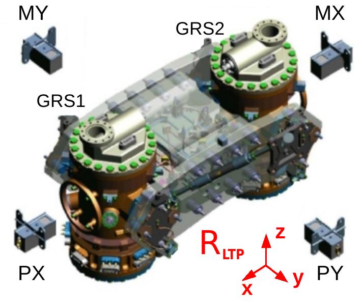
Figure 1: Sketch of the position of the four 3-axis magnetometers placed on board LPF (MX, MY, PX and PY) with respect to the gravitational reference sensors (GRS1 and GRS2) enclosing the two LPF TMs. The magnetometers were arranged in a cross-shaped configuration. MX and PX were placed at the edges of the arm joining the TM centers ($x$ direction) where the negative (M) and the positive (P) sides are meant with respect to the middle point between the two GRSs, respectively. Similarly, MY and PY were placed at the edges of the second arm ($y$ direction) where M and P have the same meaning as for the $x$-axis. The $z$-axis was chosen to complete the right-handed tern of the LTP reference frame, $\boldsymbol{\mathrm{R}}_{\mathrm{LTP}}$.

Parameter	Value
Field range	$\pm 60\ \mathrm{\mu T}$
Temperature coefficient	$1.2\,\mathrm{nT\,K^{-1}}$
Noise density	$<\!100\ \mathrm{pT\,Hz^{-1/2}}\,@\,1\mathrm{Hz}$
Linearity	$0.015\%$
Sensitivity	$166.7\ \mathrm{\mu V\,nT^{-1}}$
Offset voltage	$25\ \mathrm{mV}$ ($150\ \mathrm{nT}$)
Operating temperature	$-55\ \mathrm{{}^{\circ}C}$ to $+85\ \mathrm{{}^{\circ}C}$
Susceptibility	$\pm 20\,\mathrm{nT}$ with $0.5\ \mathrm{mT}$

Table 1: LPF magnetometer characteristics (Mateos, 2015).

The magnetic subsystem, including the four magnetometers and the acquisition electronics, was tested before the mission launch at the Universidad Politecnica de Madrid (Mateos, 2015). The calibration of the magnetometers was carried out with a 3-D Helmholtz coil (Beravs et al., 2014). By denoting with $\mathbf{B}^{\mathrm{raw}}_{m}[t]$ the raw magnetic field measurements of each magnetometer:

$$\displaystyle\mathbf{B}^{\mathrm{raw}}_{m}[t] = \mathrm{B}^{\mathrm{raw}}_{x}[t]\,\hat{x}+\mathrm{B}^{\mathrm{raw}}_{y}[t]\,\hat{y}+\mathrm{B}^{\mathrm{raw}}_{z}[t]\,\hat{z},$$ (1)

where $m$ ranges from $1$ to $4$ to indicate the four magnetometers MX, MY, PX and PY, respectively (Fig. 1). This calibration procedure allowed us to determine for each magnetic field component of individual instruments the parameters associated with gain, mis-alignment and bias. The parameters relative to the gain and to the axis mis-alignment fill two $3\times 3$ matrices: $\mathbf{s}_{m}$ and $\mathbf{T}_{m}$, respectively. Finally, the measurement offset is represented by a $3\times 1$ vector $\mathbf{b}_{m}$ as indicated below:

$$\displaystyle\mathbf{B}^{\mathrm{MAG}}_{m}[t] = \mathbf{s}_{m}\,\mathbf{T}_{m}\,\mathbf{B}^{\mathrm{raw}}_{m}[t]+\mathbf{b}_{m},$$ (2)

where $\mathbf{B}^{\mathrm{MAG}}_{m}[t]$ indicates the calibrated magnetic field measurements.

3 LPF SPACECRAFT MAGNETIC FIELD

The LPF magnetometer calibrated datasets were sampled at 2$\times$10^-1 Hz and downsampled at $3\times 10^{-4}\,\mathrm{Hz}$. Aliasing was prevented by applying a first-order bidirectional low-pass filter. The intensity of the magnetic field measured by MX, MY, PX and PY magnetometers during the LPF mission are shown in Figure 2. Observations varied by almost a factor of two between $700\,\mathrm{nT}$ and about $1300\,\mathrm{nT}$. The MX, MY and PX magnetometer recorded magnetic field values ($\mathbf{B}_{\mathrm{MX}}^{\mathrm{MAG}}$, $\mathbf{B}_{\mathrm{MY}}^{\mathrm{MAG}}$ and $\mathbf{B}_{\mathrm{PX}}^{\mathrm{MAG}}$, respectively) ranging between $800\,\mathrm{nT}$ and $1300\,\mathrm{nT}$ with sudden variations between different magnetic field intensities. Conversely, the PY magnetometer recorded stable values of the magnetic field around $700\,\mathrm{nT}$ during the whole mission lifetime ($\mathbf{B}_{\mathrm{PY}}^{\mathrm{MAG}}$). Magnetic field patterns and sudden changes were not ascribable to the IMF that was observed to present typical values in the $1-25\,\mathrm{nT}$ range (Armano et al., 2019b). In general, the magnetometers hosted on board the LPF S/C sensed a larger noise along the three cartesian axes with respect to the Magnetic Field Investigation (MFI) instrument hosted on board the Wind mission also orbiting around L1 (Lepping et al., 1995) during the same period of LPF. Despite that, the approach presented here allows us to disentangle the IMF from the magnetic field generated on board the LPF S/C.

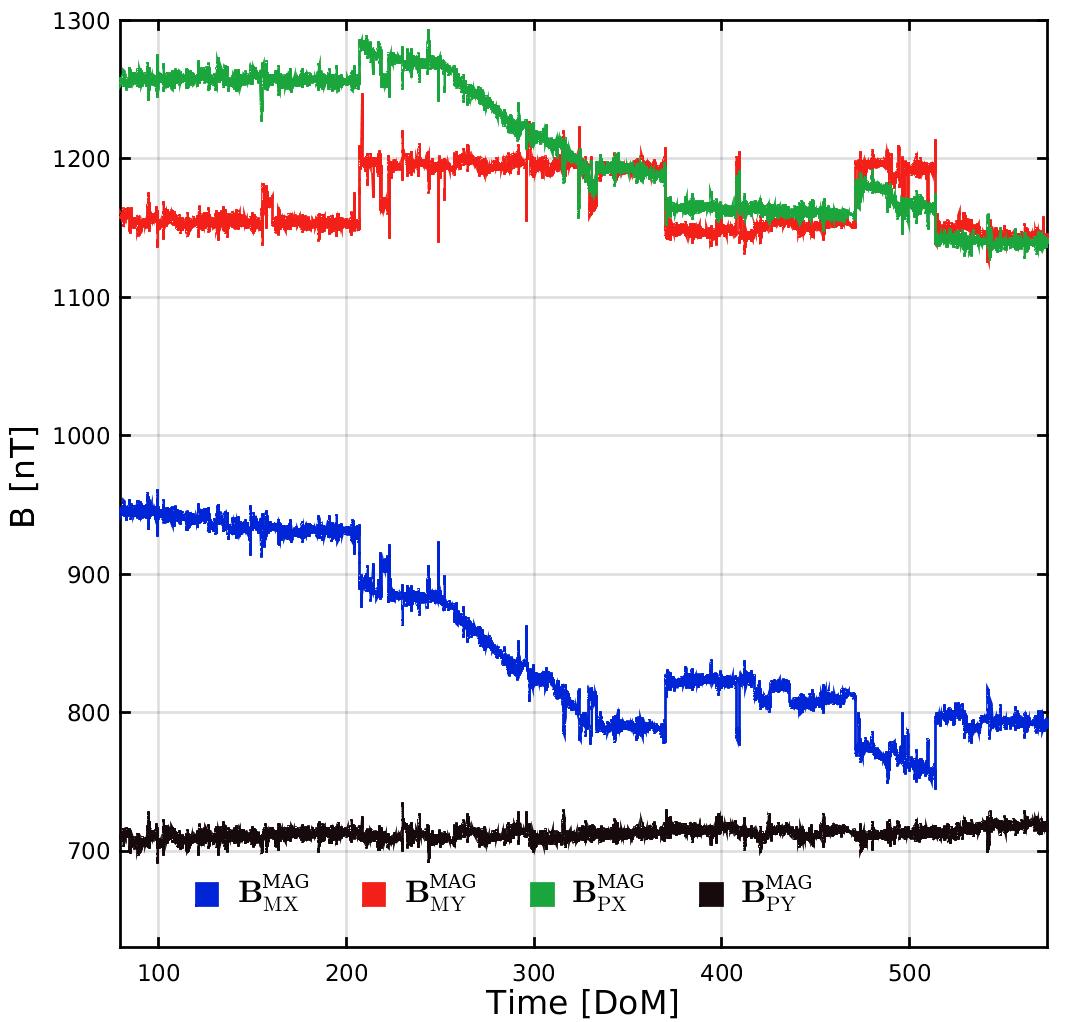
Figure 2: Magnetic field intensities recorded by the four LPF 3-axis fluxgate magnetometers during the time the S/C was orbiting around the Lagrange point L1 from February 16, 2016 through June 30, 2017. Datasets were sampled at $2\times 10^{-1}\,\mathrm{Hz}$ and downsampled at $3\times 10^{-4}\,\mathrm{Hz}$. Time is indicated in days of mission (DoM) after the LPF launch (4:04 UTC, December 3, 2015).

The power spectral densities (PSDs) of magnetic field measurements carried out with LPF during the whole mission operation period are reported in Figure 3. In the same figure the PSDs of the IMF measurements gathered with MFI are reported for comparison. It can be observed that the onboard noise overcomes that of interplanetary origin at low frequencies while it appears consistent with it above $10^{-5}\,\mathbf{Hz}$.

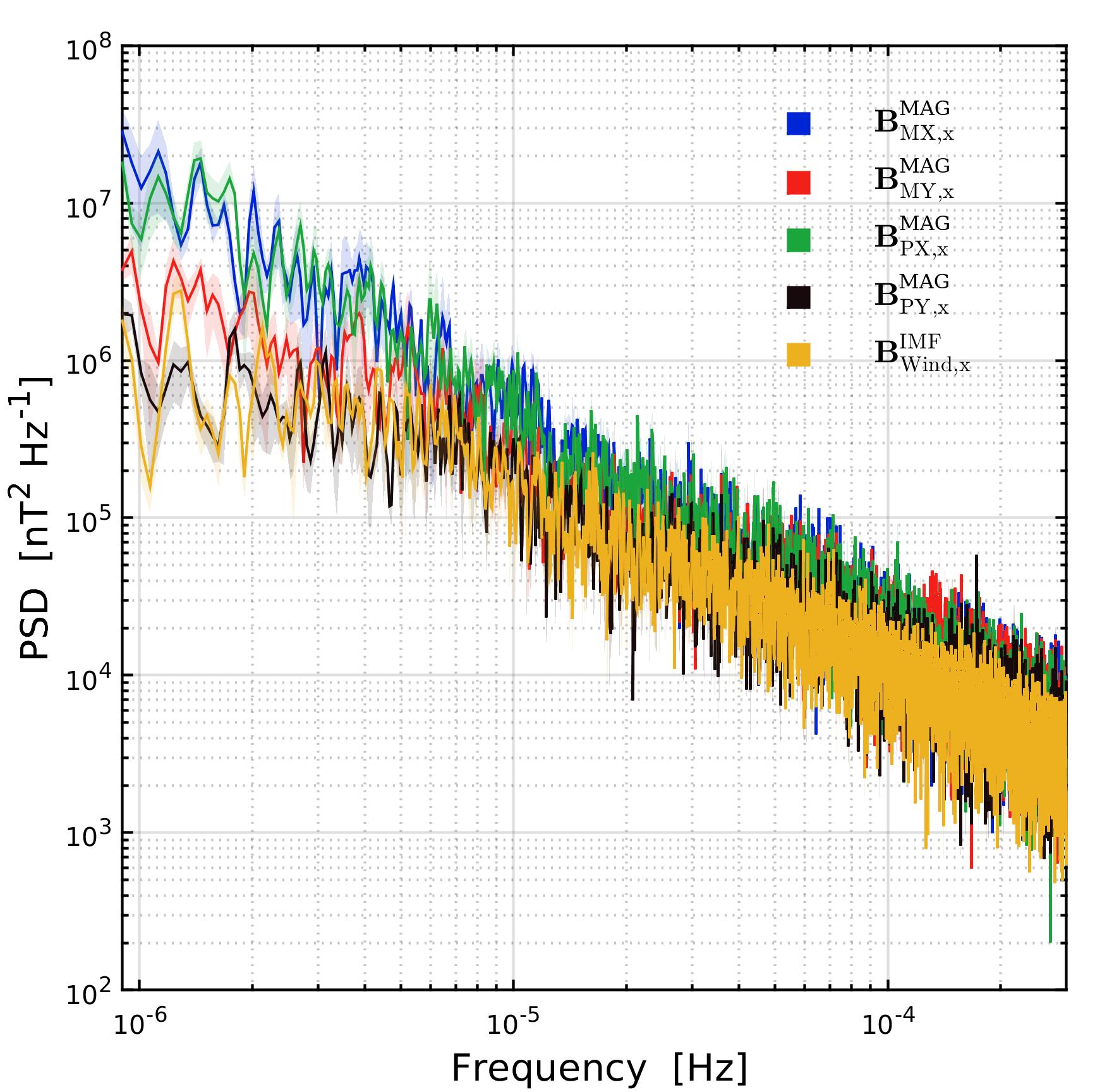
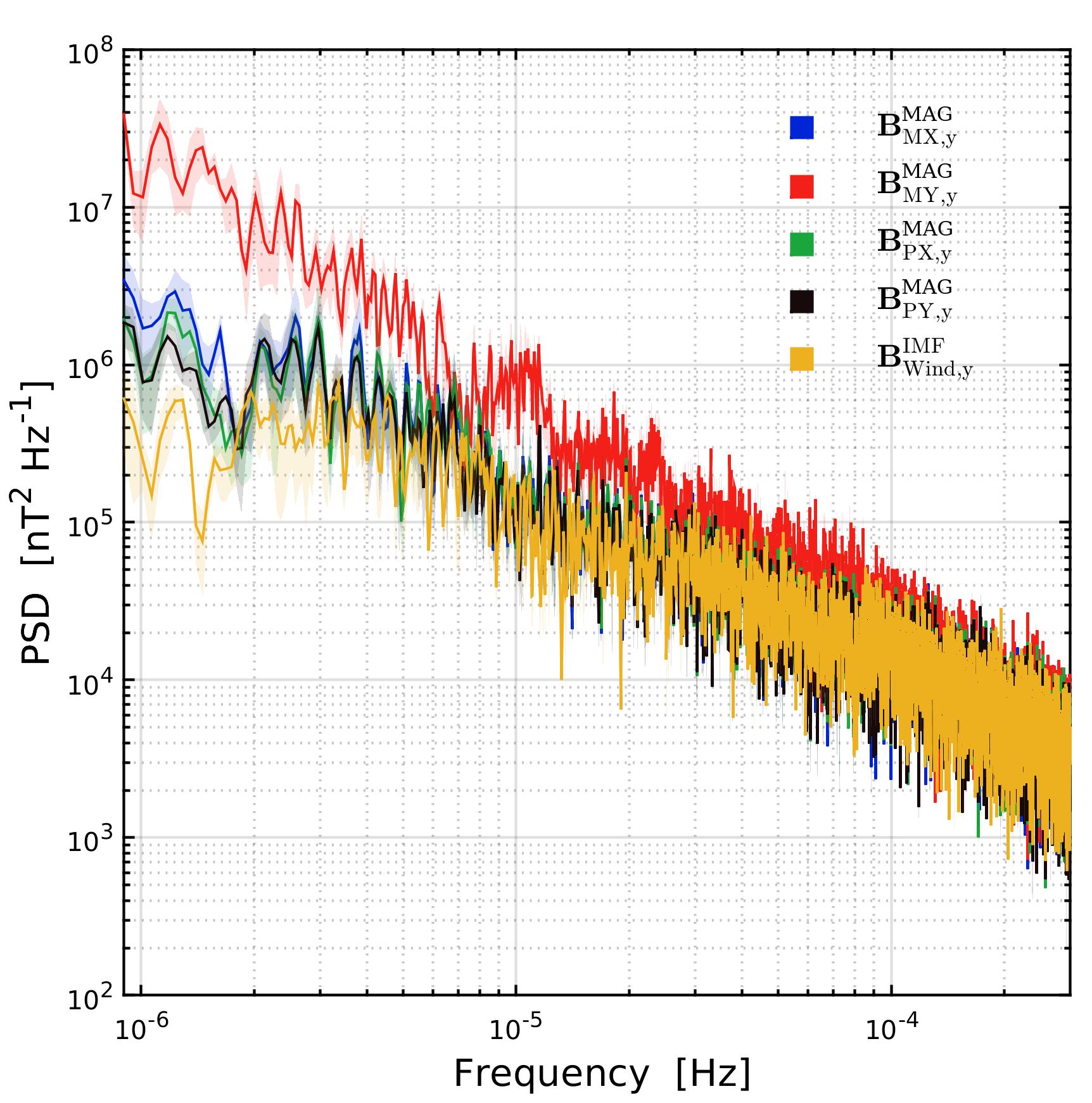
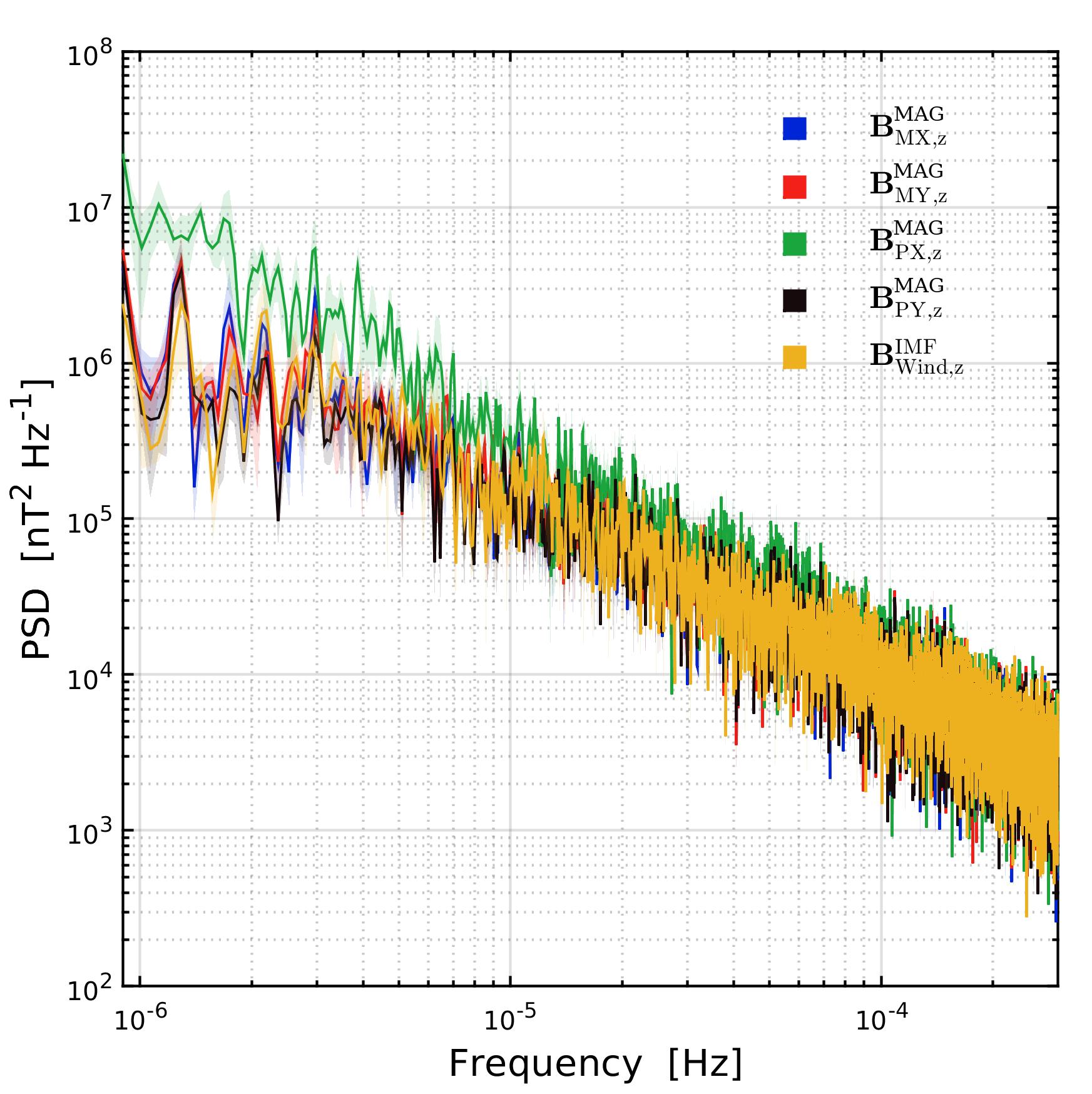
Figure 3: PSDs of LPF and Wind 3-axis magnetometer simultaneous measurements (from February 20, 2016 through June 21, 2017). All measurements were reported in the $\boldsymbol{\mathrm{R}}_{\mathrm{LTP}}$ reference frame for proper comparison.

4 PARAMETERIZATION OF THE MAGNETIC FIELD MEASUREMENTS GATHERED WITH LPF

The timeseries of the calibrated magnetic field measurements gathered on-board LPF have been parameterized as follows:

$$\mathbf{B}^{\mathrm{LPF}}_{m}[t]=\mathbf{B}^{\mathrm{EW}}_{m}[t]+\mathbf{B}^{\mathrm{ED}}_{m}[t]+\mathbf{B}^{\mathrm{M}}_{m}[t]+\mathbf{B}^{\mathrm{IMF}}_{m}[t]+\mathbf{v}^{c}_{m}[t]\ .$$ (3)

In the above equation the magnetic field measured on board the LPF S/C is considered to consist of different contributions generated by the main currents flowing through wiring and electronics in the satellite ($\mathbf{B}^{\mathrm{EW}}_{m}[t]$ and $\mathbf{B}^{\mathrm{ED}}_{m}[t]$, respectively), by the magnetized materials ($\mathbf{B}^{\mathrm{M}}_{m}[t]$) and by the IMF ($\mathbf{B}^{\mathrm{IMF}}_{m}[t]$). Finally, $\mathbf{v}^{c}_{m}[t]$ represents the residue. In the case the considered contributions to the LPF magnetic field observations are not overcome by other neglected components, the residue is expected to be negligible and mainly associated with the measurement noise.

No measurement correction due to temperature variations were considered. As a matter of fact, for more than 500 days after the mission launch, the temperature remained nearly constant around a typical value of $297.15\pm 0.75\,\mathrm{K}$ in the LPF S/C (Armano et al., 2019). This temperature variation corresponded to a magnetic field offset smaller than $0.9\,\mathrm{nT}$ (Tab. 1). Seldom during the S/C commissioning phase and in particular for a period of 20 days after April 29, 2017 (DoM 513), the temperature was purposely maintained between $281\,\mathrm{K}$ and $285\,\mathrm{K}$. Magnetic field measurements gathered during these intervals of time are shown in the following but excluded from the analysis.

4.1 Magnetic field generated by wiring and electronics on board the LPF spacecraft

The main contribution to the magnetic field measured with the MX, MY, PX and PY magnetometers in the LPF S/C is associated with currents of $10-20\,\mathrm{A}$ flowing through the main satellite and solar array buses ($I_{bus}$ and $I_{sar}$, respectively). One secondary bus ($I_{aux,A}$) distributing a current smaller than $1\,\mathrm{A}$ was also found to play an important role. Figure 4 shows the timeseries of the currents flowing in the buses indicated above during the mission operations.

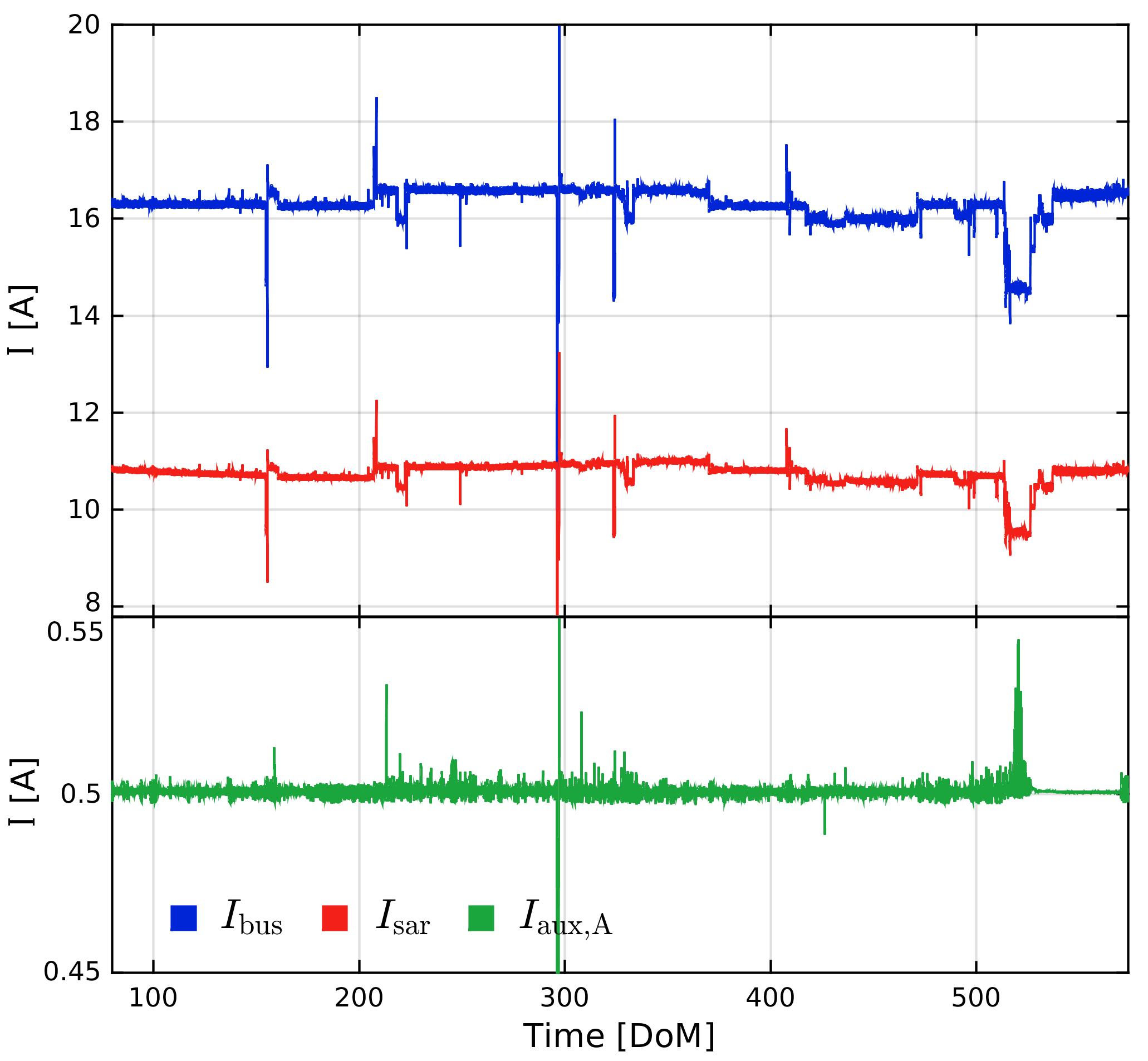
Figure 4: LPF main bus current ($I_{bus}$), solar array bus current ($I_{sar}$) and auxiliary power supply A current ($I_{aux,A}$) during the LPF mission operations from February 16, 2016 through June 30, 2017. At DoM near 300 an isolated overload is observed. Data in the corresponding interval of time have not been included in this analysis.

As an example, the correlated trend of the magnetic field measured by the MY magnetometer along the LTP $y$-axis and the main LPF current bus trend is shown in Figure 5. The IMF intensity shows both hourly variability and sudden jumps associated with the bus current changes.

Figure 5: LPF magnetic field measured by the MY magnetometer along the LTP $y$-axis (blue) and main bus current (red). The two physical quantities appear correlated and show common sudden changes.

The magnetic field components generated by the circuitry in each measurement point are observed along the axes of the $m$-th magnetometer in the $\boldsymbol{\mathrm{R}}_{\mathrm{LTP}}$ reference frame. At the magnetometer locations, each current bus produces a magnetic field proportional to the current flowing through the circuit that can be estimated with the Biot-Savart equation. As a result, the sensed magnetic field change is linearly proportional to the current change in the circuitry.

These considerations apply to the magnetic field generated by both wiring and electronics. With respect to the magnetic field generated by the electronics, LPF hosted an unregulated power conditioning and distribution unit (PCDU) (Soto et al., 2008) which showed a nearly constant power conversion efficiency, $\eta$, of 92.5% as it is shown in Figure 6. The main supply bus voltage was stabilized very efficiently at $V_{\mathrm{bus}}=27.903\pm 0.002\,\mathrm{V}$ by a Li-Ion battery which, due to a constant solar illumination, was handled at a fix charge/discharge point. Sudden changes of the power conversion efficiency and current variations were observed during electronics configuration switches only. Table 2 reports the complex changes of electronics configurations during the mission operations. The S/C was driven by the drag-free attitude control system (DFACS) or by the disturbance reduction system (DRS). Both these attitude control systems were used to command with forces and torques the S/C and the two proof TMs (Armano et al., 2016). The DFACS controlled a set of cold-gas thrusters (Morris and Edwards, 2013) and the electronics for the TM electrostatic actuation. The DRS utilized a distinct control scheme implemented by a dedicated on-board computer with electronics and a second set of $8$ colloidal micro-newton thrusters (CMNTs) (Anderson et al., 2018).

During time periods indicated by “DFACS+”, the DRS related subsystems were left switched on, even when the actuation was assigned to the DFACS. For instance, this configuration was applied during the months of July and August 2016. Analogously, the periods indicated by “DRS+” were those associated with actuation assigned to the DRS with the DFACS powered on.

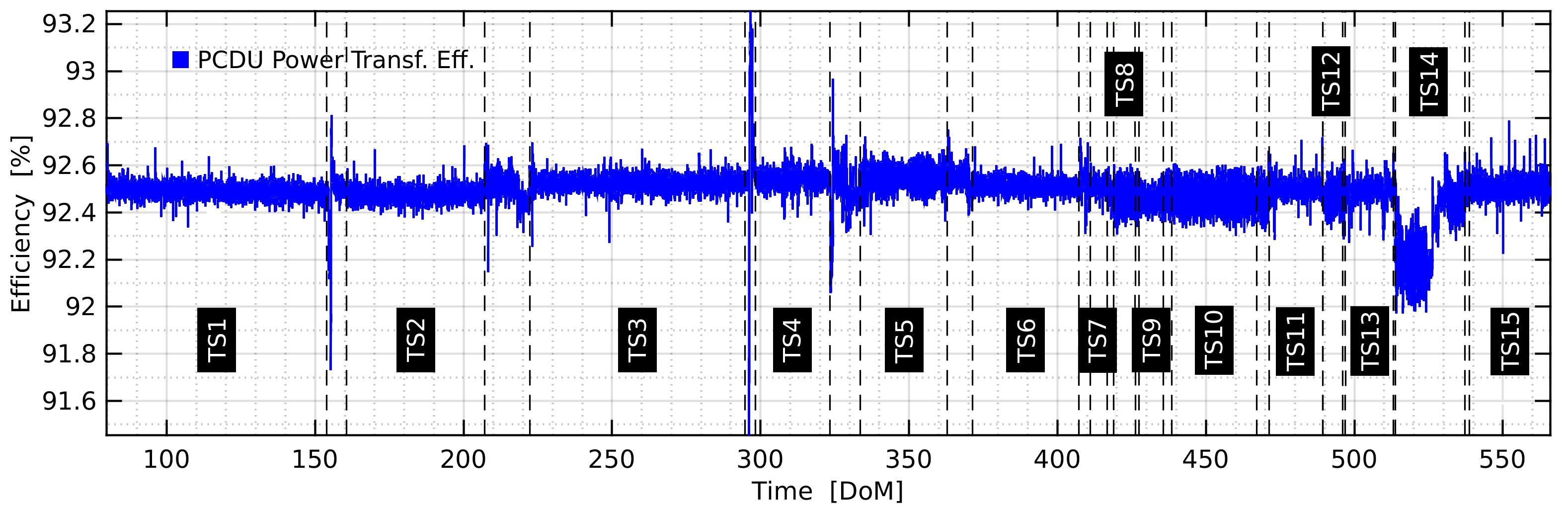
Figure 6: PCDU power transfer efficiency, $\eta[t]$.

The timespans were selected on the basis of the electronic switches, the current bus trends and the power transfer efficiency $\eta[t]$ in order to select proper magnetic field pattern changes (Fig. 2).

Timespan	Confs	Start Time	Stop Time	Duration
		[UTC]	[UTC]	[Days]
1	DFACS	2016-02-20, 22:20	2016-05-04, 23:45	74
2	DFACS	2016-05-11, 16:35	2016-06-27, 06:00	46
3	DRS	2016-07-12, 09:55	2016-09-23, 00:05	72
4	DRS	2016-09-26, 10:00	2016-10-21, 16:40	25
5	DFACS+	2016-10-31, 16:35	2016-12-07, 03:35	36
6	DFACS+	2016-12-08, 13:45	2017-01-13, 10:00	35
7	DFACS+	2017-01-17, 06:30	2017-01-22, 23:45	5
8	DFACS+	2017-01-25, 00:45	2017-02-01, 11:45	7
9	DFACS+	2017-02-02, 14:15	2017-02-10, 19:55	8
10	DFACS+	2017-02-13, 17:35	2017-03-14, 06:00	28
11	DRS+	2017-03-18, 10:00	2017-04-05, 10:50	18
12	DFACS+	2017-04-05, 12:55	2017-04-12, 04:05	6
13	DRS+	2017-04-13, 02:15	2017-04-29, 07:30	16
14	DFACS+	2017-04-30, 00:05	2017-05-23, 07:30	23
15	DFACS+	2017-05-24, 20:25	2017-06-21, 20:00	27

Table 2: LPF electronics configuration during different time intervals.

In conclusion, according to the Biot-Savart law and the superposition principle (Yu et al., 2013), the magnetic field intensity produced at each magnetometer position ($m$) by wiring and electronics is empirically parameterized as indicated in the following equation:

$$\displaystyle\mathbf{B}^{\mathrm{EM}}_{m}[t] = \mathbf{B}^{\mathrm{EW}}_{m}[t]+\mathbf{B}^{\mathrm{ED}}_{m}[t]=$$ (4)

$$= \sum_{j=1}^{3}\frac{\mu_{0}}{4\pi}\int_{\mathcal{C}_{j}}\frac{I_{j}[t]}{r_{m,j}^{2}}d\mathbf{l}_{j}\times\mathbf{u}_{m,j}=$$

$$= \sum_{j=1}^{3}\,\mathbf{a}_{m,j}\,I_{j}[t]$$

where $d\mathbf{l}_{j}$ represents the infinitesimal current element along the $\mathcal{C}_{j}$ integration path associated with the $j$-th bus; $r_{m,j}$ indicates the distance of each $d\mathbf{l}_{j}$ current segment of each current bus from the $m$-th position of each magnetometer and $\mathbf{u}_{m,j}$ is the unit vector associated with $\mathbf{r}_{m,j}$ indicating the distance from the bus element to the point where the field is calculated. The $\mathbf{a}_{m,j}$ parameters allow to account for the magnetic field generated by the $j$-th bus current, $I_{j}[t]$. These parameters are estimated in Section V.

4.2 LPF magnetic field generated by magnetized materials

Two distinct independent micro propulsion systems were hosted on board the LPF S/C: cold-gas micro propulsion thrusters, as inherited from the Gaia mission (Scharlemann et al., 2011), and $8$ CMNTs developed by Busek and managed by NASA at the Jet Propulsion Laboratory (Ziemer et al., 2006) which were part of the DRS. The DRS included four subsystems: the Integrated Avionics Unit (IAU), two clusters of four CMNTs each, the Dynamic Control Software (DCS) and the Flight Software (FSW). CMNTs were commanded by applying an electric potential to a charged liquid in order to emit a stream of droplets for the thrust. During the mission, a major contribution to the magnetic field disturbance was found to be strongly correlated with the CMNT fuel mass ejection (Fig. 7).

Figure 7: Total CMNT fuel mass ejected and on-board induction magnetic field timeseries $\mathbf{B}^{\mathrm{MAG}}_{\mathrm{MX},x}[t]$ (in blue and red, respectively) recorded by the MX magnetometer along the LTP $x$-axis.

A magnetized assembly pushes out the propellant by moving out from the magnetometers and generating a slowly decreasing magnetic field (Armano et al., 2020). This decrease is mostly sensed by the MX and PX magnetometers along the LTP $x$-axis. On the basis of the correlated behavior between the on-board magnetic field variation and the fuel mass ejection timeseries, the contribution to the on-board magnetic field arising from the CMNT tank moving assemblies is modeled as follows:

$$\mathbf{B}_{m}^{\mathrm{M}}[t]=\mathbf{l}_{m}\ M[t]$$ (5)

where $M[t]=\sum_{i=1}^{8}{C\!M\!N\!T}_{i}[t]$ accounts for the fuel mass loss obtained by summing up the fuel mass quantity ejected from the CMNTs (Fig. 7). In Equation 5, $\mathbf{l}_{m}$ is a parameter tuned via numerical fitting (see Section 5.1) and expressed in units of $\mathrm{nT\,kg^{-1}}$.

5 Interplanetary magnetic field monitoring with LISA Pathfinder

5.1 Data analysis

The magnetic field measured on board the LPF S/C expressed in Equation 3 can be now parameterized as follows:

$$\mathbf{B}^{\mathrm{LPF}}_{m}[t] = \mathbf{B}^{\mathrm{EM}}_{m}[t]+\mathbf{B}^{\mathrm{M}}_{m}[t]+\mathbf{B}^{\mathrm{IMF}}_{m}[t]+\mathbf{v}^{c}_{m}[t]$$ (6)

$$\cong \sum_{j=1}^{3}\mathbf{a}_{j,m}I_{j}[t]+\mathbf{l}_{m}\ M[t]+\mathbf{B}^{\mathrm{IMF}}_{m}[t]+\mathbf{v}^{c}_{m}[t]\ .$$

From the above equation, it is possible to estimate the IMF component in the time domain. The same equation can be written in the frequency domain in order to remove the colored noise from the data. In the frequency domain each term is indicated with the tilde symbol and the IMF can be expressed as indicated below:

$$\mathbf{\tilde{B}}^{\mathrm{IMF}}_{m}[f] \cong \mathbf{\tilde{B}}^{\mathrm{LPF}}_{m}[f]-\sum_{j=1}^{3}\mathbf{a}_{j,m}\tilde{I}_{j}[f]-\mathbf{l}_{m}\ \tilde{M}[f]+\mathbf{\tilde{v}}^{c}_{m}[f]\,$$ (7)

where $\mathbf{\tilde{v}}^{c}_{m}[f]$ is expected to be the overall noise amplitude in case all the main components of the magnetic field have been taken into account. The LPF Data Analysis toolbox (LTPDA, publicly available at https://www.elisascience.org/ltpda/) is a toolbox implemented in Matlab (http://www.mathworks.com) and was specifically developed for the analysis of the LPF mission data (Antonucci et al., 2011). A Markov Chain Monte Carlo (MCMC) algorithm was used to estimate the posterior distribution of the model parameters on the basis of the data timeseries provided in input (Vitale et al., 2014). The parameter distribution $\mathrm{\hat{\theta}}$ was obtained with an iterative least square error estimate after the PSDs of $\tilde{I}_{j}[f]$ and $\tilde{M}[f]$ were calculated from the equivalent timeseries in the time domain. By indicating with $\theta_{m}$ the column vector of the input parameters:

$$\boldsymbol{\mathrm{\theta}}_{m}=\left[\mathbf{a}_{m,j}\,,\,\mathbf{l}_{m}\right]^{T}$$ (8)

the IMF has been estimated by minimizing the residue among collected data and empirical modelization of the LPF S/C on-board magnetic field, as follows:

$$\boldsymbol{\mathrm{\hat{\theta}}}_{m} \simeq \operatorname*{arg\,min}_{\theta_{m}}\left|\mathbf{\tilde{B}}^{\mathrm{MAG}}_{m}(\theta_{m})[f]-\mathbf{\tilde{B}}^{\mathrm{LPF}}_{m}(\theta_{m})[f]\right|\,.$$ (9)

Separate sets of parameters were estimated for each magnetometer and for each time segment listed in Table 2. The fitting program returned the IMF intensity values in the range $1-25\,\mathrm{nT}$ in line with the observations gathered by the Wind experiment during the LPF mission lifetime. Parameter estimates and corresponding uncertainties are reported in Tables 3, 4, 5 and 6. As it was recalled in Section 4, the parameters associated with TS13 and TS14 timespans were ignored because of an abrupt fall of the temperature on board the S/C.

$\begin{array}[]{|c|c|c|c|c|c|}\hline\cr\begin{array}[]{c}\\ \mathbf{MAG1}\\ \mathbf{Coefficients}\end{array}&\mathbf{Axis}&\mathbf{a_{1}}\mathrm{[\mathrm{nT\,nA^{-1}}]}&\mathbf{a_{2}}\mathrm{[\mathrm{nT\,nA^{-1}}]}&\mathbf{a_{3}}\mathrm{[\mathrm{nT\,nA^{-1}}]}&\mathbf{l}\,\mathrm{[\mathrm{nT\,kg^{-1}}]}\\ &&\begin{array}[]{cccc}value&\pm&error&(\%)\\ \end{array}&\begin{array}[]{cccc}value&\pm&error&(\%)\\ \end{array}&\begin{array}[]{cccc}value&\pm&error&(\%)\\ \end{array}&\begin{array}[]{cccc}value&\pm&error&(\%)\\ \end{array}\\ \hline\cr\begin{array}[]{c}\\ \mathbf{TS1}\\ \mathrm{(74\,days)}\end{array}&\begin{array}[]{c}x\\ y\\ z\\ \end{array}&\begin{array}[]{cccc}-69.638&\pm&5.870&(8\%)\\ \leavevmode\nobreak\ 75.271&\pm&5.682&(7\%)\\ \leavevmode\nobreak\ 35.670&\pm&7.591&(21\%)\\ \end{array}&\begin{array}[]{cccc}\leavevmode\nobreak\ 108.11&\pm&8.06&(7\%)\\ -126.72&\pm&8.49&(7\%)\\ -36.602&\pm&10.360&(28\%)\\ \end{array}&\begin{array}[]{cccc}\leavevmode\nobreak\ 1997.0&\pm&86.6&(4\%)\\ -812.57&\pm&67.51&(8\%)\\ -240.66&\pm&97.07&(40\%)\\ \end{array}&\\ \hline\cr\begin{array}[]{c}\\ \mathbf{TS2}\\ \mathrm{(46\,days)}\end{array}&\begin{array}[]{c}x\\ y\\ z\\ \end{array}&\begin{array}[]{cccc}\leavevmode\nobreak\ 65.043&\pm&24.560&(38\%)\\ \nobreak\leavevmode\hfil&&&\\ \leavevmode\nobreak\ 15.921&\pm&2.684&(17\%)\\ \end{array}&\begin{array}[]{cccc}-80.400&\pm&36.740&(46\%)\\ \nobreak\leavevmode\hfil&&&\\ \nobreak\leavevmode\hfil&&&\\ \end{array}&\begin{array}[]{cccc}\leavevmode\nobreak\ 1545.4&\pm&103.1&(15\%)\\ -1134.6&\pm&0.7&(0\%)\\ -403.53&\pm&110.80&(27\%)\\ \end{array}&\\ \hline\cr\begin{array}[]{c}\\ \mathbf{TS3}\\ \mathrm{(72\,days)}\end{array}&\begin{array}[]{c}x\\ y\\ z\\ \end{array}&\begin{array}[]{cccc}\nobreak\leavevmode\hfil&&&\\ -53.988&\pm&19.020&(35\%)\\ \nobreak\leavevmode\hfil&&&\\ \end{array}&\begin{array}[]{cccc}-41.448&\pm&1.352&(3\%)\\ \leavevmode\nobreak\ 82.558&\pm&28.040&(34\%)\\ \nobreak\leavevmode\hfil&&&\\ \end{array}&\begin{array}[]{cccc}\leavevmode\nobreak\ 3086.1&\pm&36.8&(1\%)\\ -1127.5&\pm&66.7&(6\%)\\ \leavevmode\nobreak\ 242.26&\pm&1.97&(1\%)\\ \end{array}&\begin{array}[]{cccc}\leavevmode\nobreak\ 343.64&\pm&5.57&(2\%)\\ \nobreak\leavevmode\hfil&&&\\ \leavevmode\nobreak\ 73.302&\pm&8.083&(11\%)\\ \end{array}\\ \hline\cr\begin{array}[]{c}\\ \mathbf{TS4}\\ \mathrm{(25\,days)}\end{array}&\begin{array}[]{c}x\\ y\\ z\\ \end{array}&\begin{array}[]{cccc}-47.867&\pm&26.260&(55\%)\\ \nobreak\leavevmode\hfil&&&\\ \nobreak\leavevmode\hfil&&&\\ \end{array}&\begin{array}[]{cccc}\leavevmode\nobreak\ 89.593&\pm&38.550&(43\%)\\ \nobreak\leavevmode\hfil&&&\\ \nobreak\leavevmode\hfil&&&\\ \end{array}&\begin{array}[]{cccc}\leavevmode\nobreak\ 1471.5&\pm&91.1&(6\%)\\ -1099.3&\pm&1.4&(0\%)\\ \leavevmode\nobreak\ 260.65&\pm&1.5&(1\%)\\ \end{array}&\\ \hline\cr\begin{array}[]{c}\\ \mathbf{TS5}\\ \mathrm{(36\,days)}\end{array}&\begin{array}[]{c}x\\ y\\ z\\ \end{array}&\begin{array}[]{cccc}-25.582&\pm&10.990&(43\%)\\ -25.882&\pm&10.700&(41\%)\\ \nobreak\leavevmode\hfil&&&\\ \end{array}&\begin{array}[]{cccc}\leavevmode\nobreak\ 53.523&\pm&15.940&(30\%)\\ \leavevmode\nobreak\ 31.480&\pm&15.830&(52\%)\\ \nobreak\leavevmode\hfil&&&\\ \end{array}&\begin{array}[]{cccc}\leavevmode\nobreak\ 1525.4&\pm&100.8&(7\%)\\ -867.43&\pm&101.7&(12\%)\\ \leavevmode\nobreak\ 278.89&\pm&0.63&(0\%)\\ \end{array}&\\ \hline\cr\begin{array}[]{c}\\ \mathbf{TS6}\\ \mathrm{(35\,days)}\end{array}&\begin{array}[]{c}x\\ y\\ z\\ \end{array}&\begin{array}[]{cccc}\nobreak\leavevmode\hfil&&&\\ -14.609&\pm&4.214&(29\%)\\ \nobreak\leavevmode\hfil&&&\\ \end{array}&\begin{array}[]{cccc}\nobreak\leavevmode\hfil&&&\\ \nobreak\leavevmode\hfil&&&\\ \nobreak\leavevmode\hfil&&&\\ \end{array}&\begin{array}[]{cccc}\leavevmode\nobreak\ 1767.0&\pm&0.8&(0\%)\\ -474.09&\pm&173.90&(37\%)\\ \leavevmode\nobreak\ 302.27&\pm&0.89&(0\%)\\ \end{array}&\\ \hline\cr\begin{array}[]{c}\\ \mathbf{TS7}\\ \mathrm{(5\,days)}\end{array}&\begin{array}[]{c}x\\ y\\ z\\ \end{array}&\begin{array}[]{cccc}\nobreak\leavevmode\hfil&&&\\ \nobreak\leavevmode\hfil&&&\\ \nobreak\leavevmode\hfil&&&\\ \end{array}&\begin{array}[]{cccc}\nobreak\leavevmode\hfil&&&\\ \nobreak\leavevmode\hfil&&&\\ \nobreak\leavevmode\hfil&&&\\ \end{array}&\begin{array}[]{cccc}\leavevmode\nobreak\ 1766.7&\pm&2.5&(1\%)\\ -1088.8&\pm&4.1&(0\%)\\ \leavevmode\nobreak\ 300.39&\pm&2.98&(1\%)\\ \end{array}&\\ \hline\cr\begin{array}[]{c}\\ \mathbf{TS8}\\ \mathrm{(7\,days)}\end{array}&\begin{array}[]{c}x\\ y\\ z\\ \end{array}&\begin{array}[]{cccc}\nobreak\leavevmode\hfil&&&\\ \nobreak\leavevmode\hfil&&&\\ \nobreak\leavevmode\hfil&&&\\ \end{array}&\begin{array}[]{cccc}\nobreak\leavevmode\hfil&&&\\ \nobreak\leavevmode\hfil&&&\\ \nobreak\leavevmode\hfil&&&\\ \end{array}&\begin{array}[]{cccc}\leavevmode\nobreak\ 1730.6&\pm&1.5&(0\%)\\ -1070.8&\pm&1.9&(0\%)\\ \leavevmode\nobreak\ 313.74&\pm&2.40&(1\%)\\ \end{array}&\\ \hline\cr\begin{array}[]{c}\\ \mathbf{TS9}\\ \mathrm{(8\,days)}\end{array}&\begin{array}[]{c}x\\ y\\ z\\ \end{array}&\begin{array}[]{cccc}\leavevmode\nobreak\ 32.841&\pm&4.103&(12\%)\\ \nobreak\leavevmode\hfil&&&\\ \nobreak\leavevmode\hfil&&&\\ \end{array}&\begin{array}[]{cccc}\nobreak\leavevmode\hfil&&&\\ \nobreak\leavevmode\hfil&&&\\ \nobreak\leavevmode\hfil&&&\\ \end{array}&\begin{array}[]{cccc}\leavevmode\nobreak\ 723.90&\pm&165.50&(23\%)\\ -1088.4&\pm&1.0&(0\%)\\ \leavevmode\nobreak\ 309.93&\pm&0.89&(0\%)\\ \end{array}&\\ \hline\cr\begin{array}[]{c}\\ \mathbf{TS10}\\ \mathrm{(28\,days)}\end{array}&\begin{array}[]{c}x\\ y\\ z\\ \end{array}&\begin{array}[]{cccc}\leavevmode\nobreak\ 84.19&\pm&18.34&(22\%)\\ \nobreak\leavevmode\hfil&&&\\ \nobreak\leavevmode\hfil&&&\\ \end{array}&\begin{array}[]{cccc}-113.01&\pm&26.52&(23\%)\\ \nobreak\leavevmode\hfil&&&\\ \nobreak\leavevmode\hfil&&&\\ \end{array}&\begin{array}[]{cccc}\leavevmode\nobreak\ 1637.6&\pm&155.2&(9\%)\\ -1077.6&\pm&0.7&(0\%)\\ \leavevmode\nobreak\ 318.52&\pm&0.84&(0\%)\\ \end{array}&\\ \hline\cr\begin{array}[]{c}\\ \mathbf{TS11}\\ \mathrm{(18\,days)}\end{array}&\begin{array}[]{c}x\\ y\\ z\\ \end{array}&\begin{array}[]{cccc}\leavevmode\nobreak\ 30.807&\pm&20.480&(66\%)\\ \nobreak\leavevmode\hfil&&&\\ \leavevmode\nobreak\ 76.224&\pm&27.610&(36\%)\\ \end{array}&\begin{array}[]{cccc}-59.847&\pm&30.920&(52\%)\\ \nobreak\leavevmode\hfil&&&\\ -125.41&\pm&42.28&(34\%)\\ \end{array}&\begin{array}[]{cccc}\leavevmode\nobreak\ 2276.3&\pm&107.5&(5\%)\\ -1071.6&\pm&1.1&(0\%)\\ \leavevmode\nobreak\ 559.59&\pm&138.10&(25\%)\\ \end{array}&\\ \hline\cr\begin{array}[]{c}\\ \mathbf{TS12}\\ \mathrm{(6\,days)}\end{array}&\begin{array}[]{c}x\\ y\\ z\\ \end{array}&\begin{array}[]{cccc}\nobreak\leavevmode\hfil&&&\\ \nobreak\leavevmode\hfil&&&\\ \nobreak\leavevmode\hfil&&&\\ \end{array}&\begin{array}[]{cccc}\nobreak\leavevmode\hfil&&&\\ \nobreak\leavevmode\hfil&&&\\ \nobreak\leavevmode\hfil&&&\\ \end{array}&\begin{array}[]{cccc}\leavevmode\nobreak\ 1826.4&\pm&78.3&(4\%)\\ -1339.2&\pm&77.5&(17\%)\\ \nobreak\leavevmode\hfil&&&\\ \end{array}&\\ \hline\cr\begin{array}[]{c}\\ \mathbf{TS13}\\ \mathrm{(16\,days)}\end{array}&\begin{array}[]{c}x\\ y\\ z\\ \end{array}&&&&\\ \hline\cr\begin{array}[]{c}\\ \mathbf{TS14}\\ \mathrm{(23\,days)}\end{array}&\begin{array}[]{c}x\\ y\\ z\\ \end{array}&&&&\\ \hline\cr\begin{array}[]{c}\\ \mathbf{TS15}\\ \mathrm{(34\,days)}\end{array}&\begin{array}[]{c}x\\ y\\ z\\ \end{array}&\begin{array}[]{cccc}-84.556&\pm&17.160&(20\%)\\ -40.899&\pm&21.410&(52\%)\\ \nobreak\leavevmode\hfil&&&\\ \end{array}&\begin{array}[]{cccc}\leavevmode\nobreak\ 122.18&\pm&25.14&(20\%)\\ \leavevmode\nobreak\ 47.726&\pm&31.070&(65\%)\\ \nobreak\leavevmode\hfil&&&\\ \end{array}&\begin{array}[]{cccc}\leavevmode\nobreak\ 2194.5&\pm&108.5&(5\%)\\ -663.54&\pm&97.71&(7\%)\\ \leavevmode\nobreak\ 324.54&\pm&0.85&(0\%)\\ \end{array}&\\ \hline\cr\end{array}$

Table 3: MCMC parameter and parameter uncertainty estimates obtained by performing a joint fit on the measurements of the MX magnetometer. The parameters appear in Equation 7.

$\begin{array}[]{|c|c|c|c|c|c|}\hline\cr\begin{array}[]{c}\\ \mathbf{MAG2}\\ \mathbf{Coefficients}\end{array}&\mathbf{Axis}&\mathbf{a_{1}}\mathrm{[\mathrm{nT\,nA^{-1}}]}&\mathbf{a_{2}}\mathrm{[\mathrm{nT\,nA^{-1}}]}&\mathbf{a_{3}}\mathrm{[\mathrm{nT\,nA^{-1}}]}&\mathbf{l}\,\mathrm{[\mathrm{nT\,kg^{-1}}]}\\ &&\begin{array}[]{cccc}value&\pm&error&(\%)\\ \end{array}&\begin{array}[]{cccc}value&\pm&error&(\%)\\ \end{array}&\begin{array}[]{cccc}value&\pm&error&(\%)\\ \end{array}&\begin{array}[]{cccc}value&\pm&error&(\%)\\ \end{array}\\ \hline\cr\begin{array}[]{c}\\ \mathbf{TS1}\\ \mathrm{(74\,days)}\end{array}&\begin{array}[]{c}x\\ y\\ z\\ \end{array}&\begin{array}[]{cccc}-26.903&\pm&5.222&(19\%)\\ \nobreak\leavevmode\hfil&&&\\ \nobreak\leavevmode\hfil&&&\\ \end{array}&\begin{array}[]{cccc}\leavevmode\nobreak\ 32.724&\pm&7.907&(24\%)\\ \nobreak\leavevmode\hfil&&&\\ \nobreak\leavevmode\hfil&&&\\ \end{array}&\begin{array}[]{cccc}\nobreak\leavevmode\hfil&&&\\ \leavevmode\nobreak\ 2593.8&\pm&0.6&(0\%)\\ \leavevmode\nobreak\ 1339.2&\pm&0.7&(0\%)\\ \end{array}&\\ \hline\cr\begin{array}[]{c}\\ \mathbf{TS2}\\ \mathrm{(46\,days)}\end{array}&\begin{array}[]{c}x\\ y\\ z\\ \end{array}&\begin{array}[]{cccc}\nobreak\leavevmode\hfil&&&\\ \nobreak\leavevmode\hfil&&&\\ \nobreak\leavevmode\hfil&&&\\ \end{array}&\begin{array}[]{cccc}\leavevmode\nobreak\ 36.931&\pm&36.090&(99\%)\\ \nobreak\leavevmode\hfil&&&\\ \nobreak\leavevmode\hfil&&&\\ \end{array}&\begin{array}[]{cccc}-212.10&\pm&0.75&(1\%)\\ \leavevmode\nobreak\ 2587.1&\pm&0.6&(0\%)\\ \leavevmode\nobreak\ 974.16&\pm&94.70&(10\%)\\ \end{array}&\\ \hline\cr\begin{array}[]{c}\\ \mathbf{TS3}\\ \mathrm{(72\,days)}\end{array}&\begin{array}[]{c}x\\ y\\ z\\ \end{array}&\begin{array}[]{cccc}-16.675&\pm&1.560&(10\%)\\ \leavevmode\nobreak\ 238.71&\pm&30.06&(13\%)\\ \nobreak\leavevmode\hfil&&&\\ \end{array}&\begin{array}[]{cccc}\nobreak\leavevmode\hfil&&&\\ -296.12&\pm&44.96&(15\%)\\ \nobreak\leavevmode\hfil&&&\\ \end{array}&\begin{array}[]{cccc}\leavevmode\nobreak\ 464.84&\pm&65.09&(14\%)\\ \leavevmode\nobreak\ 827.64&\pm&49.48&(6\%)\\ \leavevmode\nobreak\ 983.87&\pm&0.84&(0\%)\\ \end{array}&\begin{array}[]{cccc}\leavevmode\nobreak\ 57.846&\pm&6.598&(11\%)\\ -65.990&\pm&10.370&(16\%)\\ \nobreak\leavevmode\hfil&&&\\ \end{array}\\ \hline\cr\begin{array}[]{c}\\ \mathbf{TS4}\\ \mathrm{(25\,days)}\end{array}&\begin{array}[]{c}x\\ y\\ z\\ \end{array}&\begin{array}[]{cccc}\nobreak\leavevmode\hfil&&&\\ \leavevmode\nobreak\ 119.43&\pm&23.12&(19\%)\\ \leavevmode\nobreak\ 112.37&\pm&19.57&(17\%)\\ \end{array}&\begin{array}[]{cccc}-9.1909&\pm&0.0261&(0\%)\\ -132.65&\pm&34.75&(26\%)\\ -144.67&\pm&29.64&(20\%)\\ \end{array}&\begin{array}[]{cccc}\nobreak\leavevmode\hfil&&&\\ \leavevmode\nobreak\ 1309.4&\pm&70.77&(5\%)\\ \leavevmode\nobreak\ 647.39&\pm&89.37&(14\%)\\ \end{array}&\\ \hline\cr\begin{array}[]{c}\\ \mathbf{TS5}\\ \mathrm{(36\,days)}\end{array}&\begin{array}[]{c}x\\ y\\ z\\ \end{array}&\begin{array}[]{cccc}-5.6256&\pm&0.0115&(0\%)\\ \nobreak\leavevmode\hfil&&&\\ \nobreak\leavevmode\hfil&&&\\ \end{array}&\begin{array}[]{cccc}\nobreak\leavevmode\hfil&&&\\ \leavevmode\nobreak\ 29.212&\pm&3.182&(11\%)\\ \nobreak\leavevmode\hfil&&&\\ \end{array}&\begin{array}[]{cccc}\nobreak\leavevmode\hfil&&&\\ \leavevmode\nobreak\ 1820.4&\pm&88.6&(5\%)\\ \leavevmode\nobreak\ 1359.8&\pm&0.5&(0\%)\\ \end{array}&\\ \hline\cr\begin{array}[]{c}\\ \mathbf{TS6}\\ \mathrm{(35\,days)}\end{array}&\begin{array}[]{c}x\\ y\\ z\\ \end{array}&\begin{array}[]{cccc}-95.289&\pm&42.090&(44\%)\\ \leavevmode\nobreak\ 19.384&\pm&3.460&(18\%)\\ \leavevmode\nobreak\ 8.7730&\pm&3.271&(37\%)\\ \end{array}&\begin{array}[]{cccc}\leavevmode\nobreak\ 135.09&\pm&63.32&(47\%)\\ \nobreak\leavevmode\hfil&&&\\ \nobreak\leavevmode\hfil&&&\\ \end{array}&\begin{array}[]{cccc}\leavevmode\nobreak\ 1696.1&\pm&142.7&(8\%)\\ -474.09&\pm&173.90&(37\%)\\ \leavevmode\nobreak\ 1011.6&\pm&134.9&(13\%)\\ \end{array}&\\ \hline\cr\begin{array}[]{c}\\ \mathbf{TS7}\\ \mathrm{(5\,days)}\end{array}&\begin{array}[]{c}x\\ y\\ z\\ \end{array}&\begin{array}[]{cccc}\nobreak\leavevmode\hfil&&&\\ \leavevmode\nobreak\ 307.59&\pm&95.95&(31\%)\\ \nobreak\leavevmode\hfil&&&\\ \end{array}&\begin{array}[]{cccc}\nobreak\leavevmode\hfil&&&\\ -430.86&\pm&133.70&(31\%)\\ \nobreak\leavevmode\hfil&&&\\ \end{array}&\begin{array}[]{cccc}-232.21&\pm&1.52&(1\%)\\ \leavevmode\nobreak\ 1601.0&\pm&471.4&(29\%)\\ \leavevmode\nobreak\ 1368.7&\pm&3.0&(0\%)\\ \end{array}&\\ \hline\cr\begin{array}[]{c}\\ \mathbf{TS8}\\ \mathrm{(7\,days)}\end{array}&\begin{array}[]{c}x\\ y\\ z\\ \end{array}&\begin{array}[]{cccc}\nobreak\leavevmode\hfil&&&\\ \nobreak\leavevmode\hfil&&&\\ \leavevmode\nobreak\ 62.563&\pm&43.130&(69\%)\\ \end{array}&\begin{array}[]{cccc}\nobreak\leavevmode\hfil&&&\\ \leavevmode\nobreak\ 64.123&\pm&11.620&(18\%)\\ -85.866&\pm&59.660&(69\%)\\ \end{array}&\begin{array}[]{cccc}-192.31&\pm&1.134&(1\%)\\ \leavevmode\nobreak\ 775.34&\pm&314.10&(40\%)\\ \leavevmode\nobreak\ 1166.2&\pm&231.1&(20\%)\\ \end{array}&\\ \hline\cr\begin{array}[]{c}\\ \mathbf{TS9}\\ \mathrm{(8\,days)}\end{array}&\begin{array}[]{c}x\\ y\\ z\\ \end{array}&\begin{array}[]{cccc}\nobreak\leavevmode\hfil&&&\\ \leavevmode\nobreak\ 40.555&\pm&6.551&(16\%)\\ \nobreak\leavevmode\hfil&&&\\ \end{array}&\begin{array}[]{cccc}\nobreak\leavevmode\hfil&&&\\ \nobreak\leavevmode\hfil&&&\\ \nobreak\leavevmode\hfil&&&\\ \end{array}&\begin{array}[]{cccc}-1548.4&\pm&1.3&(0\%)\\ \leavevmode\nobreak\ 869.62&\pm&263.90&(30\%)\\ \leavevmode\nobreak\ 1057.4&\pm&1.5&(0\%)\\ \end{array}&\\ \hline\cr\begin{array}[]{c}\\ \mathbf{TS10}\\ \mathrm{(28\,days)}\end{array}&\begin{array}[]{c}x\\ y\\ z\\ \end{array}&\begin{array}[]{cccc}\nobreak\leavevmode\hfil&&&\\ \nobreak\leavevmode\hfil&&&\\ \nobreak\leavevmode\hfil&&&\\ \end{array}&\begin{array}[]{cccc}-15.513&\pm&6.531&(42\%)\\ \nobreak\leavevmode\hfil&&&\\ \nobreak\leavevmode\hfil&&&\\ \end{array}&\begin{array}[]{cccc}\leavevmode\nobreak\ 222.98&\pm&175.50&(79\%)\\ \leavevmode\nobreak\ 2501.9&\pm&0.4&(0\%)\\ -15.513&\pm&6.531&(42\%)\\ \end{array}&\\ \hline\cr\begin{array}[]{c}\\ \mathbf{TS11}\\ \mathrm{(18\,days)}\end{array}&\begin{array}[]{c}x\\ y\\ z\\ \end{array}&\begin{array}[]{cccc}\leavevmode\nobreak\ 103.43&\pm&28.87&(28\%)\\ \leavevmode\nobreak\ 40.699&\pm&3.125&(8\%)\\ \leavevmode\nobreak\ 51.115&\pm&27.690&(54\%)\\ \end{array}&\begin{array}[]{cccc}-164.45&\pm&43.79&(27\%)\\ \nobreak\leavevmode\hfil&&&\\ -66.493&\pm&42.480&(64\%)\\ \end{array}&\begin{array}[]{cccc}\nobreak\leavevmode\hfil&&&\\ \leavevmode\nobreak\ 946.59&\pm&129.20&(14\%)\\ \leavevmode\nobreak\ 1083.0&\pm&134.0&(12\%)\\ \end{array}&\\ \hline\cr\begin{array}[]{c}\\ \mathbf{TS12}\\ \mathrm{(6\,days)}\end{array}&\begin{array}[]{c}x\\ y\\ z\\ \end{array}&\begin{array}[]{cccc}-124.43&\pm&59.65&(48\%)\\ -125.05&\pm&34.99&(28\%)\\ -72.702&\pm&49.210&(68\%)\\ \end{array}&\begin{array}[]{cccc}\leavevmode\nobreak\ 169.21&\pm&85.61&(51\%)\\ \leavevmode\nobreak\ 254.62&\pm&51.31&(20\%)\\ \leavevmode\nobreak\ 105.93&\pm&73.58&(69\%)\\ \end{array}&\begin{array}[]{cccc}\leavevmode\nobreak\ 343.73&\pm&217.40&(63\%)\\ \leavevmode\nobreak\ 869.91&\pm&163.30&(19\%)\\ \leavevmode\nobreak\ 1524.4&\pm&186.9&(12\%)\\ \end{array}&\\ \hline\cr\begin{array}[]{c}\\ \mathbf{TS13}\\ \mathrm{(16\,days)}\end{array}&\begin{array}[]{c}x\\ y\\ z\\ \end{array}&&&&\\ \hline\cr\begin{array}[]{c}\\ \mathbf{TS14}\\ \mathrm{(23\,days)}\end{array}&\begin{array}[]{c}x\\ y\\ z\\ \end{array}&&&&\\ \hline\cr\begin{array}[]{c}\\ \mathbf{TS15}\\ \mathrm{(34\,days)}\end{array}&\begin{array}[]{c}x\\ y\\ z\\ \end{array}&\begin{array}[]{cccc}-92.406&\pm&20.220&(22\%)\\ -50.926&\pm&22.750&(45\%)\\ \nobreak\leavevmode\hfil&&&\\ \end{array}&\begin{array}[]{cccc}\leavevmode\nobreak\ 125.50&\pm&29.14&(23\%)\\ \leavevmode\nobreak\ 78.335&\pm&33.540&(43\%)\\ \nobreak\leavevmode\hfil&&&\\ \end{array}&\begin{array}[]{cccc}\leavevmode\nobreak\ 157.71&\pm&114.00&(73\%)\\ \leavevmode\nobreak\ 2443.0&\pm&98.3&(4\%)\\ \leavevmode\nobreak\ 1406.1&\pm&1.0&(0\%)\\ \end{array}&\\ \hline\cr\end{array}$

Table 4: Same as Table 3 for the MY magnetometer.

$\begin{array}[]{|c|c|c|c|c|c|}\hline\cr\begin{array}[]{c}\\ \mathbf{MAG3}\\ \mathbf{Coefficients}\end{array}&\mathbf{Axis}&\mathbf{a_{1}}\mathrm{[\mathrm{nT\,nA^{-1}}]}&\mathbf{a_{2}}\mathrm{[\mathrm{nT\,nA^{-1}}]}&\mathbf{a_{3}}\mathrm{[\mathrm{nT\,nA^{-1}}]}&\mathbf{l}\,\mathrm{[\mathrm{nT\,kg^{-1}}]}\\ &&\begin{array}[]{cccc}value&\pm&error&(\%)\\ \end{array}&\begin{array}[]{cccc}value&\pm&error&(\%)\\ \end{array}&\begin{array}[]{cccc}value&\pm&error&(\%)\\ \end{array}&\begin{array}[]{cccc}value&\pm&error&(\%)\\ \end{array}\\ \hline\cr\begin{array}[]{c}\\ \mathbf{TS1}\\ \mathrm{(74\,days)}\end{array}&\begin{array}[]{c}x\\ y\\ z\\ \end{array}&\begin{array}[]{cccc}\nobreak\leavevmode\hfil&&&\\ \nobreak\leavevmode\hfil&&&\\ \nobreak\leavevmode\hfil&&&\\ \end{array}&\begin{array}[]{cccc}\leavevmode\nobreak\ 16.300&\pm&3.125&(19\%)\\ \nobreak\leavevmode\hfil&&&\\ \nobreak\leavevmode\hfil&&&\\ \end{array}&\begin{array}[]{cccc}\leavevmode\nobreak\ 1750.8&\pm&85.3&(5\%)\\ -2299.8&\pm&0.6&(0\%)\\ \leavevmode\nobreak\ 209.36&\pm&0.72&(0\%)\\ \end{array}&\\ \hline\cr\begin{array}[]{c}\\ \mathbf{TS2}\\ \mathrm{(46\,days)}\end{array}&\begin{array}[]{c}x\\ y\\ z\\ \end{array}&\begin{array}[]{cccc}-428.27&\pm&117.7&(27\%)\\ \nobreak\leavevmode\hfil&&&\\ \nobreak\leavevmode\hfil&&&\\ \end{array}&\begin{array}[]{cccc}\leavevmode\nobreak\ 614.97&\pm&169.20&(27\%)\\ \nobreak\leavevmode\hfil&&&\\ \nobreak\leavevmode\hfil&&&\\ \end{array}&\begin{array}[]{cccc}\leavevmode\nobreak\ 3253.4&\pm&416.0&(8\%)\\ -2291.4&\pm&10.8&(7\%)\\ \nobreak\leavevmode\hfil&&&\\ \end{array}&\\ \hline\cr\begin{array}[]{c}\\ \mathbf{TS3}\\ \mathrm{(72\,days)}\end{array}&\begin{array}[]{c}x\\ y\\ z\\ \end{array}&\begin{array}[]{cccc}\leavevmode\nobreak\ 141.27&\pm&33.50&(24\%)\\ -40.107&\pm&16.400&(41\%)\\ -67.865&\pm&35.52&(52\%)\\ \end{array}&\begin{array}[]{cccc}-166.44&\pm&50.23&(30\%)\\ \leavevmode\nobreak\ 60.415&\pm&24.100&(40\%)\\ \leavevmode\nobreak\ 78.571&\pm&53.450&(68\%)\\ \end{array}&\begin{array}[]{cccc}\leavevmode\nobreak\ 922.87&\pm&61.12&(7\%)\\ -2266.2&\pm&60.2&(3\%)\\ \leavevmode\nobreak\ 822.96&\pm&52.78&(6\%)\\ \end{array}&\begin{array}[]{cccc}\leavevmode\nobreak\ 342.21&\pm&12.11&(3\%)\\ \nobreak\leavevmode\hfil&&&\\ -30.489&\pm&13.360&(44\%)\\ \end{array}\par\\ \hline\cr\begin{array}[]{c}\\ \mathbf{TS4}\\ \mathrm{(25\,days)}\end{array}&\begin{array}[]{c}x\\ y\\ z\\ \end{array}&\begin{array}[]{cccc}\nobreak\leavevmode\hfil&&&\\ \nobreak\leavevmode\hfil&&&\\ \nobreak\leavevmode\hfil&&&\\ \end{array}&\begin{array}[]{cccc}\nobreak\leavevmode\hfil&&&\\ \nobreak\leavevmode\hfil&&&\\ \nobreak\leavevmode\hfil&&&\\ \end{array}&\begin{array}[]{cccc}\leavevmode\nobreak\ 2242.5&\pm&2.6&(0\%)\\ -2260.6&\pm&2.9&(1\%)\\ \leavevmode\nobreak\ 136.70&\pm&3.67&(3\%)\\ \end{array}&\\ \hline\cr\begin{array}[]{c}\\ \mathbf{TS5}\\ \mathrm{(36\,days)}\end{array}&\begin{array}[]{c}x\\ y\\ z\\ \end{array}&\begin{array}[]{cccc}\leavevmode\nobreak\ 21.716&\pm&2.853&(13\%)\\ -62.857&\pm&11.680&(19\%)\\ \nobreak\leavevmode\hfil&&&\\ \end{array}&\begin{array}[]{cccc}\nobreak\leavevmode\hfil&&&\\ \leavevmode\nobreak\ 72.218&\pm&18.020&(25\%)\\ \nobreak\leavevmode\hfil&&&\\ \end{array}&\begin{array}[]{cccc}\leavevmode\nobreak\ 1339.7&\pm&120.0&(9\%)\\ -1642.6&\pm&102.6&(6\%)\\ \leavevmode\nobreak\ 144.37&\pm&0.65&(0\%)\\ \end{array}&\\ \hline\cr\begin{array}[]{c}\\ \mathbf{TS6}\\ \mathrm{(35\,days)}\end{array}&\begin{array}[]{c}x\\ y\\ z\\ \end{array}&\begin{array}[]{cccc}\leavevmode\nobreak\ 133.27&\pm&38.42&(29\%)\\ -12.112&\pm&4.395&(36\%)\\ \leavevmode\nobreak\ 13.173&\pm&4.071&(31\%)\\ \end{array}&\begin{array}[]{cccc}-121.82&\pm&57.82&(5\%)\\ \nobreak\leavevmode\hfil&&&\\ \nobreak\leavevmode\hfil&&&\\ \end{array}&\begin{array}[]{cccc}\nobreak\leavevmode\hfil&&&\\ -1773.4&\pm&181.4&(10\%)\\ -316.73&\pm&168.30&(53\%)\\ \end{array}&\\ \hline\cr\begin{array}[]{c}\\ \mathbf{TS7}\\ \mathrm{(5\,days)}\end{array}&\begin{array}[]{c}x\\ y\\ z\\ \end{array}&\begin{array}[]{cccc}\nobreak\leavevmode\hfil&&&\\ \nobreak\leavevmode\hfil&&&\\ \nobreak\leavevmode\hfil&&&\\ \end{array}&\begin{array}[]{cccc}\nobreak\leavevmode\hfil&&&\\ \nobreak\leavevmode\hfil&&&\\ \nobreak\leavevmode\hfil&&&\\ \end{array}&\begin{array}[]{cccc}\leavevmode\nobreak\ 2158.6&\pm&1.9&(0\%)\\ -2278.6&\pm&3.8&(0\%)\\ \leavevmode\nobreak\ 227.26&\pm&3.14&(1\%)\\ \end{array}&\\ \hline\cr\begin{array}[]{c}\\ \mathbf{TS8}\\ \mathrm{(7\,days)}\end{array}&\begin{array}[]{c}x\\ y\\ z\\ \end{array}&\begin{array}[]{cccc}\nobreak\leavevmode\hfil&&&\\ \nobreak\leavevmode\hfil&&&\\ \nobreak\leavevmode\hfil&&&\\ \end{array}&\begin{array}[]{cccc}\leavevmode\nobreak\ 19.882&\pm&14.260&(71\%)\\ \nobreak\leavevmode\hfil&&&\\ \nobreak\leavevmode\hfil&&&\\ \end{array}&\begin{array}[]{cccc}\leavevmode\nobreak\ 1619.9&\pm&384.6&(24\%)\\ -2270.7&\pm&1.8&(0\%)\\ \leavevmode\nobreak\ 859.35&\pm&1.98&(0\%)\\ \end{array}&\\ \hline\cr\begin{array}[]{c}\mathbf{TS9}\\ \mathrm{(8\,days)}\end{array}&\begin{array}[]{c}x\\ y\\ z\\ \end{array}&\begin{array}[]{cccc}\nobreak\leavevmode\hfil&&&\\ -46.279&\pm&6.044&(13\%)\\ \nobreak\leavevmode\hfil&&&\\ \end{array}&\begin{array}[]{cccc}\nobreak\leavevmode\hfil&&&\\ \nobreak\leavevmode\hfil&&&\\ \nobreak\leavevmode\hfil&&&\\ \end{array}&\begin{array}[]{cccc}\leavevmode\nobreak\ 2161.7&\pm&2.1&(0\%)\\ -401.76&\pm&243.80&(61\%)\\ \leavevmode\nobreak\ 229.45&\pm&1.66&(1\%)\\ \end{array}&\\ \hline\cr\begin{array}[]{c}\mathbf{TS10}\\ \mathrm{(28\,days)}\end{array}&\begin{array}[]{c}x\\ y\\ z\\ \end{array}&\begin{array}[]{cccc}\leavevmode\nobreak\ 124.31&\pm&6.09&(5\%)\\ \nobreak\leavevmode\hfil&&&\\ \nobreak\leavevmode\hfil&&&\\ \end{array}&\begin{array}[]{cccc}\nobreak\leavevmode\hfil&&&\\ \leavevmode\nobreak\ 9.6179&\pm&6.1720&(64\%)\\ \nobreak\leavevmode\hfil&&&\\ \end{array}&\begin{array}[]{cccc}\leavevmode\nobreak\ 1576.0&\pm&247.7&(16\%)\\ -2529.0&\pm&165.9&(6\%)\\ \leavevmode\nobreak\ 877.93&\pm&0.79&(0\%)\\ \end{array}&\\ \hline\cr\begin{array}[]{c}\mathbf{TS11}\\ \mathrm{(18\,days)}\end{array}&\begin{array}[]{c}x\\ y\\ z\\ \end{array}&\begin{array}[]{cccc}\leavevmode\nobreak\ 79.906&\pm&17.700&(22\%)\\ \nobreak\leavevmode\hfil&&&\\ \leavevmode\nobreak\ 62.376&\pm&23.530&(38\%)\\ \end{array}&\begin{array}[]{cccc}-81.816&\pm&25.600&(31\%)\\ \nobreak\leavevmode\hfil&&&\\ -114.23&\pm&35.26&(31\%)\\ \end{array}&\begin{array}[]{cccc}\leavevmode\nobreak\ 1177.6&\pm&127.5&(11\%)\\ -2256.2&\pm&1.0&(0\%)\\ \leavevmode\nobreak\ 688.78&\pm&117.50&(17\%)\\ \end{array}&\\ \hline\cr\begin{array}[]{c}\mathbf{TS12}\\ \mathrm{(6\,days)}\end{array}&\begin{array}[]{c}x\\ y\\ z\\ \end{array}&\begin{array}[]{cccc}\nobreak\leavevmode\hfil&&&\\ -53.046&\pm&5.581&(10\%)\\ \nobreak\leavevmode\hfil&&&\\ \end{array}&\begin{array}[]{cccc}\leavevmode\nobreak\ 15.884&\pm&9.977&(63\%)\\ \nobreak\leavevmode\hfil&&&\\ \nobreak\leavevmode\hfil&&&\\ \end{array}&\begin{array}[]{cccc}\leavevmode\nobreak\ 1802.6&\pm&269.3&(15\%)\\ -1691.7&\pm&228.3&(13\%)\\ -850.34&\pm&2.03&(0\%)\\ \end{array}&\\ \hline\cr\begin{array}[]{c}\mathbf{TS13}\\ \mathrm{(16\,days)}\end{array}&\begin{array}[]{c}x\\ y\\ z\\ \end{array}&&&&\\ \hline\cr\begin{array}[]{c}\mathbf{TS14}\\ \mathrm{(23\,days)}\end{array}&\begin{array}[]{c}x\\ y\\ z\\ \end{array}&&&&\\ \hline\cr\begin{array}[]{c}\mathbf{TS15}\\ \mathrm{(34\,days)}\end{array}&\begin{array}[]{c}x\\ y\\ z\\ \end{array}&\begin{array}[]{cccc}-40.822&\pm&26.380&(65\%)\\ \nobreak\leavevmode\hfil&&&\\ \nobreak\leavevmode\hfil&&&\\ \end{array}&\begin{array}[]{cccc}\leavevmode\nobreak\ 70.111&\pm&38.490&(55\%)\\ \nobreak\leavevmode\hfil&&&\\ \nobreak\leavevmode\hfil&&&\\ \end{array}&\begin{array}[]{cccc}1906.7&\pm&138.9&(7\%)\\ -557.02&\pm&0.77&(0\%)\\ 942.06&\pm&1.27&(0\%)\\ \end{array}&\\ \hline\cr\end{array}$

Table 5: Same as Table 3 for the PX magnetometer.

$\begin{array}[]{|c|c|c|c|c|c|}\hline\cr\begin{array}[]{c}\\ \mathbf{MAG4}\\ \mathbf{Coefficients}\end{array}&\mathbf{Axis}&\mathbf{a_{1}}\mathrm{[\mathrm{nT\,nA^{-1}}]}&\mathbf{a_{2}}\mathrm{[\mathrm{nT\,nA^{-1}}]}&\mathbf{a_{3}}\mathrm{[\mathrm{nT\,nA^{-1}}]}&\mathbf{l}\,\mathrm{[\mathrm{nT\,kg^{-1}}]}\\ &&\begin{array}[]{cccc}value&\pm&error&(\%)\\ \end{array}&\begin{array}[]{cccc}value&\pm&error&(\%)\\ \end{array}&\begin{array}[]{cccc}value&\pm&error&(\%)\\ \end{array}&\begin{array}[]{cccc}value&\pm&error&(\%)\\ \end{array}\\ \hline\cr\begin{array}[]{c}\mathbf{TS1}\\ \mathrm{(74\,days)}\end{array}&\begin{array}[]{c}x\\ y\\ z\\ \end{array}&\begin{array}[]{cccc}-53.893&\pm&4.589&(8\%)\\ \nobreak\leavevmode\hfil&&&\\ \leavevmode\nobreak\ 19.747&\pm&6.894&(35\%)\\ \end{array}&\begin{array}[]{cccc}\leavevmode\nobreak\ 71.265&\pm&6.947&(10\%)\\ \nobreak\leavevmode\hfil&&&\\ -22.969&\pm&9.766&(42\%)\\ \end{array}&\begin{array}[]{cccc}\nobreak\leavevmode\hfil&&&\\ \leavevmode\nobreak\ 1485.5&\pm&0.6&(0\%)\\ \leavevmode\nobreak\ 785.91&\pm&78.05&(10\%)\\ \end{array}&\\ \hline\cr\begin{array}[]{c}\mathbf{TS2}\\ \mathrm{(46\,days)}\end{array}&\begin{array}[]{c}x\\ y\\ z\\ \end{array}&\begin{array}[]{cccc}\nobreak\leavevmode\hfil&&&\\ \leavevmode\nobreak\ 62.294&\pm&17.050&(27\%)\\ \leavevmode\nobreak\ 57.968&\pm&16.810&(29\%)\\ \end{array}&\begin{array}[]{cccc}\nobreak\leavevmode\hfil&&&\\ -75.134&\pm&25.600&(34\%)\\ -72.503&\pm&25.260&(35\%)\\ \end{array}&\begin{array}[]{cccc}-293.80&\pm&0.52&(0\%)\\ \leavevmode\nobreak\ 947.99&\pm&81.79&(9\%)\\ \leavevmode\nobreak\ 553.11&\pm&79.49&(15\%)\\ \end{array}&\\ \hline\cr\begin{array}[]{c}\mathbf{TS3}\\ \mathrm{(72\,days)}\end{array}&\begin{array}[]{c}x\\ y\\ z\\ \end{array}&\begin{array}[]{cccc}-96.087&\pm&12.37&(13\%)\\ \leavevmode\nobreak\ 75.328&\pm&10.54&(14\%)\\ \leavevmode\nobreak\ 64.095&\pm&12.42&(19\%)\\ \end{array}&\begin{array}[]{cccc}\leavevmode\nobreak\ 142.9&\pm&18.11&(13\%)\\ -105.32&\pm&15.50&(15\%)\\ -83.250&\pm&18.350&(22\%)\\ \end{array}&\begin{array}[]{cccc}-185.71&\pm&58.84&(32\%)\\ \leavevmode\nobreak\ 1212.6&\pm&44.5&(4\%)\\ \leavevmode\nobreak\ 586.55&\pm&53.54&(9\%)\\ \end{array}&\begin{array}[]{cccc}\leavevmode\nobreak\ 81.605&\pm&9.199&(11\%)\\ -15.273&\pm&7.860&(51\%)\\ -20.082&\pm&9.369&(47\%)\\ \end{array}\\ \hline\cr\begin{array}[]{c}\mathbf{TS4}\\ \mathrm{(25\,days)}\end{array}&\begin{array}[]{c}x\\ y\\ z\\ \end{array}&\begin{array}[]{cccc}-78.156&\pm&11.970&(15\%)\\ \leavevmode\nobreak\ 10.226&\pm&1.108&(11\%)\\ \leavevmode\nobreak\ 80.415&\pm&13.380&(17\%)\\ \end{array}&\begin{array}[]{cccc}\leavevmode\nobreak\ 117.34&\pm&17.90&(15\%)\\ \nobreak\leavevmode\hfil&&&\\ -106.73&\pm&20.20&(19\%)\\ \end{array}&\begin{array}[]{cccc}-251.14&\pm&60.61&(24\%)\\ \leavevmode\nobreak\ 1023.0&\pm&46.4&(5\%)\\ \leavevmode\nobreak\ 557.94&\pm&53.12&(10\%)\\ \end{array}&\\ \hline\cr\begin{array}[]{c}\mathbf{TS5}\\ \mathrm{(36\,days)}\end{array}&\begin{array}[]{c}x\\ y\\ z\\ \end{array}&\begin{array}[]{cccc}-67.832&\pm&10.660&(16\%)\\ \nobreak\leavevmode\hfil&&&\\ \nobreak\leavevmode\hfil&&&\\ \end{array}&\begin{array}[]{cccc}\leavevmode\nobreak\ 97.140&\pm&15.950&(16\%)\\ \leavevmode\nobreak\ 9.2933&\pm&2.4640&(26\%)\\ \nobreak\leavevmode\hfil&&&\\ \end{array}&\begin{array}[]{cccc}-125.72&\pm&88.43&(70\%)\\ \leavevmode\nobreak\ 1200.1&\pm&68.7&(6\%)\\ \leavevmode\nobreak\ 979.84&\pm&0.49&(0\%)\\ \end{array}&\\ \hline\cr\begin{array}[]{c}\mathbf{TS6}\\ \mathrm{(35\,days)}\end{array}&\begin{array}[]{c}x\\ y\\ z\\ \end{array}&\begin{array}[]{cccc}\nobreak\leavevmode\hfil&&&\\ \nobreak\leavevmode\hfil&&&\\ \nobreak\leavevmode\hfil&&&\\ \end{array}&\begin{array}[]{cccc}\nobreak\leavevmode\hfil&&&\\ \leavevmode\nobreak\ 9.9895&\pm&4.3330&(43\%)\\ \nobreak\leavevmode\hfil&&&\\ \end{array}&\begin{array}[]{cccc}-263.19&\pm&0.70&(0\%)\\ \leavevmode\nobreak\ 1192.1&\pm&118.9&(10\%)\\ \leavevmode\nobreak\ 981.75&\pm&0.79&(0\%)\\ \end{array}&\\ \hline\cr\begin{array}[]{c}\mathbf{TS7}\\ \mathrm{(5\,days)}\end{array}&\begin{array}[]{c}x\\ y\\ z\\ \end{array}&\begin{array}[]{cccc}\nobreak\leavevmode\hfil&&&\\ \leavevmode\nobreak\ 259.06&\pm&131.70&(51\%)\\ \nobreak\leavevmode\hfil&&&\\ \end{array}&\begin{array}[]{cccc}\nobreak\leavevmode\hfil&&&\\ -374.42&\pm&188.10&(50\%)\\ \nobreak\leavevmode\hfil&&&\\ \end{array}&\begin{array}[]{cccc}-260.85&\pm&1.60&(1\%)\\ \leavevmode\nobreak\ 1030.9&\pm&445.1&(43\%)\\ \leavevmode\nobreak\ 980.19&\pm&3.01&(0\%)\\ \end{array}&\\ \hline\cr\begin{array}[]{c}\mathbf{TS8}\\ \mathrm{(7\,days)}\end{array}&\begin{array}[]{c}x\\ y\\ z\\ \end{array}&\begin{array}[]{cccc}-101.00&\pm&0.03&(0\%)\\ \nobreak\leavevmode\hfil&&&\\ \leavevmode\nobreak\ 71.706&\pm&46.680&(65\%)\\ \end{array}&\begin{array}[]{cccc}\nobreak\leavevmode\hfil&&&\\ \nobreak\leavevmode\hfil&&&\\ -100.47&\pm&66.11&(66\%)\\ \end{array}&\begin{array}[]{cccc}\nobreak\leavevmode\hfil&&&\\ \leavevmode\nobreak\ 1254.2&\pm&1.4&(0\%)\\ \leavevmode\nobreak\ 753.48&\pm&220.50&(29\%)\\ \end{array}&\\ \hline\cr\begin{array}[]{c}\mathbf{TS9}\\ \mathrm{(8\,days)}\end{array}&\begin{array}[]{c}x\\ y\\ z\\ \end{array}&\begin{array}[]{cccc}\nobreak\leavevmode\hfil&&&\\ \nobreak\leavevmode\hfil&&&\\ \nobreak\leavevmode\hfil&&&\\ \end{array}&\begin{array}[]{cccc}\nobreak\leavevmode\hfil&&&\\ \nobreak\leavevmode\hfil&&&\\ \nobreak\leavevmode\hfil&&&\\ \end{array}&\begin{array}[]{cccc}\nobreak\leavevmode\hfil&&&\\ \leavevmode\nobreak\ 1466.8&\pm&32.4&(2\%)\\ \leavevmode\nobreak\ 892.28&\pm&25.29&(3\%)\\ \end{array}&\\ \hline\cr\begin{array}[]{c}\mathbf{TS10}\\ \mathrm{(28\,days)}\end{array}&\begin{array}[]{c}x\\ y\\ z\\ \end{array}&\begin{array}[]{cccc}\leavevmode\nobreak\ 29.737&\pm&20.060&(67\%)\\ \leavevmode\nobreak\ 23.146&\pm&16.000&(69\%)\\ \leavevmode\nobreak\ 35.643&\pm&16.460&(46\%)\\ \end{array}&\begin{array}[]{cccc}-54.005&\pm&30.330&(56\%)\\ -25.140&\pm&22.850&(91\%)\\ -45.578&\pm&21.840&(48\%)\\ \end{array}&\begin{array}[]{cccc}\leavevmode\nobreak\ 1210.1&\pm&114.6&(10\%)\\ \leavevmode\nobreak\ 740.57&\pm&126.90&(17\%)\\ \nobreak\leavevmode\hfil&&&\\ \end{array}&\\ \hline\cr\begin{array}[]{c}\mathbf{TS11}\\ \mathrm{(18\,days)}\end{array}&\begin{array}[]{c}x\\ y\\ z\\ \end{array}&\begin{array}[]{cccc}\leavevmode\nobreak\ 96.512&\pm&18.980&(20\%)\\ -38.495&\pm&21.350&(55\%)\\ \leavevmode\nobreak\ 55.059&\pm&22.750&(41\%)\\ \end{array}&\begin{array}[]{cccc}-142.08&\pm&29.73&(21\%)\\ \leavevmode\nobreak\ 83.607&\pm&31.370&(37\%)\\ -85.183&\pm&34.260&(40\%)\\ \end{array}&\begin{array}[]{cccc}-356.92&\pm&106.50&(30\%)\\ \leavevmode\nobreak\ 781.49&\pm&111.20&(14\%)\\ \leavevmode\nobreak\ 1007.4&\pm&121.3&(12\%)\\ \end{array}&\\ \hline\cr\begin{array}[]{c}\mathbf{TS12}\\ \mathrm{(6\,days)}\end{array}&\begin{array}[]{c}x\\ y\\ z\\ \end{array}&\begin{array}[]{cccc}\nobreak\leavevmode\hfil&&&\\ -58.087&\pm&50.290&(87\%)\\ \nobreak\leavevmode\hfil&&&\\ \end{array}&\begin{array}[]{cccc}\nobreak\leavevmode\hfil&&&\\ \leavevmode\nobreak\ 93.223&\pm&70.120&(75\%)\\ \nobreak\leavevmode\hfil&&&\\ \end{array}&\begin{array}[]{cccc}-219.67&\pm&1.17&(0\%)\\ \leavevmode\nobreak\ 1338.9&\pm&315.6&(24\%)\\ \leavevmode\nobreak\ 976.55&\pm&1.05&(0\%)\\ \end{array}&\\ \hline\cr\begin{array}[]{c}\mathbf{TS13}\\ \mathrm{(16\,days)}\end{array}&\begin{array}[]{c}x\\ y\\ z\\ \end{array}&&&&\\ \hline\cr\begin{array}[]{c}\mathbf{TS14}\\ \mathrm{(23\,days)}\end{array}&\begin{array}[]{c}x\\ y\\ z\\ \end{array}&&&&\\ \hline\cr\begin{array}[]{c}\mathbf{TS15}\\ \mathrm{(34\,days)}\end{array}&\begin{array}[]{c}x\\ y\\ z\\ \end{array}&\begin{array}[]{cccc}-36.496&\pm&22.28&(61\%)\\ -45.033&\pm&21.58&(48\%)\\ \nobreak\leavevmode\hfil&&&\\ \end{array}&\begin{array}[]{cccc}\leavevmode\nobreak\ 56.891&\pm&32.450&(57\%)\\ \leavevmode\nobreak\ 65.286&\pm&31.820&(49\%)\\ \nobreak\leavevmode\hfil&&&\\ \end{array}&\begin{array}[]{cccc}-268.53&\pm&110.00&(41\%)\\ \leavevmode\nobreak\ 1557.9&\pm&94.410&(6\%)\\ \leavevmode\nobreak\ 1005.0&\pm&0.8&(0\%)\\ \end{array}&\\ \hline\cr\end{array}$

Table 6: Same as Table 3 for the PY magnetometer.

5.2 Comparison of LISA Pathfinder and Wind interplanetary magnetic field data

In order to test the reliability of our work, the IMF inferred from LPF magnetometer measurements were compared with contemporaneous observations collected by the MFI detector on board the Wind S/C. The orbits of the two S/C are shown in Figure 8 during the timespans TS1 (from February 20 to May 4, 2016) and TS3 (from July 12 to September 23, 2016), as an example. In particular, we focused on these two timespans since they were characterized by the longest data taking periods during which the DFACS and DRS controls were actuating the S/C, respectively. The average distance between LPF and Wind S/C was of $1.12\times 10^{6}\,\mathrm{km}$ and the IMF is not expected to vary significantly over these length scales (Mariani and Neubauer, 1990). In Figures 9 and 10 we have compared the contemporaneous LPF IMF estimates and Wind observations gathered during the mentioned intervals of time. The LPF estimates are in fairly good agreement with the Wind data along each one of the three Cartesian components. It is pointed out that the Wind MFI measurements were rotated in the LTP reference frame, $\boldsymbol{\mathrm{R}}_{\mathrm{LTP}}$. Some residual flickering is observed in Figure 10 during the TS3 timespan for the MX magnetometer along the LTP $x$-axis. This noise is believed to be associated with a residual contribution of the magnetized moving assemblies (see Section 4.2, Armano et al., 2020).

In Figure 11 are reported the PSDs obtained by processing the LPF IMF timeseries presented in Figures 9 and 10. The $\mathrm{PSD}$ of $\mathbf{B}^{\mathrm{IMF}}_{\mathrm{m}}-\mathbf{B}^{\mathrm{IMF}}_{\mathrm{Wind}}$ is shown in yellow in the same figure obtained by subtracting the IMF measurements carried out by MFI (in green) from the LPF IMF data (in red). By comparing the PSDs of the calibrated LPF magnetic field measurements (in blue) with the PSDs of the IMF measured on board Wind (in green), it is possible to notice that the measurements gathered on board LPF are affected by a larger noise at all frequencies. The noise difference between LPF estimated IMF and the IMF measured by the Wind MFI goes down 10% below $4\times 10^{-5}\,\mathrm{Hz}$, where the noise of the IMF becomes increasingly dominant.

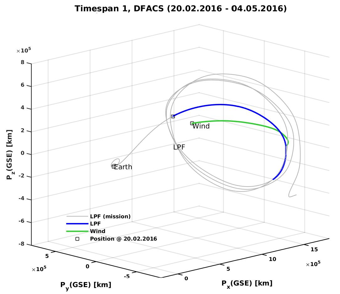
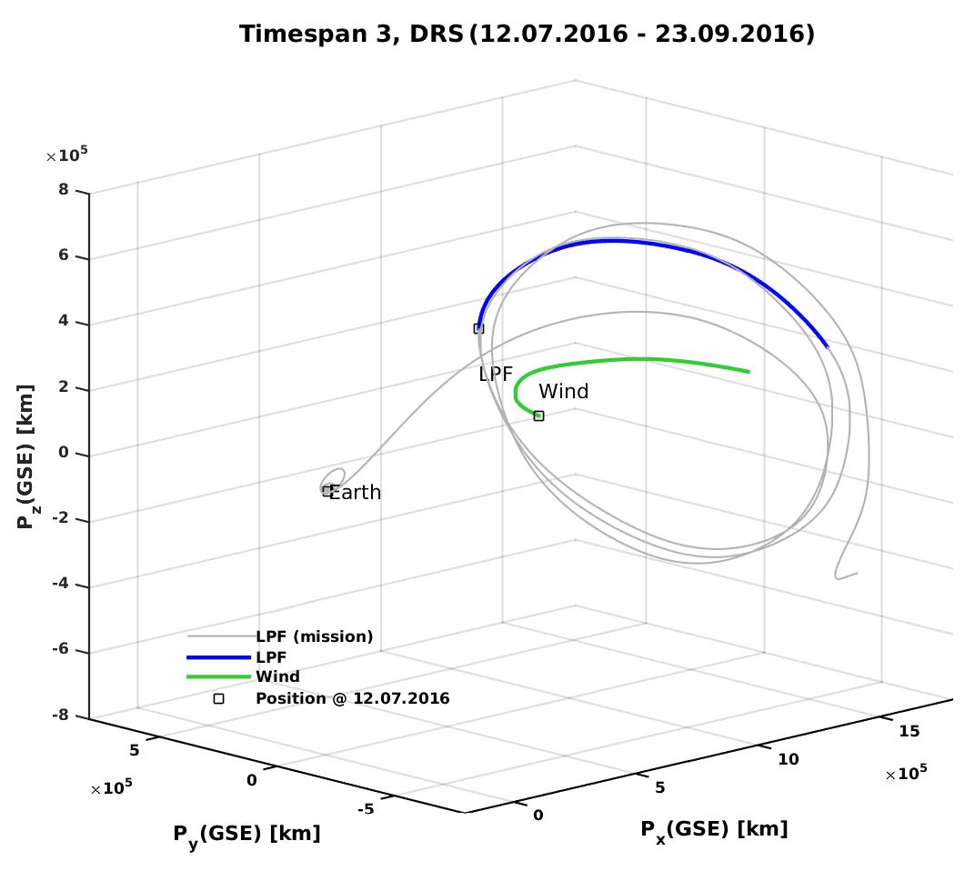
Figure 8: LPF and Wind orbits during the timespans indicated with TS1 and TS3.

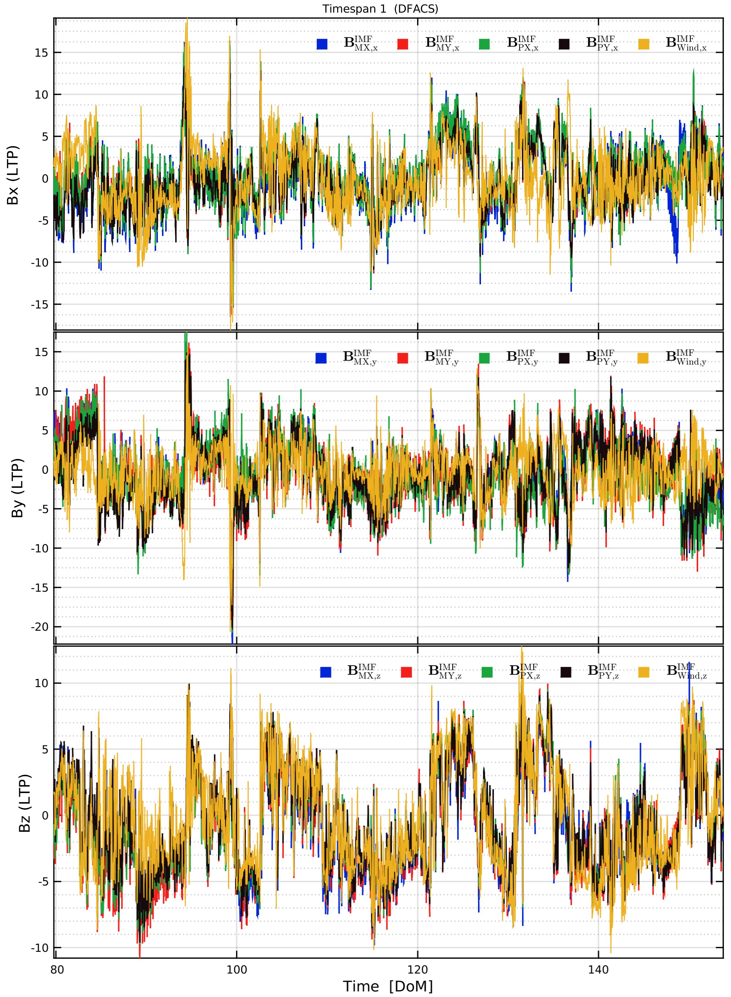
Figure 9: Estimated LPF IMF timeseries ($\mathbf{B}^{\mathrm{IMF}}_{\mathrm{MX}}$, $\mathbf{B}^{\mathrm{IMF}}_{\mathrm{MY}}$, $\mathbf{B}^{\mathrm{IMF}}_{\mathrm{PX}}$ and $\mathbf{B}^{\mathrm{IMF}}_{\mathrm{PY}}$) and Wind MFI measurements in the $\boldsymbol{\mathrm{R}}_{\mathrm{LTP}}$ reference frame for the TS1 time interval (see Table 2).

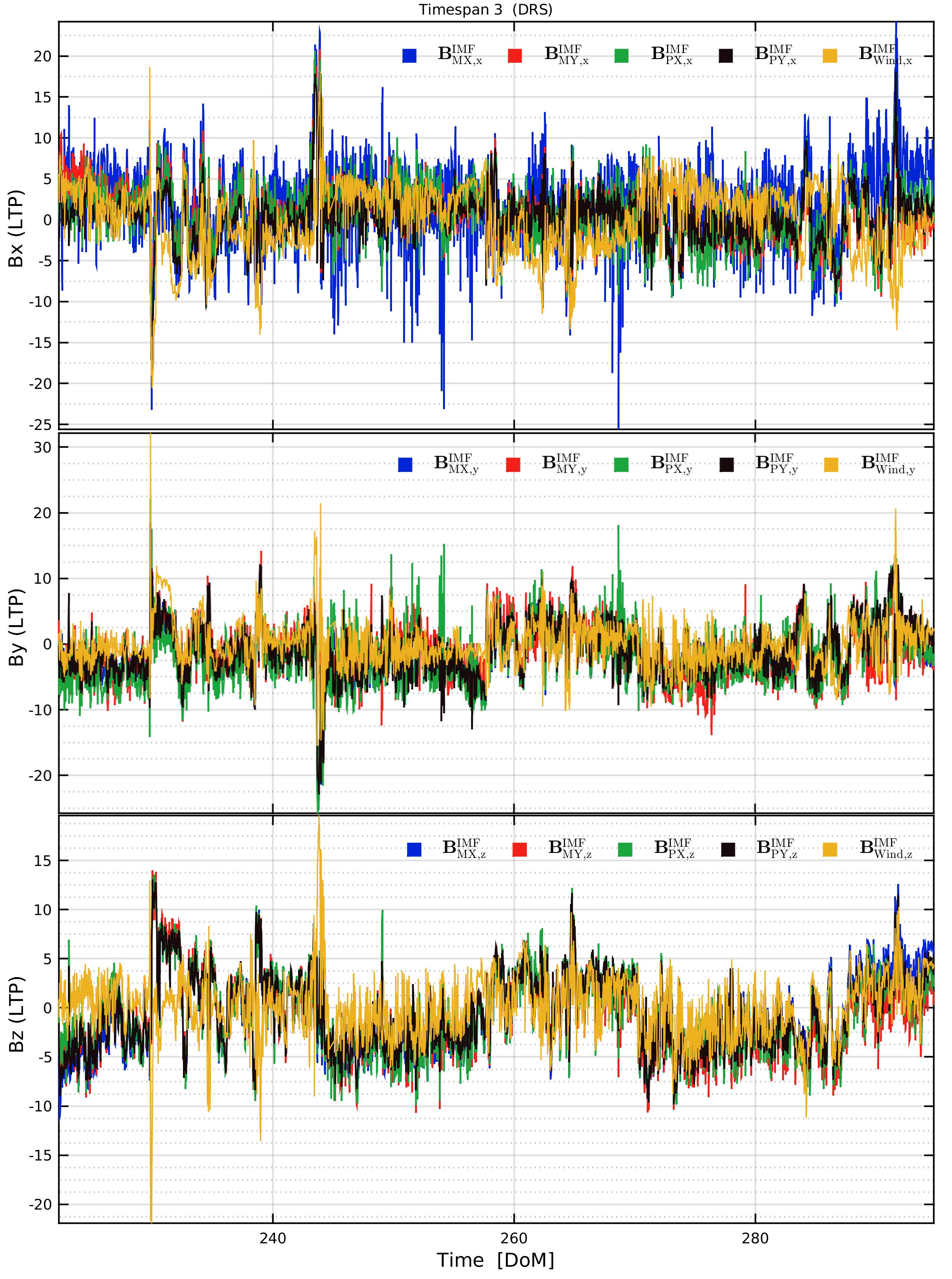
Figure 10: Same as Figure 9 for the TS3 time interval.

Figure 11: PSDs of the LPF magnetometer measurements ($\mathbf{B}^{\mathrm{MAG}}_{\mathrm{MX}}$, $\mathbf{B}^{\mathrm{MAG}}_{\mathrm{MY}}$, $\mathbf{B}^{\mathrm{MAG}}_{\mathrm{PX}}$, $\mathbf{B}^{\mathrm{MAG}}_{\mathrm{PY}}$) and of the estimated IMF. Datasets refer to TS1 (left panel) and to TS3 (right panel) time intervals (Tab. 2). The PSDs obtained by subtracting the Wind data from each LPF IMF measurement timeseries are also provided.

The empirical approach adopted in the present work to separate the IMF component from on-board platform magnetic field measurements has been applied to the entire LPF datasets. The IMF timeseries $\mathbf{B}^{\mathrm{IMF}}_{\mathrm{MX}}[t]$, $\mathbf{B}^{\mathrm{IMF}}_{\mathrm{MY}}[t]$, $\mathbf{B}^{\mathrm{IMF}}_{\mathrm{PX}}[t]$ and $\mathbf{B}^{\mathrm{IMF}}_{\mathrm{PY}}[t]$ obtained by processing the four magnetometer datasets are reported in Figure 12 in blue, red, green and black colors, respectively. In the same figure, the LPF IMF estimates are compared to contemporaneous measurements carried out with the MFI detector (in yellow) hosted on board the Wind S/C (NASA CDAWeb, https://directory.eoportal.org/web/eoportal/satellite-missions/). Data gaps are associated with magnetic experiments, electronics functional tests, faults and anomalies.

Figure 12: IMF measurement timeseries obtained with the four LPF magnetometers ($\mathbf{B}^{\mathrm{IMF}}_{\mathrm{MX}}$, $\mathbf{B}^{\mathrm{IMF}}_{\mathrm{MY}}$, $\mathbf{B}^{\mathrm{IMF}}_{\mathrm{PX}}$ and $\mathbf{B}^{\mathrm{IMF}}_{\mathrm{PY}}$ data appear in blue, red, green, and black, respectively). Simultaneous Wind magnetic measurements, $\mathbf{B}^{\mathrm{IMF}}_{\mathrm{Wind}}$, are also shown in yellow for comparison. Timespans TS13 and TS14 (Tab. 2) are ignored as discussed in Section 3 (hatched area). The $x$-axis indicates the mission lifetime in DOM.

A good agreement is found between Wind MFI and LPF IMF estimates during the whole mission duration.

In Figure 13 the time interval ranging from July 15 through August 4, 2016 is considered in particular.

Figure 13: Comparison between LPF and Wind IMF measurements in the $\boldsymbol{\mathrm{R}}_{\mathrm{GSE}}$ between July 15 and August 4, 2016.

In this figure, the IMF components inferred from the LPF on-board measurements are shown shown in the Global Solar Ecliptic reference frame ($\boldsymbol{\mathrm{R}}_{\mathrm{GSE}}$) in order to compare our results with the Wind IMF contemporaneous measurements. The LTP $z$-axis of the LPF magnetometer reference frame was aligned with the GSE $x$-axis during the mission lifetime, while the $\boldsymbol{\mathrm{R}}_{\mathrm{LTP}}$ $xy$-plane rotated around the LTP $z$-axis with a six month period. Between August 2 and August 3, 2016 the LPF S/C crossed a magnetic cloud. It is worthwhile to recall that a magnetic cloud is a coherent plasma structure characterized by a smooth rotation of the IMF and an enhanced magnetic field intensity with respect to the average value observed in the solar wind while temperature and plasma beta parameters (i.e. the ratio of the plasma pressure to the magnetic pressure) present lower values with respect to an undisturbed interplanetary medium (Burlaga et al., 1990). The LPF IMF data are compared to the magnetic field estimated by applying the Grad-Shafranov reconstruction technique based on the Wind S/C observations (Hu and Sonnerup, 2002; Hu, 2017; Benella et al., 2020). The comparison between the IMF components inferred from the GS reconstruction and the LPF observations is shown in Figure 14. The LPF IMF estimates are computed by averaging the data of the four magnetometers and are reported by considering a sampling time of one minute. Again, a good agreement is observed and this comparison allows for an independent validation of the results of our empirical approach within a few percent.

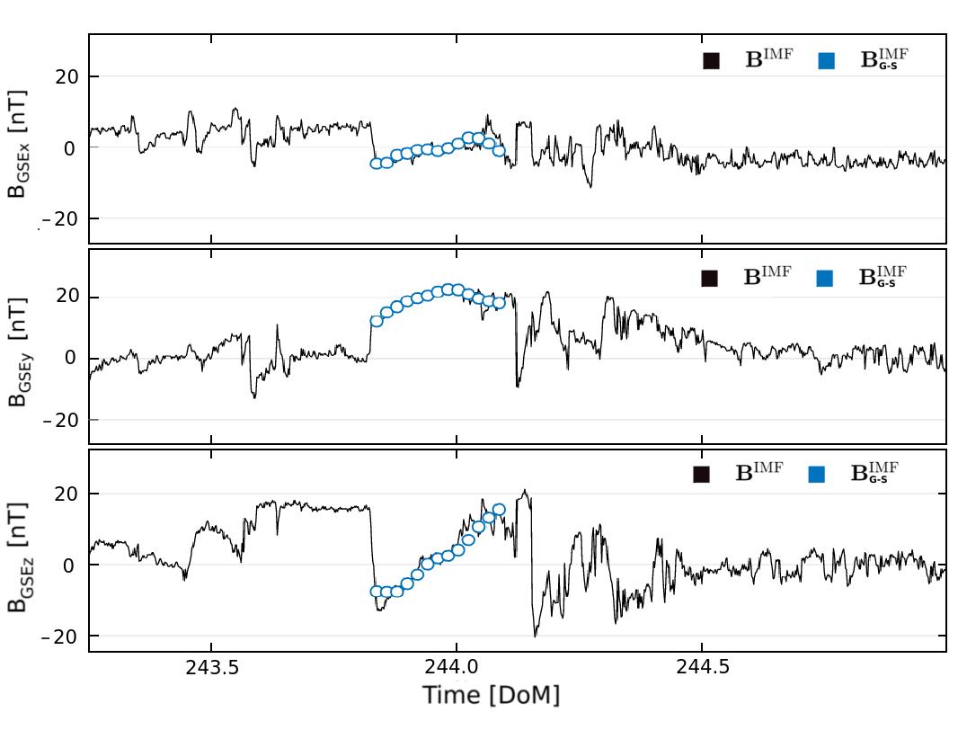
Figure 14: LPF IMF (black line) and IMF along the LPF orbit obtained with a Grad-Shafranov reconstruction based on Wind data of the magnetic cloud crossed by the S/C on August 2-3, 2016 (open blue circles). Each LPF IMF component was obtained by averaging the measurements of the four on-board magnetometers.

A similar work could be carried out for LISA that will also host platform magnetometers in order to monitor the transit of interplanetary magnetic structures. It is worthwhile to point out that contrarily to LPF, LISA will not benefit of other experiments gathering interplanetary magnetic field, plasma data and particle monitoring along its orbit.

6 Galactic and solar energetic particle events during the LISA mission operations

6.1 Galactic cosmic-ray energy spectrum during the solar cycle 26

The galactic cosmic-ray (GCR) flux in the inner heliosphere appears energy, time, space, and charge dependent. The overall GCR flux was observed to vary by a factor of four near Earth during the last three solar cycles when the majority of data to study the long-term variations of particles of galactic origin were gathered in space (Grimani et al., 2021a). Since LISA will orbit the Sun at 1 AU, both near-Earth GCR and SEP observations can be used to carry out long-term predictions of the overall particle flux during the mission operations by properly taking into account the solar activity expected during the solar cycle 26 (Singh and Bhargawa, 2019). The predicted sunspot number, the most widely used proxy of the solar activity during the solar cycle 26, is reported in Figure 15 and Table 7.

Figure 15: Sunspot number prediction for the solar cycle 26 (Singh and Bhargawa, 2019).

Year	SSN	SEP
2035	68	4.7
2036	76	5.3
2037	77	5.3
2038	74	5.1
2039	63	4.4
2040	42	2.9
2041	32	2.2
2042	21	1.5
2043	11	0.8
2044	1	0.07

Table 7: Expected sunspot number (SSN) and SEP events during the LISA mission with a fluence larger than the estimated GCR background.

The past solar cycle 24 has been the weakest of the last hundred years. According to Singh and Barghawa (Singh and Bhargawa, 2019), the next two solar cycles are expected to be even weaker. However, it is worthwhile to point out that the initial phase of the solar cycle 25 appears more intense than these predictions and other authors indicate an intensity similar to that of the solar cycle 23 (Diego et al., 2010; McIntosh et al., 2020; Diego and Laurenza, 2021). Quasi-eleven and quasi twenty-two year periodicities are observed in the GCR intensity associated with the solar activity and the GSMF polarity reversal, respectively. The force-field model by Gleeson and Axford (Gleeson and Axford, 1968) is adopted here for the prediction of GCR long-term modulation while the Nymmik model (Nymmik, 1999a, b) is considered to estimate the occurrence of SEP events with fluence larger than 10⁶ protons cm^-2 above 30 MeV during the LISA mission. The Gleeson and Axford model allows us to estimate the GCR flux in the inner heliosphere by assuming a time independent interstellar spectrum and a solar modulation parameter $\phi$ describing the effect of the solar activity modulation (see Armano et al., 2018a, where the details of our approach are illustrated). The sunspot number is correlated with the solar modulation parameter. After the LISA launch in 2035, the maximum expected number of sunspots is about 80 and, consequently, the solar modulation parameter may possibly vary between 600 MV/c and 700 MV/c, as in September 2015 for instance (see https://cosmicrays.oulu.fi/phi/Phi_mon.txt handled by the University of Oulu, Finland). This estimate appears consistent with the solar modulation values inferred from Maurin et al. (2020).

The proton energy spectrum above 70 MeV corresponding to the above solar modulation was obtained with the Gleeson and Axford model (bottom dot-dashed line in Fig. 16) parameterized according to Papini et al. (1996) and Armano et al. (2018a) as follows:

$$F(E)=18000\times(E+1.5)^{-3.66}\ E^{0.87}\ \ \ {\rm particles/(m^{2}\ sr\ s\ GeV),}$$ (10)

where E is the proton kinetic energy in GeV. The proton flux is considered in the figure since protons constitute 90% of the overall cosmic-ray bulk. We verified the reliability of this approach for the LISA Pathfinder mission in 2016-2017, by comparing our cosmic-ray proton flux predictions to observations carried out above 450 MeV n^-1 by the AMS-02 experiment during the same period on the Space Station (see Aguilar et al., 2018). Our predicted GCR integral proton flux at the LPF launch in December 2015 was found only 10% higher than the AMS-02 data (Grimani et al., 2019).

6.2 Estimates of solar energetic particle event occurrence during the LISA mission

Nymmik (Nymmik, 1999a, b) has found that the SEP fluence distribution follows a power-law trend with an exponential cutoff for increasing values of the fluence. This model applies to proton fluences ranging between 10⁶ and 10¹¹ protons cm^-2 above 30 MeV, where 10⁶ protons cm^-2 represents the fluence that approximately corresponds to the background of GCRs near solar minimum. The Nymmik model was developed on the basis of SEP event measurements carried out with the IMP-7 and IMP-8 S/C during the solar cycles 20-22 and from proton fluxes estimated with radionuclide observations in lunar rocks generated in the last few million years. The method is illustrated in the following (Storini et al., 2008). The yearly number of SEP events, $<n>$ is assessed on the basis of sunspot number predictions, $<N>$:

$$<n>=0.0694<N>.$$ (11)

In order to estimate the number of events per interval of fluence, $f$, a normalization constant C must be then set by integrating the equation:

$$dn=Cf^{-1.41}e^{-f/f_{c}}df,$$ (12)

and by equaling it to $<n>$. In the above equation $f_{c}$ is assumed equal to 4$\times$10⁹. It is pointed out that 65% of the events are expected to belong in the fluence range 10⁶-10⁷ protons cm^-2.

In Grimani et al. (2012) the expected number of SEP events satisfying the Nymmik model was compared to observations carried out between 1986 and 2004. Model and data were found in agreement within a factor of two. The expected number of SEP events during the time the LISA mission will remain in space, possibly between 2035 and 2044, is reported in Table 7.

As a worst case scenario, the occurrence of a SEP event with 10⁹ protons cm^-2 fluence in the next years should be also considered to estimate the LISA TM charging. The typical rate of occurrence of these events is one every sixty years. The last one, characterized by particle acceleration above 100 MeV n^-1, was observed on February 23, 1956 (Vashenyuk et al., 2008). The proton fluxes observed during the evolution of SEP events of different intensities are shown in Figure 16 in comparison to the minimum expected galactic flux over the LISA mission duration.

7 Next Generation Radiation Monitor

The ESA NGRM is small ($<$1 dm³), light ($<$ 1 kg) and characterized by a low power consumption ($<$ 1 W). This detector is optimized for low-energy particle measurements in harsh radiation environments, typical of SEP events and of particles magnetically trapped in the Earth and other planetary magnetospheres. The NGRM consists of two units. The proton unit allows for the measurement of the proton flux between 2 MeV and 200 MeV. In Figure 16 proton energy spectra of particles of galactic and solar origin are compared. Protons with energies smaller than 200 MeV constitute a minor percentage of particles of galactic origin (continuous lines) at both solar minimum (upper curve) and maximum (lower curve). As it was shown in the previous section, the bottom dot-dashed curve represents the minimum flux of galactic protons expected during the LISA mission. In the same figure the proton energy spectra observed during the evolution of SEP events of different intensities appear softer than the GCR energy spectrum and, consequently, the particle flux below 200 MeV is representative of the total solar proton flux. As a result, the NGRM is an optimum monitor of the solar particle flux. Linear energy transfer of ions can be also measured with this detector. The electron unit is meant to monitor electrons in the energy range 100 keV-7 MeV.

In Figure 17 solar (top dashed and dotted curves) and galactic (solid, dot-dashed and bottom dashed lines) electron fluxes are compared (Grimani et al., 2009a, b). A sudden increase of the electron flux at MeV energies is a precursor of a solar energetic proton event due to particle velocity dispersion. Solar electron fluxes showing two different spectral indices indicate impulsive SEP events associated with proton acceleration below 50 MeV. Conversely, a single spectral index characterizes the solar electron flux associated with gradual events with proton acceleration above 50 MeV. In Grimani et al. (2009a) and references therein it was shown that the intensity of the solar electron flux in the MeV range is similar to the proton flux intensity in the 50 MeV range. The NGRM has excellent SEP event short-term forecasting and measurement capabilities. LISA will allow us to carry out the first multispacecraft SEP event observations at a few million kilometers with twin detectors. The LISA data will be also compared to observations gathered near Earth at 50 million kilometers. Conversely, the GCR flux short-term variations will not be nicely monitored with NGRM.

The geometrical factor of the NGRM for GCR measurements is of about 0.01 cm², approximately hundred times smaller than that of the detector hosted on board LPF. As a matter of fact, the NGRM will not allow us to monitor the dynamics of non-recurrent GCR short-term variations of typical durations of three-four days and grossly only recurrent GCR short-term variations that were found to last an average of 9 days with LPF (Grimani et al., 2020).

Figure 16: Minimum and maximum proton energy spectra of galactic origin observed near Earth (top and bottom continuous lines, respectively). The bottom dot-dashed line represents the minimum proton flux expected during the LISA mission. Dashed lines (December 14, 2006; Adriani et al. (2011)), dotted lines (May 7, 1978; McGuire and von Rosenvinge, 1984) and top dot-dashed lines (February 23, 1956; Vashenyuk et al., 2008) represent solar proton fluxes observed during the evolution of SEP events of different intensities. The vertical black line indicates the maximum energy of the NGRM proton spectrum measurement capability.

The classification of interplanetary processes associated with GCR short-term variations observed with LPF are reported in Armano et al. (2018a, 2019a). The evolution of each GCR short-term depression is unique and depends on the energy differential flux of GCR particles at the transit of subsequent interplanetary structures. Consequently, the average monthly GCR flux observations are not representative of the GCR flux at shorter timescales. Moreover, it is of fundamental importance to maintain separated the effects of cosmic-ray long-term modulations from short-term variations, due to a different dependence on the particle energies for the estimate of the LISA and LPF TM charging. Only low statistical uncertainty data gathered hourly in space above a few tens of MeV n^-1 would allow us to disentangle the role of long-term and short-term solar modulation of the GCR flux in the LISA sensitivity band.

The evolution of individual recurrent and transient GCR variations studied with data gathered on board the LPF S/C were compared to contemporaneous Earth neutron monitor observations. This comparison revealed that very poor clues can be obtained on the physics of GCR flux short-term variations in space from ground data affected by low-energy particle flux attenuation in the atmosphere and by the geomagnetic cut-off. For instance, recurrent GCR flux depressions of intensities $<$ 5% detected on board LPF were not observed on neutron monitors by revealing that only particles with energies smaller than neutron monitor effective energies ($>$ 10 GeV; see for details Armano et al., 2019a) were involved in these processes. It is worthwhile to recall that particle count rates observed with neutron monitors vary proportionally to the cosmic-ray flux at energies larger than the effective energy (Gil et al., 2017), thus providing a direct measurement of the GCR flux at the top of the atmosphere above 10 GeV. While GCR recurrent short-term variations observed in space were associated with particle modulation below a few GeV within 1% uncertainty, Forbush decreases (sudden drops of the GCR flux observed at the transit of ICMEs, Forbush, 1937; 1954; 1958) were characterized by a GCR particle flux modulation at energies above 10 GeV. Three Forbush decreases were observed with LPF and neutron monitors on July 20 and August 2, 2016 and on May 27, 2017. The event depression amplitudes were found of 5.5%, 9% and 7% in space and of less than 2-3% in neutron monitor observations (Armano et al., 2019a). In conclusion, also neutron monitor observations will not allow us to properly monitor the LISA TM charging during galactic cosmic-ray flux short-term variations. This may be useful, for instance, if TM glitches of unknown origin will be observed. As a result, a dedicated cosmic-ray detector with characteristics similar to those of the LPF PD would be more than recommended for LISA to improve the monitoring of the transit of interplanetary magnetic structures and high-speed streams.

Figure 17: Solar electron fluxes associated with impulsive (upper dashed line) and gradual (dotted line) SEP events (Grimani et al., 2009a). The continuous line, the dot-dashed line and the bottom dashed line represent minimum and maximum interplanetary and galactic electron fluxes observed during a negative polarity period (A$<$0) of the GSMF (when the solar magnetic field lines enter the North pole of the Sun) during which the flux of negative particles is maximum with respect to periods of positive GSMF polarity and similar conditions of solar activity (Grimani et al., 2009a). The vertical continuous line indicates the maximum electron energy measured by the NGRM. It can be observed that below 7 MeV the solar electron flux overcomes by several orders of magnitude the interplanetary and galactic components allowing for SEP event forecasting.

8 Conclusions

Spurious forces acting on the TMs of the future LISA and LISA-like interferometers for gravitational wave detection in space will be monitored and mitigated in order to improve the mission performance. Magnetometers and particle detectors will be hosted on board the LISA S/C to monitor the variations of the magnetic field and the TM charging process. Precious clues were obtained about the interplanetary medium impact in limiting the LISA performance with the LPF mission flown in 2016-2017 around the L1 Lagrange point to test the LISA technology. The LPF magnetometers measured a magnetic field varying from $700$ to $1200\,\mathrm{nT}$ near the TMs while the IMF values in L1 ranged between $1$ and $25\,\mathrm{nT}$. The on-board generated magnetic field components were observed to vary by about $150\,\mathrm{nT}$ on timescales of months and of $20-30\,\mathrm{nT}$ daily. An empirical approach was considered in the present work to disentangle the IMF from the on-board originated magnetic field by processing the LPF platform magnetometer measurements. An agreement within a few percent was found between the LPF estimated IMF components and those provided by the dedicated MFI instrument on board the Wind S/C also orbiting around L1. A similar approach could be considered for the future gravitational wave experiments carried out in space. Provided the availability of the whole housekeeping dataset, an empirical magnetic field noise model can be produced when a S/C is already in-flight, even in the case that platform magnetometers are immersed in a strong varying and direction dependent on-board generated magnetic field. Solar energetic particle event short-term forecasting and evolution monitoring will be also carried out with the NGRM on board the LISA S/C. An additional particle detector dedicated to galactic cosmic-ray variation observations should be also included in the set of detectors meant for the mission diagnostics. LISA and the second generation LISA-like interferometers will also naturally play the role of multipoint observatories for SEP events and interplanetary large-scale structure monitoring with magnetometers used in combination with dedicated GCR detectors.