The diagnostics subsystem on board LISA PathFinder and LISA

Abstract

The Data and Diagnostics Subsystem of the LTP hardware and software are at present essentially ready for delivery. In this presentation we intend to describe the scientific and technical aspects of this subsystem, which includes thermal diagnostics, magnetic diagnostics and a Radiation Monitor, as well as the prospects for their integration within the rest of the LTP. We will also sketch a few lines of progress recently open towards the more demanding diagnostics requirements which will be needed for LISA.

Keywords: LISA, LISA Pathfinder, gravity wave detector, interferometry, diagnostics.

1 Introduction

LISA is a technologically sophisticated mission. In its current baseline design, an arm length of 5 million kilometers is envisaged, and its acceleration noise is required to satisfy [1]

$$S_{\delta a,{\rm LISA}}^{1/2}(\omega)\leq 3\times 10^{-15}\,\left\{\left[1+\left(\frac{\omega/2\pi}{8\ {\rm mHz}}\right)^{\!\!4}\right]\!\left[1+\left(\frac{0.1\ {\rm mHz}}{\omega/2\pi}\right)\right]\right\}^{\!\frac{1}{2}}\ {\rm m}{\rm s}^{-2}/\sqrt{\rm Hz}$$ (1)

in the frequency band between 0.1 mHz and 0.1 Hz.

LISA PathFinder (LPF) has a reduced acceleration noise budget, both in magnitude and in frequency band [2],

$$S_{\delta a,{\rm LPF}}^{1/2}(\omega)\leq 3\!\times\!10^{-14}\,\left[1+\left(\frac{\omega/2\pi}{3\ {\rm mHz}}\right)^{\!\!2}\right]\,{\rm m}{\rm s}^{-2}/\sqrt{\rm Hz}$$ (2)

in the frequency band between 1 mHz and 30 mHz. This noise is the result of various disturbances which limit the performance of the instrumentation on-board. A number of these can be specifically monitored and dealt with by means of suitable devices, which form the so called Diagnostics Subsystem. In the case of LPF, these include thermal and magnetic diagnostics, plus the Radiation Monitor (RM), which provides counting and spectral information on ionising particles hitting the proof masses. The purpose of this note is to summarise the latest developments on the LPF Diagnostics Subsystem, developed in Barcelona, including some preliminary research results on the extension of their performance in view of the future LISA. The diagnostics in LPF, as a technology precursor of LISA, are intended to help design a quieter environment in the LISA spacecraft. Their role in LISA is still to be defined, but they will likely work as a noise debugging tool, much in the same spirit as in LPF, which will provide house-keeping data and assist in GW signal dig-out.

Background to the diagnostics motivation and main requirements will be omitted here, but the reader will find details in [3] and references therein. In this paper we will sequentially review the latest relevant results on each of the diagnostics items.

2 Thermal diagnostics

The temperature stability required to prevail inside the LCA (LTP Core Assembly, LTP = LISA Technology Package) is, in spectral density of temperature fluctuations, 10^-4 K Hz^-1/2 in the measuring bandwidth. Studies carried through at IEEC during the prototyping stage determined that the only option compatible with reliable temperature measurements at that level was the use of thermistor devices —or NTC, Negative Temperature Coefficient devices [4]. After successful verification that the NTCs plus their front-end electronics worked OK, the circuitry was integrated in the DMU (Data Management Unit, the LTP computer), and flight hardware and software were recently submitted to further test. The results are shown in Figure 1.

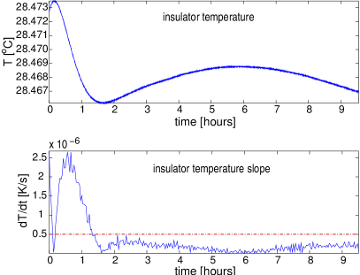
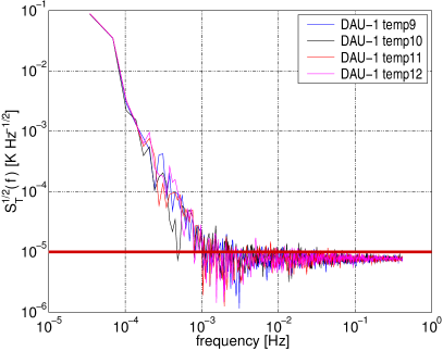
Figure 1: Flight model temperature sensor behaviour. Left panel: 9.5 hour data run, as read by the NTCs. The upper graph shows the raw data, and the lower graph its time variations. Note the slope is below the critical value of 0.5 $\mu$K/sec only when the testbed has reached thermal stability after almost two hours. Right panel: spectral density of noise for 4 NTCs: all of them are below the required 10^-5 K Hz^-1/2 threshold throughout the measuring bandwidth. Data to produce the plot correspond to the period of low temperature slope.

During the data taking run, the sensors were placed inside an insulator jig which strongly damps any ambient temperature fluctuations. The jig consists in an aluminium metal core, where the NTCs are attached, surrounded by a thick layer of polyurethane, with a very low thermal conductivity coefficient [5]. The damping efficiency of the device is large enough for thermal screening of its interior, but the connecting harness between the sensors and the electronics outside constitutes a leakage line which does degrade in practice the conditions for the test. In order to maintain the temperature of the NTCs stable over long periods of time, a temperature feedback control was added to the system —see next paragraph. Another factor of improvement was to keep ambient temperature as stable as feasible. For this, the experiment was done inside a well insulated anechoic chamber in the Institute’s building basement floor. To ensure temperature stability conditions, the whole setup (insulating jig, front-end electronics and computers) was locked and left untouched for two days before starting the experiment.

The DMU has two identical redundant DAUs (Data Acquisition Units), and the plots in 1 reflect the data taken by DAU-1. A very important circumstance has to be taken into consideration when the data analysis is performed. This is the temperature drifts, which need to be maintained small, more specifically, $|dT/dt|<$0.3 $\mu$K/sec. The reason is the non-linear behaviour of the ADC (Analog-to-Digital Converter), which introduces spurious noise at low frequencies due to quantisation errors. The ADC has 16 bits, and the effect could be avoided with a larger bit depth ADC —which is not available for flight. The temperature feedback control system in the jig’s aluminium core mentioned above takes care of the stability conditions of the NTCs temperature at very low frequencies [6], thereby enlarging the length of measuring time available for analysis. Usable data in the reported run were 8 hours (see left panel, lower plot), not a very long stretch yet widely sufficient to obtain a reliable spectral estimation down to 1 mHz.

The spectra shown in the right panel correspond to four sensors (labelled 9 through 12), attached to one of the three multiplexer boards in the DAU. In order to detect temperature fluctuations in the LCA below the stability conditions of 10^-4 K Hz^-1/2, a requirement was set on the temperature sensing of 10^-5 K Hz^-1/2 [7]. As can be seen, all these sensors perform according to the requirement in the entire LTP band, from 1 mHz to 30 mHz.

2.1 Looking into LISA

Noise steeply rises towards lower frequencies, which in turn poses the question of how difficult it may be to reach the lower frequency band of LISA with suitable sensitivity at 0.1 mHz. Recent research work at IEEC has shown that neither the current electronics design nor the sensors themselves are limiting factors. Rather, it is the experimental conditions, described above, which appear to be unsuitable to properly assess the real performance capabilities of the thermal sensing system: heat leakage through the wiring and insufficient screening capacities of the surrounding jig have proved to be at the root of the problem, instead. Preliminary experiments with an improved wiring concept, and use of differential temperature measurements has shown that it is already possible to reach a level of noise below 10^-5 K Hz^-1/2 at 0.1 mHz with no changes to the electronics and with the same NTCs. It is conjectured that even 1 $\mu$K Hz^-1/2 can be attainable. Although LISA requirements are still not fully defined in this area, these results are really promising. The reader is referred to Sanjuán’s contribution to this volume for further details and plots on this important matter.

2.2 Heaters

The availability of excellent thermometers is not very useful of itself. Actually, their use is to convert temperature fluctuation information into test mass acceleration noise. In other words, we would like to know which fraction of the total LTP readout noise is due to temperature fluctuations. For this, calibration is needed, which will translates temperature measurements to acceleration readout. In the LTP, the procedure to obtain such relationship is the use of controlled, high signal-to-noise ratio thermal signals applied in suitably chosen locations, and measure the observed system response in parallel with temperature measurements. A (matrix) transfer function is thus obtained, which can subsequently be applied to the thermometers’ readings to determine the specific weight of temperature noise in the LTP total noise [3].

Several modelling and laboratory experiments have been done to characterise the above procedure, with very interesting results [8, 9]. In flight, the analysis is more complicated, as the calibration process interacts with the full LTP dynamics loop. The on-ground experiment analysis results can be directly fed into that loop, and the mission master plan naturally includes suitable protocols to deal with the heater signals and the inference of the corresponding transfer functions. The reader is referred to Nofrarias’s contribution to the JPCS volume of this Proceedings for the latest progress on this matter.

3 Magnetic diagnostics

Again, this section only reports on the latest results on LTP magnetic diagnostics. The reader will find background information in [3]. The LTP Test Masses (TMs) are two cubes 4.6 cm to the side, weighing 1.96 kg each. They are made of an alloy of gold and platinum with 70 % Au + 30 % Pt. To cast such an alloy is a process where ferromagnetic impurities can contaminate the alloy structure, thus leaving a remanent magnetic moment ${\bf m}_{0}$ in the TM. Likewise, magnetic susceptibility, $\chi$, will be present. These are required to comply with the following constraints [2]:

$$|\chi|<10^{-5}\ ,\quad|{\bf m}_{0}|<10^{-8}\ {\rm Am}^{2}$$ (3)

In spite of these low values, magnetic field and gradient fluctuations in the TMs result in spurious forces on them, causing acceleration noise which adds undiscriminated to the LTP readout. In order to diagnose the state of the magnetic environment, a set of high sensitivity vector magnetometers are placed in the LCA wall —see figure 2.

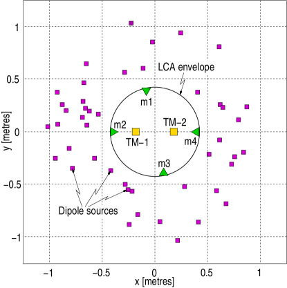
Figure 2: Projection view of the dipole magnetic sources in the LPF spacecraft (small squares), the TMs (larger squares) and the magnetometers (triangles).

These magnetometers are tri-axial fluxgate magnetometers which have a relatively large Permalloy core. They are very sensitive —see below—, but should be kept somewhat far from the TMs to avoid magnetic back action disturbances on the latter.

Figure 2 also displays the positions of identified sources of magnetic field in the LCA [10]. These sources are all beyond the LCA walls, and come from various circuitry and other magnetic components in the spacecraft. Clearly, the magnetic field in the TMs is smaller than it is in the magnetometers, since it decays towards the inner region of the LCA as it is produced by magnetic dipoles. This poses a problem of interpolation between the magnetometers’ readouts to obtain the actual field in the TMs positions. We now describe how to address this problem, according to our current understanding.

3.1 Magnetic field interpolation

We assume the TMs are small size compared to the LCA volume, hence we consider the magnetic field, ${\bf B}({\bf x})$ inside the LCA to be mostly a vacuum field. This means $\nabla$$\times$${\bf B}$ = $\mbox{\boldmath$\nabla\cdot$}{\bf B}$ = 0, or

$${\bf B}({\bf x})=-\mbox{\boldmath$\nabla$}\Psi({\bf x})\ ,\quad\nabla^{2}\Psi({\bf x})=0$$ (4)

where $\Psi({\bf x})$ is a scalar function. If this is expanded in terms of spherical harmonics, $Y_{lm}$, then ${\bf B}({\bf x})$ ensues as

$${\bf B}({\bf x})=\frac{\mu_{0}}{4\pi}\,\sum_{l=1}^{\infty}\,\sum_{m=-l}^{l}\,M_{lm}\,\mbox{\boldmath$\nabla$}\left[r^{l}Y_{lm}({\bf n})\right]\ ,\quad r\equiv|{\bf x}|\ ,\quad{\bf n}\equiv{\bf x}/r$$ (5)

where $M_{lm}$ are the multipole coefficients of the expansion. Ideally, an infinite number of coefficients are necessary to calculate ${\bf B}({\bf x})$, which would be possible if the field was known in all points of a closed surface not containing any field source. In real practice, we only have four magnetometers, so the number of multipole coefficients we can actually determine is fixed by this circumstance. The counting is easy to do: there are 12 sensor data channels, three per magnetometer (recall they are tri-axial). The number of $M_{lm}$ we can calculate is accordingly 12, or less. There is no monopole contribution to B, of course, there are three dipole coefficients, five quadrupole, seven octupole, etc. The series expansion in equation (5) must thus be cut at $l$ = 2, since continuing it up to $l$ = 3 would require 3 $+$ 5 $+$ 7 = 15 $M_{lm}$, but we can only estimate 12. The following is thus our best approximation:

$${\bf B}_{\rm approx}({\bf x})=\frac{\mu_{0}}{4\pi}\,\sum_{l=1}^{2}\,\sum_{m=-l}^{l}\,M_{lm}\,\mbox{\boldmath$\nabla$}\left[r^{l}Y_{lm}({\bf n})\right]$$ (6)

Next task is to determine the 8 dipole $+$ quadrupole coefficients. This we do by a least square method, where we define the square error as

$$\varepsilon^{2}(M_{lm})=\frac{1}{2}\,\sum_{s=1}^{4}\,\left|{\bf B}_{\rm approx}({\bf x}_{s})-{\bf B}_{\rm measured}({\bf x}_{s})\right|^{2}$$ (7)

where $s\/$ is an index labelling the magnetometers, located at positions ${\bf x}_{s}$, and ${\bf B}_{\rm measured}({\bf x}_{s})$ is the (vector) readout of the $s\/$-th magnetometer. By solving the system of equations $\partial\varepsilon^{2}/\partial M_{lm}$ = 0 we find $M_{lm}$ for $l\/$ = 1,2, $m\/$ = $-l,\ldots,l$. Feeding them into equation (6) with x = ${\bf x}_{\rm TM}$, the positions of the test masses, we get the desired interpolation to estimate the field values at the TMs.

In order to verify the efficiency of this analysis, the following procedure was implemented: series of magnetic moments of the dipole sources were simulated randomly —with some constraints on their moduli, as indicated by the estimates at Astrium-Stevenage [10]—, and the field reconstruction algorithm was subsequently applied to each series. Then the values of the so reconstructed field at the TMs were compared with the exact ones, also case by case. Unfortunately, the results appear to be poor: deviations between obtained and expected figures vary between quite good (less than 10%) and rather disappointing (factors of 5 and eventually more). The reason for this poor result is easy to discover: the series (6) only provides a linear interpolation algorithm between field values at the LCA boundary, where the sensors are, to its interior, which cannot accurately account for the fact that the field components have a trough somewhere there —its position and depth depending on the particular dipole distribution outside.

3.2 New magnetic diagnostics concepts for LISA

The magnetometers are required to have a level of noise below 10 nT Hz^-1/2 in the LTP bandwidth. The fluxgates to be flown on-board LPF are comfortably compliant with that, as shown in figure 3, left panel.

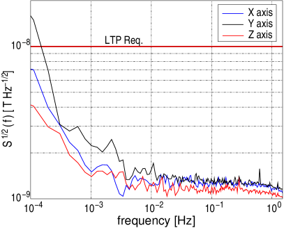
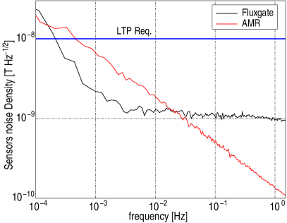
Figure 3: Left panel: spectral density of noise of each of the three channels of an LTP fluxgate magnetometer. Right panel: comparison of the performance of the latter with that an AMR magnetometer.

Such excellent performance, however, does not quite match the quality of the results we can derive from their output, as discussed in the previous section. A more faithful reconstruction of the magnetic field at the TM positions requires the magnetometers to be closer to them, but fluxgates cannot be mounted there: back-action would be unacceptably high, and space resolution is poor (the sensor heads are $\sim$2 cm long). An investigation of alternative solutions has just begun at IEEC to improve magnetic diagnostics for LISA, whereby AMR (Anisotropic Magneto-Resistance) devices are being considered. These are very tiny, and at least three or more per TM could be attached to the spacecraft structure appreciably closer to the TMs without risk of back action effects. Preliminary results on the performance of AMRs is shown in figure 3, right panel, which do look encouraging. Details on this matter will be found in Mateos’s contribution to the JPCS volume of this Proceedings, where various aspects of the problem are addressed, including magnetic properties of the AMRs.

3.3 Control coils

Like with thermometers, magnetic field measurements are of themselves of little use. We need to convert magnetic field and gradient fluctuations into LTP acceleration noise. For this, controlled magnetic forces are applied to the TMs by means of non-homogeneous fields generated by coils, which will serve calibration purposes of the magnetometers’ readouts —see background information details in [3]. Because of the magnetic susceptibility of the TMs, magnetic forces on them depend on coupling of the magnetic field to its gradient. Acceleration fluctuations accordingly depend on magnetic field gradient fluctuations as well as on field DC values. This in turn dictates that DC fields generated by the coils should be very stable not to degrade their performance. Tests to check the current stability requirements in the coils are underway at the time of writing. Provisional results look so far satisfactory. Test Reports will be formally written after full analysis of the data is complete.

4 The Radiation Monitor

LPF will be stationed in a Lissajous orbit around Lagrange point L1, some 1.5 million km away from the Earth in direction to the Sun. There, the spacecraft will be exposed to various ionising radiations coming from the Galaxy and from the Sun. Some of these charged particles, will be stopped by the spacecraft structure surrounding the TMs, while others will make it to the TMs. The latter are particles having energies above a threshold of about 100 MeV/nucleon, as shown by detailed simulations done at Imperial College [11]. The excess charge deposited in the TMs depends on the primary energy of the incoming particle, since secondary particles are generated inside the TMs as the primary travels across the TM volume. The charge deposit is of course a random process which results in acceleration noise due to interactions with the electric system which monitors the position of the TMs in their enclosure, to fluctuations of the position of the TMs relative to the electrostatic centre of the electrode housing, and to Lorentz interaction with the environmental and interplanetary magnetic field [12].

The LTP is equipped with a system of ultraviolet lamps which are needed to purge (by photo-electric effect) the charge accumulated in the TMs. By accurately matching the discharge rates to the charging rates the noise due to charging can be minimised. However, the GRS (Gravitational Reference Sensor) can only track charging rates by averaging over certain periods of time. The Radiation Monitor (RM) is capable of measuring these charging rates over significantly shorter periods —see below—, thereby producing data which will be used to help match the measured charging rates to the discharging rates, or else to clean LTP data by off-line analysis [13]. Further details on this will be found in Diana Shaul’s contribution to this Proceedings.

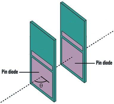
Figure 4: Left panel: RM concept: two PIN-diodes in telescopic configuration can both count single particles and measure their energy when events are detected in coincidence. Right panel: actual hardware schematics. The horizontal plates inside the box indicate the two PCBs, each connected to one of the PINs.

The RM design was based on detailed simulations of the LPF spacecraft and the LTP structure [11], and with a philosophy of making it simple and light while, at the same time, being able to provide not only particle counting but also spectral estimation to distinguish Galactic Cosmic Rays (CGR) from Solar Energetic Particles (SEP). The concept to implement such measurements is shown in figure 4, left. Two silicon PIN diodes are placed parallel to each other in a telescopic configuration. Each diode can count single particle events, but cannot tell whether the particles were charged or not. Events detected in coincidence in both PINs do instead correspond to charged particles, and their primary energy is inferred form the energy deposition. There is however some uncertainty here, due to degeneracy associated with the RM acceptance angle: higher energy particles with oblique incidence may deposit the same energy as lower energy particles which impact perpendicular to the PINs [14].

4.1 Technical details of the RM

The RM delivers data accumulated over periods of 614.4 seconds ($\sim$ 10 minutes), and sends them to the DMU in the form of histogrammes [15]. Figure 5 displays the structure of one of such histogrammes, with maximum bit depth in each bin, according to the maximum foreseen event rates, both in single events and coincidences, as well as in energy depositions. The latter range from 0 (actually $\sim$ 20 keV, due to noise) for the fastest incoming particles to 5 MeV for the slowest ones. Binning this range in 1024 equal length intervals provides an energy resolution of nearly 5 keV.

Figure 5: RM data histogramme: the first 1024 bins contain deposited energy of coincident events, while the remaining 60 bins contain number of singles counts, registered every 10.24 seconds. It takes 614.4 seconds to build up a complete histogramme. Total bit rate is 17.8 bits/sec.

The RM ADC has 16 bits, and sampling rate is 100 Hz. Data are accumulated in memory until they are sent to the DMU after 60 passages. In the first passage, singles are counted and stored in the first singles bin, in the second passage, singles are counted and stored in the second singles bin, and so on. In each passage, the energy deposited by events detected in coincidence in both PIN diodes is determined, the 1024 energy deposition bins scanned, and the number of events stored in the corresponding energy bins. Each passage therefore takes 10.24 seconds, hence 614.4 seconds are needed to fill up the 60 passage histogramme.

The estimated average of RM GCR singles counts is 4 c/s, and 0.4 c/s for coincident events. The largest SEP events observed so far can generate up to a few thousand singles c/s, and about 10 times less in coincidence. Therefore the RM electronics should be able to cope with such large events without degrading its performance. A conventional 5000 c/s was thus set as the requirement, which is comfortably satisfied by the RM: indeed, each singles bin can accept up to 2¹⁶ = 65,536 events in 10.24 seconds, i.e., 6400 c/s. The depth of the energy bins seen in figure 5 is uneven, based on the fact that large energy depositions are less frequent than small ones. This was done to reduce RM telemetry usage, but towards the end of May-2008 the LPF Science Working Team adopted a simplified scheme whereby all energy bins have maximum depth, i.e., 16 bits, which does not entail any significant increase in the mission telemetry budget.

The RM prototype underwent tests at the Proton Irradiation Facility of the Paul Scherrer Institute (PSI) in late 2005 which proved fully successful [16]. Since then, the initial IFAE design was used by NTE, the Spanish industrial contractor, to manufacture a RM EQM, with a number of modifications to make it handy for integration and flight. The EQM RM was recently debugged and green light for production of the FM (Flight Model) was given. The FM is expected to be finished by the end of 2008, and it will be submitted to further tests at PSI to verify basic functionality issues. The test will be milder than that done with the prototype, as strong irradiation may damage the device.

5 Conclusion

The diagnostics subsystem of the LTP will provide very useful noise debugging information, which will help us understand the nature of that noise, thence eventually guiding in various ways the progress towards the improved sensitivity needed for LISA.

The LTP diagnostics subsysten must comply with a number of requirements on sensitivity and performance, which have been implemented and tested to satisfaction at IEEC. Temperature measurements have been made in rather demanding conditions of environmental thermal stability —actually, significantly better than those in the LCA during flight— which ensure performance is cleanly assessed. The latest results reported in section 2 show that FM parts comply with the requirement of 10^-5 K/$\sqrt{\rm Hz}$ throughout the measuring bandwidth. Beyond these results, further investigation of system response at frequencies below 1 mHz has shown that both LTP sensors and front-end electronics maintain a level of noise of 10^-5 K/$\sqrt{\rm Hz}$ down to LISA’s lower end at 0.1 mHz. This is an extremely encouraging result, even if further research will be needed for LISA, since 10^-5 K/$\sqrt{\rm Hz}$ is already the current thermal stability requirement inside LISA’s science module, which means a less noisy temperature measurement has to be implemented.

Magnetic diagnostics are also in place, but improved data analysis procedures are needed, and currently under investigation at IEEC. Looking into LISA, a more efficient sensing setup is clearly necessary, with more sensors, and placed closer to the TMs. Recent studies show that this is possible with AMR magnetometers, and preliminary tests indicate that promising performance can be obtained down to 0.1 mHz.

The Flight Model of the RM is currently under construction, after the EQM has been satisfactorily debugged. It will be submitted to milder dose proton irradiation tests to ensure before final delivery it works properly.

Summing up, the LPF Diagnostics Subsystem is fully in place. Current work is ongoing on its integration in the mission Experiment Master Plan, where full practical functionality will be implemented.

References

References

- [1] The LISA International Science Team 2008 ESA-NASA, report no. LISA-ScRD-Iss5-Rev1
- [2] Vitale S 2005 Science Requirements and Top-level Architecture Definition for the LISA Technology Package (LTP) on Board LISA Pathfinder (SMART-2), report no. LTPA-UTN-ScRD-Iss003-Rev1
- [3] Araújo H et al 2007 Journal of Physics: Conference Series 66 012003
- [4] Sanjuán J, Lobo A, Nofrarias M, Ramos-Castro J and Riu P 2007 Rev Sci Instr 78 104904
- [5] Lobo A, Nofrarias M, Ramos-Castro J and Sanjuán J 2006 Class Quantum Grav 23 5177
- [6] Sanjuán J 2008 Noise performance TP for the FM Thermal Diagnostic Subsystem, report no. S2-IEEC-TP-3030
- [7] Lobo A 2005 DDS Science Requirements Document, report no. S2-IEEC-RS-3002
- [8] Nofrarias M et al 2007 Class Quantum Grav 24 5103
- [9] Nofrarias M 2007, PhD Thesis, Universitat de Barcelona
- [10] Data courtesy of Wealthy D, Astrium-Stevenage, privately communicated by e-mails of 28-Nov-2006 and 15-May-2007.
- [11] Wass PJ, Araújo HM, Shaul DNA and Sumner TJ 2005 Class Quantum Grav 22 S311
- [12] Shaul DNA, Araújo HM, Rochester GK, Sumner TJ and Wass PJ 2005 Class Quantum Grav 22 S297
- [13] Shaul DNA et al 2005, International Journal of Modern Physics D, 14 51
- [14] Boatella C, Puidengoles C and Chmeissani M 2006, LISA PathFinder Radiation Monitor Prototype, report no. S2-IFAE-DDD-3002
- [15] Chmeissani M 2007, The LTP Radiation Monitor in numbers, report no. S2-IFA-TN-3032
- [16] Wass PJ 2007, PhD Thesis, Imperial College London