The Geometry and Dynamics
of Interacting Rigid Bodies and Point Vortices

Abstract

We derive the equations of motion for a planar rigid body of circular shape moving in a 2D perfect fluid with point vortices using symplectic reduction by stages. After formulating the theory as a mechanical system on a configuration space which is the product of a space of embeddings and the special Euclidian group in two dimensions, we divide out by the particle relabelling symmetry and then by the residual rotational and translational symmetry. The result of the first stage reduction is that the system is described by a non-standard magnetic symplectic form encoding the effects of the fluid, while at the second stage, a careful analysis of the momentum map shows the existence of two equivalent Poisson structures for this problem. For the solid-fluid system, we hence recover the ad hoc Poisson structures calculated by Shashikanth, Marsden, Burdick and Kelly on the one hand, and Borisov, Mamaev, and Ramodanov on the other hand. As a side result, we obtain a convenient expression for the symplectic leaves of the reduced system and we shed further light on the interplay between curvatures and cocycles in the description of the dynamics.

1 Introduction

In this paper, we use symplectic reduction to derive the equations of motion for a rigid body moving in a two-dimensional fluid with point vortices. Despite the fact that this setup is easily described, it may come as a surprise that these equations were derived (using straightforward calculations) only recently by Shashikanth, Marsden, Burdick, and Kelly [2002] and Borisov, Mamaev, and Ramodanov [2003]. In order to see why this is so, despite the long history of this kind of problems, and in order to set the stage for our approach, let us trace some of the history of fluid-rigid body interaction problems.

Rigid Bodies in Potential Flow.

The equations of motion for a rigid body of mass $m_{b}$ and inertia tensor $\mathbb{I}_{b}$ were first described by Kirchhoff [1877] and are given by

$$\dot{\mathbf{L}}=\mathbf{A}\times\mathbf{V}\quad\text{and}\quad\dot{\mathbf{A}}=\mathbf{A}\times\mathbf{\Omega},$$ (1.1)

where $\mathbf{V}$ and $\mathbf{\Omega}$ are the linear and angular velocity of the body, while $\mathbf{L}$ and $\mathbf{A}$ are the linear and angular momentum, related by $\mathbf{L}=m\mathbf{V}$ and $\mathbf{A}=\mathbb{I}\mathbf{\Omega}$. Here, $m=m_{b}+m_{f}$ is the total mass of the rigid body, consisting of the mass $m_{b}$ and the virtual mass $m_{f}$ induced by the fluid. Similarly, $\mathbb{I}=\mathbb{I}_{b}+\mathbb{I}_{f}$, where $\mathbb{I}_{f}$ is the virtual inertia tensor due to the fluid.

The main difference between these equations and the Euler equations governing the motion of a rigid body in vacuum is the appearance of the non-zero term $\mathbf{A}\times\mathbf{V}$ on the right-hand side of the equation for $\mathbf{L}$. In other words, the center of mass no longer describes a uniform straight trajectory and is a non-trivial degree of freedom. From a geometric point of view, the motion of a rigid body in a potential flow can therefore be considered as a curve on the special Euclidian group $\operatorname{SE}(3)$ consisting of all translations and rotations in $\mathbb{R}^{3}$, where the former describe the orientation of the body while the latter encode the location of the center of mass.

The kinetic energy for the rigid body in a potential flow is a quadratic function and hence determines a metric on $\operatorname{SE}(3)$. The physical motions of the rigid body are geodesics with respect to this metric. By noting that the dynamics is invariant under the action of $\operatorname{SE}(3)$ on itself, the system can be reduced from the phase space $T^{\ast}\operatorname{SE}(3)$ down to one on the dual Lie algebra $\mathfrak{se}(3)^{\ast}$: in this way, one derives the Kirchhoff equations (1.1). The situation is similar for a planar rigid body moving in a two-dimensional flow: the motion is then a geodesic flow on $\operatorname{SE}(2)$, the Euclidian group of the plane, and reduces to a dynamical system on $\mathfrak{se}(2)^{\ast}$. The dynamics of the reduced system is still described by the Kirchhoff equations, but additional simplifications occur: since both $\mathbf{A}$ and $\mathbf{\Omega}$ are directed along the $z$-axis, the right-hand side of the equation for $\mathbf{A}$ is zero. Throughout this paper, we will deal with the case of planar bodies and two-dimensional flows only.

The procedure of reducing a mechanical system on a Lie group $G$ whose dynamics are invariant under the action of $G$ on itself is known as Lie-Poisson reduction. It was pointed out by Arnold [1966] that both the Euler equations for a rigid body as well as the Euler equations for a perfect fluid can be derived using this approach. For more about the history of these and related reduction procedures, we refer to Marsden and Ratiu [1994]. The geometric outlook on the Kirchhoff equations, developed by Leonard [1997], turned out to be crucial in the study stability results for bottom-heavy underwater vehicles; see also Patrick, Roberts, and Wulff [2008].

Point Vortices.

Another development in fluid dynamics to which the name of Kirchhoff is associated, is the motion of point vortices in an inviscid flow. A point vortex is defined as a singularity in the vorticity field of a two-dimensional flow: $\omega=\Gamma\delta(\mathbf{x}-\mathbf{x}_{0}(t))$, where the constant $\Gamma$ is referred to as the strength of the point vortex. By plugging a superposition of $N$ point vortices into the Euler equations for a perfect fluid, one obtains the following set of ODEs for the evolution of the vortex locations $\mathbf{x}_{i}$, $i=1,\ldots,N$:

$$\Gamma_{k}\frac{d\mathbf{x}_{k}}{dt}=J\frac{\partial H}{\partial\mathbf{x}_{k}},$$ (1.2)

where $H=-W_{G}(\mathbf{x}_{1},\ldots,\mathbf{x}_{N})$ and $W_{G}$ is the so-called Kirchhoff-Routh function, which is derived using the Green’s function for the Laplacian with appropriate boundary conditions. We will return to the explicit form for $W_{G}$ later. For point vortices moving in an unbounded domain, $W_{G}$ was derived by Routh and Kirchhoff, whereas Lin [1941] studied the case of vortices in a bounded container with fixed boundaries.

It is useful to recall here how the point vortex system is related to the dynamics of an inviscid fluid. In order to do so, we recall the deep insight of Arnold [1966], who recognized that the motion of a perfect fluid in a container $\mathcal{F}$ is a geodesic on the group $\mathrm{Diff}_{\mathrm{vol}}(\mathcal{F})$ of volume-preserving diffeomorphisms of $\mathcal{F}$, in much the same way as the motion of a rigid body is a geodesic on the rotation group $\operatorname{SO}(3)$. The group $\mathrm{Diff}_{\mathrm{vol}}(\mathcal{F})$ acts on itself from the right and leaves the fluid kinetic energy invariant, a result known as particle relabelling symmetry. Hence, by Lie-Poisson reduction, the system can be reduced to one on the dual $\mathfrak{X}^{\ast}_{\mathrm{vol}}(\mathcal{F})$ of the Lie algebra of $\mathrm{Diff}_{\mathrm{vol}}(\mathcal{F})$, and the resulting equations are precisely Euler’s equations.

Moreover, any group acts on its dual Lie algebra through the co-adjoint action, and a trajectory of the reduced mechanical system starting on one particular orbit of that action is constrained to remain on that particular orbit. Marsden and Weinstein [1983] showed that for a perfect fluid, the co-adjoint orbits are labelled by vorticity and, when specified to the co-adjoint orbit corresponding to the vorticity of $N$ point vortices, Euler’s equations become precisely the vortex equations (1.2).

For a detailed overview of the geometric approach to fluid dynamics, we refer to Arnold and Khesin [1998]. The dynamics of point vortices is treated by different authors, most notable Saffman [1992], Newton [2001] and Aref [2007].

The Rigid Body Interacting with Point Vortices.

Given the interest in both rigid bodies and point vortices, it is natural to study the dynamics of a planar rigid body interacting with $N$ point vortices. Surprisingly, it wasn’t until the recent work of Shashikanth, Marsden, Burdick, and Kelly [2002] (SMBK) and Borisov, Mamaev, and Ramodanov [2003] (BMR) that the equations of motion for this dynamical system were established. Both groups proceeded through an ad-hoc calculation to derive the equations of motion, and showed that the resulting equations are in fact Hamiltonian. However, both sets of equations are different at first sight.

The SMBK equations are formally identical to the Kirchhoff equations (1.1) together with the point vortex equations (1.2), but the definitions of the momenta $\mathbf{L},\mathbf{A}$ and the Hamiltonian $H$ are modified to include the effect of the rigid body (through the ambient fluid) on the point vortices, and vice versa. The configuration space is $\mathfrak{se}(2)^{\ast}\times\mathbb{R}^{2N}$ and the Poisson structure is the sum of the Poisson structures on the individual factors. From the BMR point of view, the dynamic variables are the velocity $\mathbf{V}$ and angular velocity $\mathbf{A}$, together with the locations of the vortices. The Hamiltonian is simply the sum of the kinetic energies for both subsystems, and to account for the interaction between the point vortices and the rigid body, BMR introduce a non-standard Poisson structure involving the stream functions of the fluid.

Somewhat miraculously, the equations of motion obtained by SMBK and BMR turn out to be equivalent: Shashikanth [2005] establishes the existence of a Poisson map taking the canonical SMBK Poisson structure into the BMR Poisson structure. However, a number of questions therefore remain. Most importantly, it is not obvious why one mechanical problem should be governed by two Poisson structures, which are at first sight very different but turn out to be related by a certain Poisson map. Moreover, it is entirely non-obvious why this system is Hamiltonian in the first place: in the work of SMBK and BMR, the Hamiltonian structure is derived only afterwards by direct inspection.

Main Contributions and Outline of this Paper.

We shed more light on the issues addressed above by uncovering the geometric structures that govern this problem. We begin this paper by giving an overview of rigid body dynamics and aspects of fluid mechanics in section 2. This material is mostly well-known and serves to set the tone for the rest of the paper. In section 3 we then introduce the so-called Neumann connection, giving the response of the fluid to an infinitesimal motion of the rigid body. This connection has been described before, but a detailed overview of its properties seems to be lacking. In particular, we derive an expression for the curvature of this connection when the fluid space is an arbitrary Riemannian manifold, generalizing a result of Montgomery [1986].

The remainder of the paper is then devoted to using reduction theory to obtain the equations of motion for the fluid-solid system in a systematic way. We will derive the equations of motion for this system by reformulating it first as a geodesic flow on the Cartesian product of the group $\operatorname{SE}(2)$ of translations and rotations in 2D, and a space of embeddings describing the fluid configurations. Two symmetry groups act on this space: the particle relabelling symmetry group $\mathrm{Diff}_{\mathrm{vol}}(\mathcal{F})$, and the group $\operatorname{SE}(2)$ itself. Dividing out by the combined action of these symmetries is therefore an example of reduction by stages.

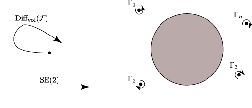
Figure 1.1: The two symmetry groups in the problem of a cylinder interacting with $N$ point vortices are the particle relabelling group $\mathrm{Diff}_{\mathrm{vol}}(\mathcal{F})$ and the Euclidian group $\operatorname{SE}(2)$.

After symplectic reduction with respect to $\mathrm{Diff}_{\mathrm{vol}}(\mathcal{F})$ in section 4, we obtain a dynamical system on the product space $T^{\ast}\operatorname{SE}(2)\times\mathbb{R}^{2N}$, where the first factor is the phase space of the rigid body, while the second factor describes the locations of the point vortices. The dynamics is governed by a magnetic symplectic form: it is the sum of the canonical symplectic forms on both factors, together with a non-canonical interaction term. From a physical point of view, the interaction term embodies the interaction between the point vortices and the rigid body through the ambient fluid. Mathematically speaking, the map associating to each rigid body motion the corresponding motion of the fluid can be viewed as a connection, and the magnetic term is closely related to its curvature.

Note that it is essential here to do symplectic reduction with respect to the particle relabeling symmetry rather than Poisson reduction, even though the latter might be conceptually simpler. Recall that symplectic reduction reduces the system to a co-adjoint orbit; as we shall see below, in the case of fluids interacting with solids these co-adjoint orbits are precisely labelled by the vorticity of the fluid. Symplectic reduction — in particular the selection of one particular level set of the momentum map — therefore amounts to imposing a specific form for the vorticity field. In our case, this is where we introduce the assumption that the vorticity is concentrated in $N$ point vortices. In the case of Poisson reduction, we would have obtained the equations of motion for a rigid body interacting with an arbitrary vorticity field.

After factoring out the particle relabeling symmetry, the resulting dynamical system is invariant under translations and rotations in the plane and can then be reduced with respect to the group $\operatorname{SE}(2)$. This is the subject of section 5. Physically, this corresponds to rewriting the equations of motion obtained after the first reduction in body coordinates. However, because of the presence of the magnetic term in the symplectic form and the fact that $\operatorname{SE}(2)$ acts diagonally on $T^{\ast}\operatorname{SE}(2)\times\mathbb{R}^{2N}$, this is not a straightforward task.

First, we derive the reduced Poisson structure on the reduced space $\mathfrak{se}(2)^{\ast}\times\mathbb{R}^{2N}$. Because of the magnetic contributions to the symplectic form, the reduced Poisson structure is not just the sum of the Poisson structures on the individual factors, but includes certain non-canonical contributions as well. We then show that the momentum map for the $\operatorname{SE}(2)$-symmetry naturally defines a Poisson map taking this Poisson structure into the product Poisson structure, possibly with a cocycle if the momentum map is not equivariant (this happens when the total strength of the point vortices is nonzero). We do the computations for a general product $T^{\ast}H\times P$ first, where $H$ is a Lie group, $P$ is a symplectic manifold, and the product is equipped with a magnetic symplectic form. In this way, we generalize the “coupling to a Lie group” scenario (see Krishnaprasad and Marsden [1987]) to the case where magnetic terms are present.

In this way, the results of SMBK and BMR are put on a firm geometric footing: the BMR Poisson structure is the one obtained through reduction and involves the interaction terms, while the SMBK Poisson structure is simply the product Poisson structure. The Poisson map induced by the $\operatorname{SE}(2)$-momentum map described above turns out to be precisely Shashikanth’s Poisson map. As a consequence, we also obtain an explicit prescription for the symplectic leaves of this system.

Relation with Other Approaches.

Our method consists of rederiving the SMBK and BMR equations by reformulating the motion of a rigid body in a fluid as a geodesic problem on the space $Q$. By imposing the assumption that the vorticity is concentrated in $N$ point vortices, and dividing out the symmetry, we obtain first of all the BMR equations, and secondly (after doing a momentum shift) the SMBK equations. This procedure is worked out in the body of the paper — here we would like to reflect on the similarities with other dynamical systems.

Recall that the dynamics of a particle of charge $e$ in a magnetic field $\mathbf{B}=\nabla\times\mathbf{A}$ can be described in two ways. One is by using canonical variables $(\mathbf{q},\mathbf{p})$ and the Hamiltonian

$$H(\mathbf{q},\mathbf{p})=\frac{1}{2m}\left\|\mathbf{p}-e\mathbf{A}\right\|^{2},$$ (1.3)

while for the other one we use the kinetic energy Hamiltonian $H_{\mathrm{kin}}=\left\|\mathbf{p}\right\|^{2}/2m$ but now we modify the symplectic form to be

$$\Omega_{\mathbf{B}}=\Omega_{\mathrm{can}}+e\mathbf{B}.$$ (1.4)

A simple calculation shows that both systems ultimately give rise to the familiar Lorentz equations. From a mathematical point of view, this can be seen by noting that the momentum shift map $\mathcal{S}:\mathbf{p}\mapsto\mathbf{p}-e\mathbf{A}$ maps the dynamics of the former system into that of the latter:

$$\mathcal{S}^{\ast}\Omega_{\mathbf{B}}=\Omega_{\mathrm{can}}\quad\text{and}\quad\mathcal{S}^{\ast}H_{\mathrm{kin}}=H.$$

In other words, both formulations are related by a symplectic isomorphism, thus making them equivalent.

An over-arching way of looking at the dynamics of a charged particle in a magnetic field is as a geodesic problem (with respect to a certain metric) on a higher-dimensional space: this is part of the famed Kaluza-Klein approach. In this case, spacetime is replaced by the product manifold $\mathbb{R}^{4}\times\operatorname{U}(1)$ and charged particles trace out geodesics on this augmented space. The standard, four-dimensional formulation of the dynamics can then be obtained by dividing out by the internal $\operatorname{U}(1)$-symmetry, resulting in the familiar Lorentz equations on $\mathbb{R}^{4}$. More information about these constructions can be found in Sternberg [1977], Weinstein [1978] and Marsden and Ratiu [1994].

Our approach to the fluid-structure problem is similar but more involved because of the presence of two different symmetry groups. However, the underlying philosophy is the same: by reformulating the motion of a rigid body and the fluid as a geodesic problem on an infinite-dimensional manifold, we follow the philosophy of Kaluza-Klein of trading in the complexities in the equations of motion for an increase in the number of dimensions of the configuration space. Then, by dividing out the $\mathrm{Diff}_{\mathrm{vol}}$-symmetry, we obtain a reduced dynamical system governed by a magnetic symplectic form (the analogue of (1.4)), which is mapped after a suitable momentum shift $\mathcal{S}$ into an equivalent dynamical system governed by the canonical symplectic form but with a modified Hamiltonian. After reducing by the residual $\operatorname{SE}(2)$-symmetry, the former gives rise to the BMR bracket, while the latter is nothing but the SMBK system.

A Note on Integrability.

The case of a circular cylinder is distinguished because of the existence of an additional conservation law, associated with the symmetry that rotates the cylinder around its axis. When the circular cylinder interacts with one external point vortex, a simple count of dimensions and first integrals suggests that this problem is integrable, a fact first proved by Borisov and Mamaev [2003]. Indeed, for a single vortex the phase space is a symplectic leaf of $\mathfrak{se}^{\ast}(2)\times\mathbb{R}^{2}$, which is generically four-dimensional. On the other hand, for the circular cylinder there are two conservation laws: the total energy and the material symmetry associated with rotations around the axis of the cylinder, which hints at Liouville integrability.

In the case of an ellipsoidal cylinder with nonzero eccentricity, Borisov, Mamaev, and Ramodanov [2007] gather numerical evidence to show that the interaction with one vortex is chaotic. This is to be contrasted with the motion of point vortices in an unbounded domain (see Newton [2001]), which is integrable for three vortices or less.

Acknowledgements.

It is a pleasure to thank Richard Montgomery, Paul Newton, Tudor Ratiu and Banavara Shashikanth, as well as Frans Cantrijn, Scott Kelly, Bavo Langerock, Jim Radford, and Clancy Rowley, for useful suggestions and interesting discussions.

J. Vankerschaver is a Postdoctoral Fellow from the Research Foundation – Flanders (FWO-Vlaanderen) and a Fulbright Research Scholar, and wishes to thank both agencies for their support. Additional financial support from the Fonds Professor Wuytack is gratefully acknowledged. E. Kanso’s work is partially supported by NSF through the award CMMI 06-44925. J. E. Marsden is partially supported by NSF Grant DMS-0505711.

2 The Fluid-Solid Problem

This section is subdivided into two parts. In the first, and longest, part we describe the general setup for a planar rigid body interacting with a 2D flow. The second part is then devoted to discussing a number of simplifying assumptions that will make the subsequent developments clearer. By separating these assumptions from the main problem setting, we hope to convince the reader that the method outlined in this paper does not depend on any specific assumptions on the rigid body or the fluid, and can be generalized to more complex problems. At the end of this paper, we discuss how these assumptions can be relaxed.

2.1 General Geometric Setting

Kinematics of a Rigid Body.

Throughout this paper, we consider the motion of a planar rigid body interacting with a 2D flow. We introduce an inertial frame $\mathbf{e}_{1,2,3}$, where $\mathbf{e}_{1,2}$ span the plane of motion and $\mathbf{e}_{3}$ is perpendicular to it. The configuration of the rigid body is then described by a rotation with angle $\beta$ around $\mathbf{e}_{3}$ and a vector $\mathbf{x}_{0}=x_{0}\mathbf{e}_{1}+y_{0}\mathbf{e}_{2}$ describing the location of a fixed point of the body, which we take to be the center of mass.

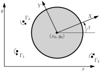
Figure 2.1: The configuration of the rigid body and the point vortices.

The orientation and position $(\beta;x_{0},y_{0})$ determine an element $g$ of the Euclidian group $\operatorname{SE}(2)$ given by

$$g=\begin{pmatrix}R&\mathbf{x}_{0}\\ 0&1\end{pmatrix},\quad\text{where}\,R=\begin{pmatrix}\cos\beta&-\sin\beta\\ \sin\beta&\cos\beta\end{pmatrix}.$$ (2.1)

Written in this way, the group composition and inversion in $\operatorname{SE}(2)$ are given by matrix multiplication and inversion. The Lie algebra of $\operatorname{SE}(2)$ is denoted by $\mathfrak{se}(2)$ and essentially consists of infinitesimal rotations and translations. Its elements are matrices of the form

$$\begin{pmatrix}0&-\Omega&V_{x}\\ \Omega&0&V_{y}\\ 0&0&0\end{pmatrix}.$$

It follows that $\mathfrak{se}(2)$ can be identified with $\mathbb{R}^{3}$ by mapping such a matrix to the triple $(\Omega,V_{x},V_{y})$. We define a basis of $\mathfrak{se}(2)$ given by

$$\mathbf{e}_{\Omega}=\begin{pmatrix}0&-1&0\\ 1&0&0\\ 0&0&0\end{pmatrix},\quad\mathbf{e}_{x}=\begin{pmatrix}0&0&1\\ 0&0&0\\ 0&0&0\end{pmatrix},\quad\mathbf{e}_{y}=\begin{pmatrix}0&0&0\\ 0&0&1\\ 0&0&0\end{pmatrix}.$$ (2.2)

For future reference, we also introduce a moving frame fixed to the rigid body, denoted by $\mathbf{b}_{1,2,3}$. The transformation from body to inertial frame is given by $\mathbf{x}=R\mathbf{X}+\mathbf{x}_{0}$, where $\mathbf{x}=x\mathbf{e}_{1}+y\mathbf{e}_{2}$ and $\mathbf{X}=X\mathbf{b}_{1}+Y\mathbf{b}_{2}$.

The angular and translational velocities of the rigid body relative to the inertial frame are defined as

$$\boldsymbol{\omega}=\dot{\beta}\mathbf{e}_{3}\quad\text{and}\quad\mathbf{v}=\dot{x}_{\circ}\mathbf{e}_{1}+\dot{y}_{\circ}\mathbf{e}_{2},$$ (2.3)

where dots denote derivatives with respect to time. These quantities can be expressed in the body frame: the body angular velocity $\boldsymbol{\Omega}$ and the body translational velocity $\mathbf{V}$ are related to the corresponding inertial quantities by

$$\boldsymbol{\Omega}=\boldsymbol{\omega}\quad\text{and}\quad\mathbf{V}=R^{T}\mathbf{v}.$$ (2.4)

For the case of a planar rigid body, the angular velocity is oriented along the axis perpendicular to the plane and so determines a scalar quantity: $\boldsymbol{\omega}=\omega\mathbf{e}_{3}$ and $\boldsymbol{\Omega}=\Omega\mathbf{b}_{3}$. From a group-theoretic point of view, if the motion of a rigid body is given by a curve $t\mapsto g(t)$ in $\operatorname{SE}(2)$, then we may define an element $\xi(t)\in\mathfrak{se}(2)$ by putting

$$\xi(t)=\frac{d}{d\epsilon}g(t)^{-1}g(t+\epsilon)\Big{|}_{\epsilon=0},$$

and it can easily be checked that $\xi$ coincides with the body angular and translational velocities $(\Omega,\mathbf{V})$.

The kinetic energy of the rigid body is given by the following expression:

$$T_{\mathrm{body}}(\Omega,\mathbf{V})=\frac{\mathbb{I}}{2}\Omega^{2}+\frac{m}{2}\mathbf{V}^{2}$$ (2.5)

where $\mathbb{I}$ is the moment of inertia of the body and $m$ is its mass. The kinetic energy defines an inner product on $\mathfrak{se}(2)$, given by

$$\left\langle\!\left\langle(\Omega_{1},\mathbf{V}_{1}),(\Omega_{2},\mathbf{V}_{2})\right\rangle\!\right\rangle_{\mathfrak{se}(2)}=\begin{pmatrix}\Omega_{1}&\mathbf{V}_{1}\end{pmatrix}\mathbb{M}_{m}\begin{pmatrix}\Omega_{2}\\ \mathbf{V}_{2}\end{pmatrix},$$ (2.6)

for $(\Omega_{1},\mathbf{V}_{1})$ and $(\Omega_{2},\mathbf{V}_{2})$ in $\mathfrak{se}(2)$, and where $\mathbb{M}_{m}$ is given by

$$\mathbb{M}_{m}=\begin{pmatrix}\mathbb{I}&0\\ 0&m\mathbf{I}\end{pmatrix}.$$ (2.7)

Here, $\mathbf{I}$ is the $2$-by-$2$ identity matrix. By left extension, this inner product induces a left-invariant metric on the whole of $\operatorname{SE}(2)$:

$$\left\langle\!\left\langle(g,\dot{g}_{1}),(g,\dot{g}_{2})\right\rangle\!\right\rangle_{\operatorname{SE}(2)}:=\left\langle\!\left\langle g^{-1}\dot{g}_{1},g^{-1}\dot{g}_{2}\right\rangle\!\right\rangle_{\mathfrak{se}(2)},$$ (2.8)

for $(g,\dot{g}_{1})$ and $(g,\dot{g}_{2})$ in $T\operatorname{SE}(2)$.

Incompressible Fluid Dynamics.

The geometric description of an incompressible fluid goes back at least to the work of Arnold [1966], who described the motion of an incompressible fluid in a fixed container $\mathcal{F}$ as a geodesic on the diffeomorphism group of $\mathcal{F}$. In the case of a fluid interacting with a rigid body, the fluid container may change over time, reflecting the fact that the rigid body moves.

Arnold’s formulation can be extended to cover this case by considering the space of embeddings of the reference configuration of the fluid (denoted by $\mathcal{F}_{0}$) into $\mathbb{R}^{2}$. Recall that an embedding $\varphi:\mathcal{F}_{0}\hookrightarrow\mathbb{R}^{2}$ maps each reference point $X\in\mathcal{F}_{0}$ to its current configuration $x=\varphi(X)$. In order to reflect the fact that the fluid is taken to be incompressible, we require that any fluid embedding $\varphi$ is volume preserving: if $d\mathbf{x}$ is the Euclidian area element on $\mathbb{R}^{2}$ and $\eta_{0}$ is a fixed area element on $\mathcal{F}_{0}$, then we require

$$\varphi^{\ast}(d\mathbf{x})=\eta_{0}.$$ (2.9)

The space of all such volume-preserving embeddings is denoted by $\operatorname{Emb}(\mathcal{F}_{0},\mathbb{R}^{2})$. In the sequel, we will specify additional boundary conditions on the fluid configurations, stating for example that the fluid is free to slide along the boundary of the solid, but this does not make any difference for the current expository treatment.

A motion of a fluid is described by a curve $t\mapsto\varphi(t)$ in $\operatorname{Emb}(\mathcal{F}_{0},\mathbb{R}^{2})$. The material velocity field is the tangent vector field $(\varphi_{t},\dot{\varphi}_{t})$ along the curve. Here, $\dot{\varphi}_{t}$ is a map from $\mathcal{F}_{0}$ to $T\mathbb{R}^{2}$, whose value at a point $x\in\mathcal{F}_{0}$ is given by

$$\dot{\varphi}_{t}(x)=\frac{d}{dt}\varphi_{t}(x)\in T_{\varphi(x)}\mathbb{R}^{2}.$$

Note that $\dot{\varphi}_{t}$ is not a vector field in the traditional sense; rather, it is a vector field along the map $\varphi_{t}$. In contrast, the spatial velocity field $\mathbf{u}_{t}$, defined as

$$\mathbf{u}_{t}=\dot{\varphi}_{t}\circ\varphi_{t}^{-1}$$ (2.10)

is a proper vector field, defined on $\varphi_{t}(\mathcal{F}_{0})$.

The motion of a fluid can be described using the kinetic-energy Lagrangian:

$$T_{\mathrm{fluid}}(\varphi,\dot{\varphi})=\frac{\rho}{2}\int_{\mathcal{F}_{t}}\left\|\mathbf{u}\right\|^{2}d\mathbf{x},$$ (2.11)

where $\mathbf{u}$ is the Eulerian velocity field (2.10) and the integration domain is the spatial domain of the fluid at time $t$: $\mathcal{F}_{t}=\varphi_{t}(\mathcal{F}_{0})$. Just as in the case of the rigid body, this kinetic energy induces a metric on the space $\operatorname{Emb}(\mathcal{F}_{0},\mathbb{R}^{2})$, given by

$$\left\langle\!\left\langle\dot{\varphi}_{1},\dot{\varphi}_{2}\right\rangle\!\right\rangle_{\operatorname{Emb}}=\rho\int_{\mathcal{F}_{0}}\dot{\varphi}_{1}\cdot\dot{\varphi}_{2}\,\eta_{0}.$$ (2.12)

By changing variables, this metric can be rewritten in spatial form as follows:

$$\left\langle\!\left\langle\dot{\varphi}_{1},\dot{\varphi}_{2}\right\rangle\!\right\rangle_{\operatorname{Emb}}=\rho\int_{\mathcal{F}_{t}}\mathbf{u}_{1}\cdot\mathbf{u}_{2}\,d\mathbf{x},$$

where $\mathbf{u}_{i}$ is the Eulerian velocity associated to $\dot{\varphi}_{i}$: $\mathbf{u}_{i}=\dot{\varphi}_{i}\circ\varphi_{i}^{-1}$, for $i=1,2$, and the integration is again over the spatial domain $\mathcal{F}_{t}:=\varphi_{t}(\mathcal{F}_{0})$ of the fluid.

The Configuration Space of the Fluid-Solid System.

The motion of a rigid body in an incompressible fluid combines aspects of both rigid-body and fluid dynamics. We assume that the body occupies a circular region $\mathcal{B}_{0}$ in the reference configuration, and that the remainder of the domain, denoted by $\mathcal{F}_{0}$, is taken up by the fluid. The configuration space for the fluid-solid system is made up of pairs $(g,\varphi)\in\operatorname{SE}(2)\times\operatorname{Emb}(\mathcal{F}_{0},\mathbb{R}^{2})$ satisfying the following conditions.

1. The embedding $\varphi$ represents the configuration of the fluid. In particular, $\varphi$ is volume-preserving, i.e. (2.9) is satisfied. In addition, we assume that $\varphi$ approaches the identity at infinity suitably fast.

2. The element $g\in\operatorname{SE}(2)$ describes the configuration of the rigid body.

3. The fluid satisfies a “slip” boundary condition: the normal velocity of the fluid coincides with the normal velocity of the solid, while the tangent velocity can be arbitrary, reflecting the fact that there is no viscosity in the fluid. Mathematically, this boundary condition is imposed by requiring that, as sets, $\varphi(\partial\mathcal{F}_{0})$ is equal to $g(\partial\mathcal{B}_{0})$, where $g\in\operatorname{SE}(2)$ is interpreted as a linear embedding of $\mathcal{B}_{0}$ into $\mathbb{R}^{2}$.

We denote the space of all such pairs as $Q$; this is a submanifold of $\operatorname{SE}(2)\times\operatorname{Emb}(\mathcal{F}_{0},\mathbb{R}^{2})$. The kinetic energy of the fluid-solid system is given by the sum of the rigid-body energy $T_{\mathrm{body}}$ and the kinetic energy $T_{\mathrm{fluid}}$ of the fluid:

$$T =T_{\mathrm{fluid}}+T_{\mathrm{body}}$$

$$=\frac{\rho}{2}\int_{\mathcal{F}_{t}}\left\|\mathbf{u}\right\|^{2}d\mathbf{x}+\frac{\mathbb{I}}{2}\Omega^{2}+\frac{m}{2}\mathbf{V}^{2}.$$ (2.13)

Similarly, there exists a metric on $Q$ given by the sum of the metrics (2.8) and (2.12):

$$\left\langle\!\left\langle(\dot{\varphi}_{1},\dot{g}_{1}),(\dot{\varphi}_{2},\dot{g}_{2})\right\rangle\!\right\rangle=\left\langle\!\left\langle\dot{\varphi}_{1},\dot{\varphi}_{2}\right\rangle\!\right\rangle_{\operatorname{Emb}}+\left\langle\!\left\langle\dot{g}_{1},\dot{g}_{2}\right\rangle\!\right\rangle_{\operatorname{SE}(2)}.$$ (2.14)

The dynamics of rigid bodies moving in perfect fluids was studied before by Kelly [1998], Radford [2003], and Kanso, Marsden, Rowley, and Melli-Huber [2005]; Kanso and Oskouei [2008]. A similar configuration space, but with the $\operatorname{SE}(2)$-factor replaced by a suitable set of smooth manifolds, was studied by Lewis, Marsden, Montgomery, and Ratiu [1986] for the dynamics of a liquid drop.

Particle Relabelling Symmetry.

The kinetic energy $T_{\mathrm{fluid}}$ of the fluid is invariant if we replace $\dot{\varphi}$ by $\dot{\varphi}\circ\phi$, where $\phi$ is a volume-preserving diffeomorphism from $\mathcal{F}_{0}$ to itself. This represents the particle relabelling symmetry referred to in the introduction.

Recall that a diffeomorphism $\phi:\mathcal{F}_{0}\rightarrow\mathcal{F}_{0}$ is volume-preserving if $\phi^{\ast}\eta_{0}=\eta_{0}$, where $\eta_{0}$ is the volume element on $\mathcal{F}_{0}$. The group of all volume-preserving diffeomorphisms is denoted by $\mathrm{Diff}_{\mathrm{vol}}$. This group acts on the right on $\operatorname{Emb}(\mathcal{F}_{0},\mathbb{R}^{2})$ by putting $\varphi\cdot\phi=\varphi\circ\phi$, and hence also on $Q$. The action of $\mathrm{Diff}_{\mathrm{vol}}$ on $Q$ makes $Q$ into the total space of a principal fiber bundle over $\operatorname{SE}(2)$. In other words, if we define the projection $\pi:Q\rightarrow\operatorname{SE}(2)$ as being the projection onto the first factor: $\pi(g,\varphi)=g$, then the fibers of $\pi$ coincide precisely with the orbits of $\mathrm{Diff}_{\mathrm{vol}}$ in $Q$.

Vorticity and Circulation.

In classical fluid dynamics, the vorticity $\boldsymbol{\mu}$ is defined as the curl of the velocity field: $\boldsymbol{\mu}=\nabla\times\mathbf{u}$, and the circulation around the rigid body is the line integral of $\mathbf{u}$ along any curve encircling the rigid body. In two dimensions, $\boldsymbol{\mu}$ can be written as $\boldsymbol{\mu}=\mu\mathbf{e}_{3}$, where $\mu$ is called the scalar vorticity.

According to Noether’s theorem, there is a conserved quantity associated to the particle relabelling symmetry. This conserved quantity turns out to be precisely the circulation of the fluid:

$$\frac{d}{dt}\oint_{\mathcal{C}}\mathbf{u}\cdot d\mathbf{l}=0,$$

and Noether’s theorem hence becomes Kelvin’s theorem, which states that circulation is materially constant. As a consequence of Green’s theorem, the circulation of the fluid is related to the vorticity:

$$\oint_{\mathcal{C}}\mathbf{u}\cdot d\mathbf{l}=\int_{\mathcal{S}}\nabla\times\mathbf{u}\cdot d\mathbf{S},$$

where $\mathcal{S}$ is any surface whose boundary is $\mathcal{C}$. It would lead us too far to explore the geometry of vorticity and circulation in detail (for this, we refer to Arnold and Khesin [1998]) but at this stage we just note that the conservation of vorticity is closely linked to the particle relabelling symmetry.

The Helmholtz-Hodge Decomposition.

If (in addition to being incompressible) the fluid is irrotational, meaning that $\nabla\times\mathbf{u}=0$, then there exists a velocity potential $\Phi$ such that $\mathbf{u}=\nabla\Phi$. In the presence of point vortices, the fluid is not irrotational but the velocity field $\mathbf{u}$ can be uniquely decomposed in an irrotational part and a vector field $\mathbf{u}_{\rm v}$ representing the “rotational” contributions (see for instance Saffman [1992] or Newton [2001]). This is the well-known Helmholtz-Hodge decomposition:

$$\mathbf{u}=\nabla\Phi+\mathbf{u}_{\rm v}.$$ (2.15)

Here, $\mathbf{u}_{\rm v}$ is a divergence-free vector field which is tangent to the boundary of $\mathcal{F}$, while the potential $\Phi$ is the solution to Laplace’s equation $\nabla^{2}\Phi=0$, subject to the boundary conditions that the normal derivative of $\Phi$ equals the normal velocity of the rigid body, and that the velocity vanishes at infinity. In other words, one has

$$\nabla^{2}\Phi=0\quad\text{and}\quad\frac{\partial\Phi}{\partial n}\Big{|}_{\partial\mathcal{F}}=(\boldsymbol{\omega}\times(\mathbf{x}-\mathbf{x}_{0})+\mathbf{v})\cdot\mathbf{n}\quad\text{(for $\mathbf{x}\in\partial\mathcal{F}$)},$$ (2.16)

and $\Phi$ goes to zero as $\left|\mathbf{x}\right|$ goes to infinity. Here $\boldsymbol{\omega}$ and $\mathbf{v}$ are the angular and translational velocity of the rigid body, expressed in a spatial frame, while $\mathbf{x}_{0}$ represents the location of the center of mass.

Since $\Phi$ depends on $\omega$ and $\mathbf{v}$ in a linear way, we may decompose $\Phi$, following Kirchhoff, as

$$\Phi(g,\dot{g};\mathbf{x})=v_{x}\Phi_{x}(g,\mathbf{x})+v_{y}\Phi_{y}(g,\mathbf{x})+\omega\Phi_{\omega}(g,\mathbf{x}).$$ (2.17)

Here $\Phi_{x}$, $\Phi_{y}$, and $\Phi_{\omega}$ are elementary velocity potentials corresponding to infinitesimal translations in the $x$- and $y$-direction and to a rotation, respectively. They satisfy the Laplace equation with the following boundary conditions:

$$\frac{\partial\Phi_{\omega}}{\partial n}=(\mathbf{e}_{3}\times\mathbf{x})\cdot\mathbf{n},\quad\frac{\partial\Phi_{x}}{\partial n}=\mathbf{e}_{1}\cdot\mathbf{n},\quad\text{and}\quad\frac{\partial\Phi_{y}}{\partial n}=\mathbf{e}_{2}\cdot\mathbf{n}.$$

Note that $\Phi$ depends on the boundary data, and hence on $(g,\dot{g})$, while the elementary potentials depend on the location of the rigid body (encoded by $g$) only. For the sake of clarity, we will suppress these arguments when no confusion is possible. The elementary velocity potentials for a circular body are given below: the reader can check that they indeed depend on the location of the rigid body.

The Helmholtz-Hodge decomposition defines a connection on the principal fiber bundle $Q\rightarrow\operatorname{SE}(2)$. To see this, note that any tangent vector to $Q$ is of the form $(g,\dot{g};\varphi,\dot{\varphi})$. We define its horizontal and vertical part by applying the Helmholtz-Hodge decomposition to $\mathbf{u}=\dot{\varphi}\circ\varphi^{-1}$, and we put

$$(g,\dot{g};\varphi,\dot{\varphi})^{H}=(g,\dot{g};\varphi,\nabla\Phi\circ\varphi)\quad\text{and}\quad(g,\dot{g};\varphi,\dot{\varphi})^{V}=(g,0;\varphi,\mathbf{u}_{\rm v}\circ\varphi)$$

We will verify in section 3 below that this prescription indeed defines a connection, which we term the Neumann connection, since its horizontal subspaces are found by solving the Neumann problem (2.16). This connection was used in a variety of contexts, ranging from the dynamics of fluid drops (see Lewis, Marsden, Montgomery, and Ratiu [1986]; Montgomery [2002]) to problems in optimal transport (see Khesin and Lee [2008]).

The Lie Algebra of Divergence-free Vector Fields and its Dual.

At least on a formal level, $\mathrm{Diff}_{\mathrm{vol}}$ is a Lie group with associated to it a Lie algebra, denoted by $\mathfrak{X}_{\mathrm{vol}}$ and consisting of divergence-free vector fields which are parallel to the boundary of $\mathcal{F}_{0}$. The bracket on $\mathfrak{X}_{\mathrm{vol}}$ is the Jacobi-Lie bracket of vector fields (which is the negative of the usual bracket of vector fields) and its dual, denoted by $\mathfrak{X}^{\ast}_{\mathrm{vol}}$, is the set of linear functionals on $\mathfrak{X}_{\mathrm{vol}}$. This set can be identified with the set of one-forms on $\mathcal{F}_{0}$ modulo exact forms:

$$\mathfrak{X}^{\ast}_{\mathrm{vol}}(\mathcal{F}_{0})=\Omega^{1}(\mathcal{F}_{0})/\mathbf{d}\Omega^{0}(\mathcal{F}_{0}),$$

(see Arnold and Khesin [1998]) while the duality pairing between elements of $\mathfrak{X}_{\mathrm{vol}}$ and $\mathfrak{X}^{\ast}_{\mathrm{vol}}$ is given by

$$\left<\mathbf{u},[\alpha]\right>=\int_{\mathcal{F}_{0}}\alpha(\mathbf{u})\,\eta_{0},$$

where $\mathbf{u}\in\mathfrak{X}_{\mathrm{vol}}$ and $[\alpha]\in\mathfrak{X}^{\ast}_{\mathrm{vol}}$. Note that the right-hand side does not depend on the choice of representative $\alpha$.

Another interpretation of the dual Lie algebra $\mathfrak{X}^{\ast}_{\mathrm{vol}}$ is as the set of exact two-forms on $\mathcal{F}_{0}$. Any class $[\alpha]$ in $\mathfrak{X}_{\mathrm{vol}}^{\ast}$ is uniquely determined by the exterior differential $\mathbf{d}\alpha$ and by the value of $\alpha$ on the generators of the first homology of $\mathcal{F}_{0}$. In our case, the first homology group of $\mathcal{F}_{0}$ is generated by any closed curve $\mathcal{C}$ encircling the rigid body, and its pairing with $\alpha$ is given by

$$\Gamma=\int_{\mathcal{C}}\alpha.$$

Under this identification, $\mathbf{d}\alpha$ represents the vorticity, while $\Gamma$ represents the circulation. Since in our case the circulation is assumed to be zero, it follows that $[\alpha]$ is completely determined by $\mathbf{d}\alpha$.

From a geometric point of view, the vorticity field can be interpreted as an element of $\mathfrak{X}_{\mathrm{vol}}^{\ast}$: if we assume that the fluid is moving on an arbitrary Riemannian manifold, then the vorticity can be defined by

$$\mu=\mathbf{d}(\varphi^{\ast}\mathbf{u}^{\flat}).$$

Here $\flat$ is the flat operator associated to the metric. In the case of Euclidian spaces, this definition reduces to the one involving the curl of $\mathbf{u}$. This definition is slightly different from the one in Arnold and Khesin [1998], where vorticity is defined as a two-form on the inertial space $\mathbb{R}^{2}$, whereas in our interpretation, vorticity lives on the material space $\mathcal{F}_{0}$. Both definitions are related by push-forward and pull-back by $\varphi$, and hence carry the same amount of information. Our definition has the advantage that $\mu$ is naturally an element of $\mathfrak{X}_{\mathrm{vol}}^{\ast}$, which is preferable from a geometric point of view.

We finish this section by noting that any Lie group acts on its Lie algebra and its dual Lie algebra through the adjoint and the co-adjoint action, respectively. For the group of volume-preserving diffeomorphisms, both are given by pull-back: if $\phi$ is an element of $\mathrm{Diff}_{\mathrm{vol}}$, and $\mathbf{u}$ and $\mathbf{d}\alpha$ are elements of $\mathfrak{X}_{\mathrm{vol}}$ and $\mathfrak{X}_{\mathrm{vol}}^{\ast}$, respectively, then

$$\mathrm{Ad}_{\phi}(\mathbf{u})=\phi^{\ast}\mathbf{u}\quad\text{and}\quad\mathrm{CoAd}_{\phi}(\mathbf{d}\alpha)=\mathbf{d}(\phi^{\ast}\alpha).$$

2.2 Point Vortices Interacting with a Circular Cylinder

In this section, we impose some specific assumptions on the rigid body and the fluid. It should be pointed out that while these assumptions greatly simplify the exposition, the general reduction procedure can be carried out under far less stringent assumptions. Later on, we will discuss how some of these assumptions may be removed.

The Rigid Body.

In order to tie in this work with previous research efforts, we assume the rigid body to be circular with radius $R$ and neutrally buoyant (i.e. its body weight $m$ is balanced by the force of buoyancy). If the density of the fluid is set to $\rho=1$, this implies that the body has mass $m=\pi R^{2}$. The moment of inertia of the body around the axis of symmetry is denoted by $\mathbb{I}$.

For a rigid planar body of circular shape, the elementary velocity potentials $\Phi_{x}$, $\Phi_{y}$, and $\Phi_{\omega}$ occurring in (2.17) can be calculated analytically (see Lamb [1945]) and are given by

$$\Phi_{x}=-R\frac{x-x_{0}}{(x-x_{0})^{2}+(y-y_{0})^{2}},\quad\text{and}\quad\Phi_{y}=-R\frac{y-y_{0}}{(x-x_{0})^{2}+(y-y_{0})^{2}},$$ (2.18)

while $\Phi_{\omega}=0$, reflecting the rotational symmetry of the body. Here $(x_{0},y_{0})$ are the coordinates of the center of the disc.

In some cases, it will be more convenient to express $\Phi$ in body coordinates. In analogy with (2.17), we may write

$$\Phi(g,\dot{g},\mathbf{X})=V_{x}\Phi_{X}(\mathbf{X})+V_{y}\Phi_{Y}(\mathbf{X})+\Omega\Phi_{\Omega}(\mathbf{X}),$$

where $(V_{x},V_{y})$ and $\Omega$ are the translational and angular velocity in the body frame, respectively. For the circular cylinder, the elementary potentials in body frame are given by

$$\Phi_{X}=-R\frac{X}{X^{2}+Y^{2}},\quad\Phi_{Y}=-R\frac{Y}{X^{2}+Y^{2}}\quad\text{and}\quad\Phi_{\Omega}=0.$$ (2.19)

Note that $\Phi_{X},\Phi_{Y}$ and $\Phi_{\Omega}$ do not depend on the location of the rigid body, in contrast to $\Phi_{x},\Phi_{y}$ and $\Phi_{\omega}$.

Point Vortices.

As for the fluid, we make the fundamental assumption that the vorticity is concentrated in $N$ point vortices of strengths $\Gamma_{i}$, $i=1,\ldots,N$, and that there is no circulation. Considered as a two-form on $\mathcal{F}_{0}$, the former means that the vorticity is given by

$$\mu=\sum_{i=1}^{N}\Gamma_{i}\delta(\bar{\mathbf{x}}-\bar{\mathbf{x}}_{i})\mathbf{d}\bar{x}\wedge\mathbf{d}\bar{y},$$ (2.20)

where $(\bar{x},\bar{y})$ are coordinates on $\mathcal{F}_{0}$, and $\bar{\mathbf{x}}_{i}$ is the reference location of the $i$th vortex, $i=1,\ldots,N$. As pointed out above, $\mu$ is an element of $\mathfrak{X}_{\mathrm{vol}}^{\ast}$.

The Kirchhoff-Routh Function.

Shashikanth, Marsden, Burdick, and Kelly [2002] showed that the kinetic energy for the vortex system is the negative of the Kirchhoff-Routh function $W_{G}$ for a system of $N$ point vortices moving in a domain with moving boundaries:

$$T_{\mathrm{vortex}}(\mathbf{X}_{1},\ldots,\mathbf{X}_{N})=-W_{G}(\mathbf{X}_{1},\ldots,\mathbf{X}_{N}).$$ (2.21)

The precise form of $W_{G}$ is given by

$$W_{G}(\mathbf{X}_{1},\ldots,\mathbf{X}_{N})=\sum_{i,j(i>j)}\Gamma_{i}\Gamma_{j}G(\mathbf{X}_{i},\mathbf{X}_{j})+\frac{1}{2}\sum_{i}\Gamma_{i}g(\mathbf{X}_{i},\mathbf{X}_{i}),$$ (2.22)

where $G(\mathbf{X}_{0},\mathbf{X}_{1})$ is a Green’s function for the Laplace operator of the form

$$G(\mathbf{X}_{0},\mathbf{X}_{1})=g(\mathbf{X}_{0},\mathbf{X}_{1})+\frac{1}{4\pi}\log\left\|\mathbf{X}_{0}-\mathbf{X}_{1}\right\|^{2}.$$ (2.23)

The function $g$ is harmonic in the fluid domain and is the stream function of $\mathbf{u}_{I}$. As pointed out in Shashikanth, Marsden, Burdick, and Kelly [2002], in the case of a circular cylinder, $g$ can be calculated explicitly using Milne-Thomson’s circle theorem (Milne-Thomson [1968]), and is given by

$$g(\mathbf{X},\mathbf{Y})=\frac{1}{4\pi}\log\left\|\mathbf{X}\right\|^{2}-\frac{1}{4\pi}\log\left\|\mathbf{X}-\frac{R^{2}}{\left\|\mathbf{Y}\right\|^{2}}\mathbf{Y}\right\|^{2}.$$

From a geometrical point of view, Marsden and Weinstein [1983] showed that the vortex energy can be obtained (up to some “self-energy” terms) by inverting the relation $\mu=\nabla\times\mathbf{u}$, where $\mu$ is the scalar part of (2.20), and substituting the resulting velocity field $\mathbf{u}$ generated by $N$ vortices into the expression for the kinetic energy of the fluid. Although the analysis of Marsden and Weinstein [1983] was for an unbounded fluid domain, their result can easily be extended to the case considered here, yielding again the negative of the Kirchhoff-Routh function as in (2.21).

Dynamics of the Fluid-Solid System.

As stated in the introduction, Shashikanth, Marsden, Burdick, and Kelly [2002] (SMBK) were the first to derive the equations of motion for a rigid cylinder interacting with $N$ point vortices. These equations generalize both the Kirchhoff equations for a rigid body in a potential flow and the equations for $N$ point vortices in a bounded flow. Rather remarkably, SMBK established by direct inspection that these equations are Hamiltonian with respect to the canonical Poisson structure on $\mathfrak{se}(2)^{\ast}\times\mathbb{R}^{2N}$ (i.e. the sum of the Poisson structures on both factors), and a Hamiltonian given below involving the kinetic energy and interaction terms.

The SMBK equations are given by

$$\frac{d\mathbf{L}}{dt}=0,\quad\frac{d\mathbf{A}}{dt}+\mathbf{V}\times\mathbf{L}=0,\quad\text{and}\quad\Gamma_{k}\frac{d\mathbf{X}_{k}}{dt}=-J\frac{\partial H}{\partial\mathbf{X}_{k}},$$ (2.24)

where $\mathbf{L}$ and $\mathbf{A}=A\mathbf{e}_{3}$ are the translational and angular momenta of the system, defined by

$$\mathbf{L} =c\mathbf{V}+\sum_{k=1}^{N}\Gamma_{k}\mathbf{X}_{k}\times\mathbf{e}_{3}+\sum_{k=1}^{N}\Gamma_{k}\mathbf{e}_{3}\times\frac{\mathbf{X}_{k}}{\left\|\mathbf{X}_{k}\right\|^{2}}$$ (2.25)

$$A =\mathbb{I}\Omega-\frac{1}{2}\sum_{i=1}^{N}\Gamma_{i}\left\|\mathbf{X}_{i}\right\|^{2},$$

and $H$ is the Hamiltonian:

$$H(\mathbf{L},\mathbf{X}_{k}) =-W(\mathbf{L},\mathbf{X}_{k})+\frac{1}{2c}\left\|\mathbf{L}\right\|^{2}-\frac{1}{c}\Big{(}\sum\Gamma_{k}(\mathbf{L}\times\mathbf{X}_{k})\cdot\mathbf{e}_{3}$$

$$-\frac{1}{2}\sum\Gamma_{k}^{2}\left\|\mathbf{X}_{k}\right\|^{2}-\sum_{j>k}\Gamma_{k}\Gamma_{j}\mathbf{X}_{k}\cdot\mathbf{X}_{j}$$ (2.26)

$$+\frac{1}{2}\left<\sum\Gamma_{k}\frac{\mathbf{X}_{k}}{\left\|\mathbf{X}_{k}\right\|^{2}},\sum\Gamma_{k}\frac{\mathbf{X}_{k}}{\left\|\mathbf{X}_{k}\right\|^{2}}\right>\Big{)}.$$

Here, $c$ is the total mass of the cylinder, consisting of the intrinsic mass $m$ and the added mass $\pi R^{2}$ (due to the presence of the fluid): $c=m+\pi R^{2}=2\pi R^{2}$.

Theorem 2.1.

The SMBK equations are Hamiltonian on the space $\mathfrak{se}(2)^{\ast}\times\mathbb{R}^{2N}$ equipped with the Poisson bracket

$$\{F,G\}_{\mathfrak{se}(2)^{\ast}\times\mathbb{R}^{2N}}=\{F_{|\mathfrak{se}(2)^{\ast}},G_{|\mathfrak{se}(2)^{\ast}}\}_{\mathrm{l.p}}+\{F_{|\mathbb{R}^{2N}},G_{|\mathbb{R}^{2N}}\}_{\mathrm{vortex}}.$$ (2.27)

Here, $F$ and $G$ are functions on $\mathfrak{se}(2)^{\ast}\times\mathbb{R}^{2N}$.

In the theorem above, $\{\cdot,\cdot\}_{\mathrm{l.p}}$ is the Lie-Poisson bracket on $\mathfrak{se}(2)^{\ast}$:

$$\{f_{1},f_{2}\}_{\mathfrak{se}(2)^{\ast}}=(\nabla f_{1})^{T}\Lambda\nabla f_{2},\quad\text{where}\quad\Lambda=\begin{pmatrix}0&-P_{y}&P_{x}\\ P_{y}&0&0\\ -P_{x}&0&0\end{pmatrix},$$ (2.28)

for arbitrary functions $f_{1},f_{2}$ on $\mathfrak{se}(2)^{\ast}$. Similarly, $\{\cdot,\cdot\}_{\mathrm{vortex}}$ is the vortex bracket, given by:

$$\{g_{1},g_{2}\}_{\mathrm{vortex}}=\sum_{i=1}^{N}\frac{1}{\Gamma_{i}}\left(\frac{\partial g_{1}}{\partial X_{i}}\frac{\partial g_{2}}{\partial Y_{i}}-\frac{\partial g_{2}}{\partial X_{i}}\frac{\partial g_{1}}{\partial Y_{i}}\right),$$ (2.29)

where $g_{1},g_{2}$ are arbitrary functions on $\mathbb{R}^{2N}$.

The BMR Equations.

A completely different perspective on the rigid body interacting with $N$ point vortices is offered by Borisov, Mamaev, and Ramodanov [2003] (BMR). From their point of view, the equations of motion are again written in Hamiltonian form on $\mathfrak{se}(2)^{\ast}\times\mathbb{R}^{2N}$, but now with a noncanonical Poisson bracket:

$$\dot{F}=\{F,H\}_{\mathrm{BMR}}$$

for all functions $F$ on $\mathfrak{se}(2)^{\ast}\times\mathbb{R}^{2N}$. The Hamiltonian is the sum of the kinetic energies of the subsystems, without interaction terms:

$$H=\frac{c}{2}\left<\mathbf{V},\mathbf{V}\right>-W_{G}(\mathbf{V},\mathbf{X}_{k}),$$

whereas the Poisson bracket is determined by its value on the coordinate functions:

$$\{V_{1},V_{2}\}_{\mathrm{BMR}} =\frac{\Gamma}{c^{2}}-\sum\frac{\Gamma}{c^{2}}\frac{R_{i}^{4}-R^{4}}{R_{i}^{4}},\, \{V_{1},X_{i}\}_{\mathrm{BMR}} =\frac{1}{c}\frac{R_{i}^{4}-R^{2}(X_{i}^{2}-Y_{i}^{2})}{R_{i}^{4}},$$

$$\{V_{1},Y_{i}\}_{\mathrm{BMR}} =-\frac{2R^{2}}{c}\frac{X_{i}Y_{i}}{R_{i}^{4}}, \{V_{2},X_{i}\}_{\mathrm{BMR}} =-\frac{2R^{2}}{c}\frac{X_{i}Y_{i}}{R_{i}^{4}},$$ (2.30)

$$\{V_{2},Y_{i}\}_{\mathrm{BMR}} =\frac{1}{c}\frac{R_{i}^{4}+R^{2}(X_{i}^{2}-Y_{i}^{2})}{R_{i}^{4}}, \{X_{i},Y_{i}\}_{\mathrm{BMR}} =-\frac{1}{\Gamma_{i}},$$

where $R_{i}^{2}=\left\|\mathbf{X}_{i}\right\|^{2}$, $\mathbf{V}=(V_{1},V_{2})$, $\mathbf{X}_{i}=(X_{i},Y_{i})$, and $\Gamma$ is the total vortex strength:

$$\Gamma=\sum_{i=1}^{N}\Gamma_{i}.$$

Note that this Poisson bracket differs from the one in Borisov, Mamaev, and Ramodanov [2003] by an overall factor of $2\pi$. Shashikanth [2005] showed that this discrepancy can be attributed to the way in which BMR choose the fluid density.

The Link between the SMBK and the BMR Equations.

By explicit calculation, Shashikanth [2005] constructed a Poisson map taking the SMBK equations into the BMR equations. His result is listed below.

Theorem 2.2.

The map $\mathcal{S}:(\mathbf{L},A;\mathbf{X}_{1},\ldots,\mathbf{X}_{N})\mapsto(\mathbf{V},\Omega;\mathbf{X}_{1},\ldots,\mathbf{X}_{N})$, where $\mathbf{L}$ and $A$ are given by (2.25), is a Poisson map from $\mathfrak{se}(2)^{\ast}\times\mathbb{R}^{2N}$ equipped with the bracket $\{\cdot,\cdot\}_{\mathfrak{se}(2)^{\ast}\times\mathbb{R}^{2N}}$ to $\mathfrak{se}(2)^{\ast}\times\mathbb{R}^{2N}$ with the bracket $\{\cdot,\cdot\}_{\mathrm{BMR}}$.

Even though this result asserts that both sets of equations are equivalent, it leaves open the question as to why this is so. By re-deriving the equations of motion using symplectic reduction, not only do we obtain both sets of equations, but the map $\mathcal{S}$ also follows naturally.

3 The Neumann Connection

The bundle $\pi:Q\rightarrow\operatorname{SE}(2)$ is equipped with a principal fibre bundle connection, called the Neumann connection by Montgomery [1986]. There are many ways of describing this connection, but from a physical point of view, the definition using the horizontal lift operator is perhaps most appealing. From this point of view, the Neumann connection is a map

$$\mathbf{h}:Q\times T\operatorname{SE}(2)\rightarrow TQ,\quad\mathbf{h}(\varphi,g,\dot{g})=\nabla\Phi\circ\varphi,$$ (3.1)

where $\Phi$ is the solution of the Neumann problem (2.16) associated to $(g,\dot{g})$. In other words, the Neumann connection associates to each motion $(g,\dot{g})$ the corresponding induced velocity field of the fluid, and hence encodes the effect of the body on the fluid. It is important to note that the Neumann connection does not depend on the point vortex model and is valid for any vorticity field.

Similar connections as this one have been described before (see for example Lewis, Marsden, Montgomery, and Ratiu [1986]; Khesin and Lee [2008]) but a complete overview of its definition and properties seems to be lacking. In this section, we give an outline of the properties of the Neumann connection which are relevant for the developments in this paper, leaving detailed proofs for the appendix.

Invariance of the Kirchhoff Decomposition.

Before introducing the Neumann connection, we prove that the velocity potential $\Phi(g,\dot{g};\mathbf{x})$ is left $\operatorname{SE}(2)$-invariant, expressing the fact that the dynamics is invariant under translations and rotations of the combined solid-fluid system.

Proposition 3.1.

The velocity potential $\Phi$ is left $\operatorname{SE}(2)$-invariant in the sense that

$$\Phi(hg,TL_{h}(\dot{g});h\mathbf{x})=\Phi(g,\dot{g};\mathbf{x})$$ (3.2)

for all $h\in\operatorname{SE}(2)$ and $(g,\dot{g};\mathbf{x})\in T\operatorname{SE}(2)\times\mathbb{R}^{2}$.

Proof.

This assertion can be proved in a number of different ways. The easiest is to use the assumption that the body is circular and solve the equation for the elementary potentials explicitly. Recall that these elementary potentials are given by (2.18). It is then straightforward to check that (3.2) holds, using the transformation properties of the velocity in the inertial frame. ∎

The Connection One-form.

For our purposes, it is convenient to define the Neumann connection through its connection one-form $\mathcal{A}:TQ\rightarrow\mathfrak{X}_{\mathrm{vol}}$ given by

$$\mathcal{A}_{(\varphi,g)}(\dot{g},\dot{\varphi})=\varphi^{\ast}\mathbf{u}_{\rm v},$$ (3.3)

where $\mathbf{u}_{\rm v}$ is the divergence-free part in the Helmholtz-Hodge decomposition (2.15) of the Eulerian velocity $\mathbf{u}=\dot{\varphi}\circ\varphi^{-1}$. A proof that this prescription determines a well-defined connection form can be found in the appendix, proposition A.1, where it is also shown that this prescription agrees with the horizontal lift operator (3.1).

The Curvature of the Neumann Connection.

It will be convenient in what follows to have an expression for the $\mu$-component of the curvature of the Neumann connection, where for now $\mu$ is an arbitrary element of $\mathfrak{X}_{\mathrm{vol}}^{\ast}$. Later on, $\mu$ will be the vorticity (2.20) associated to $N$ point vortices.

The curvature of a principal fiber bundle connection is a two-form $\mathcal{B}$ whose definition is listed in the appendix. For the Neumann connection we have

$$\mathcal{B}_{(g,\varphi)}((\dot{g}_{1},\dot{\varphi}_{1}),(\dot{g}_{2},\dot{\varphi}_{2}))=-\mathcal{A}_{(g,\varphi)}([X^{H},Y^{H}]),$$ (3.4)

where $X^{H}$ and $Y^{H}$ are horizontal vector fields on $Q$ such that $X^{H}(g,\varphi)=(\dot{g}_{1},\dot{\varphi}_{1})$ and $Y^{H}(g,\varphi)=(\dot{g}_{2},\dot{\varphi}_{2})$.

Proposition 3.2.

Let $(\dot{g}_{1},\dot{\varphi}_{1})$ and $(\dot{g}_{2},\dot{\varphi}_{2})$ be elements of $T_{(g,\varphi)}Q$ and denote the solutions of the Neumann problem (2.16) associated to $(g,\dot{g}_{1})$ resp. $(g,\dot{g}_{2})$ by $\Phi_{1}$ and $\Phi_{2}$. Then the $\mu$-component of the curvature $\mathcal{B}$ is given by

$$\left<\mu,\mathcal{B}_{(g,\varphi)}((\dot{g}_{1},\dot{\varphi}_{1}),(\dot{g}_{2},\dot{\varphi}_{2}))\right>=\left\langle\!\left\langle\mu,\mathbf{d}\Phi_{1}\wedge\mathbf{d}\Phi_{2}\right\rangle\!\right\rangle_{\mathcal{F}}-\int_{\partial\mathcal{F}}\alpha\wedge\ast(\mathbf{d}\Phi_{1}\wedge\mathbf{d}\Phi_{2}),$$ (3.5)

where $\left\langle\!\left\langle\cdot,\cdot\right\rangle\!\right\rangle_{\mathcal{F}}$ is the metric on the space of forms on $\mathcal{F}$, induced by the Euclidian metric on $\mathcal{F}$.

Proof.

Let $\mu$ be equal to $\varphi^{\ast}\mathbf{d}\alpha$, and pick $\alpha$ such that $\alpha=\mathbf{u}_{\rm v}^{\flat}$, where $\mathbf{u}_{\rm v}$ is a divergence-free vector field on $\mathcal{F}$ tangent to $\partial\mathcal{F}$. For example, in the case of the vorticity due to $N$ point vortices, $\mathbf{u}_{\rm v}$ is the velocity field due to the vortices and their images (see Saffman [1992]). The calculation of the curvature involves computing the Jacobi-Lie bracket of two horizontal vector fields and taking the divergence-free part of the result. Because of the special form of $\alpha$ we can dispense with the latter step, since $\alpha$ is chosen to be $L_{2}$-orthogonal to gradient vector fields. Therefore, the $\mu$-component of the curvature is given by

$$\left<\mu,\mathcal{B}_{(g,\varphi)}((\dot{g}_{1},\dot{\varphi}_{1}),(\dot{g}_{2},\dot{\varphi}_{2}))\right> =-\left<\mu,\mathcal{A}_{(g,\varphi)}([X^{H},Y^{H}])\right>$$

$$=-\int_{\mathcal{F}_{0}}(\varphi^{\ast}\alpha)([X^{H},Y^{H}])\,\eta_{0},$$

where the bracket on the left-hand side is the Jacobi-Lie bracket, which is the negative of the usual commutator of vector fields.

The bracket can be made more explicit by noting that (as vector fields on $Q$)

$$[X^{H},Y^{H}](g,\varphi)=([(\mathbf{d}\Phi_{1})^{\flat},(\mathbf{d}\Phi_{2})^{\flat}]\circ\varphi,\cdots),$$

where the dots denote a term in $T_{g}\operatorname{SE}(2)$ whose explicit form doesn’t matter. The curvature then becomes

$$\left<\mu,\mathcal{B}_{(g,\varphi)}((\dot{g}_{1},\dot{\varphi}_{1}),(\dot{g}_{2},\dot{\varphi}_{2}))\right>=-\int_{\mathcal{F}}\alpha([(\mathbf{d}\Phi_{1})^{\flat},(\mathbf{d}\Phi_{2})^{\flat}])\,d\mathbf{x}.$$

The remainder of the proof relies on the following formula for the codifferential of a wedge product (Vaisman [1994, formula 1.34]):

$$\delta(\alpha\wedge\beta)=\delta\alpha\wedge\beta+(-1)^{p}\alpha\wedge\delta\beta-[\alpha^{\flat},\beta^{\flat}]^{\sharp},$$ (3.6)

where $p=\deg\alpha$. Applying (3.6) with $\alpha=\mathbf{d}\Phi_{1}$ and $\beta=\mathbf{d}\Phi_{2}$ gives

$$[(\mathbf{d}\Phi_{1})^{\flat},(\mathbf{d}\Phi_{2})^{\flat}]^{\sharp}=\Delta\Phi_{1}\mathbf{d}\Phi_{2}-\Delta\Phi_{2}\mathbf{d}\Phi_{1}-\delta(\mathbf{d}\Phi_{1}\wedge\mathbf{d}\Phi_{2}),$$

where $\Delta$ is the Laplace-Beltrami operator on differential forms. Since both $\Phi_{1}$ and $\Phi_{2}$ are harmonic, the first two terms of the right-hand side vanish. Consequently, the $\mu$-component of the curvature becomes

$$\left<\mu,\mathcal{B}_{(g,\varphi)}((\dot{g}_{1},\dot{\varphi}_{1}),(\dot{g}_{2},\dot{\varphi}_{2}))\right> =\left\langle\!\left\langle\alpha,\delta(\mathbf{d}\Phi_{1}\wedge\mathbf{d}\Phi_{2})\right\rangle\!\right\rangle_{\mathcal{F}}$$

$$=\left\langle\!\left\langle\mathbf{d}\alpha,\mathbf{d}\Phi_{1}\wedge\mathbf{d}\Phi_{2}\right\rangle\!\right\rangle_{\mathcal{F}}-\int_{\partial\mathcal{F}}\alpha\wedge\ast(\mathbf{d}\Phi_{1}\wedge\mathbf{d}\Phi_{2}),$$

using the adjointness of $\mathbf{d}$ and $\delta$ for manifolds with boundary (this is a simple consequence of Stokes’ theorem). ∎

In traditional fluid mechanics notation, formula (3.5) becomes

$$\left<\mu,\mathcal{B}\right>=\int_{\mathcal{F}}(\nabla\times\mathbf{u}_{V})\cdot(\nabla\Phi_{1}\times\nabla\Phi_{2})dx-\int_{\partial\mathcal{F}}\mathbf{u}_{V}\cdot(\mathbf{n}\times(\nabla\Phi_{1}\times\nabla\Phi_{2}))dA,$$

a formula first derived in Montgomery [1986].

4 Reduction with Respect to the Diffeomorphism Group

As mentioned in the introduction, the fluid-solid system on the space $Q\subset\operatorname{SE}(2)\times\operatorname{Emb}(\mathcal{F}_{0},\mathbb{R}^{2})$ is invariant under the particle relabelling group $\mathrm{Diff}_{\mathrm{vol}}$. We now perform symplectic reduction to eliminate that symmetry. In order to do so, we need to fix a value of the momentum map associated to the $\mathrm{Diff}_{\mathrm{vol}}$-symmetry. From a physical point of view, this boils down to fixing the vorticity of the system; it is at this point that the assumption is used that the vorticity is concentrated in $N$ point vortices.

Before tackling symplectic reduction in the context of the fluid-solid system, we first give a general overview of cotangent bundle reduction following Marsden, Misiołek, Ortega, Perlmutter, and Ratiu [2007]. Roughly speaking, applying symplectic reduction to a cotangent bundle yields a space which is diffeomorphic to the product of a reduced cotangent bundle and a co-adjoint orbit of the group. The dynamics on the reduced space is governed by a reduced Hamiltonian and a magnetic symplectic form: the reduced symplectic form is the sum of the canonical symplectic forms on the individual factors and an additional magnetic term.

As we shall see below, in the case of the fluid-solid system, the reduced phase space is equal to $T^{\ast}\operatorname{SE}(2)\times\mathbb{R}^{2N}$, where the first factor describes the rigid body, while the second factor determines the configuration of the vortices. At first sight, it may therefore appear that the intermediate fluid is completely gone. Yet, the vortices act on the rigid body, and vice versa, through the surrounding fluid. The answer to this apparent contradiction is that the effect of the fluid is concentrated in the magnetic symplectic form, for which we derive a convenient expression below.

4.1 Cotangent Bundle Reduction: Review

In this section, we collect some relevant results from Marsden, Misiołek, Ortega, Perlmutter, and Ratiu [2007]. We consider a manifold $Q$ on which a Lie group $G$, with Lie algebra $\mathfrak{g}$, acts from the right and we denote the action by $\sigma:Q\times G\rightarrow Q$. In addition, we assume that we are given a connection one-form $\mathcal{A}:TQ\rightarrow\mathfrak{g}$ with curvature two-form $\mathcal{B}$. In the rest of this paper, $Q$ will be the configuration space of the solid-fluid system, while the structure group $G$ will be $\mathrm{Diff}_{\mathrm{vol}}$, and the connection $\mathcal{A}$ the Neumann connection.

The Curvature as a Two-form on the Reduced Space.

Let $\mu$ be an element of $\mathfrak{g}^{\ast}$, and denote its isotropy subgroup under the co-adjoint action by $G_{\mu}$:

$$G_{\mu}=\left\{g\in G:\mathrm{CoAd}_{g}\mu=\mu\right\}.$$

Consider the contraction $\left<\mu,\mathcal{B}\right>$ of $\mu$ with the curvature $\mathcal{B}$: due to the $G$-equivariance and the fact that $\mathcal{B}$ vanishes on vertical vectors (see (A.2)), we may show that $\left<\mu,\mathcal{B}\right>$ is a $G_{\mu}$-invariant form.

Proposition 4.1.

The $\mu$-component of the curvature $\mathcal{B}$ is a $G_{\mu}$-invariant two-form:

1. $\sigma^{\ast}_{g}\left<\mu,\mathcal{B}\right>=\left<\mu,\mathcal{B}\right>$, for all $g\in G_{\mu}$;

2. $i_{\xi_{Q}}\left<\mu,\mathcal{B}\right>=0$ for all $\xi\in\mathfrak{g}_{\mu}$.

Hence, $\left<\mu,\mathcal{B}\right>$ induces a two-form $\bar{\mathcal{B}}_{\mu}$ on $Q/G_{\mu}$ such that

$$\pi_{Q,G_{\mu}}^{\ast}\bar{\mathcal{B}}_{\mu}=\left<\mu,\mathcal{B}\right>,$$

where $\pi_{Q,G_{\mu}}:Q\rightarrow Q/G_{\mu}$ is the quotient map.

Proof.

For the first property, we have

$$\sigma^{\ast}_{g}\left<\mu,\mathcal{B}\right>=\left<\mu,\sigma_{g}^{\ast}\mathcal{B}\right>=\left<\mu,\mathrm{Ad}_{g^{-1}}\mathcal{B}\right>=\left<\mathrm{CoAd}_{g}(\mu),\mathcal{B}\right>=\left<\mu,\mathcal{B}\right>$$

if $g\in G_{\mu}$. The second item follows from the corresponding property for $\mathcal{B}$. Actually, more is true: $i_{\xi_{Q}}\left<\mu,\mathcal{B}\right>=0$ for all $\xi\in\mathfrak{g}$, not just in $\mathfrak{g}_{\mu}$. ∎

Cotangent Bundle Reduction.

The first stage in reducing the phase space consists of dividing out the particle relabelling symmetry. To this end, we use the framework of cotangent bundle reduction to construct the reduced phase space. The framework for cotangent bundle reduction outlined in Marsden, Misiołek, Ortega, Perlmutter, and Ratiu [2007] allows us to write down the reduced phase space and the modified symplectic form. We quote:

Theorem 4.2.

(Marsden et al. [theorem 2.2.1])

1. There exists a symplectic imbedding $\varphi_{\mu}$ of the reduced phase space $(T^{\ast}Q)_{\mu}$ into the cotangent bundle $T^{\ast}(Q/G_{\mu})$ with the shifted symplectic structure $\Omega_{\mathcal{B}}:=\Omega_{\mathrm{can}}-B_{\mu}$.

2. The image of $\varphi_{\mu}$ is the vector subbundle $[T\pi_{Q,G_{\mu}}(V)]^{\circ}$ of $T^{\ast}(Q/G_{\mu})$, where $V\subset TQ$ is the vector subbundle consisting of vectors tangent to the $G$-orbits in $Q$, and ^∘ denotes the annihilator relative to the natural duality pairing between $T(Q/G_{\mu})$ and $T^{\ast}(Q/G_{\mu})$.

Here $(T^{\ast}Q)_{\mu}$ is the reduced phase space $J^{-1}(\mu)/G_{\mu}$, where $G_{\mu}$ is the isotropy subgroup of $\mu$. The two-form $B_{\mu}$ is called the magnetic two-form, and is defined as $B_{\mu}=\pi_{Q/G_{\mu}}^{\ast}\beta_{\mu}$, where $\pi_{Q/G_{\mu}}:T^{\ast}(Q/G_{\mu})\rightarrow Q/G_{\mu}$ is the cotangent bundle projection and $\beta_{\mu}$ is a two-form on $Q/G_{\mu}$.

To define $\beta_{\mu}$, consider the one-form $\alpha_{\mu}:=\left<\mu,\mathcal{A}\right>$ on $Q$. One can show that $\mathbf{d}\alpha_{\mu}$ (but not $\alpha_{\mu}$ itself) is $G_{\mu}$-invariant, and the induced two-form on $Q/G_{\mu}$ is precisely $\beta_{\mu}$, or in other words

$$\pi^{\ast}_{Q,G_{\mu}}\beta_{\mu}=\mathbf{d}\alpha_{\mu},$$

where $\pi_{Q,G_{\mu}}:Q\rightarrow Q/G_{\mu}$ is the quotient map. The calculation of $\mathbf{d}\alpha_{\mu}$ is greatly facilitated by using the Cartan structure equation (Kobayashi and Nomizu [1963]), which allows us to rewrite $\mathbf{d}\alpha_{\mu}$ as

$$\mathbf{d}\alpha_{\mu}=\left<\mu,\mathcal{B}\right>-\left<\mu,[\mathcal{A},\mathcal{A}]\right>.$$ (4.1)

Observe the sign difference on the right-hand side with Marsden, Misiołek, Ortega, Perlmutter, and Ratiu [2007], which is due to the fact that we take $G$ to be acting on $Q$ from the right.

4.2 The Reduced Phase Space

Theorem 4.2 provides us with an explicit prescription for the reduced phase space. Recall that the diffeomorphism group $\mathrm{Diff}_{\mathrm{vol}}$ acts on the dual Lie algebra $\mathbf{d}\Omega^{1}(\mathcal{F}_{0})$ through pull-back. In particular, if $\mu$ represents the vorticity due to $N$ point vortices as in (2.20), then

$$\phi^{\ast}\mu=\sum_{i=1}^{N}\Gamma_{i}\delta(\mathbf{\bar{x}}-\phi^{-1}(\mathbf{\bar{x}}_{i}))\,\mathbf{d}\bar{x}\wedge\mathbf{d}\bar{y}.$$

In other words, the diffeomorphism group acts on the space of point vortices by simply moving the vortices. It also follows that the isotropy subgroup of $\mu$ consists of all diffeomorphisms $\phi$ for which the vortex reference locations are fixed: $\phi(\mathbf{\bar{x}}_{i})=\mathbf{\bar{x}}_{i}$, for $i=1,\ldots,N$. We denote the group of all such diffeomorphisms as $\mathrm{Diff}_{{\mathrm{vol}},\mu}$.

The group $\mathrm{Diff}_{{\mathrm{vol}},\mu}$ acts on $Q$ and moreover, the quotient of $Q$ by this action is diffeomorphic to $\operatorname{SE}(2)\times\mathbb{R}^{2N}$. To see this, note that $\mathrm{Diff}_{{\mathrm{vol}},\mu}$ acts on the $\operatorname{Emb}(\mathcal{F}_{0},\mathbb{R}^{2})$ factor only, and that there exists a diffeomorphism of the quotient space $\operatorname{Emb}(\mathcal{F}_{0},\mathbb{R}^{2})/\mathrm{Diff}_{{\mathrm{vol}},\mu}$ with $\mathbb{R}^{2N}$, given by

$$[\varphi]\mapsto(\varphi(\mathbf{\bar{x}}_{1}),\ldots,\varphi(\mathbf{\bar{x}}_{N})).$$

Similarly, the projection of $Q$ onto the quotient space $Q/\mathrm{Diff}_{{\mathrm{vol}},\mu}=\operatorname{SE}(2)\times\mathbb{R}^{2N}$ is given by

$$\pi_{Q,G_{\mu}}:(g,\varphi)\mapsto(g;\varphi(\mathbf{\bar{x}}_{1}),\ldots,\varphi(\mathbf{\bar{x}}_{N})).$$

Proposition 4.3.

After reducing by the group of volume preserving diffeomorphisms, the reduced phase is given by $T^{\ast}\operatorname{SE}(2)\times\mathbb{R}^{2N}$.

Proof.

The vertical bundle $V$ on $Q$ consists of vectors $(g,0;\varphi,\dot{\varphi})$. Projecting this bundle down under $T\pi_{Q,G_{\mu}}$ shows that $T\pi_{Q,G_{\mu}}(V)$ is spanned by elements of the form

$$T\pi_{Q,G_{\mu}}(g,0;\varphi,\dot{\varphi})=(g,0;\varphi(\mathbf{\bar{x}}_{1}),\dot{\varphi}(\mathbf{\bar{x}}_{1});\ldots;\varphi(\mathbf{\bar{x}}_{N}),\dot{\varphi}(\mathbf{\bar{x}}_{N}))$$

and as each of the $N$ vectors on the right hand side can range over the whole of $T\mathbb{R}^{2}$, $T\pi_{Q,G_{\mu}}(V)$ is equal to $\operatorname{SE}(2)\times T\mathbb{R}^{2N}$. Its annihilator is therefore $T^{\ast}\operatorname{SE}(2)\times\mathbb{R}^{2N}$. ∎

The reduced symplectic structure on $T^{\ast}\operatorname{SE}(2)\times\mathbb{R}^{2N}$ is described in theorem 4.2. Explicitly, it is given by

$$\Omega_{\mathcal{B}}=\Omega_{\mathrm{can}}-B_{\mu},$$ (4.2)

where $\Omega_{\mathrm{can}}$ is the canonical symplectic structure on $T^{\ast}\operatorname{SE}(2)$ and $B_{\mu}$ is the pullback to $T^{\ast}\operatorname{SE}(2)\times\mathbb{R}^{2N}$ of the form $\beta_{\mu}$ on $\operatorname{SE}(2)\times\mathbb{R}^{2N}$. From now on, we will no longer make any notational distinction between $\beta_{\mu}$ and its pull-back $B_{\mu}$ and denote both by $\beta_{\mu}$.

Apart from the reduced symplectic form, which will be determined explicitly later on, the dynamics on the reduced space is also governed by a reduced version of the Hamiltonian (2.13). The calculation of this Hamiltonian is the subject of the next section.

4.3 The Reduced Hamiltonian

The kinetic energy (2.6) is invariant under the action of $\mathrm{Diff}_{{\mathrm{vol}},\mu}$ on $Q$ and hence determines a reduced kinetic energy function on the quotient space $\operatorname{SE}(2)\times\mathbb{R}^{2N}$. Parts of the computation of the explicit form of the reduced kinetic energy can be found throughout the literature, but since no single reference has a complete picture, we briefly recall these results here.

Using the Helmholtz-Hodge decomposition (2.15), the kinetic energy (2.6) of the combined solid-fluid system can be written as

$$T(\dot{g},\dot{\varphi}) =\frac{1}{2}\left\langle\!\left\langle\dot{g},\dot{g}\right\rangle\!\right\rangle_{\operatorname{SE}(2)}+\frac{1}{2}\int_{\mathcal{F}}\mathbf{u}\cdot\mathbf{u}\,d\mathbf{x}$$

$$=\frac{1}{2}\left\langle\!\left\langle\dot{g},\dot{g}\right\rangle\!\right\rangle_{\operatorname{SE}(2)}+\frac{1}{2}\int_{\mathcal{F}}\mathbf{u}_{V}\cdot\mathbf{u}_{V}\,d\mathbf{x}+\frac{1}{2}\int_{\mathcal{F}}\nabla\Phi\cdot\nabla\Phi\,d\mathbf{x},$$ (4.3)

where we have used the fact that $\mathbf{u}_{V}$ and $\nabla\Phi$ are $L_{2}$-orthogonal.

Following a reasoning similar to Marsden and Weinstein [1983], it can be shown that the kinetic energy of the vortex system is nothing but the negative of the Kirchhoff-Routh function $W_{G}$ (see (2.22)):

$$\frac{1}{2}\int_{\mathcal{F}}\mathbf{u}_{V}\cdot\mathbf{u}_{V}\,d\mathbf{x}=-W_{G}(\mathbf{X}_{1},\ldots,\mathbf{X}_{N}),$$

The gradient term in (4.3) can be rewritten using a standard procedure, going back to Kirchhoff and Lamb, and yields the familiar added masses and moments of inertia for a rigid body in potential flow. By using Green’s theorem to rewrite the gradient term as an integral over the boundary, and substituting the Kirchhoff expansion (2.17), one can show that (see Lamb [1945]; Kanso, Marsden, Rowley, and Melli-Huber [2005])

$$\frac{1}{2}\int_{\mathcal{F}}\nabla\Phi\cdot\nabla\Phi\,d\mathbf{x}=\frac{1}{2}\begin{pmatrix}\Omega&\mathbf{V}\end{pmatrix}\mathbb{M}_{a}\begin{pmatrix}\Omega\\ \mathbf{V}\end{pmatrix},$$ (4.4)

where $\mathbb{M}_{a}$ is a $3$-by-$3$ matrix of added masses and inertia whose entries depend only on the geometry of the rigid body. For the circular cylinder, $\mathbb{M}_{a}$ can be evaluated explicitly:

$$\mathbb{M}_{a}=\begin{pmatrix}0&0\\ 0&\pi R^{2}\mathbf{I}\end{pmatrix}.$$

The important point is to note that the gradient term (4.4) has the same form as the kinetic energy of the rigid body. By introducing the matrix $\mathbb{M}=\mathbb{M}_{m}+\mathbb{M}_{a}$, where $\mathbb{M}_{m}$ is the mass matrix (2.7), the kinetic energy of the rigid body, together with the gradient term, can be written as

$$T=\frac{1}{2}\begin{pmatrix}\Omega&\mathbf{V}\end{pmatrix}\mathbb{M}\begin{pmatrix}\Omega\\ \mathbf{V}\end{pmatrix},$$

which determines by left extension a function, also denoted by $T$, on $T\operatorname{SE}(2)$. Putting everything together, we conclude that the total reduced kinetic energy on $T\operatorname{SE}(2)\times\mathbb{R}^{2N}$ is given by

$$T_{\mathrm{red}}(\Omega,\mathbf{V};\mathbf{X}_{1},\ldots,\mathbf{X}_{N})=\frac{1}{2}\begin{pmatrix}\Omega&\mathbf{V}\end{pmatrix}\mathbb{M}\begin{pmatrix}\Omega\\ \mathbf{V}\end{pmatrix}-W_{G}(\mathbf{X}_{1},\ldots,\mathbf{X}_{N}),$$ (4.5)

where $W_{G}$ is given by (2.22) and (2.23).

Two issues are noteworthy here. First of all, we follow Marsden and Weinstein [1983] and Shashikanth, Marsden, Burdick, and Kelly [2002] in “regularizing” $W_{G}$ by subtracting infinite contributions that arise when putting $\mathbf{X}_{0}=\mathbf{X}_{1}$ in the expression for the Green’s function $G$ in (2.23). Secondly, we have chosen to express the kinetic energy in the body frame, which will be more convenient later on.

4.4 The Magnetic Two-form $\beta_{\mu}$

Recall that $\beta_{\mu}$ is a two-form on $\mathbb{R}^{2N}\times\operatorname{SE}(2)$ defined as

$$\beta_{\mu}(\mathbf{x}_{1},\ldots,\mathbf{x}_{N};g)((\mathbf{v}_{1},\ldots,\mathbf{v}_{N},\dot{g}_{1}),(\mathbf{w}_{1},\ldots,\mathbf{w}_{N},\dot{g}_{2}))=\mathbf{d}\alpha_{\mu}(\varphi,g)((\dot{\varphi}_{1},\dot{g}_{1}),(\dot{\varphi}_{2},\dot{g}_{2})),$$

where $\mathbf{v}_{i},\mathbf{w}_{i}\in T_{\mathbf{x}_{i}}\mathbb{R}^{2}$ ($i=1,\ldots,N$), and $\dot{g}_{1}$ and $\dot{g}_{2}$ are elements of $T_{g}\operatorname{SE}(2)$. The embedding $\varphi$ has to satisfy $\varphi(\mathbf{\bar{x}}_{i})=\mathbf{x}_{i}$ for $i=1,\ldots,N$, while $\dot{\varphi}_{1}$ and $\dot{\varphi}_{2}$ should satisfy

$$\dot{\varphi}_{1}(\mathbf{\bar{x}}_{i})=\mathbf{v}_{i}\quad\text{and}\quad\dot{\varphi}_{2}(\mathbf{\bar{x}}_{i})=\mathbf{w}_{i}\quad\text{(for $i=1,\ldots,N$)}.$$

Using Cartan’s structure equation (4.1), $\mathbf{d}\alpha_{\mu}$ can be rewritten as the difference of a curvature term and a “Lie-Poisson” term: if we introduce two-forms $\beta_{{\mathrm{curv}}}$ and $\beta_{{\mathrm{l.p}}}$ on $\mathbb{R}^{2N}\times\operatorname{SE}(2)$, determined by

$$\pi_{Q,G_{\mu}}^{\ast}\beta_{{\mathrm{curv}}}=\left<\mu,\mathcal{B}\right>,\quad\text{and}\quad\pi_{Q,G_{\mu}}^{\ast}\beta_{{\mathrm{l.p}}}=\left<\mu,[\mathcal{A},\mathcal{A}]\right>,$$

then $\beta_{\mu}=\beta_{{\mathrm{curv}}}-\beta_{{\mathrm{l.p}}}$.

In the computation of these terms, we will frequently encounter expressions involving the vertical part of $(\dot{\varphi}_{1},\dot{g}_{1})$ and $(\dot{\varphi}_{2},\dot{g}_{2})$, evaluated at the vortex locations. We now derive a convenient expression for these terms.

Let $\Phi_{1}$ be the solution of the Neumann problem (2.16) with boundary data $\dot{g}_{1}$ and denote by $\mathbf{u}$ the Eulerian velocity field associated to $\dot{\varphi}_{1}$. From the Helmholtz-Hodge decomposition $\mathbf{u}=\mathbf{u}_{\rm v}+\nabla\Phi_{1}$, it follows the divergence-free part $\mathbf{u}_{\rm v}$ satisfies (for $i=1,\ldots,N$)

$$\mathbf{u}_{\rm v}(\mathbf{x}_{i}) =\mathbf{u}(\mathbf{x}_{i})-\nabla\Phi_{1}(\mathbf{x}_{i})$$

$$=\mathbf{v}_{i}-\nabla\Phi_{1}(\mathbf{x}_{i}),$$

since $\mathbf{u}(\mathbf{x}_{i})=\dot{\varphi}_{1}(\mathbf{\bar{x}}_{i})=\mathbf{v}_{i}$. From the definition of $\mathcal{A}$ it then follows that we have proved the following fact about the vertical part of $\dot{\varphi}_{1}$:

$$(\mathcal{A}_{(\varphi,g)}(\dot{\varphi}_{1},\dot{g}_{1}))(\mathbf{\bar{x}}_{i}) =(\varphi^{\ast}\mathbf{u}_{\mathrm{v}})(\bar{\mathbf{x}}_{i})$$

$$=T\varphi^{-1}(\mathbf{v}_{i}-\nabla\Phi_{1}(\mathbf{x}_{i}))$$ (4.6)

for $i=1,\ldots,N$. A similar property holds for $\dot{\varphi}_{2}$, with $\mathbf{v}_{i}$ replaced by $\mathbf{w}_{i}$ and involving $\Phi_{2}$, the solution of (2.16) with boundary data $\dot{g}_{2}$.

As an aside, we note that the Neumann connection induces a connection on the trivial bundle $\mathbb{R}^{2}\times\operatorname{SE}(2)\rightarrow\operatorname{SE}(2)$, and the expression between brackets on the right-hand side of (4.6) is the vertical component of the vector $\mathbf{v}_{i}$. This connection is important in the theory of Routh reduction (see Marsden, Ratiu, and Scheurle [2000]).

The Curvature Term.

The curvature term $\beta_{{\mathrm{curv}}}$ is given by

$$\beta_{\mathrm{curv}}(\mathbf{x}_{1},\ldots,\mathbf{x}_{N};g)((\mathbf{v}_{1},\ldots,\mathbf{v}_{N},\dot{g}_{1}),(\mathbf{w}_{1},\ldots,\mathbf{w}_{N},\dot{g}_{2}))\\ =\left<\mu,\mathcal{B}(\varphi,g)((\dot{\varphi}_{1},\dot{g}_{1}),(\dot{\varphi}_{2},\dot{g}_{2}))\right>,$$

where $\mathcal{B}$ is the curvature of the Neumann connection. It follows from (3.5) that $\beta_{\mathrm{curv}}$ does not depend on the value of $\mathbf{v}_{i}$ and $\mathbf{w}_{i}$, but only on $\dot{g}_{1}$ and $\dot{g_{2}}$. From now on, we will therefore suppress these arguments.

Proposition 4.4.

For the rigid body interacting with $N$ point vortices, the curvature term is given by

$$\beta_{\mathrm{curv}}(\mathbf{x}_{1},\ldots,\mathbf{x}_{N};g)(\dot{g}_{1},\dot{g}_{2})=\sum_{i=1}^{N}\Gamma_{i}\,d\textbf{x}\,(\nabla\Phi_{1}(\mathbf{x}_{i}),\nabla\Phi_{2}(\mathbf{x}_{i})),$$ (4.7)

where $\Phi_{1}$ and $\Phi_{2}$ are the solutions of (2.16) associated to $\dot{g}_{1}$ and $\dot{g}_{2}$, respectively, and $d\textbf{x}$ is the volume element on $\mathcal{F}$.

Proof.

We use the explicit form for the elementary velocity potentials derived in proposition 3.1. Note that $\beta_{\mathrm{curv}}$ depends on $\dot{g}_{1}$ and $\dot{g}_{2}$ through $g^{-1}\dot{g}_{1}$ and $g^{-1}\dot{g}_{2}$, so we can calculate its expression on the basis $\{\mathbf{e}_{\Omega},\mathbf{e}_{x},\mathbf{e}_{y}\}$ of $\mathfrak{se}(2)$ given in (2.2) by assuming that $g=e$ and $\dot{g}_{1},\dot{g}_{2}\in T_{e}\operatorname{SE}(2)=\mathfrak{se}(2)$.

First, we prove that the boundary term in (3.5) is zero. This is obvious if either $\dot{g}_{1}$ or $\dot{g}_{2}$ is proportional to $\mathbf{e}_{\Omega}$, since $\Phi_{\omega}=0$. We may therefore assume that $\dot{g}_{1}=\mathbf{e}_{x}$ and $\dot{g}_{2}=\mathbf{e}_{y}$. In this case, the two-form $\mathbf{d}\Phi_{x}\wedge\mathbf{d}\Phi_{y}$ restricted to the boundary of $\mathcal{F}$ (the curve $(x-x_{0})^{2}+(y-y_{0})^{2}=1$) is given by $\mathbf{d}\Phi_{x}\wedge\mathbf{d}\Phi_{y}=d\textbf{x}$. Since $\ast d\textbf{x}=1$ in two dimensions, the boundary term reduces to

$$\int_{\partial\mathcal{F}}\alpha=\Gamma,$$ (4.8)

which is zero, since by assumption there is no circulation around the rigid body.

This leaves us with the integral over the fluid domain in (3.5). Plugging in the explicit form (2.20) of the vorticity, we have

$$\beta_{\mathrm{curv}}(\mathbf{x}_{1},\ldots,\mathbf{x}_{N};g)(\dot{g}_{1},\dot{g}_{2}) =\left\langle\!\left\langle\mu,\mathbf{d}\Phi_{1}\wedge\mathbf{d}\Phi_{2}\right\rangle\!\right\rangle_{\mathcal{F}}$$

$$=\sum_{i=1}^{N}\Gamma_{i}\,d\textbf{x}\,(\nabla\Phi_{1}(\mathbf{x}_{i}),\nabla\Phi_{2}(\mathbf{x}_{i})).$$

We do not work out this expression any further, since it will be cancelled out by a similar term in the computation of $\beta_{{\mathrm{l.p}}}$. ∎

It is remarkable that the contribution from the curvature to the magnetic term will be cancelled in its entirety by a similar term in the expression for Lie-Poisson term, which is computed below. However, in the case of non-zero circulation, the curvature generates an additional term (4.8) proportional to the circulation. The effect of this term is studied in Vankerschaver, Kanso, and Marsden [2008].

The Lie-Poisson Term.

The Lie-Poisson term $\beta_{{\mathrm{l.p}}}$ is given by

$$\beta_{\mathrm{l.p}}(\mathbf{x}_{1},\ldots,\mathbf{x}_{N};g)((\mathbf{v}_{1},\ldots,\mathbf{v}_{N},\dot{g}_{1}),(\mathbf{w}_{1},\ldots,\mathbf{w}_{N},\dot{g}_{2}))\\ =\left<\mu,[\mathcal{A}_{(\varphi,g)}(\dot{\varphi}_{1},\dot{g}_{1}),\mathcal{A}_{(\varphi,g)}(\dot{\varphi}_{2},\dot{g}_{2})]\right>,$$

where $(\dot{\varphi}_{1},\dot{g}_{1})$ and $(\dot{\varphi}_{2},\dot{g}_{2})$ have similar interpretations as before. The right-hand side can be made more explicit by noting that, for divergence-free vector fields $\mathbf{u}_{1}$ and $\mathbf{u}_{2}$ tangent to $\partial\mathcal{F}$ and arbitrary one-forms $\alpha$, the following holds:

$$\int_{\mathcal{F}}\alpha([\mathbf{u}_{1},\mathbf{u}_{2}])\,d\textbf{x}=\int_{\mathcal{F}}\mathbf{d}\alpha(\mathbf{u}_{1},\mathbf{u}_{2})\,d\textbf{x}.$$ (4.9)

The proof of this assertion is a straightforward application of Cartan’s magic formula and parallels the proof of theorem 4.2 in Marsden and Weinstein [1983].

Using this formula, we have

$$\left<\mu,[\mathcal{A}_{(\varphi,g)}(\dot{\varphi}_{1},\dot{g}_{1}),\mathcal{A}_{(\varphi,g)}(\dot{\varphi}_{2},\dot{g}_{2})]\right>=\int_{\mathcal{F}}(\varphi^{\ast}\alpha)([\mathcal{A}_{(\varphi,g)}(\dot{\varphi}_{1},\dot{g}_{1}),\mathcal{A}_{(\varphi,g)}(\dot{\varphi}_{2},\dot{g}_{2})])\,d\textbf{x}\\ =\int_{\mathcal{F}}\mu(\mathcal{A}_{(\varphi,g)}(\dot{\varphi}_{1},\dot{g}_{1}),\mathcal{A}_{(\varphi,g)}(\dot{\varphi}_{2},\dot{g}_{2}))\,d\textbf{x}\\ =\sum_{i=1}^{N}\Gamma_{i}\,(\varphi^{\ast}d\textbf{x})\big{(}(\mathcal{A}_{(\varphi,g)}(\dot{\varphi}_{1},\dot{g}_{1}))(\mathbf{\bar{x}}_{i}),(\mathcal{A}_{(\varphi,g)}(\dot{\varphi}_{2},\dot{g}_{2}))(\mathbf{\bar{x}}_{i})\big{)}.$$

By substituting (4.6) in this expression, we conclude that the Lie-Poisson term is given by

$$\beta_{\mathrm{l.p}}(\mathbf{x}_{1},\ldots,\mathbf{x}_{N};g)((\mathbf{v}_{1},\ldots,\mathbf{v}_{N},\dot{g}_{1}),(\mathbf{w}_{1},\ldots,\mathbf{w}_{N},\dot{g}_{2}))\\ =\sum_{i=1}^{N}\Gamma_{i}\,d\textbf{x}(\mathbf{v}_{i}-\nabla\Phi_{1}(\mathbf{x}_{i}),\mathbf{w}_{i}-\nabla\Phi_{2}(\mathbf{x}_{i})).$$

The Magnetic Two-form: Putting Everything Together.

Using the previously derived results, we may conclude that $\beta_{\mu}$ is given by (suppressing its arguments for the sake of clarity)

$$\beta_{\mu} =\beta_{\mathrm{curv}}-\beta_{\mathrm{l.p}}$$

$$=\sum_{i=1}^{N}\Gamma_{i}\big{(}d\textbf{x}(\nabla\Phi_{1}(\mathbf{x}_{i}),\nabla\Phi_{2}(\mathbf{x}_{i}))-d\textbf{x}(\mathbf{v}_{i}-\nabla\Phi_{1}(\mathbf{x}_{i}),\mathbf{w}_{i}-\nabla\Phi_{2}(\mathbf{x}_{i})\big{)}$$

$$=\sum_{i=1}^{N}\Gamma_{i}\big{(}-d\textbf{x}(\mathbf{v}_{i},\mathbf{w}_{i})+d\textbf{x}(\mathbf{v}_{i},\nabla\Phi_{2}(\mathbf{x}_{i}))+d\textbf{x}(\nabla\Phi_{1}(\mathbf{x}_{i}),\mathbf{w}_{i})\big{)}.$$

Introducing stream functions $\Psi^{\prime}_{i}(g,\dot{g};\mathbf{x})$ ($i=1,2$) as harmonic conjugates to $\Phi_{i}(g,\dot{g};\mathbf{x})$, i.e. such that

$${\nabla\Phi_{i}}\vrule height=0.0pt,depth=0.4pt,width=3.0pt\vrule height=7.0pt,depth=0.4pt\kern 3.0ptd\textbf{x}=\mathbf{d}\Psi_{i}^{\prime}\quad i=1,2$$ (4.10)

we may rewrite the expression for $\beta_{\mu}$ as

$$\beta_{\mu}=\sum_{i=1}^{N}\Gamma_{i}\big{(}-d\textbf{x}(\mathbf{v}_{i},\mathbf{w}_{i})-\mathbf{d}\Psi^{\prime}_{2}(\mathbf{v}_{i})+\mathbf{d}\Psi^{\prime}_{1}(\mathbf{w}_{i})\big{)}.$$

The stream function can be written in Lamb form by introducing the elementary stream functions $\Psi_{x}$, $\Psi_{y}$, and $\Psi_{\omega}$ as harmonic conjugates to $\Phi_{x}$, $\Phi_{y}$, and $\Phi_{\omega}$, respectively. For $i=1,2$, we then have

$$\Psi_{i}^{\prime}(g,\dot{g};\mathbf{x}) =v_{x,i}\Psi_{x}(g,\mathbf{x})+v_{y,i}\Psi_{y}(g,\mathbf{x})+v_{\omega,i}\Psi_{\omega}(g,\mathbf{x})$$

$$=\mathbf{d}x_{0}(\dot{g}_{i})\Psi_{x}(g,\mathbf{x})+\mathbf{d}y_{0}(\dot{g}_{i})\Psi_{y}(g,\mathbf{x})+\mathbf{d}\beta(\dot{g}_{i})\Psi_{\omega}(g,\mathbf{x}),$$

and so the magnetic two-form becomes

$$\beta_{\mu}=\sum_{i=1}^{N}\Gamma_{i}\big{(}-d\textbf{x}(\mathbf{v}_{i},\mathbf{w}_{i})-\mathbf{d}\xi_{A}(\dot{g}_{2})\mathbf{d}\Psi^{\prime}_{A}(\mathbf{v}_{i})+\mathbf{d}\xi_{A}(\dot{g}_{1})\mathbf{d}\Psi^{\prime}_{1}(\mathbf{w}_{i})\big{)},$$

where the coordinates on $\operatorname{SE}(2)$ are denoted by $\xi_{A}=\{x_{0},y_{0},\beta\}$, and $\Psi^{\prime}_{A}=\{\Psi^{\prime}_{x},\Psi^{\prime}_{y},\Psi^{\prime}_{\omega}\}$.

Theorem 4.5.

The magnetic two-form $\beta_{\mu}$ is a two-form on $\mathbb{R}^{2N}\times\operatorname{SE}(2)$ and can be written as

$$\beta_{\mu}(\mathbf{x}_{1},\ldots,\mathbf{x}_{N};g)((\mathbf{v}_{1},\ldots,\mathbf{v}_{N},\dot{g}_{1}),(\mathbf{w}_{1},\ldots,\mathbf{w}_{N},\dot{g}_{2}))\\ =\sum_{i=1}^{N}\Gamma_{i}\,\big{(}-d\textbf{x}(\mathbf{v}_{i},\mathbf{w}_{i})+\mathbf{d}\Theta(g,\mathbf{x}_{i})(\dot{g}_{1},\mathbf{v}_{i};\dot{g}_{2},\mathbf{w}_{i})\big{)}.$$ (4.11)

where $\Theta$ is the one-form on $\mathbb{R}^{2}\times\operatorname{SE}(2)$ given by

$$\Theta(g,\mathbf{x})(\dot{g},\mathbf{v})=\Psi_{A}^{\prime}(g,\mathbf{x})\mathbf{d}\xi_{A}(\dot{g}).$$ (4.12)

Proof.

Note that the exterior derivative on the right-hand side of (4.11) is the exterior derivative on $\mathbb{R}^{2N}\times\operatorname{SE}(2)$. Expanding the second term, we have

$$\mathbf{d}(\Psi_{A}^{\prime}(g,\mathbf{x})\mathbf{d}\xi_{A}) =\mathbf{d}\Psi_{A}^{\prime}\wedge\mathbf{d}\xi_{A}$$

$$=\mathbf{d}\Psi^{\prime}_{x}\wedge\mathbf{d}x_{0}+\mathbf{d}\Psi^{\prime}_{y}\wedge\mathbf{d}y_{0}$$

$$=\mathbf{d}_{\mathbb{R}^{2}}\Psi^{\prime}_{x}\wedge\mathbf{d}x_{0}+\mathbf{d}_{\mathbb{R}^{2}}\Psi^{\prime}_{y}\wedge\mathbf{d}y_{0}+\left(\frac{\partial\Psi^{\prime}_{y}}{\partial x_{0}}-\frac{\partial\Psi^{\prime}_{x}}{\partial y_{0}}\right)\mathbf{d}x_{0}\wedge\mathbf{d}y_{0},$$

where the subscript ‘$\mathbb{R}^{2}$’ indicates that the derivative should be taken with respect to the spatial variables only, i.e. that the $\operatorname{SE}(2)$-variable should be kept fixed. Also, we rely on the fact that $\Psi^{\prime}_{\omega}=0$ (since $\Phi_{\omega}=0$), and that $\Psi^{\prime}_{x,y}$ does not depend on $\beta$.

The theorem is proved once we show that the term in brackets vanishes. To show this, we need the explicit form for the elementary stream functions:

$$\Psi^{\prime}_{x}=\frac{y-y_{0}}{(x-x_{0})^{2}+(y-y_{0})^{2}}\quad\text{and}\quad\Psi^{\prime}_{y}=-\frac{x-x_{0}}{(x-x_{0})^{2}+(y-y_{0})^{2}}.$$ (4.13)

and it is then easily shown that this is indeed the case. ∎

Putting everything together, we conclude that the symplectic structure $\Omega_{\mathcal{B}}$ on $\mathbb{R}^{2N}\times T^{\ast}\operatorname{SE}(2)$ (see (4.2)) is given by

$$\Omega_{\mathcal{B}}=\Omega_{\mathrm{can}}-\beta_{\mu},$$ (4.14)

where $\beta_{\mu}$ is given in the theorem above. The first term is the canonical symplectic form on $T^{\ast}\operatorname{SE}(2)$ while the magnetic consists of two parts, one (proportional to $d\mathbf{x}$) being the symplectic form on $\mathbb{R}^{2N}$, while the other one encodes the effects of the ambient fluid through the stream functions $\Psi_{x}^{\prime}$ and $\Psi_{y}^{\prime}$. Note that $\mathbb{R}^{2N}$ is a co-adjoint orbit of the diffeomorphism group, and that its symplectic structure is nothing but the Konstant-Kirillov-Souriau form.

5 Reduction with Respect to $SE(2)$

After reducing the fluid-solid system with respect to the $\mathrm{Diff}_{\mathrm{vol}}$-symmetry, we are left with a system on $T^{\ast}\operatorname{SE}(2)\times\mathbb{R}^{2N}$ with a magnetic symplectic form. The group $\operatorname{SE}(2)$ acts diagonally on the reduced phase space. What remains is to carry out the reduction with respect to the group $\operatorname{SE}(2)$ and then to make the connection with the equations of motion in Shashikanth, Marsden, Burdick, and Kelly [2002] and Borisov and Mamaev [2003].

Two factors complicate this strategy, however: first of all, there is the presence of the magnetic term in the symplectic structure, which precludes using standard Euler-Poincaré theory, for instance. Secondly, the phase space is a Cartesian product on which the symmetry group acts diagonally. Even in the absence of magnetic terms, this would lead to the appearance of certain interaction terms in the Poisson structure (see Krishnaprasad and Marsden [1987]).

In order to do Poisson reduction for this kind of manifold, we begin this section by considering the product of a cotangent bundle $T^{\ast}H$, where $H$ is a Lie group, and a symplectic manifold $P$, and we assume that the symplectic structure on $T^{\ast}H\times P$ is the sum of the canonical symplectic structures on both factors plus an additional magnetic term. This case extends both magnetic Lie-Poisson reduction in Marsden, Misiołek, Ortega, Perlmutter, and Ratiu [2007], for which the $P$-factor is absent, as well as the “coupling to a Lie group” scenario of Krishnaprasad and Marsden [1987], for which there is no magnetic term. Since the proofs in this section are rather lengthy, we have relegated them to Appendix B and we simply quote the relevant expressions here.

The bulk of this section is then devoted to making these results explicit for the case where $H=\operatorname{SE}(2)$, $P=\mathbb{R}^{2N}$ and the symplectic form is the magnetic symplectic form derived in the previous section; see equations (4.11) and (4.14). The induced Poisson structure with interaction terms will turn out to be nothing but the BMR Poisson structure (2.30). Secondly, the Poisson map induced by the momentum map $J$ is just the Shashikanth map described in Theorem 2.2, so that the transformed Poisson structure is the SMBK Poisson structure (2.27).

5.1 Coupling to a Lie Group

As mentioned above, the purpose of this section is to generalize the reduction of phase spaces of the form $T^{\ast}H\times P$, where $H$ is a Lie group acting on the symplectic manifold $P$. This is more general than results in the literature, since the symplectic structure on $T^{\ast}H\times P$ may contain magnetic terms. We shall need this generalization in our application. The proofs of the theorems in this section can be found in appendix B.

Specifically, if $\omega_{P}$ denotes the symplectic form on $P$, we assume that the symplectic structure $\Omega$ on $T^{\ast}H\times P$ is given by

$$\Omega=\omega_{{\mathrm{can}}}-B,$$ (5.1)

where $\omega_{\mathrm{can}}$ is the canonical symplectic structure on $T^{\ast}H$ and $B$ is a closed two-form on $G\times P$ such that $B_{|P}=-\omega_{P}$, i.e. the restriction of $B$ to $P$ is just $-\omega_{P}$. The latter ensures that $\Omega$ is a well-defined symplectic form on $T^{\ast}H\times P$.

We assume furthermore that $H$ acts on $P$ and we denote the action of $h\in H$ on $p\in P$ by $h\cdot p$. Furthermore, we assume that this action leaves invariant $\omega_{P}$. The group $H$ then acts diagonally on $T^{\ast}H\times P$: if $h\in H$ and $(\alpha_{g},p)\in T^{\ast}H\times P$, then

$$h\cdot(\alpha_{g},p)=(T^{\ast}L_{h^{-1}}(\alpha_{g}),h\cdot p).$$ (5.2)

The Momentum Map.

Consider an element $\xi$ of $\mathfrak{h}$. We denote the fundamental vector field associated to $\xi$ on $T^{\ast}H\times P$ by

$$\xi_{T^{\ast}H\times P}(\alpha_{g},p):=\frac{d}{dt}\exp(t\xi)\cdot(\alpha_{g},p)\Big{|}_{t=0},$$

and similar for the fundamental vector field $\xi_{H\times P}$ on $H\times P$. Under certain topological assumptions (which are satisfied for the solid-fluid system), there exists a momentum map $J:T^{\ast}H\times P\rightarrow\mathfrak{h}^{\ast}$ for the action of $H$, defined by

$$\mathbf{i}_{\xi_{T^{\ast}H\times P}}\Omega=\mathbf{d}J_{\xi},$$

where $J_{\xi}=\left<J,\xi\right>$. It follows from the explicit form for the symplectic form (5.1) that $J$ can be written as $J=J_{\mathrm{can}}-\phi$, where $J_{\mathrm{can}}:T^{\ast}H\rightarrow\mathfrak{h}^{\ast}$ is the momentum map associated to the canonical symplectic form on $T^{\ast}H$:

$$\mathbf{i}_{\xi_{T^{\ast}H}}\omega_{\mathrm{can}}=\mathbf{d}\left<J_{\mathrm{can}},\xi\right>$$ (5.3)

while $\phi:H\times P\rightarrow\mathfrak{h}^{\ast}$ is the so-called $\mathcal{B}\mathfrak{g}$-potential (borrowing the terminology of Marsden, Misiołek, Ortega, Perlmutter, and Ratiu [2007]):

$$\mathbf{i}_{\xi_{H\times P}}B=\mathbf{d}\left<\phi,\xi\right>.$$ (5.4)

The theory of $\mathcal{B}\mathfrak{g}$-potentials and Poisson reduction for cotangent bundles $T^{\ast}H$ endowed with a magnetic symplectic form is further developed in Marsden, Misiołek, Ortega, Perlmutter, and Ratiu [2007]. Here, we are dealing with a product $T^{\ast}H\times P$, for which no such theory can be found in the current literature.

Infinitesimal Equivariance of the Momentum Map.

Whereas the canonical momentum map $J_{\mathrm{can}}$ is equivariant, the same does not necessarily hold for the $\mathcal{B}\mathfrak{g}$-potential. To measure non-equivariance, we introduce a one-cocycle $\sigma:H\rightarrow L(\mathfrak{h},\mathcal{C}(H\times P))$ by defining first a family of functions $\Gamma_{\eta,g}$ (where $\eta\in\mathfrak{h}$ and $g\in H$):

$$\Gamma_{\eta,g}(h,p)=-\left<\phi(gh,gp),\eta\right>+\left<\mathrm{Ad}_{g}^{\ast}\phi(h,p),\eta\right>,$$

for all $(h,p)\in H\times P$, and then putting $\sigma(g)\cdot\eta=\Gamma_{\eta,g}$. This definition follows the usual introduction of cocycles for momentum maps; see for instance Guillemin and Sternberg [1984]; Marsden and Ratiu [1994].

The one-cocycle $\sigma$ induces a two-cocycle $\Sigma:\mathfrak{h}\times\mathfrak{h}\rightarrow C^{\infty}(H\times P)$ given by

$$\Sigma(\xi,\eta)=T_{e}\sigma_{\eta}(\xi),$$

where $\sigma_{\eta}:H\rightarrow C^{\infty}(H\times P)$ is defined by $\sigma_{\eta}(g)=\sigma(g)\cdot\eta$. It is not hard to verify that $\Sigma$ is explicitly given by

$$\Sigma(\xi,\eta)=-\left<\phi,[\xi,\eta]\right>+B(\xi_{H\times P},\eta_{H\times P}).$$ (5.5)

The Poisson Structure on $\mathfrak{h}^{\ast}\times P$.

The canonical Poisson structure on $T^{\ast}H\times P$ associated to the symplectic structure (5.1) gives rise to a Poisson structure on the quotient space $\mathfrak{h}^{\ast}\times P$, which we denote by $\{\cdot,\cdot\}_{\mathrm{int}}$.

The explicit form of this Poisson structure is derived in Appendix B. Before quoting this result, we first introduce an operation $\star:\mathfrak{h}\times\mathfrak{h}\rightarrow C^{\infty}(H\times P)$ defined by

$$\xi\star\eta:=\left\{\phi_{\xi|P},\phi_{\eta|P}\right\}_{P},$$

where $\{\cdot,\cdot\}_{P}$ is the Poisson structure associated to $\omega_{P}$, and an operation $\lhd:\mathfrak{h}\times C^{\infty}(P)\rightarrow C^{\infty}(H\times P)$ by putting

$$\xi\lhd F:=\{\phi_{\xi|P},F\}_{P}.$$

Using these two operations, the reduced Poisson structure is given in the following theorem. Note the interaction term due to curvature and the last two terms which are due to the coupling of the Lie group $H$ with the symplectic manifold $P$.

Theorem 5.1.

The reduced Poisson structure on $\mathfrak{h}^{\ast}\times P$ is given by

$$\{f,k\}_{\mathrm{int}} ={\frac{\delta f}{\delta\mu}}\star{\frac{\delta k}{\delta\mu}}-\{f_{|P},k_{|P}\}_{P}-B\left(\left({\frac{\delta f}{\delta\mu}}\right)_{H\times P},\left({\frac{\delta k}{\delta\mu}}\right)_{H\times P}\right)$$

$$-{\frac{\delta f}{\delta\mu}}\lhd k+{\frac{\delta k}{\delta\mu}}\lhd f,$$ (5.6)

for functions $f=f(\mu,x)$ and $k=k(\mu,x)$ on $\mathfrak{h}^{\ast}\times P$.

Shifting Away the Interaction Terms.

The reduced Poisson structure $\{\cdot,\cdot\}_{\mathrm{int}}$ described in theorem 5.1 is not canonical, i.e. it is not the sum of the Lie-Poisson structure on $\mathfrak{h}^{\ast}$ and the canonical Poisson structure on $\mathbb{R}^{2N}$, but rather contains a number of interaction terms. However, using the $\mathcal{B}\mathfrak{g}$-potential $\phi$, we can define a shift map $\hat{\mathcal{S}}$ from $\mathfrak{h}^{\ast}\times\mathbb{R}^{2N}$ to itself, taking $\{\cdot,\cdot\}_{\mathrm{int}}$ into the canonical Poisson structure. The price we have to pay for getting rid of interaction terms is the introduction of the non-equivariance cocycle $\Sigma$ of $\phi$, as in the following definition.

Definition 5.2.

The natural Poisson structure on $\mathfrak{h}^{\ast}\times P$ is given by

$$\{f,k\}_{\Sigma}=\{f_{|\mathfrak{h}^{\ast}},k_{|\mathfrak{h}^{\ast}}\}_{\mathrm{l.p}}-\{f_{|P},k_{|P}\}_{P}-\Sigma\left(\frac{\delta f}{\delta\mu},\frac{\delta k}{\delta\mu}\right)$$ (5.7)

for functions $f=f(\mu,x)$ and $k=k(\mu,x)$ on $\mathfrak{h}^{\ast}\times P$.

The main result of this section is then given in the following theorem. It related the Poisson structure with interaction terms with the natural one (possibly with a cocycle). The former will turn out the BMR Poisson structure, while the latter is nothing but the SMBK structure. The cocycle will encode the effects of nonzero circulation on the rigid body.

Theorem 5.3.

The map $\hat{\mathcal{S}}:\mathfrak{h}^{\ast}\times P\rightarrow\mathfrak{h}^{\ast}\times P$ given by

$$\hat{\mathcal{S}}(\mu,x)=(\mu-\phi(e,x),x).$$ (5.8)

is a Poisson isomorphism taking the Poisson structure $\{\cdot,\cdot\}_{\mathrm{int}}$ with interaction terms into the Poisson structure $\{\cdot,\cdot\}_{\Sigma}$:

$$\{f\circ\hat{\mathcal{S}},k\circ\hat{\mathcal{S}}\}_{\mathrm{int}}=\{f,k\}_{\Sigma}\circ\hat{\mathcal{S}}.$$ (5.9)

The Symplectic Leaves.

The shifted Poisson structure $\{\cdot,\cdot\}_{\Sigma}$ is the sum of the Lie-Poisson structure on $\mathfrak{h}^{\ast}$, the canonical Poisson structure on $P$, and a cocycle term. If $\Sigma=0$, this allows us to write down a convenient expression for the symplectic leaves in $\mathfrak{h}^{\ast}\times P$:

Proposition 5.4.

For $\Sigma=0$, the symplectic leaves in $\mathfrak{h}^{\ast}\times P$ of the Poisson structure $\{\cdot,\cdot\}_{\Sigma=0}$ are of the form $\mathcal{O}_{\mu}\times P$, where $\mathcal{O}_{\mu}$ is the co-adjoint orbit of an element $\mu\in\mathfrak{h}^{\ast}$.

The proof follows that of proposition 10.3.3 in Marsden, Misiołek, Ortega, Perlmutter, and Ratiu [2007] and relies on the fact that the symplectic leaves are precisely the symplectic reduced spaces. But since the Poisson structure on the reduced space is simply the sum of the Lie-Poisson and the canonical Poisson structure, the reduced space at $\mu$ is $\mathcal{O}_{\mu}\times P$, as above. When $\Sigma\neq 0$, we expect the co-adjoint orbit $\mathcal{O}_{\mu}$ to be replaced by an orbit $\mathcal{O}_{\mu}^{\Sigma}$ of a suitable affine action of $H$ on $\mathfrak{h}^{\ast}$.

5.2 The Fluid-Solid System

Now we are ready to specialize the theory in the previous sections to the case of a solid interacting dynamically with point vortices. Recall that our goal is to find the Hamiltonian structure for this problem using reduction techniques and to use the shifting map developed in the preceding section to relate the two Hamiltonian structures in the literature.

Recall that the reduced phase space for the solid-fluid system is $T^{\ast}\operatorname{SE}(2)\times\mathbb{R}^{2N}$. Now, the group $\operatorname{SE}(2)$ acts on $\operatorname{SE}(2)\times\mathbb{R}^{2N}$ by the diagonal left action, denoted by $\Phi$ and given in inertial coordinates by

$$\Phi_{h}(g;\mathbf{x}_{1},\ldots,\mathbf{x}_{N})=(hg;h\mathbf{x}_{1},\ldots,h\mathbf{x}_{N}).$$

Hence, $\operatorname{SE}(2)$ acts from the left on $T^{\ast}\operatorname{SE}(2)\times\mathbb{R}^{2N}$ using the cotangent lift in the first factor, and thus, this action leaves the Hamiltonian (4.5) invariant.

This system is of the form $T^{\ast}H\times P$, as discussed in the previous section, where $H=\operatorname{SE}(2)$ and $P=\mathbb{R}^{2N}$. We now apply the results of that section to divide out the $\operatorname{SE}(2)$-symmetry and obtain a system on $\mathfrak{se}(2)^{\ast}\times\mathbb{R}^{2N}$.

This reduction is similar to the passage from inertial to body coordinates for the rigid body (see for example Marsden and Ratiu [1994]). To see this, notice that the space $\mathfrak{se}(2)^{\ast}\times\mathbb{R}^{2N}$ is obtained from $T^{\ast}\operatorname{SE}(2)\times\mathbb{R}^{2N}$ by dividing out by the diagonal $\operatorname{SE}(2)$-action: the quotient mapping is given by

$$\rho:T^{\ast}\operatorname{SE}(2)\times\mathbb{R}^{2N}\rightarrow\mathfrak{se}(2)^{\ast}\times\mathbb{R}^{2N},$$

defined as

$$\rho(g,\alpha_{g};\mathbf{x}_{1},\ldots,\mathbf{x}_{N})=(T^{\ast}L_{g}(\alpha_{g});\mathbf{X}_{1},\ldots,\mathbf{X}_{N}),$$

where, if $g=(R,\mathbf{x}_{0})$, then $\mathbf{x}_{i}$ and $\mathbf{X}_{i}$ are related by

$$\mathbf{x}_{i}=R\mathbf{X}_{i}+\mathbf{x}_{0}.$$ (5.10)

In other words, if $\mathbf{x}_{i}$ describes the location of the $i$th vortex in inertial coordinates, then $\mathbf{X}_{i}$ is its location in a frame fixed to the body.

Proposition 5.5.

The magnetic symplectic structure (4.14) is invariant under the action of $\operatorname{SE}(2)$ on $T^{\ast}\operatorname{SE}(2)\times\mathbb{R}^{2N}$ described above.

Proof.

Recall the expression (4.14) for $\Omega_{\mathcal{B}}$, where $\beta_{\mu}$ is given by (4.11). It is a standard result (see for instance Cushman and Bates [1997]) that the canonical symplectic form $\Omega_{\mathrm{can}}$ on $T^{\ast}\operatorname{SE}(2)$ is invariant under the left action of $\operatorname{SE}(2)$, and a similar result holds for the form $\sum_{i=1}^{N}\Gamma_{i}\mu(\mathbf{v}_{i},\mathbf{w}_{i})$. The only thing that remains to be shown is that $\Theta$ is $\operatorname{SE}(2)$-invariant, but this follows from the $\operatorname{SE}(2)$-invariance of $\Psi$, which is itself a consequence of proposition 3.1 and the fact that $\Phi$ and $\Psi$ are harmonic conjugates. ∎

The Momentum Map.

Recall from section 5.1 that the momentum map $J$ for the action of $\operatorname{SE}(2)$ on $T^{\ast}\operatorname{SE}(2)\times\mathbb{R}^{2N}$ is the difference of two separate parts: $J=J_{\mathrm{can}}-\phi$, where $J_{\mathrm{can}}$ is the momentum map (5.3) defined by the canonical symplectic form on $T^{\ast}\operatorname{SE}(2)$, while $\phi$ is the so-called $\mathcal{B}\mathfrak{g}$-potential (5.4).

The momentum map $J$ is a map from $T^{\ast}\operatorname{SE}(2)\times\mathbb{R}^{2N}$ to $\mathfrak{se}(2)^{\ast}$. It will be convenient to identify $T^{\ast}\operatorname{SE}(2)$ with $\operatorname{SE}(2)\times\mathfrak{se}(2)^{\ast}$ through left translations, and to use the fact that $\mathfrak{se}(2)^{\ast}$ is isomorphic to $\mathbb{R}^{3}$, so that $J$ is a collection of three functions $(J^{x},J^{y},J^{\Omega})$ on $\mathbb{R}^{2N}\times\operatorname{SE}(2)\times\mathfrak{se}(2)^{\ast}$. A typical element of that space will be denoted as $(\mathbf{x}_{1},\ldots,\mathbf{x}_{N};g,\mathbf{\Pi})$, where $g=(R,\mathbf{x}_{0})$ and $\mathbf{\Pi}=(\Pi_{x},\Pi_{y},\Pi_{\omega})$, but for the sake of clarity we will usually suppress the argument of $J$.

Proposition 5.6.

The momentum map $J$ associated to the $\operatorname{SE}(2)$-symmmetry represents the spatial momentum of the solid-fluid system, and is given by $J=(J_{x},J_{y},J_{\Omega})$, where

$$\begin{pmatrix}J_{x}\\ J_{y}\end{pmatrix} =R\begin{pmatrix}\Pi_{x}\\ \Pi_{y}\end{pmatrix}+\sum_{i=1}^{N}\Gamma_{i}\mathbf{x}_{i}\times\mathbf{e}_{3}-\sum_{i=1}^{N}\Gamma_{i}\begin{pmatrix}\Psi_{x}(\mathbf{x}_{i})\\ \Psi_{y}(\mathbf{x}_{i})\end{pmatrix}+\Gamma\mathbf{x}_{0}\times\mathbf{e}_{3}$$ (5.11)

$$J_{\Omega} =\Pi_{\Omega}-\sum_{i=1}^{N}\frac{\Gamma_{i}}{2}(x_{i}^{2}+y_{i}^{2})-\sum_{i=1}^{N}\Gamma_{i}\Psi_{\omega}(\mathbf{x}_{i}),$$

where $\Gamma=\sum_{i=1}^{N}\Gamma_{i}$ is the total vortex strength.

Proof.

The canonical part $J_{\mathrm{can}}$ can be obtained through a standard calculation for cotangent lifted actions (see Marsden and Ratiu [1994]). The result is

$$\begin{pmatrix}J_{x}\\ J_{y}\end{pmatrix}=R\begin{pmatrix}\Pi_{x}\\ \Pi_{y}\end{pmatrix}\quad\text{and}\quad J_{\Omega}=\Pi_{\Omega},$$

for $g=(R,\mathbf{x}_{0})$ and $\mathbf{\Pi}=(\Pi_{x},\Pi_{y},\Pi_{\Omega})$.

For the $\mathcal{B}\mathfrak{g}$-potential, note that the form $\beta_{\mu}$ is the sum of a “pure vortex” part (i.e. not involving the fluid) and a part involving the stream functions (i.e. the form $\Theta$).

The $\mathcal{B}\mathfrak{g}$-potential corresponding to the pure-vortex part is given by

$$\begin{pmatrix}\phi_{\mathrm{vortex}}^{x}\\ \phi_{\mathrm{vortex}}^{y}\end{pmatrix}=-\sum_{i=1}^{N}\mathbf{x}_{i}\times\mathbf{e}_{3}\quad\text{and}\quad\phi_{\mathrm{vortex}}^{\Omega}=\sum_{i=1}^{N}\frac{\Gamma_{i}}{2}(x_{i}^{2}+y_{i}^{2}).$$

These expressions coincide up to sign with those in Adams and Ratiu [1988], which is a consequence of the fact that our symplectic structure is the negative of theirs.

Finally, for the stream function term $\mathbf{d}\Theta$ in $\beta_{\mu}$, observe that $\Theta$ is an $\operatorname{SE}(2)$-invariant one-form on $\operatorname{SE}(2)\times\mathbb{R}^{2N}$. The $\mathcal{B}\mathfrak{g}$-potential associated to $\mathbf{d}\Theta$ is hence given by (see the remark following Theorem 7.1.1 in Marsden, Misiołek, Ortega, Perlmutter, and Ratiu [2007])

$$\left<\phi_{\mathrm{stream}},\xi\right>=\mathbf{i}_{\xi_{\operatorname{SE}(2)\times\mathbb{R}^{2N}}}\Theta\quad\text{for all }\xi\in\mathfrak{se}(2).$$

Explicitly,

$$\begin{pmatrix}\phi_{\mathrm{stream}}^{x}\\ \phi_{\mathrm{stream}}^{y}\end{pmatrix}=\begin{pmatrix}\sum_{i=1}^{N}\Gamma_{i}\Psi_{x}(g,\mathbf{x}_{i})\\ \sum_{i=1}^{N}\Gamma_{i}\Psi_{y}(g,\mathbf{x}_{i})\end{pmatrix}\quad\text{and}\quad\phi_{\mathrm{stream}}^{\Omega}=\sum_{i=1}^{N}\Gamma_{i}\Psi_{\omega}(g,\mathbf{x}_{i}),$$

where the elementary stream functions are given by (4.13).

The full momentum map $J$ is then the sum of these three contributions:

$$J=J_{\mathrm{can}}-\phi_{\mathrm{vortex}}-\phi_{\mathrm{stream}},$$

and this is precisely (5.11). ∎

The expression for the momentum map can be rewritten by introducing the momentum map of the solid-fluid system in body coordinates (Shashikanth [2005]; Kanso and Oskouei [2008]):

$$\begin{pmatrix}J_{X}\\ J_{Y}\end{pmatrix} =\begin{pmatrix}\Pi_{x}\\ \Pi_{y}\end{pmatrix}+\sum_{i=1}^{N}\Gamma_{i}\mathbf{X}_{i}\times\mathbf{e}_{3}-\sum_{i=1}^{N}\Gamma_{i}\begin{pmatrix}\Psi_{X}(\mathbf{X}_{i})\\ \Psi_{Y}(\mathbf{X}_{i})\end{pmatrix}$$

$$J_{\Omega} =\Pi_{\Omega}-\sum_{i=1}^{N}\frac{\Gamma_{i}}{2}\left\|\mathbf{X}_{i}\right\|^{2}-\sum_{i=1}^{N}\Gamma_{i}\Psi_{\Omega}(\mathbf{X}_{i}),$$

where $\Psi_{X},\Psi_{Y},\Psi_{\Omega}$ are the expression for the elementary stream functions in body coordinates. By using the relation (5.10) between inertial and body coordinates, one can show that the spatial and body momentum are related by

$$\begin{pmatrix}J_{x}\\ J_{y}\end{pmatrix}=R\begin{pmatrix}J_{X}\\ J_{Y}\end{pmatrix}+\Gamma\mathbf{x}_{0}\times\mathbf{e}_{3}\quad\text{and}\quad J_{\omega}=J_{\Omega}+(\mathbf{x}_{0}\times\mathbf{J}_{\mathbf{x}})\cdot\mathbf{e}_{3},$$ (5.12)

where $\mathbf{J}_{\mathbf{x}}=(J_{x},J_{y})^{T}$. Note that the spatial momentum is a function on $\operatorname{SE}(2)\times\mathbb{R}^{2N}$, whereas the body momentum is a function on $\mathbb{R}^{2N}$, and that the $\operatorname{SE}(2)$-dependence of $J$ is determined by the relation above. In particular, if we evaluate $J$ at the identity, putting $R=\mathbf{1}$ and $\mathbf{x}_{0}=0$ in (5.12), then we obtain just the body momentum:

$$J(e,\mathbf{x})=J(\mathbf{X}).$$

Non-equivariance of the Momentum Map.

Using the definition (5.5), the non-equivariance two-cocycle of the momentum map is a map $\Sigma:\mathfrak{se}(2)\times\mathfrak{se}(2)\rightarrow C^{\infty}(\operatorname{SE}(2)\times\mathbb{R}^{2N})$. To compute $\Sigma$, we recall the basis $\{\mathbf{e}_{\Omega},\mathbf{e}_{x},\mathbf{e}_{y}\}$ of $\mathfrak{se}(2)$ given in (2.2) and let $\{\mathbf{e}^{\ast}_{\Omega},\mathbf{e}^{\ast}_{x},\mathbf{e}^{\ast}_{y}\}$ be the corresponding dual basis of $\mathfrak{se}(2)^{\ast}$.

Theorem 5.7.

The non-equivariance two-cocycle $\Sigma$ of the momentum map $J$ is given by

$$\Sigma=-\Gamma\mathbf{e}^{\ast}_{x}\wedge\mathbf{e}^{\ast}_{y},$$

where $\Gamma=\sum_{i=1}^{N}\Gamma_{i}$ is the total vortex strength.

Proof.

In order to use (5.5) to compute $\Sigma$, we need the infinitesimal generators corresponding to the basis elements $\mathbf{e}_{x}$, $\mathbf{e}_{y}$ and $\mathbf{e}_{\Omega}$. The infinitesimal generator of any element $\xi\in\mathfrak{se}(2)$, evaluated at $(e;\mathbf{x}_{1},\ldots,\mathbf{x}_{N})$, will be denoted by $\tilde{\xi}$ and is given by

$$\tilde{\xi}:=\xi_{\operatorname{SE}(2)\times\mathbb{R}^{2N}}(e;\mathbf{x}_{1},\ldots,\mathbf{x}_{N})=(\xi;\xi_{\mathbb{R}^{2N}}(\mathbf{x}_{1}),\ldots,\xi_{\mathbb{R}^{2N}}(\mathbf{x}_{N})),$$

where $\xi_{\mathbb{R}^{2N}}$ is the infinitesimal generator of $\xi$ for the fundamental action of $\operatorname{SE}(2)$ on $\mathbb{R}^{2}$. Explicitly,

$$(\mathbf{e}_{\Omega})_{\mathbb{R}^{2}}=-y\frac{\partial}{\partial x}+x\frac{\partial}{\partial y},\quad(\mathbf{e}_{x})_{\mathbb{R}^{2}}=\frac{\partial}{\partial x},\quad\text{and}\quad(\mathbf{e}_{y})_{\mathbb{R}^{2}}=\frac{\partial}{\partial y}.$$

Evaluating $\beta_{\mu}$ on these vectors, we obtain

$$\beta_{\mu}(\tilde{\mathbf{e}}_{x},\tilde{\mathbf{e}}_{y}) =-\Gamma,$$

$$\beta_{\mu}(\tilde{\mathbf{e}}_{x},\tilde{\mathbf{e}}_{\Omega}) =\sum_{i=1}^{N}\Gamma_{i}\left(-\mathbf{X}_{i}+\frac{1}{\left\|\mathbf{X}_{i}\right\|^{2}}\right),$$

$$\beta_{\mu}(\tilde{\mathbf{e}}_{y},\tilde{\mathbf{e}}_{\Omega}) =\sum_{i=1}^{N}\Gamma_{i}\left(-\mathbf{Y}_{i}+\frac{1}{\left\|\mathbf{Y}_{i}\right\|^{2}}\right).$$

Remarkably, when calculating $\Sigma$, the last two expressions are cancelled entirely by opposite contributions from the remaining terms:

$$\Sigma(\mathbf{e}_{x},\mathbf{e}_{\Omega}) =-\left<\phi,[\mathbf{e}_{x},\mathbf{e}_{\Omega}]\right>+\beta_{\mu}(\tilde{\mathbf{e}}_{x},\tilde{\mathbf{e}}_{\Omega})$$

$$=\phi_{y}+\beta_{\mu}(\tilde{\mathbf{e}}_{x},\tilde{\mathbf{e}}_{\Omega})$$

$$=0,$$

and similar for $\Sigma(\mathbf{e}_{y},\mathbf{e}_{\Omega})$. The only non-zero term is given by $\Sigma(\mathbf{e}_{x},\mathbf{e}_{y})=-\Gamma$. ∎

In its current form, $\Sigma$ has the same form as the non-equivariance two-cocycle for the $N$-vortex problem in an unbounded fluid (see Adams and Ratiu [1988]).

5.3 Poisson Structures

Now we come to the conclusion of this paper. Using the theory developed in the previous sections, we derive an explicit form for the reduced Poisson bracket on $\mathfrak{se}(2)^{\ast}\times\mathbb{R}^{2N}$ associated to the magnetic symplectic form (4.14): this will turn out to be the BMR bracket. In the terminology of section 5.1, this is the bracket $\{\cdot,\cdot\}_{\mathrm{int}}$ with interaction terms. Secondly, we then use the shift map $\hat{\mathcal{S}}$ (see (5.8)) associated to the momentum map (5.11) to obtain the Poisson structure $\{\cdot,\cdot\}_{\Sigma}$ where the interaction terms are absent, at the expense of a non-equivariance cocycle. When made more explicit, the latter bracket turns out to be the SMBK bracket.

The BMR Poisson Structure.

The bracket obtained by Poisson reduction of the magnetic symplectic structure on $T^{\ast}\operatorname{SE}(2)\times\mathbb{R}^{2N}$ was described in theorem 5.1. The explicit computation of this Poisson bracket boils down to substituting the explicit expresssion (5.11) for the momentum map into the Poisson bracket $\{\cdot,\cdot\}$ in theorem 5.1. After a long, but straightforward calculation, one obtains the BMR bracket (2.30). As an illustration, we compute one bracket element, leaving the others to the reader.

We consider the functions $F=\Pi_{x}$ and $G=\Pi_{y}$ on $\mathfrak{se}(2)^{\ast}\times\mathbb{R}^{2N}$ and compute $\{\Pi_{x},\Pi_{y}\}_{\mathrm{int}}$. Note that, considered as elements of $\mathfrak{se}(2)$,

$$\frac{\delta F}{\delta\mu}=\mathbf{e}_{x}\quad\text{and}\quad\frac{\delta G}{\delta\mu}=\mathbf{e}_{y}.$$

Computing (2.30) term by term, we have first of all that

$$\Pi_{x}\star\Pi_{y}=\{\phi_{x},\phi_{y}\}_{\mathrm{vortex}}\\ =-\sum_{i=1}^{N}\Gamma_{i}\frac{\left\|\mathbf{X}_{i}\right\|^{4}-R^{4}}{\left\|\mathbf{X}_{i}\right\|^{4}},$$

where $\{\cdot,\cdot\}_{\mathrm{vortex}}$ is the vortex bracket defined in (2.29). Secondly,

$$\beta_{\mu}(\tilde{\mathbf{e}}_{x},\tilde{\mathbf{e}}_{y})=-\Gamma,$$

while the other terms are zero. Finally, it follows that

$$\{\Pi_{x},\Pi_{y}\}_{\mathrm{int}}=\Gamma-\sum_{i=1}^{N}\Gamma_{i}\frac{\left\|\mathbf{X}_{i}\right\|^{4}-R^{4}}{\left\|\mathbf{X}_{i}\right\|^{4}},$$

which is precisely the first bracket element of (2.30). The computation of the other elements is similar.

The SMBK Poisson Structure.

By subjecting the BMR Poisson structure to the shift map $\hat{\mathcal{S}}$, we can eliminate the interaction terms from the Poisson structure, at the expense of introducing a non-equivariance cocycle. As shown in Theorem B.4, the result is a Poisson structure consisting of the sum of the Lie-Poisson and the vortex Poisson structure on the individual factors, together with a cocycle term:

$$\{F,G\}_{\Sigma}=\{F_{|\mathfrak{se}(2)^{\ast}},G_{|\mathfrak{se}(2)^{\ast}}\}_{\mathrm{l.p}}+\{F_{|\mathbb{R}^{2N}},G_{|\mathbb{R}^{2N}}\}_{\mathrm{vortex}}-\Sigma\left(\frac{\delta F}{\delta\mu},\frac{\delta F}{\delta\mu}\right).$$

The last term is explicitly given by

$$\Sigma\left(\frac{\delta F}{\delta\mu},\frac{\delta F}{\delta\mu}\right)=-\Gamma\left(\frac{\partial F}{\partial\Pi_{x}}\frac{\partial G}{\partial\Pi_{y}}-\frac{\partial G}{\partial\Pi_{x}}\frac{\partial F}{\partial\Pi_{y}}\right).$$

In the case where the total vorticity $\Gamma$ is zero, this term vanishes and the bracket reduces to the SMBK bracket (B.4).

The Symplectic Leaves.

In the case where the two-cocycle $\Sigma$ vanishes, or equivalently, when the total circulation $\Gamma$ is zero, a convenient expression for the symplectic leaves in $\mathfrak{se}(2)^{\ast}\times\mathbb{R}^{2N}$ can be read off from proposition 5.4.

Recall that the symplectic leaves for the Lie-Poisson structure in $\mathfrak{se}(2)^{\ast}\cong\mathbb{R}^{3}$ come in two varieties. One class consists of cylinders whose axis is the $\Omega$-axis:

$$\mathcal{O}=\{(\Pi_{x},\Pi_{y},\Omega):\Pi_{x}^{2}+\Pi_{y}^{2}=\text{constant}\},$$

while the other class consists of the individual points $(0,0,\Omega)$ of the $\Omega$-axis. The symplectic leaves in $\mathfrak{se}(2)^{\ast}\times\mathbb{R}^{2N}$ are then the product of the symplectic leaves of the Lie-Poisson structure with $\mathbb{R}^{2N}$.

6 Conclusions and Future Work

In this paper, we have used reduction theory to give a systematic derivation of the equations of motion for a circular rigid body in a perfect fluid with point vortices. Among other things, we have derived the Poisson structures that govern this problem, and related them to the Poisson structures in the literature. However, the usefulness of our geometric method is not limited to merely reproducing the correct Poisson structure for one specific problem: by uncovering fundamental geometric structures such as the Neumann connection, we have shed new light on the precise nature of the solid-fluid interaction. Moreover, even though a number of simplifying assumptions were made in the beginning, it is expected that the present method can be extended without too much trouble to cover more general cases. Below, we have listed a number of open questions for which our method seems especially suited.

Non-zero Circulation.

As we have seen in this paper, if the total strength of the point vortices is non-zero, a cocycle term appears in the equations of motion. In a previous paper (see Vankerschaver, Kanso, and Marsden [2008]), we studied the case of a rigid body moving in a potential flow with circulation and found that the circulation manifests itself through the curvature of the Neumann connection.

From a physical point of view, both phenomena are very similar. Indeed, having a non-zero circulation around the rigid body amounts to placing a vortex at the center of the rigid body. Hence, mathematically speaking, there appears to be a duality between the description in terms of cocycles and in terms of curvatures. Having a better mathematical understanding of this duality would prove to be useful for other physical theories as well, for example the dynamics of spin glasses in Cendra, Marsden, and Ratiu [2004]. In addition, it would be interesting to investigate the link between this theory with the work of Gay-Balmaz and Ratiu [2008].

Arbitrary Body Shapes.

The pioneering work of SMBK was extended to cover the case of rigid bodies with arbitrary shapes by Shashikanth [2005], and studied further by Kanso and Oskouei [2008] with a view towards stability and bio-locomotion.

By using methods of complex analysis, the methods of the present paper can easily be extended to cover the case of rigid bodies of arbitrary shape as well: any closed curve enclosing a simply-connected area of the plane can be mapped to the unit circle by a suitable conformal transformation and by pulling back the geometric objects in this paper along that map, arbitrary body shapes can be treated.

Moreover, the objects defined in this paper transform naturally under conformal transformations. The magnetic form $\beta_{\mu}$, for instance, will be mapped into a form $\beta_{\mu}^{\prime}$ which has the same appearance as before, but with now $\Psi_{A}$ the elementary stream functions for a body of that shape. As known from the classical fluid dynamics literature, these stream functions also transform naturally under conformal mappings.

Three-dimensional Bodies.

In contrast to calculations using only standard, ad-hoc methods, our setup naturally generalizes to the case of three-dimensional flows interacting with rigid bodies. Shashikanth, Sheshmani, Kelly, and Marsden [2008] consider a rigid body interacting with vortex rings. The space of point vortices $\mathbb{R}^{2N}$ then is replaced by the space $\mathcal{M}$ of $N$ vortex rings, and much of the analysis in the 2D case carries through, at the expense of significant computational work.

From a geometric point of view, however, $\mathcal{M}$ plays a similar role as $\mathbb{R}^{2N}$: both are coadjoint orbits of the group $\mathrm{Diff}_{\mathrm{vol}}$ of volume-preserving diffeomorphisms. Hence, $\mathcal{M}$ is equipped with a natural symplectic structure (see Arnold and Khesin [1998]), which is of importance for the calculation of $\beta_{\mu}$ in this case. Also, the definition of the Neumann connection remains valid in three dimensions. We therefore expect that the geometric approach can be extended without too much difficulty to this case, and will lead to a conceptually much clearer picture.

Routhian Reduction by Stages and Dirac Reduction.

It has been known for some time that the Lagrangian analogue of symplectic reduction is Routhian reduction (Marsden, Ratiu, and Scheurle [2000]). By starting from the Lagrangian of an incompressible fluid together with the rigid body Lagrangian, one could perform reduction on the Lagrangian side using this theory. The advantage would be that Routhian reduction preserves the variational nature of the system. However, as the reduction procedure for the fluid-solid system consists of two succesive reductions, one would need a theory of Routhian reduction by stages. Developing such a theory would be of considerable interest.

A related approach consists of using Dirac structures. Through the Hamilton-Pontryagin principle, Dirac structures offer a way of incorporating both the Lagrangian and Hamiltonian formalisms making them ideally suited for systems with degenerate Lagrangians; see Yoshimura and Marsden [2006]. Since the point vortex Lagrangian is degenerate, Dirac structures are likely to be useful here.

Appendix A Further Properties of the Neumann Connection

Even though the Neumann connection is used in many problems from geometric fluid dynamics or differential geometry, a systematic presentation of its properties seems to be lacking. In this appendix we prove some basic theorems related to the Neumann connection.

A.1 Fiber Bundles and Connections.

Recall that if $\pi:Q\rightarrow Q/G$ is a principal fibre bundle with structure group $G$, then a connection one-form on $Q$ is a $\mathfrak{g}$-valued one-form $\mathcal{A}$ on $Q$ satisfying the following two properties:

1. $\mathcal{A}$ is $G$-equivariant: $\sigma^{\ast}_{g}\mathcal{A}=\mathrm{Ad}_{g^{-1}}\circ\mathcal{A}$, where $\sigma_{g}:Q\rightarrow Q$ denotes the $G$-action, and $\mathrm{Ad}$ is the adjoint action on $\mathfrak{g}$.

2. Let $\xi_{Q}$ be the infinitesimal generator associated to an element $\xi\in\mathfrak{g}$, i.e.

   $$\xi_{Q}(q)=\frac{d}{dt}\sigma(\exp t\xi,q)\Big{|}_{t=0},\quad\text{where $\sigma(g,q)=\sigma_{g}(q)$}.$$

   Then $\mathcal{A}(\xi_{Q})=\xi$.

At each point $q\in Q$, the connection $\mathcal{A}$ induces complementary projection operators $P_{V},P_{H}:TQ\rightarrow TQ$, given by

$$P_{V}(v_{q})=[\mathcal{A}(v_{q})]_{Q}(q),\quad\text{and}\quad P_{H}=1-P_{V},$$

and referred to as the vertical and horizontal projection operators, respectively. More information on principal fiber bundles and connections can be found in Kobayashi and Nomizu [1963].

The Curvature.

The curvature of a principal fiber bundle connection $\mathcal{A}$ is the $\mathfrak{g}$-valued two-form $\mathcal{B}$ defined as follows. Let $u_{q},v_{q}\in T_{q}Q$ and consider vector fields $X_{u}$ and $X_{v}$ extending $u_{q}$ and $v_{q}$, i.e. such that $X_{u}(q)=u_{q}$ and $X_{v}(q)=v_{q}$. Denote the horizontal part of $X_{u}$ as $X_{u}^{H}:=P_{H}\circ X_{u}$, and similar for $X_{v}^{H}$. Then, $\mathcal{B}$ can be conveniently expressed as

$$\mathcal{B}_{q}(u_{q},v_{q})=-\mathcal{A}_{q}([X^{H}_{u},Y^{H}_{v}]).$$ (A.1)

With this definition, $\mathcal{B}$ is $G$-equivariant and vanishes on vertical vector fields:

$$\sigma^{\ast}_{g}\mathcal{B}=\mathrm{Ad}_{g^{-1}}\mathcal{B}\quad\text{and}\quad i_{\xi_{Q}}\mathcal{B}=0,$$ (A.2)

for all $g\in G$ and $\xi\in\mathfrak{g}$.

A.2 The Neumann Connection

The Connection One-form.

We recall from section 3 that the connection one-form for the Neumann connection is given by

$$\mathcal{A}_{(\varphi,g)}(\dot{g},\dot{\varphi})=\varphi^{\ast}\mathbf{u}_{\rm v},$$

where $\mathbf{u}_{\rm v}$ is the divergence-free part in the Helmholtz-Hodge decomposition (2.15) of the Eulerian velocity $\mathbf{u}$; see (3.3).

Before showing that this prescription indeed yields a well-defined connection form, we note that each divergence-free vector field $\mathbf{u}\in\mathfrak{X}_{\mathrm{vol}}$ defines a vertical vector field on $Q$, denoted by $\mathbf{u}_{Q}$ and given by

$$\mathbf{u}_{Q}(g,\varphi)=(0,T\varphi\circ\mathbf{u}).$$

The vector field $\mathbf{u}_{Q}$ is the infinitesimal generator associated to $\mathbf{u}$ under the action of $\mathrm{Diff}_{\mathrm{vol}}$ on $Q$.

Proposition A.1.

The one-form $\mathcal{A}$ defined in (3.3) is a connection one-form. In other words,

1. $\mathcal{A}$ is $\mathrm{Diff}_{\mathrm{vol}}$-equivariant: for all $\phi\in\mathrm{Diff}_{\mathrm{vol}}$ and $(g,\dot{g};\varphi,\dot{\varphi})\in TQ$,

   $$\mathcal{A}_{(g,\varphi\circ\phi)}(\dot{g},\dot{\varphi}\circ\phi)=\phi^{\ast}\mathcal{A}_{(g,\varphi)}(\dot{g},\dot{\varphi});$$

2. If $\mathbf{u}$ is an element of $\mathfrak{X}_{\mathrm{vol}}$ with associated fundamental vector field $\mathbf{u}_{Q}$, then $\mathcal{A}(\mathbf{u}_{Q})=\mathbf{u}$.

Proof.

To prove equivariance, note that the Eulerian velocity associated to $\dot{\varphi}\circ\phi$ is equal to that associated to $\dot{\varphi}$:

$$\mathbf{u}^{\prime}=(\dot{\varphi}\circ\phi)\circ(\varphi\circ\phi)^{-1}=\dot{\varphi}\circ\varphi^{-1}=\mathbf{u}.$$

Hence,

$$\mathcal{A}_{(g,\varphi\circ\phi)}(\dot{g},\dot{\varphi}\circ\phi)=(\varphi\circ\phi)^{\ast}\mathbf{u}_{\rm v}=\phi^{\ast}(\varphi^{\ast}\mathbf{u}_{\rm v})=\phi^{\ast}\mathcal{A}_{(g,\varphi)}(\dot{g},\dot{\varphi}).$$

To prove the second property, note that the push-forward $X=\varphi_{\ast}\mathbf{u}$ is divergence-free and tangent to the boundary of $\mathcal{F}$ since $\mathbf{u}$ is divergence-free and tangent to $\partial\mathcal{F}_{0}$ and $\varphi$ is volume-preserving.

Evaluating the connection one-form on $\mathbf{u}$ therefore gives

$$\mathcal{A}_{(g,\varphi)}(\mathbf{u}_{Q}(g,\varphi))=\varphi^{\ast}X=\mathbf{u},$$

which concludes the proof that $\mathcal{A}$ is a well-defined connection one-form. ∎

The Horizontal Lift.

The horizontal lift operator associates to each $(g,\varphi)$ a linear map $\mathbf{h}_{(g,\varphi)}:T_{g}\operatorname{SE}(2)\rightarrow T_{(g,\varphi)}Q$ with the following properties:

1. The composition $T_{(g,\varphi)}\pi\circ\mathbf{h}_{(g,\varphi)}$ is the identity in $T_{g}\operatorname{SE}(2)$;

2. The image of $\mathbf{h}_{(g,\varphi)}$ consists of horizontal vectors: $\mathcal{A}_{(g,\varphi)}\circ\mathbf{h}_{(g,\varphi)}=0$.

For the Neumann connection, the horizontal lift is given by

$$\mathbf{h}_{(g,\varphi)}(\dot{g})=\left(\dot{g},\nabla\Phi\circ\varphi\right),$$

where $\Phi$ is the solution of the Neumann problem (2.16) associated to $(g,\dot{g})$; i.e. $(\omega,\mathbf{v})=\dot{g}g^{-1}$. It is easy to show that $\mathbf{h}$ satisfies both properties of the horizontal lift, and hence that $\mathbf{h}$ is indeed the horizontal lift of the Neumann connection as we claimed in section 3.

The Neumann Connection as a Mechanical Connection.

When given a group-invariant metric on the total space of a principal fiber bundle, the mechanical connection is defined by declaring its horizontal subspaces to be orthogonal to the vertical bundle. The terminology stems from the fact that the underlying metric is usually the kinetic-energy metric of a mechanical system.

Since there exists a natural metric (2.14) on $Q$, it should therefore come as no surprise that the Neumann connection can also be viewed as a mechanical connection.

The horizontal subspace of the Neumann connection at an element $(g,\varphi)\in Q$ is given by the kernel of $\mathcal{A}_{(g,\varphi)}$. Explicitly, a tangent vector $(g,\dot{g};\varphi,\dot{\varphi})$ is in the kernel of $\mathcal{A}_{(g,\varphi)}$ if and only if $\dot{\varphi}=\nabla\Phi\circ\varphi$, where $\Phi$ is the solution of the Neumann problem (2.16) associated to $(g,\dot{g})$.

On the other hand, the vertical subspace at $(g,\varphi)$ is generated by elements of the form $\mathbf{u}_{Q}(g,\varphi)$. Verifying that the Neumann connection is indeed the mechanical connection now boils down to checking that the vertical and horizontal subspaces are orthogonal with respect to the metric (2.14).

Let $(g,\dot{g};\varphi,\nabla\Phi\circ\varphi)$ and $\mathbf{u}_{Q}(g,\varphi)$ be horizontal and vertical tangent vectors, respectively. Then we have

$$\left\langle\!\left\langle(g,\dot{g};\varphi,\nabla\Phi\circ\varphi),\mathbf{u}_{Q}(g,\varphi)\right\rangle\!\right\rangle=\left<\nabla\Phi\circ\varphi,T\varphi\circ\mathbf{u}\right>_{\operatorname{Emb}}\\ =\int_{\mathcal{F}_{0}}(\nabla\Phi\circ\varphi)\cdot(T\varphi\circ\mathbf{u})\,\eta_{0}=\int_{\mathcal{F}}\nabla\Phi\cdot(\varphi_{\ast}\mathbf{u})\,\eta=0,$$

where the last equality follows from the $L_{2}$-orthogonality between gradient vector fields and divergence-free vector fields tangent to the boundary of $\mathcal{F}$.

Appendix B Proofs of the Theorems in Section 5.1

In this technical appendix, we provide proofs for the theorems in section 5.1 regarding the reduced Poisson structures with or without interaction terms. We do so by using the diffeomorphism of $T^{\ast}H\times P$ with $H\times\mathfrak{h}^{\ast}\times P$ given by left translation. More specifically, we introduce a diffeomorphism $\Lambda:T^{\ast}H\times P\rightarrow H\times\mathfrak{h}^{\ast}\times P$ by

$$\Lambda(g,\alpha_{g};p)=(g,T^{\ast}L_{g}(\alpha_{g}),g^{-1}\cdot p),$$

and a diffeomorphism $\lambda:H\times P\rightarrow H\times P$ by $\lambda(g,p)=(g,g^{-1}\cdot p)$ such that the following diagram commutes:

Here, $\pi_{H}:T^{\ast}H\times P\rightarrow H\times P$ is given by $\pi_{H}(g,\alpha_{g};p)=(g,p)$, while $\mathrm{pr}$ simply forgets the second factor: $\mathrm{pr}(g,\mu,x)=(g,x)$.

The advantage of this construction is that under $\Lambda$ the action (5.2) becomes left translation on the first factor. That is, if $\Lambda(\alpha_{g};p)=(g,\mu,x)$, then $\Lambda(h\cdot(\alpha_{g};p))=(hg,\mu,x)$. The fact that the diagonal action (5.2) reduces in this way greatly simplifies Poisson reduction.

B.1 Symplectic Forms in Body Coordinates.

We start by deriving in lemma B.1 an explicit expression for the push-forward $\Lambda_{\ast}\Omega$ of the symplectic form. We then define a natural shift map $\mathcal{S}$ from $H\times\mathfrak{h}^{\ast}\times P$ to itself, given by

$$\mathcal{S}(g,\mu,x)=(g,\mu-\phi(e,x),x),$$

where $\phi:H\times P\rightarrow\mathfrak{h}^{\ast}$ is the $\mathcal{B}\mathfrak{g}$-potential associated to the action of $H$ on $H\times P$, i.e. the solution of (5.4). This map takes the symplectic structure (B.2) with interaction terms of lemma B.1 into one where the interaction terms are absent. The explicit form of the resulting symplectic form is derived in lemma B.2.

For future reference, we will refer to the push-forwards $\Lambda_{\ast}\omega_{\mathrm{can}}$ and $\Lambda_{\ast}\Omega$ as $\omega_{{\mathrm{body}}}$ and $\Omega_{{\mathrm{body}}}$, respectively:

$$\omega_{{\mathrm{body}}}=\Lambda_{\ast}\omega_{\mathrm{can}}\quad\text{and}\quad\Omega_{{\mathrm{body}}}=\Lambda_{\ast}\Omega.$$ (B.1)

Lemma B.1.

The push-forward $\Lambda_{\ast}\Omega$ of the symplectic form $\Omega$ to $H\times\mathfrak{h}^{\ast}\times P$ is given by

$$(\Lambda_{\ast}\Omega)(g,\mu,x)((g\cdot\xi,\rho,v_{x}),(g\cdot\eta,\sigma,w_{x}))=\\ -\left<\rho,\eta\right>+\left<\sigma,\xi\right>+\left<\mu,[\xi,\eta]\right>\\ -B(e,x)(\xi_{H\times P}(e,x),\eta_{H\times P}(e,x))-B(e,x)((0,v_{x}),(0,w_{x}))\\ -\left<\mathbf{d}\phi_{\xi}(e,x),(0,w_{x})\right>+\left<\mathbf{d}\phi_{\eta}(e,x),(0,v_{x})\right>,$$ (B.2)

where $(g,\mu,x)$ is an element of $H\times\mathfrak{h}^{\ast}\times P$ and $(g\cdot\xi,\rho,v_{x})$, $(g\cdot\eta,\sigma,w_{x})$ are elements of $T_{(g,\mu,x)}(H\times\mathfrak{h}^{\ast}\times P)\cong T_{g}H\times\mathfrak{h}^{\ast}\times T_{x}P$.

Proof.

Notice first that $\Lambda_{\ast}\Omega=\Lambda_{\ast}\omega_{\mathrm{can}}-\mathrm{pr}^{\ast}(\lambda_{\ast}B)$. The first term is the expression for the canonical symplectic form in body coordinates calculated by R. Cushman (quoted in Abraham and Marsden [1978], proposition 4.4.1) and is given by

$$(\Lambda_{\ast}\omega_{\mathrm{can}})(g,\mu,x)((g\cdot\xi,\rho,v_{x}),(g\cdot\eta,\sigma,w_{x}))=-\left<\rho,\eta\right>+\left<\sigma,\xi\right>+\left<\mu,[\xi,\eta]\right>.$$

For the second term, we have

$$(\lambda_{\ast} B)(g,x)((g\cdot\xi,v_{x}),(g\cdot\eta,w_{x}))$$

$$=B(\lambda^{-1}(g,x))(T\lambda^{-1}(g\cdot\xi,v_{x}),T\lambda^{-1}(g\cdot\eta,w_{x}))$$

$$=B(g,g\cdot x)\big{(}(g\cdot\xi,T\Psi_{g}(v_{x})+T\hat{\Psi}_{x}(g\cdot\xi)),(g\cdot\eta,T\Psi_{g}(w_{x})+T\hat{\Psi}_{x}(g\cdot\eta))\big{)},$$

where $\Psi_{g}:P\rightarrow P$ denotes the action of $H$ on $P$: $\Psi_{g}(x)=g\cdot x$, and $\hat{\Psi}_{x}:G\rightarrow P$ is the map defined by $\hat{\Psi}_{x}(g)=g\cdot x$. Note that $T\hat{\Psi}_{x}(g\cdot\xi)=g\cdot\xi_{P}(p)$. Taking this into account, as well as the $H$-invariance of $B$, allows us to rewrite the above expression as

$$B(e,x) \big{(}(\xi,v_{x}+\xi_{P}(x)),(\eta,w_{x}+\eta_{P}(x))\big{)}$$

$$=B(e,x)((0,v_{x}),(0,w_{x}))+B(e,x)((\xi,\xi_{P}(x)),(\eta,\eta_{P}(x)))$$

$$+B(e,x)((0,v_{x}),(\eta,\eta_{P}(x)))+B(e,x)((\xi,\xi_{P}(x)),(0,w_{x})).$$

The third term can be rewritten as

$$B(e,x)((0,v_{x}),(\eta,\eta_{P}(x)))=-\mathbf{d}\phi_{\eta}(e,x)(0,v_{x}),$$

and similar for the last term. Putting everything together, we obtain (B.2). ∎

Lemma B.2.

The push-forward $\mathcal{S}_{\ast}\Omega_{\mathrm{body}}$ on $H\times\mathfrak{h}^{\ast}\times P$ is again a symplectic form, given by

$$(\mathcal{S}_{\ast}\Omega_{\mathrm{body}})(g,\mu,x)((g\cdot\xi,\rho,v_{x}),(g\cdot\eta,\sigma,w_{x}))=\\ \omega_{\mathrm{body}}(g,\mu)((g\cdot\xi,\rho),(g\cdot\eta,\sigma))-\omega_{P}(v_{x},w_{x})-\Sigma(\xi,\eta).$$ (B.3)

Here, the arguments of $\mathcal{S}_{\ast}\Omega_{\mathrm{body}}$ have the same meaning as in lemma B.1, and $\Sigma$ is the non-equivariance two-cocycle (5.5) of $\phi$.

Proof.

The pushforward of $\omega_{\mathrm{body}}$ under $\mathcal{S}$ is given by

$$(\mathcal{S}_{\ast}\omega_{\mathrm{body}})(g,\mu,x)((g\cdot\xi,\rho,v_{x}),(g\cdot\eta,\sigma,w_{x}))=\\ \omega_{\mathrm{body}}(g,\mu^{\prime},x)((g\cdot\xi,\rho^{\prime},v_{x}),(g\cdot\eta,\sigma^{\prime},w_{x}))=\\ -\left<\rho^{\prime},\eta\right>+\left<\sigma^{\prime},\xi\right>+\left<\mu^{\prime},[\xi,\eta]\right>,$$ (B.4)

where

$$\mu^{\prime}=\mu+\phi(e,p),\quad\rho^{\prime}=\rho+T\phi(0,v_{x})\quad\text{and}\quad\sigma^{\prime}=\sigma+T\phi(0,w_{x}).$$

Substituting this into (B.4), we get

$$\left<\rho^{\prime},\eta\right> =\left<\rho,\eta\right>+\left<T\phi(0,v_{x}),\eta\right>$$

$$=\left<\rho,\eta\right>+\mathbf{d}\phi_{\eta}(0,v_{x}),$$

and similar for $\left<\sigma^{\prime},\xi\right>$. For the term involving $\mu^{\prime}$, we obtain

$$\left<\mu^{\prime},[\xi,\eta]\right> =\left<\mu,[\xi,\eta]\right>+\left<\phi(e,x),[\xi,\eta]\right>$$

$$=\left<\mu,[\xi,\eta]\right>-\Sigma(\xi,\eta)+B(e,x)(\xi_{H\times P}(e,x),\eta_{H\times P}(e,x)),$$

where we have used the definition of $\Sigma$. Hence,

$$(\mathcal{S}_{\ast}\omega_{\mathrm{body}})(g,\mu,x)((g\cdot\xi,\rho,v_{x}),(g\cdot\eta,\sigma,w_{x}))=\\ \omega_{\mathrm{body}}(g,\mu,x)((g\cdot\xi,\rho,v_{x}),(g\cdot\eta,\sigma,w_{x}))-\Sigma(\xi,\eta)\\ -\mathbf{d}\phi_{\eta}(0,v_{x})+\mathbf{d}\phi_{\xi}(0,w_{x})+B(e,x)(\xi_{H\times P}(e,x),\eta_{H\times P}(e,x)).$$

The last three terms are just the interaction terms. Hence, by substituting this expression into the expression for $\mathcal{S}_{\ast}\Omega_{\mathrm{body}}$, these terms cancel out, leaving (B.3). ∎

In other words, by applying $\mathcal{S}$ we effectively get rid of the interaction terms in the symplectic form.

B.2 The Reduced Poisson Structures

The Poisson Structure on $H\times\mathfrak{h}^{\ast}\times P$.

Now that we have established the different symplectic structures on $H\times\mathfrak{h}^{\ast}\times P$, we can also find an explicit form for the associated Poisson structures.

Proposition B.3.

The Poisson structure on $H\times\mathfrak{h}^{\ast}\times P$ associated to the symplectic structure (B.2) is given by

$$\{F,K\}_{\mathrm{int}}^{0} =-{\frac{\delta F}{\delta\mu}}\star{\frac{\delta K}{\delta\mu}}-\{F_{|P},K_{|P}\}_{P}+B\left(\left({\frac{\delta F}{\delta\mu}}\right)_{H\times P},\left({\frac{\delta K}{\delta\mu}}\right)_{H\times P}\right)$$

$$-{\frac{\delta F}{\delta\mu}}\lhd K+{\frac{\delta K}{\delta\mu}}\lhd F$$ (B.5)

$$+\left<\mathbf{d}_{g}F,g\cdot{\frac{\delta K}{\delta\mu}}\right>-\left<\mathbf{d}_{g}K,g\cdot{\frac{\delta F}{\delta\mu}}\right>$$

for functions $F=F(g,\mu,x)$ and $K=K(g,\mu,x)$ on $H\times\mathfrak{h}^{\ast}\times P$.

Proof.

The Poisson bracket of two functions $F,K$ on $H\times\mathfrak{h}^{\ast}\times P$ is defined as $\{F,K\}^{0}_{\mathrm{int}}=X_{K}(F)$, where $X_{K}$ is the Hamiltonian vector field associated to $K$, defined by $\mathbf{i}_{X_{K}}\Omega_{\mathrm{body}}=\mathbf{d}K$.

Let $(g,\mu,x)$ be an element of $H\times\mathfrak{h}^{\ast}\times P$ and write $X_{K}(g,\mu,x)\in T_{g}G\times\mathfrak{h}^{\ast}\times T_{x}P$ as $X_{K}(g,\mu,x)=(g\cdot\xi,\rho,v_{x})$, where $\xi\in\mathfrak{h}$, $\rho\in\mathfrak{h}^{\ast}$, and $v_{x}\in T_{x}P$. Note also that $\mathbf{d}K$ is of the form

$$\mathbf{d}K=\left(\mathbf{d}_{g}K,\frac{\delta K}{\delta\mu},\mathbf{d}_{x}K\right),$$

where $\mathbf{d}_{x}K$ denotes the differential of $K(g,\mu,x)$ keeping $g$ and $\mu$ fixed, and similar for $\mathbf{d}_{g}K$.

A long but straightforward calculation shows that

$$\xi=\frac{\delta K}{\delta\mu}\quad\text{and}\quad v_{x}=-(\mathbf{d}_{x}K+\mathbf{d}_{x}\phi_{\xi})^{\sharp},$$ (B.6)

where the map $\sharp:T^{\ast}P\rightarrow TP$ is given by $\sharp(\alpha_{x})=w_{x}$ iff $\mathbf{i}_{w_{x}}\omega_{P}=\alpha_{x}$, while

$$\rho=-\mathbf{i}_{w}B\circ T_{e}\hat{\sigma}_{(e,x)}-T^{\ast}L_{g}(\mathbf{d}_{g}K),\quad\text{where}\quad w=\xi_{H\times P}(e,x)+v_{x},$$

and $v_{x}$ and $\xi$ are given by (B.6). Here, $\hat{\sigma}_{(g,x)}:H\rightarrow H\times P$ is the map defined by $\hat{\sigma}_{(g,x)}(h)=(hg,h\cdot x)$, for all $g,h\in H$ and $x\in P$. Note that

$$T_{e}\hat{\sigma}_{(g,x)}(\xi)=\xi_{H\times P}(g,x).$$

The Poisson bracket is then given by

$$\{F,K\}^{0}_{\mathrm{int}}=X_{K}(F)=\left<g\cdot\xi,\mathbf{d}_{g}F\right>+\left<v_{x},\mathbf{d}_{x}F\right>+\left<\rho,\frac{\delta F}{\delta\mu}\right>.$$

The first term is equal to

$$\left<g\cdot\xi,\mathbf{d}_{g}F\right>=\left<\frac{\delta K}{\delta\mu},T^{\ast}L_{g}(\mathbf{d}_{g}F)\right>,$$

while for the second term, we have

$$\left<v_{x},\mathbf{d}_{x}F\right> =-\left<(\mathbf{d}_{x}K+\mathbf{d}_{x}\phi_{\xi})^{\sharp},\mathbf{d}_{x}F\right>$$

$$=-\{F_{|P},K_{|P}\}_{P}+\frac{\delta K}{\delta\mu}\lhd F,$$

using the definition of the induced Poisson structure in terms of the original symplectic structure: $\{F_{|P},K_{|P}\}_{P}=(\mathbf{d}_{x}K)^{\sharp}\cdot\mathbf{d}_{x}F$. Writing out the last term requires a little more work. Denote

$$\eta:=\frac{\delta F}{\delta\mu};$$

the last term then becomes

$$\left<\rho,\frac{\delta F}{\delta\mu}\right>=-\mathbf{i}_{w}B\left(\eta_{H\times P}\right)-\left<T^{\ast}L_{g}(\mathbf{d}_{g}K),\eta\right>.$$

The first term on the right-hand side can be rewritten as

$$-\mathbf{i}_{w}B\left(\eta_{H\times P}\right) =\mathbf{d}\phi_{\eta}(w)$$

$$=\mathbf{d}\phi_{\eta}(\xi_{H\times P})+\mathbf{d}\phi_{\eta}(v_{x})$$

$$=B(\eta_{H\times P},\xi_{H\times P})-\mathbf{d}_{x}\phi_{\eta}\cdot(\mathbf{d}_{x}K)^{\sharp}-\mathbf{d}_{x}\phi_{\eta}\cdot(\mathbf{d}_{x}\phi_{\xi})^{\sharp}$$

$$=B(\eta_{H\times P},\xi_{H\times P})-\eta\lhd K-\eta\star\xi.$$

Putting everything together, we obtain (B.5). ∎

The Reduced Poisson Structure with Interaction Terms.

Having established the explicit form for the interaction Poisson structure $\{\cdot,\cdot\}_{\mathrm{int}}^{0}$ on $H\times\mathfrak{h}^{\ast}\times P$, we can at last show that the reduced Poisson structure on $\mathfrak{h}^{\ast}\times P$ is given by expression (5.6) in theorem 5.1.

Proof of theorem 5.1.

According to the Poisson reduction theorem (see Ortega and Ratiu [2004]), the reduced Poisson structure $\{\cdot,\cdot\}_{\mathrm{int}}$ on $\mathfrak{h}^{\ast}\times P$ is defined by the prescription

$$\{f,h\}_{\mathrm{int}}\circ\pi=\{f\circ\pi,h\circ\pi\}_{\mathrm{int}}^{0},$$

where $\{\cdot,\cdot\}_{\mathrm{int}}^{0}$ is the Poisson structure on $H\times\mathfrak{h}^{\ast}\times P$ described in proposition B.3 and $\pi:H\times\mathfrak{h}^{\ast}\times P\rightarrow\mathfrak{h}^{\ast}\times P$ forgets the first factor: $\pi(g,\mu,x)=(\mu,x)$.

In other words, the reduced Poisson structure is the original Poisson structure (B.5) evaluated on functions $f=f(\mu,x)$ and $k=k(\mu,x)$ which do not depend on $g\in H$. This yields the expression (5.6) for $\{\cdot,\cdot\}_{\mathrm{int}}$. ∎

Shifting Away the Interaction Terms.

The symplectic form $\Omega_{\mathrm{body}}$ and the Poisson structure $\{\cdot,\cdot\}_{\mathrm{int}}$ are characterized by the presence of interaction terms. By this, we mean that the symplectic structure on $H\times\mathfrak{h}^{\ast}\times P$ is not simply the sum of the symplectic form $\omega_{\mathrm{body}}$ on $H\times\mathfrak{h}^{\ast}$ and the symplectic form $\omega_{P}$ on $P$, but contains terms involving the curvature $B$ and the $\mathcal{B}\mathfrak{g}$-potentials $\phi_{\xi}$, and similar for $\{\cdot,\cdot\}_{\mathrm{int}}$. As shown in lemma B.2, one can remove the interaction terms from $\Omega_{\mathrm{body}}$ at the expense of introducing a cocycle $\Sigma$ by using the shift map $\hat{\mathcal{S}}$. The resulting symplectic structure then induces a reduced Poisson structure on $\mathfrak{h}^{\ast}\times P$, which is just the natural Poisson structure of definition 5.2.

Theorem B.4.

The symplectic form $\mathcal{S}_{\ast}\Omega_{\mathrm{body}}$ on $H\times\mathfrak{h}^{\ast}\times P$ is $H$-invariant. The Poisson structure on $\mathfrak{h}^{\ast}\times P$ induced by $\mathcal{S}_{\ast}\Omega_{\mathrm{body}}$ is the natural Poisson structure $\{\cdot,\cdot\}_{\Sigma}$ of definition 5.2.

Proof.

This is an immediate consequence of the fact that the Lie-Poisson structure $\{\cdot,\cdot\}_{\mathrm{l.p}}$ is induced by $\omega_{\mathrm{body}}$, while $\{\cdot,\cdot\}_{P}$ is induced by $\omega_{P}$. ∎

The map $\mathcal{S}$ shifts away the interacting terms in the symplectic form, and induces a map on the Lie algebra level. It is easy to see that this map is just the map $\hat{\mathcal{S}}$ defined in (5.8). Using this observation, the proof of theorem 5.3 now follows immediately.

Proof of theorem 5.3.

The map $\hat{\mathcal{S}}$ is the quotient space map induced by $\mathcal{S}$, which is a symplectic map taking the symplectic form (B.2) with interaction terms into the symplectic form (B.3) without interaction terms. Hence, the induced map is a Poisson map with respect to the induced Poisson structures, i.e. (5.9) holds. ∎

References

• Abraham and Marsden [1978] Abraham, R. and J. E. Marsden [1978], Foundations of mechanics. Benjamin/Cummings Publishing Co. Inc. Advanced Book Program, Reading, Mass. Second edition, revised and enlarged, With the assistance of Tudor Raţiu and Richard Cushman.
• Adams and Ratiu [1988] Adams, M. and T. Ratiu [1988], The three-point vortex problem: commutative and noncommutative integrability. In Hamiltonian dynamical systems (Boulder, CO, 1987), volume 81 of Contemp. Math., pages 245–257. Amer. Math. Soc., Providence, RI.
• Aref [2007] Aref, H. [2007], Point vortex dynamics: a classical mathematics playground, J. Math. Phys. 48, 065401, 23.
• Arnold [1966] Arnold, V. [1966], Sur la géométrie différentielle des groupes de Lie de dimension infinie et ses applications à l’hydrodynamique des fluides parfaits, Ann. Inst. Fourier (Grenoble) 16, 319–361.
• Arnold and Khesin [1998] Arnold, V. I. and B. A. Khesin [1998], Topological methods in hydrodynamics, volume 125 of Applied Mathematical Sciences. Springer-Verlag, New York.
• Borisov and Mamaev [2003] Borisov, A. V. and I. S. Mamaev [2003], An integrability of the problem on motion of cylinder and vortex in the ideal fluid, Regul. Chaotic Dyn. 8, 163–166.
• Borisov et al. [2003] Borisov, A. V., I. S. Mamaev, and S. M. Ramodanov [2003], Motion of a circular cylinder and $n$ point vortices in a perfect fluid, Regul. Chaotic Dyn. 8, 449–462.
• Borisov et al. [2007] Borisov, A. V., I. S. Mamaev, and S. M. Ramodanov [2007], Dynamic interaction of point vortices and a two-dimensional cylinder, J. Math. Phys. 48, 065403, 9.
• Cendra et al. [2004] Cendra, H., J. Marsden, and T. S. Ratiu [2004], Cocycles, compatibility, and Poisson brackets for complex fluids. In Advances in multifield theories for continua with substructure, Model. Simul. Sci. Eng. Technol., pages 51–73. Birkhäuser Boston, Boston, MA.
• Cushman and Bates [1997] Cushman, R. H. and L. M. Bates [1997], Global aspects of classical integrable systems. Birkhäuser Verlag, Basel.
• Ebin and Marsden [1970] Ebin, D. G. and J. E. Marsden [1970], Groups of diffeomorphisms and the notion of an incompressible fluid, Ann. Math. (2) 92, 102–163.
• Gay-Balmaz and Ratiu [2008] Gay-Balmaz, F. and T. S. Ratiu [2008], Affine Lie-Poisson reduction, Yang-Mills magnetohydrodynamics, and superfluids, Journal of Physics A: Mathematical and Theoretical 41, 344007 (24pp).
• Guillemin and Sternberg [1984] Guillemin, V. and S. Sternberg [1984], Symplectic techniques in physics. Cambridge University Press, Cambridge.
• Kanso et al. [2005] Kanso, E., J. E. Marsden, C. W. Rowley, and J. B. Melli-Huber [2005], Locomotion of articulated bodies in a perfect fluid, J. Nonlinear Sci. 15, 255–289.
• Kanso and Oskouei [2008] Kanso, E. and B. Oskouei [2008], Stability of a Coupled Body-Vortex System, J. Fluid Mech. 800, 77–94.
• Kelly [1998] Kelly, S. D. [1998], The mechanics and control of robotic locomotion with applications to aquatic vehicles, PhD thesis, California Institute of Technology.
• Khesin and Lee [2008] Khesin, B. and P. Lee [2008], A nonholonomic Moser theorem and optimal transport, preprint, arXiv:0802.1551, 2008.
• Kirchhoff [1877] Kirchhoff, G. R. [1877], Vorlesunger über Mathematische Physik, Band I, Mechanik. Teubner, Leipzig.
• Kobayashi and Nomizu [1963] Kobayashi, S. and K. Nomizu [1963], Foundations of differential geometry. Vol I. Interscience Publishers, John Wiley & Sons.
• Krishnaprasad and Marsden [1987] Krishnaprasad, P. S. and J. E. Marsden [1987], Hamiltonian structures and stability for rigid bodies with flexible attachments, Arch. Rational Mech. Anal. 98, 71–93.
• Lamb [1945] Lamb, H. [1945], Hydrodynamics. Dover Publications. Reprint of the 1932 Cambridge University Press edition.
• Leonard [1997] Leonard, N. E. [1997], Stability of a bottom-heavy underwater vehicle, Automatica J. IFAC 33, 331–346.
• Lewis et al. [1986] Lewis, D., J. Marsden, R. Montgomery, and T. Ratiu [1986], The Hamiltonian structure for dynamic free boundary problems, Phys. D 18, 391–404.
• Lin [1941] Lin, C. C. [1941], On the motion of vortices in two dimensions. I. Existence of the Kirchhoff-Routh function, Proc. Nat. Acad. Sci. U. S. A. 27, 570–575.
• Marsden and Weinstein [1983] Marsden, J. and A. Weinstein [1983], Coadjoint orbits, vortices, and Clebsch variables for incompressible fluids, Phys. D 7, 305–323.
• Marsden et al. [2007] Marsden, J. E., G. Misiołek, J.-P. Ortega, M. Perlmutter, and T. S. Ratiu [2007], Hamiltonian reduction by stages, volume 1913 of Lecture Notes in Mathematics. Springer, Berlin.
• Marsden and Ratiu [1994] Marsden, J. E. and T. S. Ratiu [1994], Introduction to mechanics and symmetry, volume 17 of Texts in Applied Mathematics. Springer-Verlag, New York.
• Marsden et al. [2000] Marsden, J. E., T. S. Ratiu, and J. Scheurle [2000], Reduction theory and the Lagrange-Routh equations, J. Math. Phys. 41, 3379–3429.
• Milne-Thomson [1968] Milne-Thomson, L. [1968], Theoretical hydrodynamics. Fifth edition, revised and enlarged. London: MacMillan and Co. Ltd. XXIV, 743 p. .
• Montgomery [1986] Montgomery, R. [1986], The bundle picture in mechanics, PhD thesis, UC Berkeley.
• Montgomery [2002] Montgomery, R. [2002], A tour of subriemannian geometries, their geodesics and applications, volume 91 of Mathematical Surveys and Monographs. American Mathematical Society, Providence, RI.
• Newton [2001] Newton, P. K. [2001], The $N$-vortex problem. Analytical techniques, volume 145 of Applied Mathematical Sciences. Springer-Verlag, New York.
• Ortega and Ratiu [2004] Ortega, J.-P. and T. S. Ratiu [2004], Momentum maps and Hamiltonian reduction, volume 222 of Progress in Mathematics. Birkhäuser Boston Inc., Boston, MA.
• Patrick et al. [2008] Patrick, G. W., M. Roberts, and C. Wulff [2008], Stability transitions for axisymmetric relative equilibria of Euclidean symmetric Hamiltonian systems, Nonlinearity 21, 325–352.
• Radford [2003] Radford, J. E. [2003], Symmetry, reduction and swimming in a perfect fluid, PhD thesis, California Institute of Technology.
• Saffman [1992] Saffman, P. G. [1992], Vortex dynamics. Cambridge Monographs on Mechanics and Applied Mathematics. Cambridge University Press, New York.
• Shashikanth [2005] Shashikanth, B. N. [2005], Poisson brackets for the dynamically interacting system of a 2D rigid cylinder and $N$ point vortices: the case of arbitrary smooth cylinder shapes, Regul. Chaotic Dyn. 10, 1–14.
• Shashikanth et al. [2002] Shashikanth, B. N., J. E. Marsden, J. W. Burdick, and S. D. Kelly [2002], The Hamiltonian structure of a two-dimensional rigid circular cylinder interacting dynamically with $N$ point vortices, Phys. Fluids 14, 1214–1227.
• Shashikanth et al. [2008] Shashikanth, B. N., A. Sheshmani, S. D. Kelly, and J. E. Marsden [2008], Hamiltonian structure for a neutrally buoyant rigid body interacting with N vortex rings of arbitrary shape: the case of arbitrary smooth body shape, Theor. Comput. Fluid Dyn. 22, 37–64.
• Sternberg [1977] Sternberg, S. [1977], Minimal coupling and the symplectic mechanics of a classical particle in the presence of a Yang-Mills field, Proc. Nat. Acad. Sci. U.S.A. 74, 5253–5254.
• Vaisman [1994] Vaisman, I. [1994], Lectures on the geometry of Poisson manifolds, volume 118 of Progress in Mathematics. Birkhäuser Verlag, Basel.
• Vankerschaver et al. [2008] Vankerschaver, J., E. Kanso, and J. E. Marsden [2008], The motion of solid bodies in potential flow with circulation: a geometric outlook, To appear in the Proceedings of the ASME 2008 Dynamic Systems and Control conference, 2008.
• Weinstein [1978] Weinstein, A. [1978], A universal phase space for particles in Yang-Mills fields, Lett. Math. Phys. 2, 417–420.
• Yoshimura and Marsden [2006] Yoshimura, H. and J. E. Marsden [2006], Dirac structures in Lagrangian mechanics. I. Implicit Lagrangian systems, J. Geom. Phys. 57, 133–156.